Effect of Rack and Pinion Feed Drive Control Parameters on Machine Tool Dynamics

Abstract

In large heavy-duty machine tool applications, the parametrization of the controller that is used for the positioning of the machine can affect the machine tool dynamics. The aim of this paper is to build a Multiple-Input and Multiple-Output model that couples the servo controller and machine tool dynamics to predict the frequency response function (FRF) at the cutting point. The model is experimentally implemented and validated in an electronically preloaded rack and pinion machine tool. In addition, the influence of each control parameter on the machine tool’s compliance is analysed.

1. Introduction

The current machine tools are sophisticated mechatronic systems, as reviewed by Altintas et al. [1]. The machine tool feed drive system is used for positioning the machine components carrying the cutter and workpiece to the desired location. Hence, their positioning accuracy and dynamics will determine the quality of the produced part and the manufacturing productivity.

Machine tool manufacturers typically implement one of three main kinds of feed drive systems (ball-screw, linear motor, and rack and pinion), according to each machine’s operational requirements [1,2]. One of the main aspects to take into account is the travelling distance of the axis, as it will directly affect the cost and performance of the drive. The double pinion and rack solution is adopted for the case of long travelling distances, usually exceeding five metres [3]. This is mainly because, by adding several racks together, very long strokes can be realized without modifying the stiffness of the system, independent of the travel distance. Uriarte et al. [4] reviewed the engineering principles of large machine tools, and they recommended this type of feed drive for machines combining long travelling distances and high loads. Rack and pinion drives have seldom been studied in the literature, as opposed to the linear and ball-screw drives, which have received most of the attention of the research community.

The clearance between the double pinion and rack generates the so-called backlash effect. This effect directly influences the overall static and dynamic properties of the driven machine. Although there are mechanical solutions to suppress this effect [5], the current industrial trend is to use an electronic preload that is managed by the CNC controller of the machine. Engelberth et al. [6] analysed the effect of the electronically preload on the static stiffness, bandwidth, and backlash. The typical preload values are in the range of 10–30% of the rated motor torque, according to Zirn [7]. Although a clearance free system is desirable, the increment of the preload torque leads to a reduction of the maximum achievable acceleration and an increase of the machine’s power consumption. Heidenhain [8] offers an option, called Motion-dependent Adaptation of Control parameters (MAC), which varies the tensioning torque for increasing the achievable acceleration. Following this procedure, Verl et al. [9] developed an improvement of the adaptive preloading system to increase the energy efficiency of the feed drive system. At the same time, they concluded that a tensioning torque of only 4% of the rated motor torque is enough to compensate the clearance.

Pritschow [10] described the importance of achieving high servo bandwidth in order to be able to track sudden changes in the motion commands accurately, while the disturbance effects, such as friction or cutting forces, are minimized. Erkorkmaz et al. [11] presented a high bandwidth controller that improved the servo accuracy. Bearee et al. [12] formulated the contouring error according to the main servo parameters. In a similar way, Lee et al. [13] proposed a servo parameter tuning method for improving the contour accuracy. Later, Feng et al. [14] proposed an automatic servo tuning in order to minimize both tracking and following errors.

However, the first resonance constitutes a major limitation in achieving a higher control bandwidth, as noted by Pritschow [2]. In large machine tool applications, the low structural natural frequencies coming from the machine are usually the limiting resonances. The low structural natural frequencies [15–200 Hz] have modal shapes that affect the feedback sensor readings, as described by Iglesias et al. [15]. Altintas et al. [1] commented that if the vibration can be felt by the servo system, the controller could become unstable leading into an unsafe operating condition of the machine. Furthermore, the dynamics of the machine tool can be improved by passive and active damping systems, as summarized by Munoa et al. [16]. Among the different reviewed techniques, Munoa et al. [17] used an additional acceleration feedback control loop to damp chatter vibrations while using a double pinion and rack feed drive. Later, Beudaert et al. [18] described the limiting factors of this technique. Regenerative chatter vibrations can be characterized by stability lobe diagrams, as presented by Mohammadi et al. [19]. Iglesias et al. [20] presented a dedicated variable pitch tools for further chatter avoidance. Furthermore, Industry 4.0 has brought advantages for near real-time data analysis for detecting anomalous machine working conditions [21] or even to realize smart chatter suppression hybrid systems [22].

Uriarte et al. [4] discussed the regular servo tuning methods, which often pay more attention to the response on the motor side rather than at the tool centre point dynamics. Altintas et al. [1,23] reviewed the simulation techniques to estimate the interaction between the machine mechanical structure and the servo controller during the design stage. In the same way, Zirn [7] remarked the influence of the velocity proportional gain in the damping that was introduced by the feedback control loop. Zirn performed a root locus analysis with a combination of the servo system and a flexible load. Consequently, Zirn proposed a specific tuning method for this control gain with the objective to maximize the damping coefficient that the feed drive controller can provide to the driven flexible machine. Albertelli et al. [24] proposed a process stability oriented tuning method in order to maximize the disturbance rejection transfer function around a certain frequency region. Beudaert et al. [25] simulated that a correct tuning of the controller could positively impact the dynamic stiffness, especially when the tool centre point frequency response function (FRF) is taken into account in the commissioning procedure. Later, Grau et al. [26] analysed the ball-screw controller parametrization effect to a medium size lathe compliance, concluding that the machining capabilities could be increased by up to 25%. Finally, Zaeh et al. [27] analysed the control parameters’ effect to a ball-screw axial mode compliance.

So far, the academic community has not extensively targeted the double motor pinion and rack feed drive system, and only a few publications can be found regarding this solution. Furthermore, the existing documentation mainly focuses on energy and positioning improvements, neglecting its dynamic behaviour and interaction with the machine. The conducted research analyses the influence of the servo control parameters on the cutting point dynamic compliance. A frequency domain-based response prediction approach is proposed that is based on the Linear Fractional Transformation technique, which allows for the coupling of the analytical definition of the P-PI servo controller scheme and the structural machine tool dynamics. The derived model is implemented and validated in a large heavy-duty machine tool while using a double motor pinion and rack mechanism that is controlled by a closed industrial CNC. The experimental observations show how the feedback sensor readings are modified by an applied force at the cutting point. Additionally, the effect of the machine joint stiffness variation through the modification of the coupling preload at the ‘tool-tip’ compliance is analysed.

The paper is organized, as follows. Section 2 presents the machine tool feed drive system model. Subsequently, Section 3 presents the experimental implementation. Section 4 shows the validation of the developed simulation tool. Finally, Section 5 presents the paper’s conclusions and further work.

2. Machine Tool Dynamic Modelling

This section introduces the double motor pinion and rack solution implemented in the tested heavy-duty machine tool. Afterwards, the proposed dynamic prediction model is mathematically developed. Lastly, the derivation and explanation of the velocity and position control loops are shown.

2.1. Machine and Servo Control Loop Description

The analysed machine is a vertical turning centre that can perform turning and milling operations. The machine has two axes: the horizontal x-axis is driven by the double pinion and rack (Figure 1), and the vertical z-axis driven by a ball-screw.

Machine tools are classically controlled while using a cascaded control structure with current, velocity, and position feedback loops, as well as feedforward action. The current loop is the innermost loop and it is tightly linked to the motor. As the tuning of the PI gains of the current controller is typically not affected by the mechanical modes of the machine’s moving structure, the parameters that are offered by the manufacturer are usually satisfactory. The position and velocity feedback control structure is often referred to as the P-PI cascade controller, due to the fact that the position loop uses a proportional gain and the velocity loop is closed with a proportional gain and integral action. This control scheme is easy to tune and implement and, therefore, widely used in industry [28,29].

Figure 1 shows the control scheme used in a rack and pinion drive following a Master–Slave coupling. The master drive $\left(M_1\right)$ is completely position and velocity controlled, whereas the slave drive $\left(M_2\right)$ follows the velocity setpoint $\left({\dot{\phi }}_{\mathrm{set}}\right)$ computed by the ‘master’ position control loop. The velocity loop scheme significantly differs for this feed drive configuration, due to the added capability of removing the generated backlash (Figure 1), which involves an extra PI controller. This controller, which is usually called the ‘torque equalization controller’, generates an additional speed setpoint for each motor by considering a desired torque preload. This configuration also allows for the use of different motor powers, as it offers individual weighting factors $\left(K_{\mathrm{TM}},K_{\mathrm{TS}}\right)$ to adapt the torque distribution. In the case of using two identical motors, these factors have to be equal ($K_{\mathrm{TM}}=K_{\mathrm{TS}}=0.5)$. The desired preload can be defined in the CNC controller by modifying the parameter, called torque bias or tension torque $\left(M_{\mathrm{T}}\right)$, which is defined as a percentage of the motor rated torque. In addition to the feedback loops, velocity and acceleration feedforward actions can be used to decrease the tracking errors due to the dynamic components of the position commands. The machine that was studied in this paper uses the velocity feedforward action. However, this has no effect on the feed drive system’s feedback dynamics. Hence, in the forthcoming analysis, its contribution is not considered.

2.2. Machine Tool Structural Dynamics Modelling

The objective of this section is to derive a mathematical model that allows for coupling the machine tool structural dynamics with the feed drive servo controller. A frequency-domain analysis has been developed based on experimental data to predict the influence of the control parameters on the machine tool dynamics. With this, all of the complexity of the machine dynamics is implicitly contained in the measured data. As multiple actuators and sensors are used to drive the machine, a multivariable prediction model is required. The Linear Fractional Transformation (LFT) technique has been chosen to build the prediction model [30], as this technique is convenient and powerful for Multiple-Input and Multiple-Output (MIMO) cases, since it allows for decomposing the control system into open- and closed-loops signals to work independently with each part. The formulation is based on using a generalised control scheme (Figure 2), where block P defines the open-loop machine tool dynamics and K is the implemented feedback controller. As it can be seen, the generalized controller obtains as inputs the measured variables (v) to be able to generate the control signal (u).

The matrix P is usually partitioned (Equation (1)), so that the system is mathematically compatible with the signals that are generated by the matrixes or vectors w, z, u, and v (Equation (2)).

$$P=\left[\begin{array}{cc}{P}_{11}& P_{12}\\ P_{21}& P_{22}\end{array}\right]$$

(1)

$$\left[\begin{array}{c}z\\ v\end{array}\right]=P·\left[\begin{array}{c}w\\ u\end{array}\right],\mathrm{where} u=K·v$$

(2)

The closed-loop frequency domain response from the defined inputs (w) to outputs (z) is denoted by the lower LFT as defined in Equation (3) [30].

$$F_l \left(P, K\right)=P_{11}+P_{12}·K·{\left(I-P_{22}·K\right)}^{-1}·P_{21}$$

(3)

One of the most important properties of the LFT technique is that the interconnection between LFTs generates a new LFT. In this case, since the control used is a cascaded P-PI controller, the closed velocity loop will serve as input to the position loop LFT. The following subsections explain the velocity and position controller definitions.

2.2.1. Velocity Controller

The inputs and outputs vectors can be selected to build the dynamical model while taking into account the general Master–Slave control structure (Figure 1) and the described LFT generalized block diagram (Figure 2a). Bearing in mind that the final objective is to be able to couple the effect of the servo control parameters and the machine tool structural dynamics, the input and output vector variables have been selected, as shown in Figure 2a. The exogenous input vector w is composed of the disturbance force applied at the tool centre point of the machine, the velocity reference point, and the pretension torque. The output vector z contains the measurements from the linear encoder and the accelerometer at the tool centre point. On the other hand, the sensed output vector contains all of the required variables to close the velocity loop; the velocity reference point, the pretension torque, and velocity measurement from the rotary encoder of each motor. Finally, the control signal vector is filled by the two torque commands for master and slave motors. Figure 2b defines the required FRFs that are needed to perform the prediction.

The three velocity PI controllers that are presented in Section 2.1 are defined, as follows.

$$P{I}_{master}=K{p}_{master}·\left(1+\frac{1}{T{i}_{master}·s}\right)$$

(4)

$$P{I}_{slave}=K{p}_{slave}·\left(1+\frac{1}{T{i}_{slave}·s}\right)$$

(5)

$$P{I}_{preload}=K{p}_{preload}·\left(1+\frac{1}{T{i}_{preload}·s}\right)$$

(6)

Using the velocity controller that is defined in Figure 1, the eight transfer functions to define analytically the velocity control matrix have been computed. Below, the derived expressions for the master motor (Equations (7)–(10)) are shown.

$$\frac{{\tau }_1}{{\dot{\phi }}_{\mathrm{set}}}=\frac{P{I}_{slave}·\left(2·K_{\mathrm{TM}}·P{I}_{master}·P{I}_{preload}+1\right)}{K_{\mathrm{TM}}·P{I}_{master}·P{I}_{preload}+K_{\mathrm{TS}}·P{I}_{preload}·P{I}_{slave}+1}$$

(7)

$$\frac{{\tau }_1}{M_{\mathrm{T}}}=\frac{P{I}_{slave}·P{I}_{preload}}{K_{\mathrm{TM}}·P{I}_{master}·P{I}_{preload}+K_{\mathrm{TS}}·P{I}_{preload}·P{I}_{slave}+1}$$

(8)

$$\frac{{\tau }_1}{{\dot{\phi }}_1}=-\frac{P{I}_{slave}·\left(K_{\mathrm{TM}}·P{I}_{master}·P{I}_{preload}+1\right)}{K_{\mathrm{TM}}·P{I}_{master}·P{I}_{preload}+K_{\mathrm{TS}}·P{I}_{preload}·P{I}_{slave}+1}$$

(9)

$$\frac{{\tau }_1}{{\dot{\phi }}_2}=-\frac{K_{\mathrm{TM}}·P{I}_{master}·P{I}_{preload}·P{I}_{slave}}{K_{\mathrm{TM}}·P{I}_{master}·P{I}_{preload}+K_{\mathrm{TS}}·P{I}_{preload}·P{I}_{slave}+1}$$

(10)

Similarly, Equations (11)–(14) are obtained for the slave motor.

$$\frac{{\tau }_2}{{\dot{\phi }}_{\mathrm{set}}}=\frac{P{I}_{master}·\left(2·K_{\mathrm{TS}}·P{I}_{preload}·P{I}_{slave}+1\right)}{K_{\mathrm{TM}}·P{I}_{master}·P{I}_{preload}+K_{\mathrm{TS}}·P{I}_{preload}·P{I}_{slave}+1}$$

(11)

$$\frac{{\tau }_2}{M_{\mathrm{T}}}=\frac{P{I}_{master}·P{I}_{preload}}{K_{\mathrm{TM}}·P{I}_{master}·P{I}_{preload}+K_{\mathrm{TS}}·P{I}_{preload}·P{I}_{slave}+1}$$

(12)

$$\frac{{\tau }_2}{{\dot{\phi }}_1}=-\frac{K_{\mathrm{TS}}·P{I}_{master}·P{I}_{preload}·P{I}_{slave}}{K_{\mathrm{TM}}·P{I}_{master}·P{I}_{preload}+K_{\mathrm{TS}}·P{I}_{preload}·P{I}_{slave}+1}$$

(13)

$$\frac{{\tau }_2}{{\dot{\phi }}_2}=-\frac{P{I}_{master}·\left(K_{\mathrm{TS}}·P{I}_{preload}·P{I}_{slave}+1\right)}{K_{\mathrm{TM}}·P{I}_{master}·P{I}_{preload}+K_{\mathrm{TS}}·P{I}_{preload}·P{I}_{slave}+1}$$

(14)

The sampling frequency (8 kHz) of the velocity loop is taken into account during the controller discretization via Tustin’s method. All of the mathematical calculations are programmed in complex vector operations. The following Equation (15) gives the frequency–domain relationship between the defined exogenous inputs and outputs $\left(\frac{\mathit{z}}{\mathit{w}}\right)$ while taking the previously defined velocity controller parameters ${\mathrm{K}}_{\mathrm{vel}}$ and the actual open-loop machine tool structural dynamics P into account.

$$\left(\frac{\mathit{z}}{\mathit{w}}\right) \left(P,K_{\mathrm{vel}}\right)=P_{11}+P_{12}·K_{\mathrm{vel}}·{\left(I-P_{22}·K_{\mathrm{vel}}\right)}^{-1}·P_{21}$$

(15)

2.2.2. Position Controller

Once the closed velocity loop is computed, the generated result matrix is directly used as an input for the closed position loop calculation, as described in Section 2.2 (Figure 3). In this case, the controller matrix has been extensively simplified to just the position proportional gain. Like in the previous control loop, the existing sampling frequency (1 kHz) has been taken into account.

Subsequently, by means of Equation (16), the FRF between the desired exogenous inputs and outputs $\left(\frac{\mathit{z}\prime }{\mathit{w}\prime }\right)$ can be computed taking into account the position controller effect. The FRF between the tool centre point acceleration and the applied disturbance force at the same location is of particular importance, as this response should be equivalent to the one that can be obtained by performing a regular modal test with an impact hammer.

$$\left(\frac{\mathit{z}\prime }{\mathit{w}\prime }\right)\left(V,K_{\mathrm{pos}}\right)=V_{11}+V_{12}·K_{\mathrm{pos}}·{\left(I-V_{22}·K_{\mathrm{pos}}\right)}^{-1}·V_{21}$$

(16)

The frequency response of the feedback controllers can be analytically derived when considering the gain values, which are known, and the control law structures. However, the main difficulty is in the acquisition of the actual machine tool’s open-loop FRF matrix represented by matrix P.

3. Machine Experimental Implementation

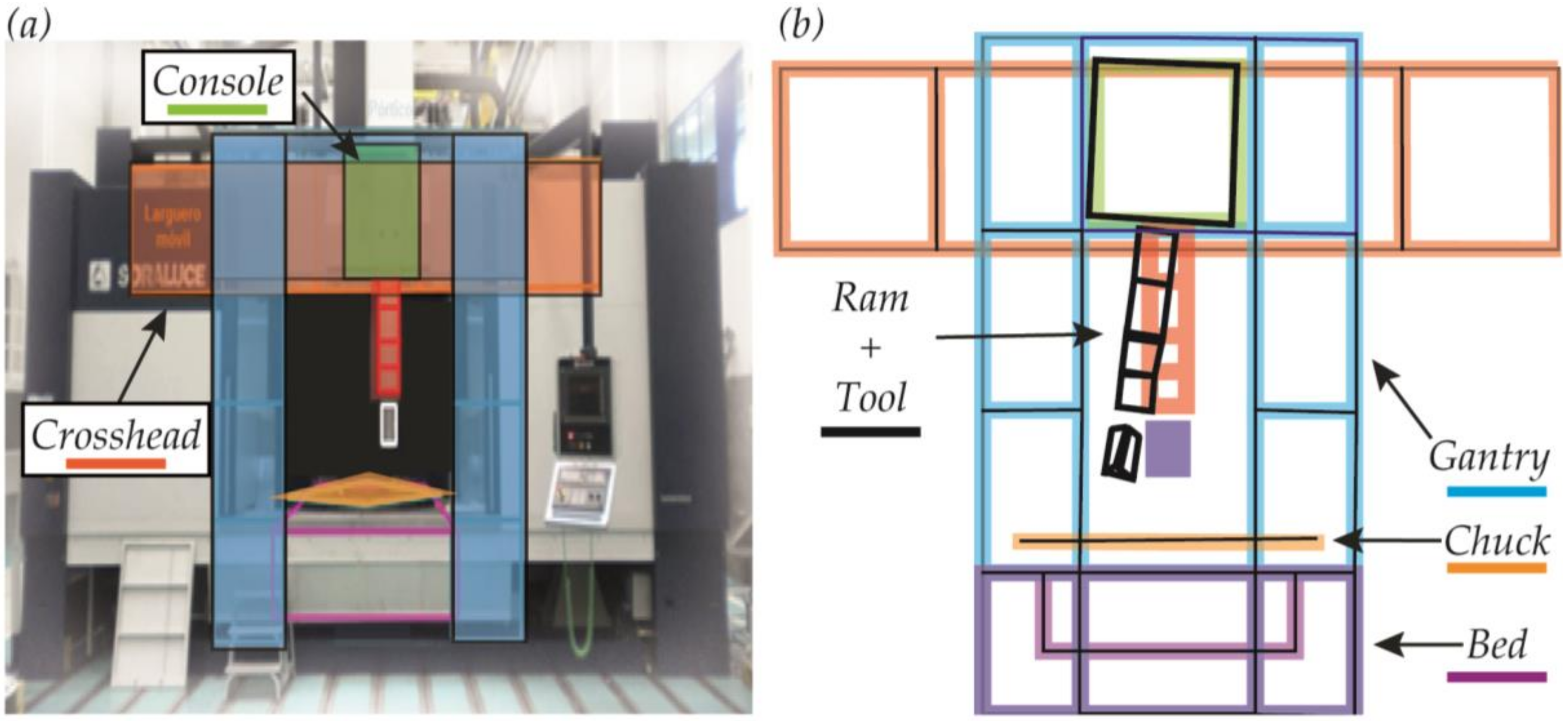
An experimental modal analysis has been carried out in order to analyse the dynamic behaviour of the machine. An instrumented impact hammer (PCB 086D20) is used to excite the structure at the ‘tool-tip’, and a triaxial accelerometer (PCB 356A16) is moved along several points of the machine structure to measure the acceleration response. Figure 4a shows the overall machine description with the ram being placed at its maximum overhang (1500 mm). Figure 4b shows the main modal shape of the machine ram, identified at 35 Hz, with a damping ratio of 2.6%.

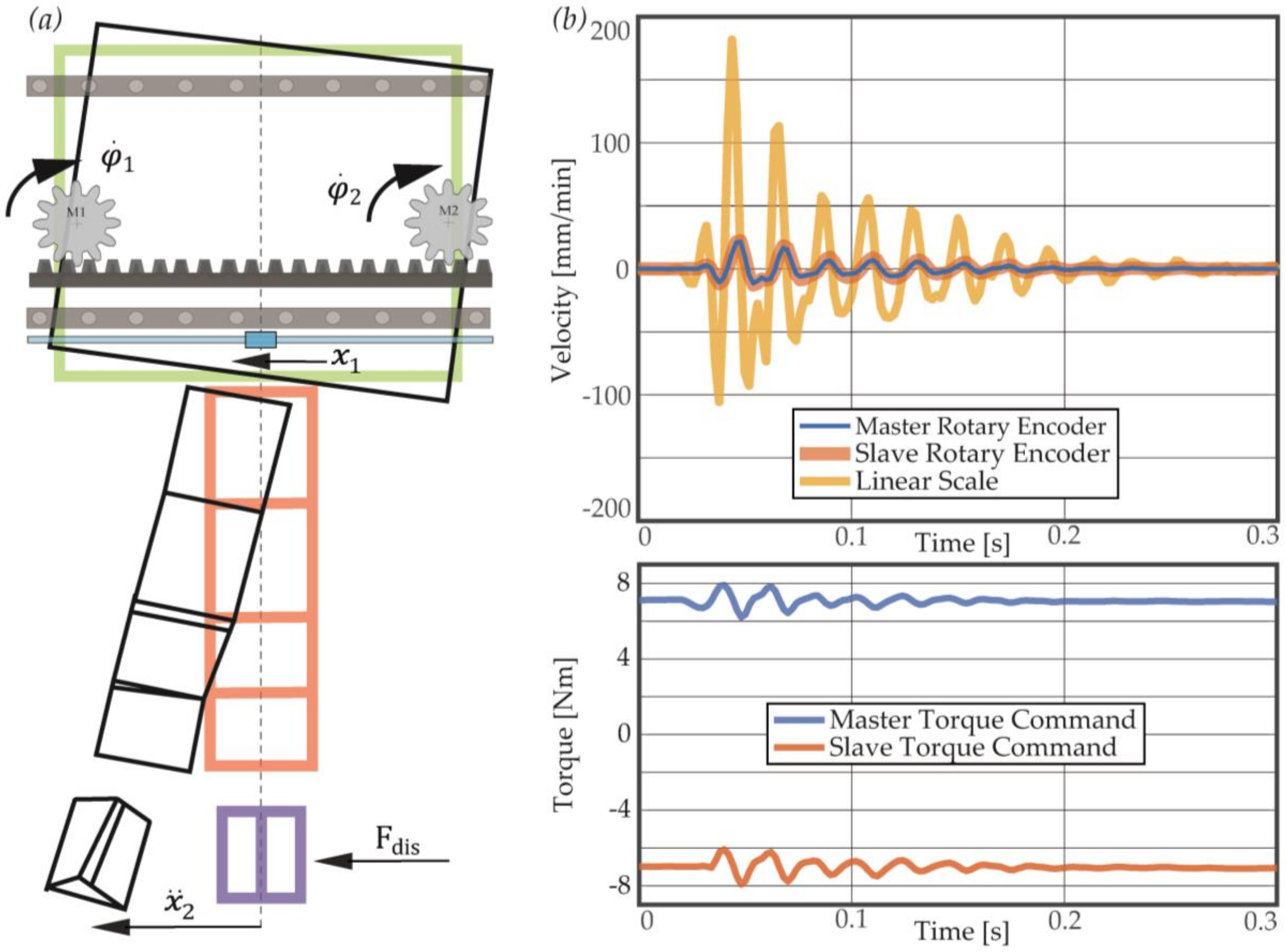
Figure 5a shows a detailed view of the ram and console with an overlaid sketch of the feed drive system used for x-axis positioning. The deformed shape of the machine is overlapped, where it can be seen that the mode is coming from the whole carriage rocking movement and the ram bending. This deformation due to a disturbance being applied at the tool centre point modifies the sensor readings. Figure 5b shows the CNC internal variable readings when an impact at the tool centre point is applied. As external perturbations are observable through the feedback encoders, the control actuation force will be directly affected, as shown in the commanded torque. This indicates that this particular mode shape is controllable and observable through the feed drive feedback system. Hence, the control parameters can affect the machine dynamic characteristics.

3.1. Commanded Preload Effect

Engelberth et al. [6] described how the bandwidth of the feed drive could be increased by raising the commanded preload value when the dynamics were limited by the servo system’s natural frequencies. This section studies the commanded preload effect at the tested machine tool dynamics.

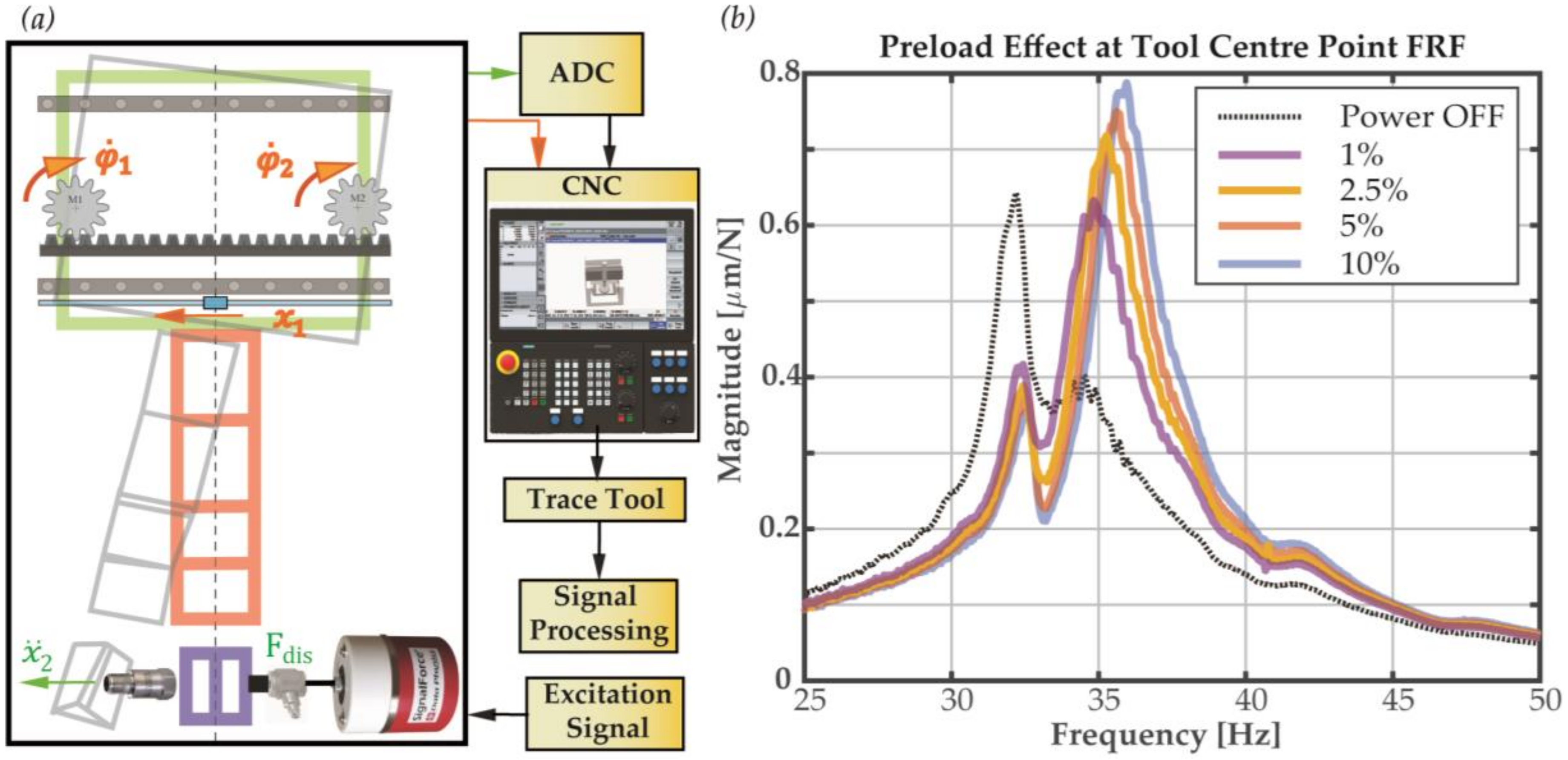
Figure 6a shows the experimental setup conceptual sketch, where the disturbance has been applied through a medium-size shaker that delivers up to 100N force (GW-V20/PA100E). The force used to dynamically excite the machine has been measured by means of a load cell (PCB 208C02) placed at the shaker’s stinger. At the same time, the ‘tool-tip’ acceleration has been measured by using an industrial accelerometer (PCB 603C01). The quality of the FRFs used to build the model is of vital importance, as the mathematical model derived in Section 2.2 is based on complex vector operations. For that reason, the use of the shaker rather than the dynamometric impact hammer has been considered. The machine tool is equipped with a SIEMENS 840D Solution Line CNC, which offers a data logger tool, called ServoTrace. In addition, a fast analogue to digital switch converter has been installed to be able to measure both ‘tool-tip’ acceleration and applied disturbance force. This implies that internal and external variables are synchronously acquired at the same sampling frequency of 500 Hz.

Figure 6b shows the influence of the commanded torque bias $\left(M_{\mathrm{T}}\right)$ on the dynamical response at the tool centre point. The shaker actuator is fed with a chirp signal from 25 Hz to 100 Hz, covering the frequency range of interest, in order to obtain the FRFs. The excitation is repeated four times to improve the response coherence, and the chirp length has been fixed to 20 s, as this yields an overall high quality measurement with sufficient frequency resolution. As expected, the preload value modifies the boundary conditions of the feed drive system, which directly affects the x-axis machine dynamic characteristics. A higher preload value shows an increment in the machine natural frequency, as well as a decrease of the damping ratio (see

Table 1. Modal parameters of the machine tool for different preload values.

Preload Value [%]	Natural Frequency [Hz]	Damping Ratio [%]	Modal Stiffness [N/µm]	Modal Mass [kg]
1	34.8	3.2	25.03	522
2.5	35.3	2.9	24.34	496
5	35.6	2.7	24.85	495
10	36	2.6	24.65	482

), especially for the main resonance at 35 Hz. In the same way, the remarkable difference between a non-powered (Power OFF) and powered frequency responses can be emphasized. The main mode shifts to a poorly damped 32 Hz resonance and the second main mode shape (35 Hz) almost disappears due to the high damping value.

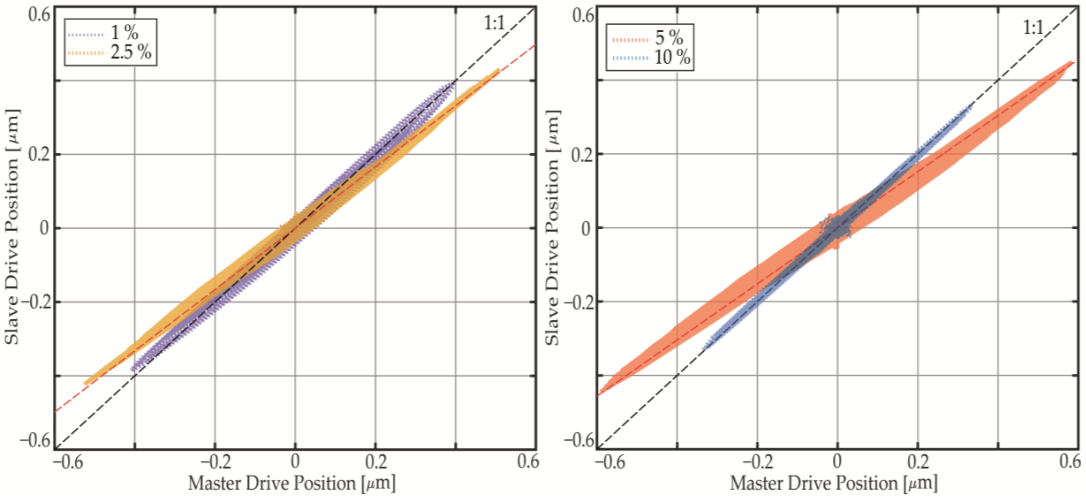
The user-defined preload magnitude should be high enough to suppress the existing backlash, as previously commented in Section 1. Figure 7 shows the master and slave rotary encoder-captured displacement in response to disturbance excitation that was applied at the tool centre point. As can be seen, the commanded preload value plays an important role in modifying the displacement ratio between the two motors. This ratio should ideally be 1:1 to have a balanced displacement of both motors. This ideal is closely achieved with a preload value of 10%, where the behaviour is similar to a straight line. In contrast, for 5% and 2.5% preload, it can be seen how the displacement ratio varies. Finally, the response for 1% also achieves an almost ideal ratio on average, but, when compared to the 10% response, the 1%, 2.5%, and 5% cases also show dynamic variation in the instantaneous displacement ratio, being marked by the increase in width for the phase plane plots between the master and slave drive positions.

3.2. Machine Open-Loop Extraction

The first step is to characterize both the controller and the open-loop response of the machine assembly in order to predict the effect of the control parameters on the dynamics of the machine.

The controller can be characterized by the schemes that the CNC manufacturers provide in their documentation. The dynamic characterization of the machine, however, involves difficulties, such as non-linearities due to friction or machine joints. In addition, the machine dynamics can significantly vary, depending on the cutting position, as shown in [15]. Similarly, the dynamic behaviour of the machine changes significantly with and without electrical power. Therefore, obtaining the response without the controller effect cannot be achieved by means of a non-powered frequency response. This would lead to non-linear behaviour, such as backlash, normally being suppressed by the preload provided by the controller, to become very significant. For this reason, a fixed preload value of 10% has been applied during the proceeding tests. However, the invariance of this control parameter would lead to developing certain assumptions that are described in Section 3.2.2.

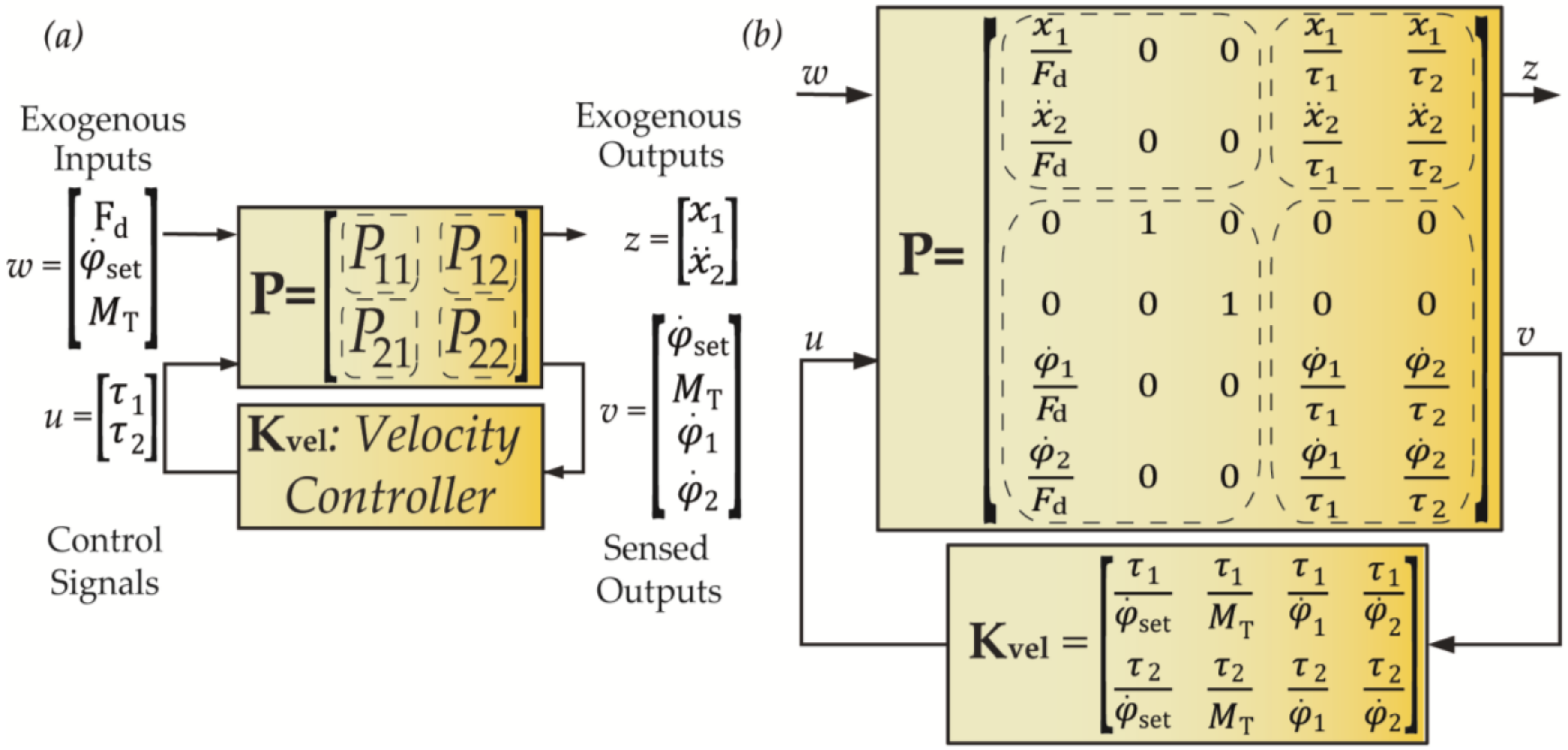
Furthermore, a dedicated ‘compiled cycle’ has been developed to allow for the addition of external commands to position, velocity, and torque reference points. This offers the possibility to inject a specified signal into the machine and excite it through the existing feed drive actuators. With this, and the ServoTrace tool mentioned earlier, the matrix P that defines the open-loop MIMO FRF for the machine, for a certain position, can be measured through excitation via the two kinds of input sources: the disturbance force Fdis and the motor torques (${\tau }_1$, ${\tau }_2$).

3.2.1. Tool Centre Point Force Disturbance Side Characterization

As previously discussed, the machine dynamical behaviour (Figure 6b) is different with and without electrical power, especially due to the variation of the preload. For that reason, in this research, the machine has been powered up, but the control parameters have been set to very low values (Kv = 1 [(m/min)/mm], Ti = 50 [ms], and Kp = 0.05 [Nms/rad]) to minimize the influence of the control actuation force while maintaining the preload of 10%. On the other hand, the experiment has been conducted four times, obtaining, as a result, an average response with a successful signal coherence check in order to increase the signal quality and minimize the uncertainty. 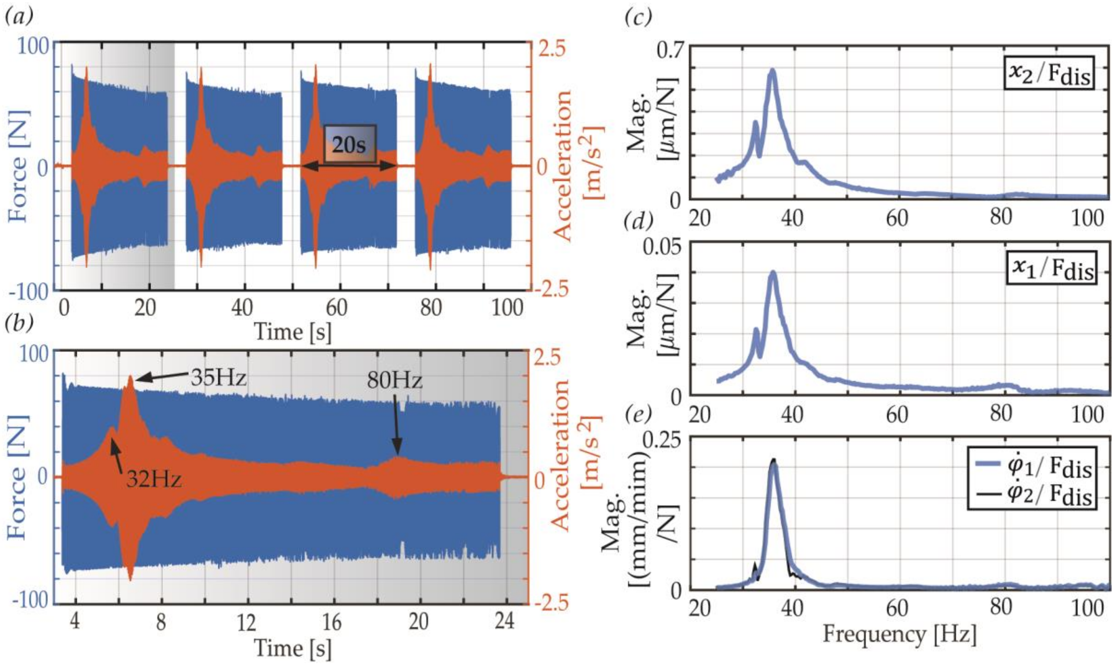Figure 8a shows the complete (four sections of 20 s) acquired time-domain data for the disturbance force and ‘tool-tip’ acceleration. The exerted force amplitude of the electromagnetic actuator located at the tool tip decay almost linearly with the excitation frequency. At the beginning of the excitation (25 Hz), the force amplitude is close to 70 N and, as a result, of the actuator’s response characteristics, at 100 Hz the force has decreased up to 60 N (Figure 8b). However, under the assumption of a linear system, this does not generate major problems. The time-domain acquired data show the dynamic behavior of the tested machine, where two clear amplifications are present at 5.8 s and 6.3 s. The two rotary and linear encoders’ data are synchronously registered in order to generate the FRFs that are shown in Figure 8c–e. The main two natural frequencies are located at 32 Hz and 35 Hz, as expected from the experimental analysis and time-domain data. Moreover, the frequency domain magnitude difference of roughly a factor ten between the cutting point (Figure 8c) and linear scale (Figure 8d) sensors can be explained by the mode shape that is shown in Figure 4.

The data represented in Figure 8c–e is used to fill the first column of the P matrix (Figure 2b).

3.2.2. Feed Drive Response Characterization

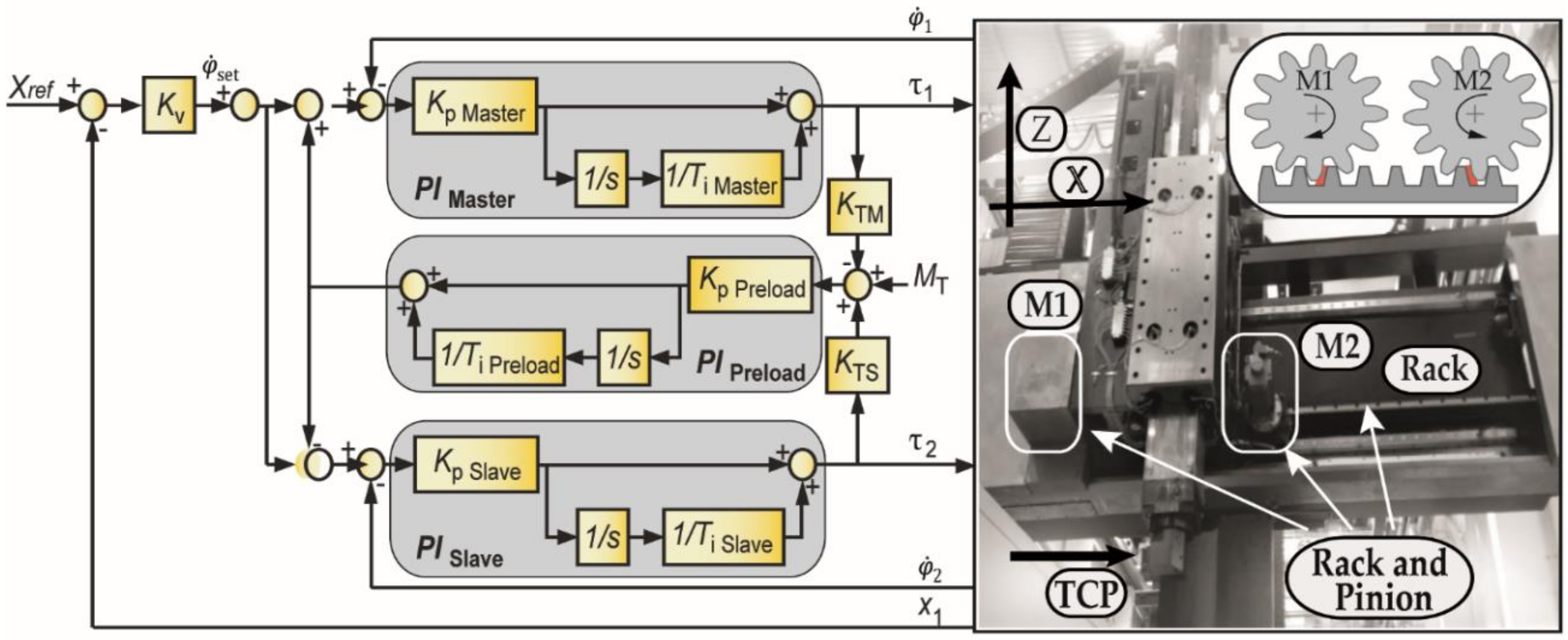
The response to excitation from both machine actuators is required to be able to couple the analytically defined controller effect and machine tool structural dynamics. Usually, the machine feed drive actuators should be individually excited in order to characterize the response. However, the tested machine uses a double pinion and rack mechanism with a Master–Slave control coupling, as described in Section 2.1. In achieving the removal of backlash, the ‘torque equalization controller’ couples both motor’s actuation. This means that, even if the excitation signal is carried out by a single motor, due to the torque equalization controller, the secondary motor also follows the excitation signal to obtain the desired torque bias. Hence, the response at a specific output point $O$ is affected by both motors’ excitation (${\tau }_1$, ${\tau }_2$). In the following equations the general output $O$ can be replaced by any output of the matrix P ($x_1$, ${\ddot{x}}_2$, ${\dot{\phi }}_1$ and ${\dot{\phi }}_2$).

$$O=\left(\frac{O}{{\tau }_1}\right)·{\tau }_1+\left(\frac{O}{{\tau }_2}\right)·{\tau }_2$$

(17)

The expressions in (18)–(19) can be used in order to be able to decouple the motor actuations and obtain the individual excitation response from each motor. The aim is to get at least two non-proportional measurements of the desired input (${\tau }_1$, ${\tau }_2$) and output ($O$). These measurements can be obtained by modifying the velocity PI controller of each motor independently. This will generate a different torque command for each motor. As shown, the resolution of the system FRF that is composed of two or more experimental measurements with different controllers allows for obtaining the open-loop frequency response functions of the matrix P.

$$\underset{X}{\underbrace{{\left[\begin{array}{cc}\underset{K_1}{\underbrace{O}}& \underset{K_2}{\underbrace{O}}\end{array}\right]}_{1x2} }}=\underset{G}{\underbrace{{\left[\underset{\forall K}{\underbrace{\begin{array}{cc}\left(\frac{O}{ {\tau }_1}\right)& \left(\frac{O}{{\tau }_{2 }}\right)\end{array}}} \right]}_{1x2 }}}·\underset{U}{\underbrace{{\left[\begin{array}{cc}{\tau }_1& {\tau }_1\\ \underset{K_1}{\underbrace{{\tau }_{2 }}}& \underset{K_2}{\underbrace{{\tau }_{2 }}}\end{array}\right]}_{2x2 }}}$$

(18)

$$X=G·U \to G=X·inv \left(U\right)$$

(19)

Even though the procedure described above is valid for a general case, for the research reported in this paper, this method could not be implemented due to practical reasons that are associated with the control system measurement. However, the following simplifications have been considered due to the machine topology. Both motors are identical, they have the same weighting factors ${(K}_{\mathrm{TM}}=K_{\mathrm{TS}}=0.5)$ and PI gains ($P{I}_{\mathit{Master}}=P{I}_{\mathit{Slave}})$, so it is assumed that the same torque command is generated for both motors $\left({\tau }_1={\tau }_2\right)$. In addition to this, if the excitation signal is given as a velocity command through a compiled cycle in the CNC, the generated reference torque $\left({\tau }_0\right)$ will be equally divided between both motors $\left({\tau }_1={\tau }_2={\tau }_0/2\right)$. This assumption is only valid when the static part of the torque command is removed, for example, for the selected excitation frequency band (25 to 100 Hz).

$$O=\left(\frac{O}{{\tau }_1}\right)·{\tau }_1+\left(\frac{O}{{\tau }_2}\right)·{\tau }_2=\left(\frac{O}{{\tau }_1}\right)·\frac{{\tau }_0}{2}+\left(\frac{O}{{\tau }_2}\right) ·\frac{{\tau }_0}{2}=\left(\left(\frac{O}{{\tau }_1}\right)+\left(\frac{O}{{\tau }_2}\right) \right)·\frac{{\tau }_0}{2}$$

(20)

In addition, when considering that the motors and sensors are symmetrically located with respect to the machine’s main resonance mode shape, the frequency response can be equalized $\left(O/{\tau }_1\right)=\left(O/{\tau }_2\right)$. This assumption can be extrapolated to all of the measured outputs referred to in this paper ($x_1$, ${\ddot{x}}_2$, ${\dot{ \phi }}_1$, and ${\dot{\phi }}_2$).

$$O=\left(\left(\frac{O}{{\tau }_1}\right)+\left(\frac{O}{{\tau }_2}\right)\right)·\frac{{\tau }_0}{2}=\sout{2}·\left(\frac{O}{{\tau }_1}\right)·\frac{{\tau }_0}{\sout{2}}=\left(\frac{O}{{\tau }_1}\right)·{\tau }_0$$

(21)

With the previous hypotheses, it is assumed that the open-loop frequency response functions can be obtained, even if both of the motors are simultaneously exciting the system. With the tested tension torque of 10%, the time-domain amplitude difference between the torque commands (${\tau }_1$, ${\tau }_2$) is ±0.5 Nm, or an 88% of equivalence. At the same time, the frequency response function between both torque commands have shown a +0% and −15% amplitude difference with respect to the ideal ratio of 1:1 within the frequency range of interest. These assumptions demonstrate the capabilities and limitations of the developed simulation model, as the velocity PI controller gains for each motor cannot be independently modified. Additionally, the followed measurement methodology cannot be generalized to all machine configurations, for example, to machines having different motors and different weighting factors for the preload. Nonetheless, in the case of the studied machine tool, the practically obtained FRFs via dual motor excitation can still be used. Future research will address these points and investigate the decoupling of individual single-input FRFs from experimental multi-input frequency response data.

Similar to the previous subsection, Figure 9a,b shows the acquired time-domain signals. As the excitation signal has been placed outside the velocity feedback loop, it can be seen in Figure 9a how the torque commands are sensitive to the structural vibrations. In addition to this, as a result of the Master–Slave coupling configuration, both commanded torques are of inverse sign to successfully suppress the existing backlash. The static value is ±7 Nm as the preload value is set to 10% of the motor rated torque (70 Nm). The excitation chirp signal is added to this static value. Figure 9b shows the acquired data for both rotary encoders and cutting point acceleration during the excitation process. The machine tool structural resonance at 35 Hz generates an anti-resonance at the same frequency in both rotary encoders, as seen in Figure 9c. Moreover, this is how the machine tool natural frequency interacts with the specified servo controller. This resonance manifests itself as an anti-resonance in the encoder feedback. Furthermore, when commissioning the velocity loop, the implemented control parameters affect the characteristics of the resonance on the machine ‘tool-tip’ side, and its reflection back to the control loop as anti-resonance.

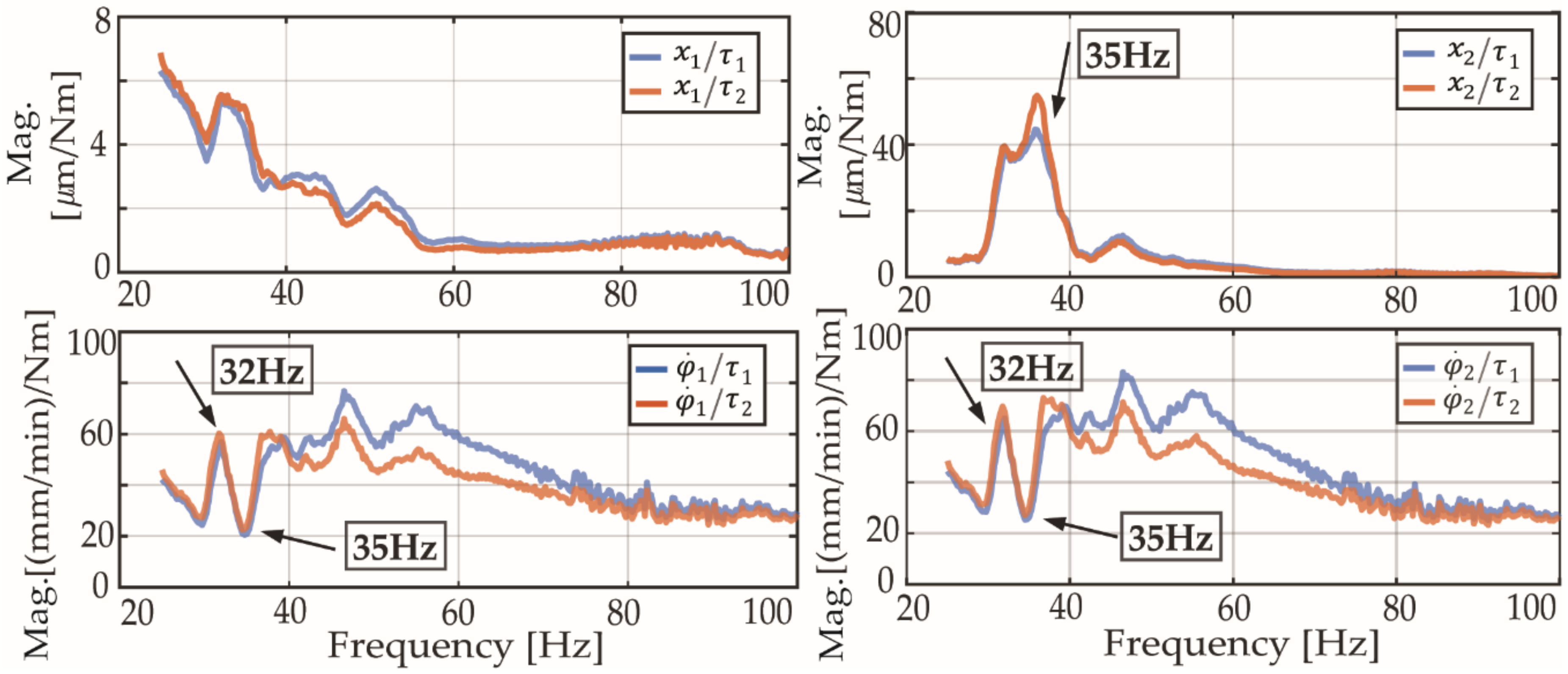
Figure 10 shows the computed frequency responses from both actuators to the linear scale, ‘tool-tip’ displacement, and both rotary encoders ($x_1$, $x_2$, ${\dot{\phi }}_1$, and ${\dot{\phi }}_2$). Those frequency response functions are directly obtained from the experiment realized with both motors acting simultaneously on the system. These ‘pseudo’ open-loop responses are used in the matrix P under the hypotheses that the motors and the velocity controllers are identical. The figure validates the hypotheses, as the responses are practically similar up to 40 Hz. Furthermore, the complexity of the responses shows the advantage of deriving the model in the frequency-domain rather than performing the curve fittings needed for time-domain analyses. Analysing the frequency response magnitudes in detail, the previously commented order of magnitude difference between the linear scale and ‘tool-tip’ accelerometer is present. Additionally, the commented resonance at 35 Hz in the accelerometer generates an anti-resonance (or motor-locked frequency) in both rotary encoders.

The frequency-domain signals that are shown in Figure 10 are used in the P matrix as ‘pseudo’-open-loop responses. With the experimental characterization presented in this section, the analytical effect of the implemented controller can be coupled with the machine tool dynamics.

4. Closed-Loop Response Simulations

This section shows the prediction and experimental tool centre point closed-loop responses for velocity proportional (Kp), integral time (Ti), and position proportional (Kv) gain variations. In the subsequent comparisons, the value of the studied control parameter has been modified, defining as invariant the other two remaining parameters. Note, the commanded preload value is fixed at 10%, as previously commented. In addition, the same parameterization has been defined for both servomotor velocity controllers ($P{I}_{\mathrm{Master}}$ = $P{I}_{\mathrm{Slave}}$).

4.1. Velocity Proportional Gain Kp

Zirn [7] and Uriarte et al. [4] pointed out the importance of the proportional velocity gain in the context of the damping amount that the feed drive system might be able to influence around a particular resonance. The effect is mainly because this gain alters the mechanical pole location; thus, this alters both the natural frequency and damping ratio. Figure 11 shows the comparison of the machine tool closed-loop FRF at the tool centre point for different values of the tested control parameter value. In this example, the remaining feedback gains are tuned to conservative values that would typically be found in a production environment (Kv = 1 [(m/min)/mm] and Ti = 10 [ms]). The model can predict the tendency to increase the ‘tool-tip’ compliance when the proportional velocity gains are increased. In addition, the resonance of 32 Hz is not significantly modified with the variation of this gain.

The modal parameters for the 35 Hz mode have been extracted in order to see the effect of the velocity proportional gain on the machine tool compliance.

Table 2. Modal parameters of the machine tool for different velocity proportional gain values.

Kp [Nms/rad]	Natural Frequency [Hz]	Damping Ratio [%]	Modal Stiffness [N/µm]	Modal Mass [kg]
0.5	35.71	3.2	24.31	483
1	35.71	3	24.75	492
2.5	35.66	2.7	24.42	486
5	35.95	2.6	24.43	479

shows how the natural frequency is slightly modified, but the damping ratio can be modified up to 20% for this machine.

4.2. Velocity Integral Time Gain Ti and Position Proportional Gain Kv

Figure 12 shows the velocity integral time effect at the ‘tool-tip’. This gain does not modify the machine tool dynamic behaviour much, as can be seen in both experimental and predicted frequency responses. For this test, the proportional velocity and position gains were respectively fixed to 2.5 [Nms/rad] and 1 [(m/min)/mm]. Figure 13 shows the position proportional gain effect. As in the previous case, the position loop gain does not change the tool tip dynamic response much, at least for the tested machine tool.

These conducted tests validate the frequency domain-based MIMO model and the hypotheses carried out in Section 3.2.2, as it captures the experimentally observed tool centre point dynamic behaviour for different control parameter variations.

5. Conclusions

In large machine tool applications, with low machine natural frequencies and mode shapes that affect the feedback sensor measurements, the parametrization of the feed drive controller could affect the dynamical response at the machine tool centre point. The double pinion and rack feed drive system is usually implemented in large machine tools requiring long travel strokes. The commanded preload value plays an important role in reducing the backlash between the gears and rack, as well as in modifying the machine tool dynamics. The most relevant conclusions obtained from the conducted research are summarized, as follows:

• The experimental observations show the influence of the machine tool dynamics at the servo feedback sensor reading. The response amplitude is determined by the dynamic characteristics of the machine (experimentally obtained by experimental modal analysis) and the location of the feedback sensors.
• Machine tool structural flexibilities (i.e., the main resonance at 35 Hz) correspond to anti-resonances (motor-locked frequency) in positioning sensor reading. This fact shows how the machine tool structural dynamics and servo controller interact and, hence, modify the cutting point compliance.
• Master–Slave commanded coupling force can modify the machine tool dynamics at the cutting point. The natural frequency of the main flexibility is slightly altered (from 35 Hz to 36 Hz), and the damping ratio varies from 3.2% to 2.6% as a result of the variation of the electronic preload.
• A MIMO model for coupling the servo controller effect and machine tool structural dynamics has been developed. The machine tool dynamic behaviour has been characterized from external disturbances by means of a shaker and the machine’s own actuators, through a dedicated compiled cycle implemented in the industrial CNC.
• The frequency-domain based MIMO model has been successfully validated by comparing the predicted machine closed-loop frequency responses to the experimental ones.
• The proportional velocity loop gain is the most critical parameter that influences the tool centre point compliance. The integral time gain and the proportional position loop gain have a minor influence.

Following the line of the work discussed in this research, the following steps can be targeted:

• The derived MIMO model could use the Finite Element simulation results to obtain the open-loop dynamic matrix responses and help during the machine design phase.
• Even though lower velocity proportional gains are desirable for improving the machine tool damping characteristics, a deeper analysis using complementary techniques, such as root locus, can provide a better understanding of the effect of the control parameters.
• Experimental chatter stability cutting tests should also be realized to show the effect of the servo control loop on the machine tool cutting capabilities.

References

1. Altintas, Y.; Verl, A.; Brecher, C.; Uriarte, L.; Pritschow, G. Machine tool feed drives. CIRP Ann. 2011, 60, 779–796. [Google Scholar] [CrossRef]
2. Pritschow, G. A comparison of linear and conventional electromechanical drives. CIRP Ann. 1998, 47, 541–548. [Google Scholar] [CrossRef]
3. López De Lacalle, L.N.; Lamikiz, A. Machine Tools for High Performance Machining; Springer Science & Business Media: Berlin, Germany, 2008. [Google Scholar]
4. Uriarte, L.; Zatarain, M.; Axinte, D.; Yagüe-Fabra, J.; Ihlenfeldt, S.; Eguia, J.; Olarra, A. Machine tools for large parts. CIRP Ann. 2013, 62, 731–750. [Google Scholar] [CrossRef]
5. REDEX Racks and Pinions. Available online: www.redex-andantex.com (accessed on 23 October 2019).
6. Engelberth, T.; Apprich, S.; Friedrich, J.; Coupek, D.; Lechler, A. Properties of electrically preloaded rack-and-pinion drives. Prod. Eng. 2015, 9, 269–276. [Google Scholar] [CrossRef]
7. Zirn, O. Machine Tool Analysis-Modelling, Simulation and Control of Machine Tool Manipulators, A Habilitation Thesis; ETH Zurich: Zurich, Switzerland, 2008. [Google Scholar]
8. Heidenhain. Technical Manual TNC640; Heidenhain: Traunreut, Germany, 2015. [Google Scholar]
9. Verl, A.; Engelberth, T. Adaptative preloading for rack-and-pinion drive systems. CIRP Ann. 2018, 67, 369–372. [Google Scholar] [CrossRef]
10. Pritschow, G. On the influence of the velocity gain factor on the path deviation. CIRP Ann. 1996, 45, 367–371. [Google Scholar] [CrossRef]
11. Erkorkmaz, K.; Kamalzadeh, A. High bandwidth control of ball screw drives. CIRP Ann. 2006, 55, 393–398. [Google Scholar] [CrossRef]
12. Bearee, R.; Barre, P.J.; Bloch, S. Influence of high-speed machine tool control parameters on the contouring accuracy. Application to linear and circular interpolation. J. Intell. Robot. Syst. 2004, 40, 321–342. [Google Scholar] [CrossRef]
13. Lee, K.; Ibaraki, S.; Matsubara, A.; Kakino, Y.; Suzuki, Y.; Arai, S.; Braasch, J. A servo parameter tuning method for high-speed NC machine tools based on contouring error measurement. WIT Trans. Eng. Sci. 2003, 44. [Google Scholar] [CrossRef]
14. Feng, B.; Zhang, D.; Yang, J.; Ren, G. Control parameters auto-tuning for bi-axial servo feed system. Procedia CIRP 2014, 17, 841–846. [Google Scholar] [CrossRef] [Green Version]
15. Iglesias, A.; Munoa, J.; Ciurana, J. Optimisation of face milling operations with structural chatter using a stability model based process planning methodology. Int. J. Adv. Manuf. Technol. 2014, 70, 559–571. [Google Scholar] [CrossRef]
16. Munoa, J.; Beudaert, X.; Dombovari, Z.; Altintas, Y.; Budak, E.; Brecher, C.; Stepan, G. Chatter suppression techniques in metal cutting. CIRP Ann. 2016, 65, 785–808. [Google Scholar] [CrossRef]
17. Munoa, J.; Beudaert, X.; Erkorkmaz, K.; Iglesias, A.; Barrios, A.; Zatarain, M. Active suppression of structural chatter vibrations using machine drives and accelerometers. CIRP Ann. 2015, 64, 385–388. [Google Scholar] [CrossRef]
18. Beudaert, X.; Barrios, A.; Erkorkmaz, K.; Munoa, J. Limiting factors for the active suppression of structural chatter vibrations using machine’s drives. In Proceedings of the XIIth International Conference on High Speed Machining (HSM 2015), Nanjing, China, 18–20 October 2015; Available online: https://hal.archives-ouvertes.fr/hal-01342267 (accessed on 3 October 2019).
19. Mohammadi, Y.; Ahmadi, K. Frequency domain analysis of regenerative chatter in machine tools with linear time periodic dynamics. Mech. Syst. Signal Process. 2019, 120, 378–391. [Google Scholar] [CrossRef]
20. Iglesias, A.; Dombovari, Z.; Gonzalez, G.; Munoa, J.; Stepan, G. Optimum selection of variable pitch for chatter suppression in face milling operations. Materials 2019, 12, 112. [Google Scholar] [CrossRef] [Green Version]
21. Herranz, G.; Antolínez, A.; Escartín, J.; Arregi, A.; Gerrikagoitia, J.K. Machine tools anomaly detection through nearly real-time data analysis. J. Manuf. Mater. Process. 2019, 3, 97. [Google Scholar] [CrossRef] [Green Version]
22. Merino, R.; Bediaga, I.; Iglesias, A.; Munoa, J. Hybrid edge-cloud based smart system for chatter suppression in train wheel repair. Appl. Sci. 2019, 9, 4283. [Google Scholar] [CrossRef] [Green Version]
23. Altintas, Y.; Brecher, C.; Weck, M.; Witt, S. Virtual Machine Tool. CIRP Ann. 2005, 54, 115–138. [Google Scholar] [CrossRef]
24. Albertelli, P.; Cau, N.; Bianchi, G.; Monno, M. The effects of dynamic interaction between machine tool subsystems on cutting process stability. Int. J. Adv. Manuf. Technol. 2012, 58, 923–932. [Google Scholar] [CrossRef]
25. Beudaert, X.; Mancisidor, I.; Miguel, L.; Barrios, A.; Erkorkmaz, K.; Munoa, J. Analysis of the feed drives control parameters on structural chatter vibrations. In Proceedings of the XIIIth International Conference on High Speed Machining (HSM 2016), LEM3, Metz, France, 4–5 October 2016. [Google Scholar]
26. Grau, J.; Sulitka, M. Influence of Linear Feed Drive Controller Setting in CNC Turning Lathe on the Stability of Machining. J. Mach. Eng. 2019, 19, 182–184. [Google Scholar] [CrossRef]
27. Zaeh, M.; Rebelein, C.; Semm, T. Predictive simulation of damping effects in machine tools. CIRP Ann. 2019, 68, 393–396. [Google Scholar] [CrossRef]
28. Gross, H.; Stute, G. Elektrische Vorschubantriebe für Werkzeugmaschinen; SIEMENS: Munich, Germany, 1981. [Google Scholar]
29. Koren, Y.; Lo, C.C. Advanced Controllers for Feed Drives. CIRP Ann. 1992, 41, 689–698. [Google Scholar] [CrossRef]
30. Skogestad, S.; Postlethwaite, I. Multivariable Feedback Control: Analysis and Design, 2nd ed.; Wiley: Hoboken, NJ, USA, 2005. [Google Scholar]
Figure 1. General Master-Slave configuration control structure and analysed machine servo details.
Jmmp 04 00033 g001
Figure 2. (a) Velocity controller Linear Fractional Transformation (LFT) definition, (b) Matrix frequency domain relationship detail.
Jmmp 04 00033 g002
Figure 3. (a) Position controller LFT definition, (b) Matrix frequency domain relationship detail.
Jmmp 04 00033 g003
Figure 4. (a) Machine modal analysis description, (b) Ram mode displacement.
Jmmp 04 00033 g004
Figure 5. (a) Modal shape deformation detail, (b) Velocity and Torque CNC internal variables reaction to Fdis.
Jmmp 04 00033 g005
Figure 6. (a) Overall experimental implementation concept sketch, (b) Tool centre point frequency response function (FRF) for different preload values.
Jmmp 04 00033 g006
Figure 7. Master and slave displacement ratios due to a disturbance force.
Jmmp 04 00033 g007
Figure 8. (a,b) Time-domain force and acceleration signals, (ce) Computed FRFs.
Jmmp 04 00033 g008
Figure 9. Time-domain signals for (a) torque commands, (b,c) rotary encoders and acceleration signals.
Jmmp 04 00033 g009
Figure 10. Computed FRFs from machine side actuation.
Jmmp 04 00033 g010
Figure 11. (a) Experimental; (b) Predicted closed-loop tool centre point dynamics.
Jmmp 04 00033 g011
Figure 12. (a) Experimental, (b) Predicted closed-loop tool centre point dynamics.
Jmmp 04 00033 g012
Figure 13. (a) Experimental, (b) Predicted closed-loop tool centre point dynamics.
Jmmp 04 00033 g013