Review

Precision Permittivity Measurement for Low-Loss Thin Planar Materials Using Large Coaxial Probe from 1 to 400 MHz

School of Electrical Engineering, Faculty of Engineering, Universiti Teknologi Malaysia, 81310 Skudai, Johor, Malaysia
*
Author to whom correspondence should be addressed.
J. Manuf. Mater. Process. 2018, 2(4), 81; https://doi.org/10.3390/jmmp2040081
Submission received: 12 October 2018 / Revised: 23 November 2018 / Accepted: 27 November 2018 / Published: 3 December 2018

Abstract

:
This paper focuses on the non-destructive dielectric measurement for low-loss planar materials with a thickness of less than 3 mm using a large coaxial probe with an outer diameter of 48 mm. The aperture probe calibration procedure required only to make a measurement of the half-space air and three offset shorts. The reflection coefficient for the thin material is measured using a Keysight E5071C network analyzer from 0.3 MHz to 650 MHz and then converted to a relative dielectric constant, εr and tangent loss, tan δ via closed form capacitance model and lift-off calibration process. Average measurement error of dielectric constant, Δεr is less than 6% from 1 MHz to 400 MHz and the resolution of loss tangent, tan δ measurement is capable of achieving 10−3.

1. Introduction

Sensitivity, sustainability, and simplicity in operations are important requirements for sensing devices in large-scale material processing industries. To reduce the uncertainty of the measurements, the sensors should have a large sensing area, a high concentration of sensing field, and high sensitivity to the slight changes in material under test (MUT). The operating frequency of the permittivity, εr measurements in most of the material processing industries are up to a few hundred MHz [1,2,3].
The open-ended coaxial probe technique is a simple, broadband, and non-destructive way to measure the relative permittivity, εr of a material. Coaxial probes have been commercialized and used commonly since 1990 [4]. Recently, several probes have produced by manufacturers such as SPEAG Inc. [5], KEYCOM [6], and APREL Inc. [7]. However, coaxial probes (N-type’s or SMA’s diameter size) are less sensitive to small changes in the MUT especially for thin and low-loss materials in permittivity, εr measurement at MHz frequency. This causes the measurement results for low-loss materials at low frequencies to be highly scattered and less precise [8]. In fact, most coaxial probes are only suitable for half-space infinite lossy material with εr′ > 5 and tan δ > 0.05 [4,5,6,7,8,9,10,11].
In this study, a large open-ended coaxial probe was designed to overcome those issues, which is capable of measuring the εr of low-loss materials having thickness of 1 mm precisely from 1 to 400 MHz. The designed large probe is heavy whereby it is capable of supplying stable reflection measurements. Additionally, it is sensitive to measurements at low frequencies due to its large size. Furthermore, large probe aperture (sensing area) can reduce the uncertainty of measurement, which mostly caused by the inequality of composite distribution in MUT, especially for inhomogeneous MUTs. The probe design of the probe and its performance were analyzed in detail. An explicit formulation for the prediction of εr, which does not involve numerical inversion routines (iterative method) as in Refs. [8,9,10,11] is used. Since this study is focused on low frequencies measurement (up to 400 MHz), thus, a simple closed-form capacitance model [12,13,14,15,16,17,18] is implemented to predict the dielectric properties of MUT based on the measured reflection coefficient at probe aperture. The differences in this study compared with previous works are summarized in Table 1. In Refs. [8,9,10,11], the iterative methods (inverse methods) used to estimate the permittivity, εr of lossy MUT in which the predicted values of εr are obtained by minimizing the difference between the measured aperture reflection coefficient and the theoretical calculations. Those iterative methods are complicated solutions and less suitable for real-time εr estimation.
Although the probe designs in Refs. [8,9] did not use the transitions section on the boundary between the connector and the coaxial line, the mismatch reflection errors that exist on the boundary can be eliminated after the rigorous aperture calibration is performed. In fact, a high sensitivity measurement can be achieved by a method in which the MUT is filled in a coaxial line as in Refs. [11,12]. However, this measurement method encounters difficulties in the sample preparation stage in which the sample (MUT) must be identified to fully fill in without any air gap between the inner conductor and the outer conductor. Furthermore, it is only suitable for semi-liquid or powder form MUTs.

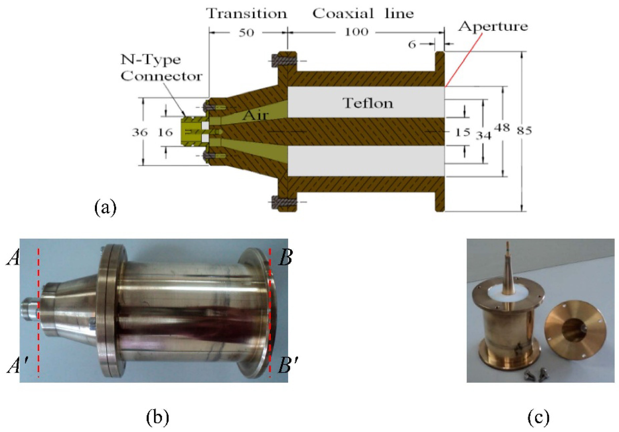
2. Large Coaxial Probe Design

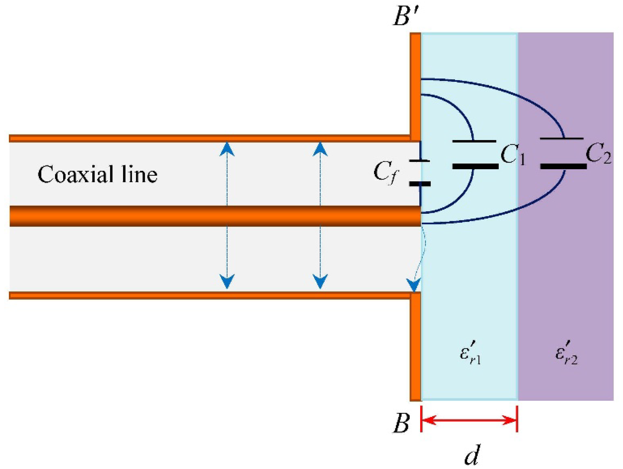
2.1. Coaxial Probe Formulations

The earliest coaxial probe formula derivation (during early 1950) [19] concerned the homogeneous case, which an air-filled coaxial line with an infinite conducting flange is radiated into the free space. The aperture normalized admittance, Y ˜ of the probe was expressed in variational integral equations. During that time, the main implementation of open-ended coaxial line is used as an antenna. The open-ended coaxial probe began to be applied as a dielectric probe sensor during early 1980s. The rigorous integral formulation was investigated back by Refs. [20,21]. However, those integrations are difficult to use to solve the inverse problem analytically. Thus, a lot of literature [13,14,15,16,17] formulated the aperture admittance in closed-form capacitance, Co terms in which it is easily used to estimate the relative complex permittivity, εr of MUT at low operating frequencies as follows:
Y ˜ = j ω ( ε r C o + C f ) / Y o
where Yo is the characteristic admittance of coaxial line. In 1986, the modeling of open-ended coaxial probe that is terminated by layered media was studied by Ref. [22]. Subsequently, probe modeling studies which considered multi-layer MUT were rapidly developed during 1990 [23,24,25,26,27,28,29,30,31,32,33].

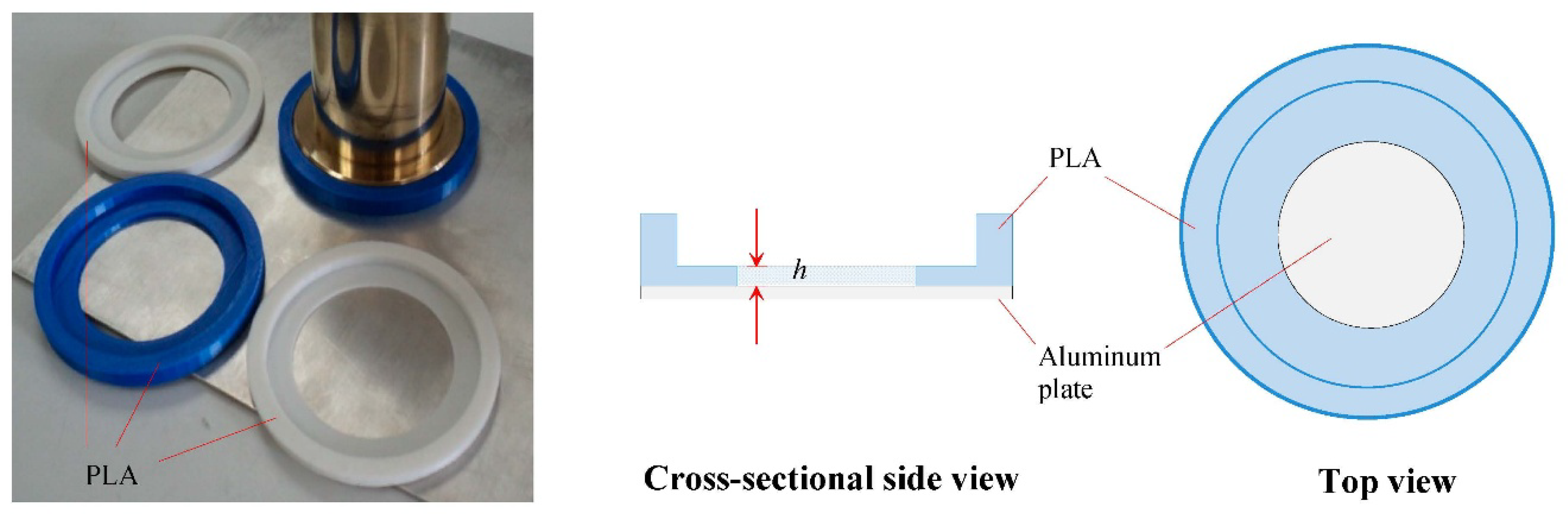
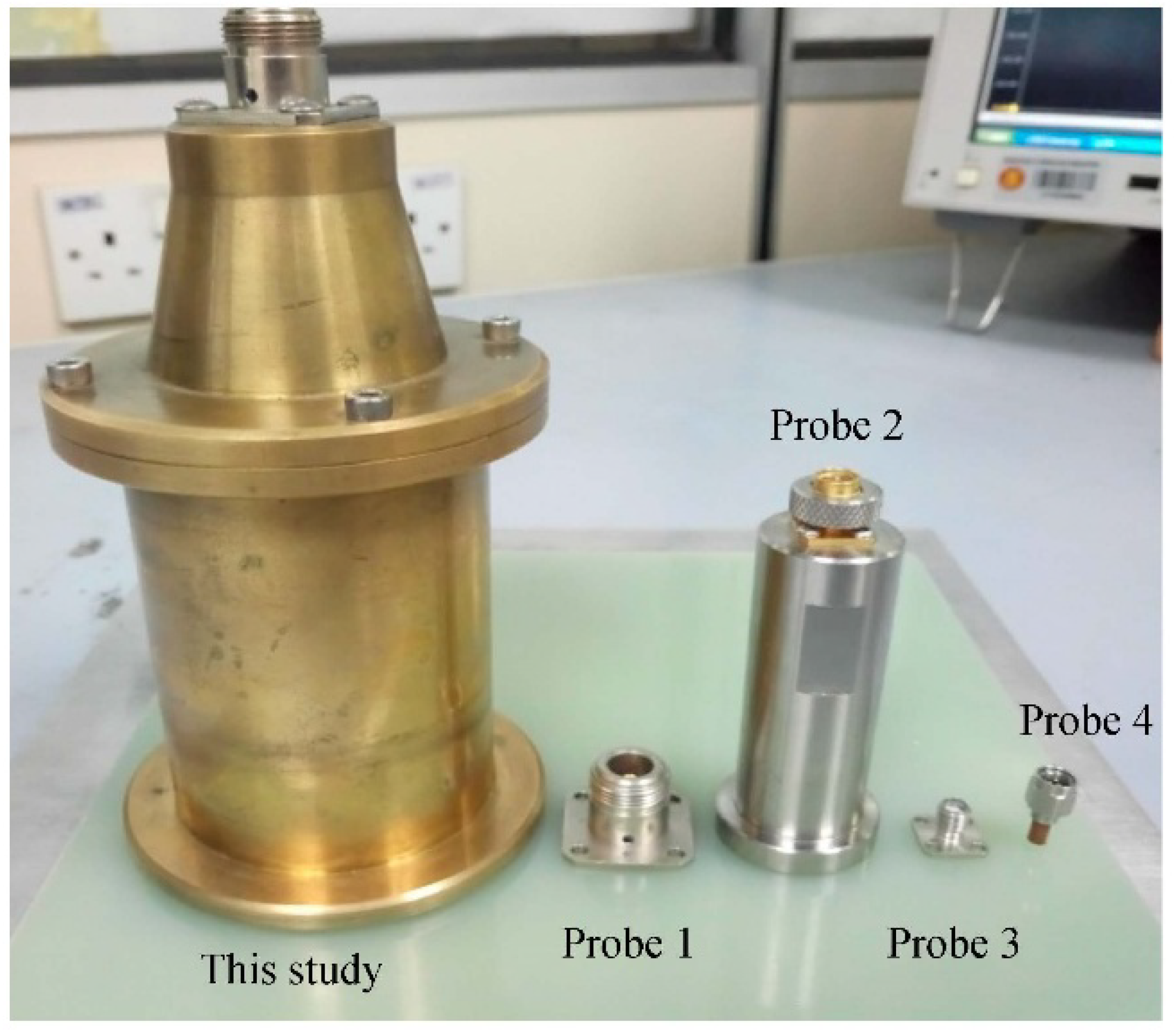
2.2. Dimensions and Structure

The designed coaxial probe as shown in Figure 1a is made of brass, since the material is relatively low cost and has slower surface oxidation process when it is exposed to the moisture in the air. The dimensions of the coaxial probe with outer radius of inner conductor, a = 7.5 mm and inner radius of outer conductor, b = 24.0 mm, were designed based on the characteristic impedance, Zo = [60 × ln(b/a)/√εc] = 50 Ω. The maximum limit of the operating frequency, fmax propagating in the coaxial line of the probe is determined using TE11 cut-off as: fmax = (3 × 10⁸)/[π(b + a)√εc] ≈ 2.1 GHz. In fact, the limit of operation frequency of the practice coaxial line is always much lower than the TE11 cutoff frequency based on the quality and precision of machining. The symbol εc (Air: εc = 1, Teflon: εc = 2.06) represents the relative permittivity of material filling in the coaxial line in between the inner and outer conductor. The total weight of the coaxial probe is 2.6 kg. It has been divided into three sections: (I) N-type connector, which is used to connect the coaxial probe with the network analyzer via cable. (II) Transition section, which is a 50 mm of air-filled conical taper. The radius a and b of the conductors are increased along the transition length with a constant ratio, b/a = 2.3. Ratio, b/a = 2.3 is required to maintain Zo = 50 Ω along the transition length to achieve low return loss and the lowest standing wave ratio (SWR) during the transformation from small to large coaxial line. (III) Large coaxial line section, which is a 100 mm length of 50 Ω Teflon-filled coaxial line with b/a = 3.3. The Teflon isolation block is used to prevent the MUT from getting into the coaxial line. In addition, Teflon has high flexural strength, excellent chemical resistance, and high stability over a wide temperature range.

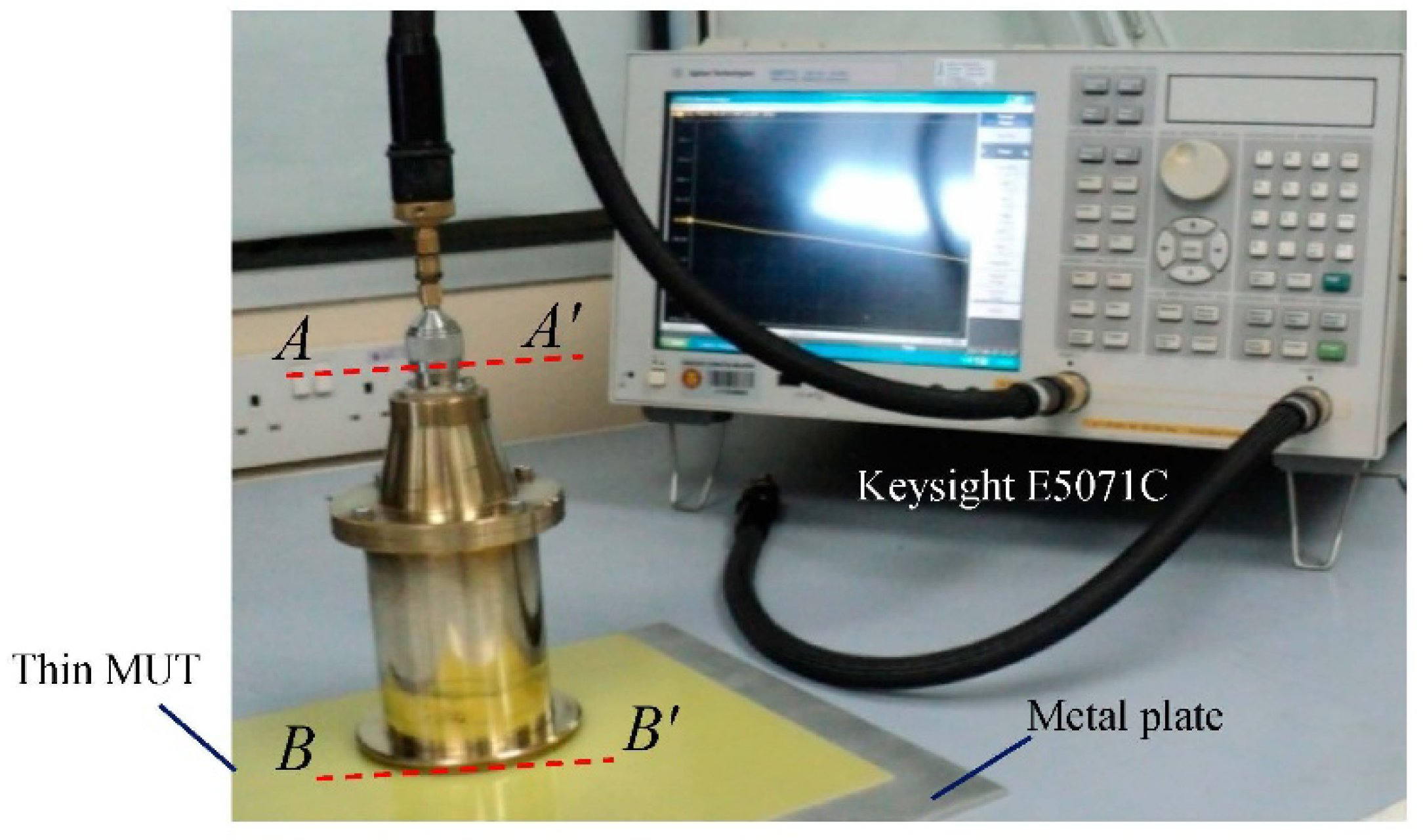
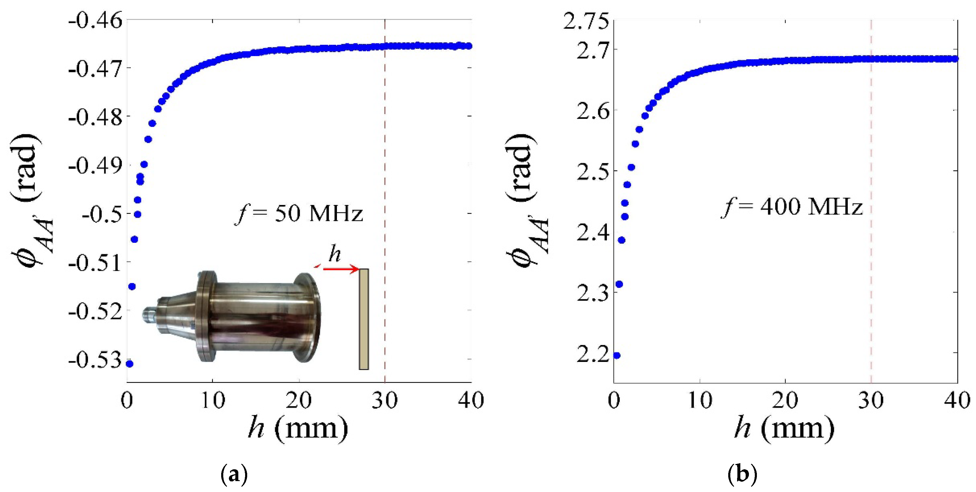
2.3. Probe Characterization Test
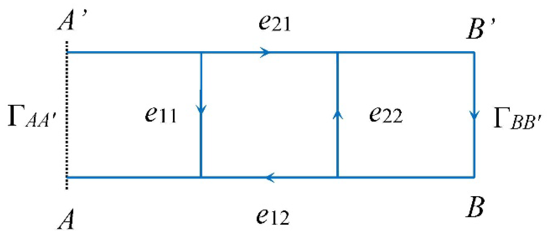
The complex reflection coefficient, ΓAA′ = |ΓAA′|exp(AA′) at plane AA′ for four MUTs were measured using Keysight E5071C network analyzer (Keysight Technologies, Santa Rosa, CA, USA) in the frequency ranging from 0.3 MHz to 650 MHz at 25 °C. Calibration was done at the AA′ plane, as shown in Figure 2, using Keysight 85032F kit (Keysight Technologies, Santa Rosa, CA, USA).
The sensing distance, h of the probe is 30 mm, which was estimated based on the distance at which the measured phase shift, φAA′ (rad) as shown in Figure 3a,b starts to become constant when the metallic plate is moved away from the probe aperture in air. Figure 4 shows the time-domain measurements of the coaxial probe, which is operated with minimum windowing and bandpass mode. Clearly, coaxial probe of 15 cm length is sufficient to avoid the interference between plane-AA′ and -BB′ for the frequency-domain ΓAA′ measurement.

3. Calibrations

3.1. Calibration Formulations

Before the one-port reflection measurement is conducted, the open-ended coaxial probe is regularly calibrated at the end of the coaxial line (probe aperture) in order to remove the effects of the coaxial line between AA′ plane and BB′ plane. The relationship between the actual reflection coefficient, ΓBB′ at the probe aperture (BB′ plane) and measured ΓAA′ can be represented by an error network as shown in Figure 5, and its formulation is given as [34]:
Γ B B = Γ A A e 11 e 22 Γ A A + ( e 12 e 21 e 11 e 22 )
where the e12e21 terms in Equation (2) represents the values of tracking error, as well as the e11 and e22 are the values of the directivity error and the source match error, respectively. These errors are contributed by shifted phase, attenuate loss in the coaxial line (e12e21), and the radiate fringing effects at the probe aperture (e11 and e22), which are mainly caused by the occurrence of standing waves in the coaxial line.
For simplicity of calibration process, only air independent calibration standard is considered in the de-embedded process. Thus, the errors of a standing wave and mismatch between connectors are not taken into account in the calibration, and the values of e11 and e22 are assumed to be zero. Finally, Equation (2) can be reduced as:
( e 12 e 21 e 11 e 22 ) = Γ A A _ A i r Γ B B _ A i r
where ΓAA′_Air is the reflection coefficient measurement, for air at plane AA′, and ΓBB′_Air is the standard value of the air reflection coefficient at plane BB′, obtained using the COMSOL simulator. Similarly, for MUT measurement, the Equation (2) can be expressed as:
( e 12 e 21 e 11 e 22 ) = Γ A A _ M U T Γ B B _ M U T
By combining Equations (3) and (4), the desired actual reflection coefficient, ΓBB′_MUT of the MUT can be obtained as:
Γ B B _ M U T = Γ A A _ M U T ( Γ B B _ A i r Γ A A _ A i r )
where ΓAA′_MUT is the reflection coefficient measurement, for MUT at plane AA′. Equation (5) can be converted in terms of normalized admittance parameter as given in Equation (12). It should be noted that the errors of e11 and e22 are implicitly removed by effective permittivity calibration process as described in Section 3.3.
In Ref. [32], the dependence of each capacitance on the MUT thickness, d at probe apperture as shown in Figure 6, is empirically assumed to be exponential as:
C 1 = ε r 1 C o [ 1 exp ( d / M ) ]
C 2 = ε r 2 C o exp ( d / M )
where M is an empirical parameter with the dimensions of length.
Thus, the total terminal capacitance, CT at BB′ plane can be written as:
C T = C f + C 1 + C 2 = C f + ε r 1 C o + ( ε r 2 ε r 1 ) C o exp ( d / M ) = C f + ε e f f C o
where εeff is the effective dielectric constant of finite layer MUT as:
ε e f f = ε r 1 + ( ε r 2 ε r 1 ) exp ( d / M )
However, Equation (9) is only valid for εr1′ > εr2′. For finite MUT with one layer thickness, d is backed by a conducting metallic plate (εr1′ < εr2′), the effective dielectric constant, εeff′ can be expressed as:
1 ε e f f = 1 ε r 1 + ( 1 ε r 2 1 ε r 1 ) exp ( d / M )
Since the dielectric constant of the metallic plate is assumed to be infinite (εr2′ ≈ ∞), therefore, the 1/εr2′ term in Equation (10) is neglected and subsequently yields
ε r 1 = ε e f f [ 1 exp ( d / M ) ]
In Ref. [35], Equation (11) was modified and expanded into Equation (15) by adding three unknown constants, a1, a2, and a3 (to be determined) in which the values of the constants are implicitly represented the e11 and e22 errors.

3.2. Probe Aperture Calibration

The actual normalized admittance, Y ˜ B B _ M U T , was measured with the aperture of the probe placed on a two-layer media [26], in which the first layered medium was a thin sample to be tested with thickness, h and the second layered medium was the conducting plate. The value of the Y ˜ B B _ M U T of the thin MUT is obtained after de-embedding using (13). The effective relative permittivity, εeff of the MUT can be estimated as [15]:
ε e f f = ( Y o j ω C ) Y ˜ B B _ M U T C f C
where
Y ˜ B B _ M U T = Y ˜ A A _ M U T ( Y ˜ B B _ A i r Y ˜ A A _ A i r )
where Y ˜ A A _ A i r is the measured normalized admittance for air at plane AA′, and Y ˜ B B _ A i r is the simulated standard value of admittance for air at aperture probe (plane BB′) using the COMSOL simulator as shown in Figure 7. In the simulation, the conductor of the coaxial probe is assumed to be a perfect conductor. The relationship between ΓAA′ and Y ˜ A A is given as:
Y ˜ A A _ M U T = 1 Γ A A _ M U T 1 + Γ A A _ M U T
Symbol Yo = 0.02 S, C = 2.38εo(ba) [36], Cf = 0.0107 pF and ω are the characteristic admittance, aperture probe capacitance, fringing field capacitance, and the angular frequency, respectively.

3.3. Effective Permittivity Calibration

For thin solid planar material measurements, the scattering of the wave from probe’s aperture would penetrate the thin planar material and impinge on the other layer-interface media. In this situation, the effective permittivity, εeff of the thin specimen will be measured, but not the actual permittivity, εr of the material [10]. In this study, the relationship between the actual relative permittivity, εr and effective relative permittivity, εeff for a finite thickness planar specimen was empirically expressed as Ref. [35]:
ε r = ε e f f ( a 1 + a 2 e h / M + a 3 e 2 h / M )
where h is the thickness of the MUT. The empirical coefficient, M was found to suite the large probe as described in Ref. [35], which can be roughly represented by single value as 0.006. The unknown complex coefficients (a1, a2, and a3) values in Equation (15) were found by using three offset-short terminators (εr = 1), yielding the following:
1 = ε e f f 1 ( a 1 + a 2 e h 1 / M + a 3 e 2 h 1 / M )
1 = ε e f f 2 ( a 1 + a 2 e h 2 / M + a 3 e 2 h 2 / M )
1 = ε e f f 3 ( a 1 + a 2 e h 3 / M + a 3 e 2 h 3 / M )
where h1, h2, and h3 are the known lift-off distances between the aperture probe from the shorted plate. On the other hand, εeff1, εeff2, and εeff3 are the corresponding effective permittivity of the three offset shorts, in which the values are obtained from (12). The unknown values of a1, a2, and a3 in Equations (16)–(18) were explicitly determined using Cramer’s rule as:
a 1 = { ( 1 / ε e f f 1 ) ( e ( h 2 + 2 h 3 ) / M e ( 2 h 2 + h 3 ) / M ) ( 1 / ε e f f 2 ) ( e ( h 1 + 2 h 3 ) / M e ( h 3 + 2 h 1 ) / M ) + ( 1 / ε e f f 3 ) ( e ( h 1 + 2 h 2 ) / M e ( h 2 + 2 h 1 ) / M ) } D
a 2 = { ( 1 / ε e f f 2 ) e 2 h 3 / M ( 1 / ε e f f 3 ) e 2 h 2 / M ( 1 / ε e f f 1 ) e 2 h 3 / M + ( 1 / ε e f f 3 ) e 2 h 1 / M + ( 1 / ε e f f 1 ) e 2 h 2 / M ( 1 / ε e f f 2 ) e 2 h 1 / M } D
a 3 = { ( 1 / ε e f f 3 ) e h 2 / M ( 1 / ε e f f 2 ) e h 3 / M ( 1 / ε e f f 3 ) e h 1 / M + ( 1 / ε e f f 1 ) e h 3 / M + ( 1 / ε e f f 2 ) e h 1 / M ( 1 / ε e f f 1 ) e h 2 / M } D
The determinant, D of the Equations (19)–(21) are given as:
D = { e ( h 2 + 2 h 3 ) / M e ( 2 h 2 + h 3 ) / M e ( h 1 + 2 h 3 ) / M + e ( h 3 + 2 h 1 ) / M + e ( h 1 + 2 h 2 ) / M e ( h 2 + 2 h 1 ) / M }
To perform offset-short measurements (Lift-off distances: h1, h2, and h3), three cylindrical rings have been printed using 3D-printer with polylactic acid (PLA) material in which the ring centers are concave rounded with depth, h1 = (1.0 ± 0.1) mm, h2 = (2.0 ± 0.1) mm, and h3 = (3.0 ± 0.1) mm, respectively. It should be noted that the effective lift-off distance may be slightly shorter than the actual physical distance due to the strong coupling fringing field near to the probe aperture. The cylindrical rings backed by aluminum plate as shown in Figure 8, are used as calibration kits for this thin planar material measurements. As mentioned earlier, a large aperture probe has a strong and wide fringing field distribution compared to a small probe, thus non-metallic material such as polylactic acid (PLA) has been chosen to construct the cylindrical ring in order to reduce the field coupling effect from side wall in the area between aperture probe and aluminum plate.

4. Results and Discussion

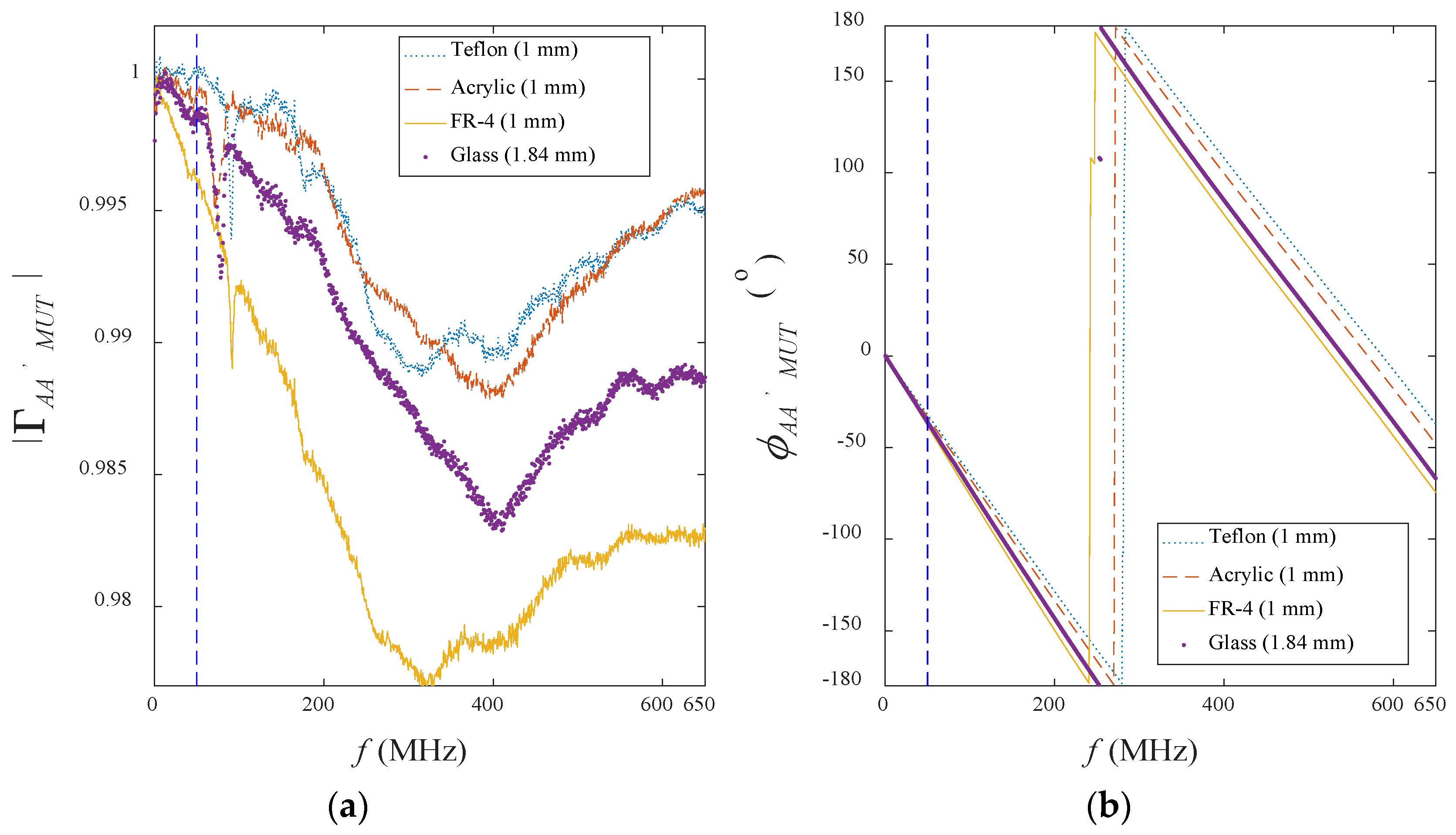
4.1. Reflection Coefficient, ΓAA′

Figure 9a,b shows the raw measured |ΓAA′_MUT| and φAA′_MUT data of four thin low-loss MUTs obtained from network analyzer. The |ΓAA′_MUT| and φAA′_MUT distinction between four MUTs are less significant when it is below 50 MHz, in which mainly caused by the size limitation of the coaxial probe. For instance, various coaxial probes (in Figure 10) are tested in order to observe and compare the measurement sensitivity towards the size of coaxial probe as listed in Table 2 and Table 3.
Up to five repeated reflection measurements (at different surface areas of the MUT) have been done for each MUT in which the average values and standard deviations for the measurement have been calculated. For this study probe, the linear magnitude differential, ∆|ΓAA′_MUT| between the RF-4 (h = 1.0 mm) and the Teflon (h = 1.0 mm) is close to 0.004 in which is ten time greater to the existing resolution error (standard deviation: 10−4) as shown in Table 2. On the other hand, the phase differential, ∆φAA′_MUT between FR-4 and Teflon at 50 MHz is capable of achieving 6° as illustrated in Table 3. Clearly, the larger the probe, the more stable and sensitive it can be achieved for reflection measurements at very low frequencies.

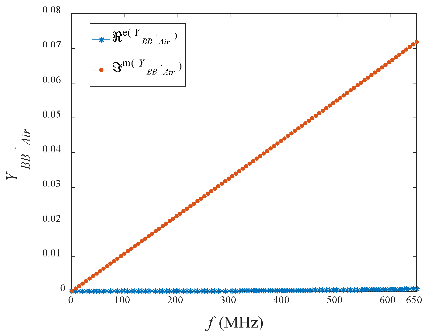
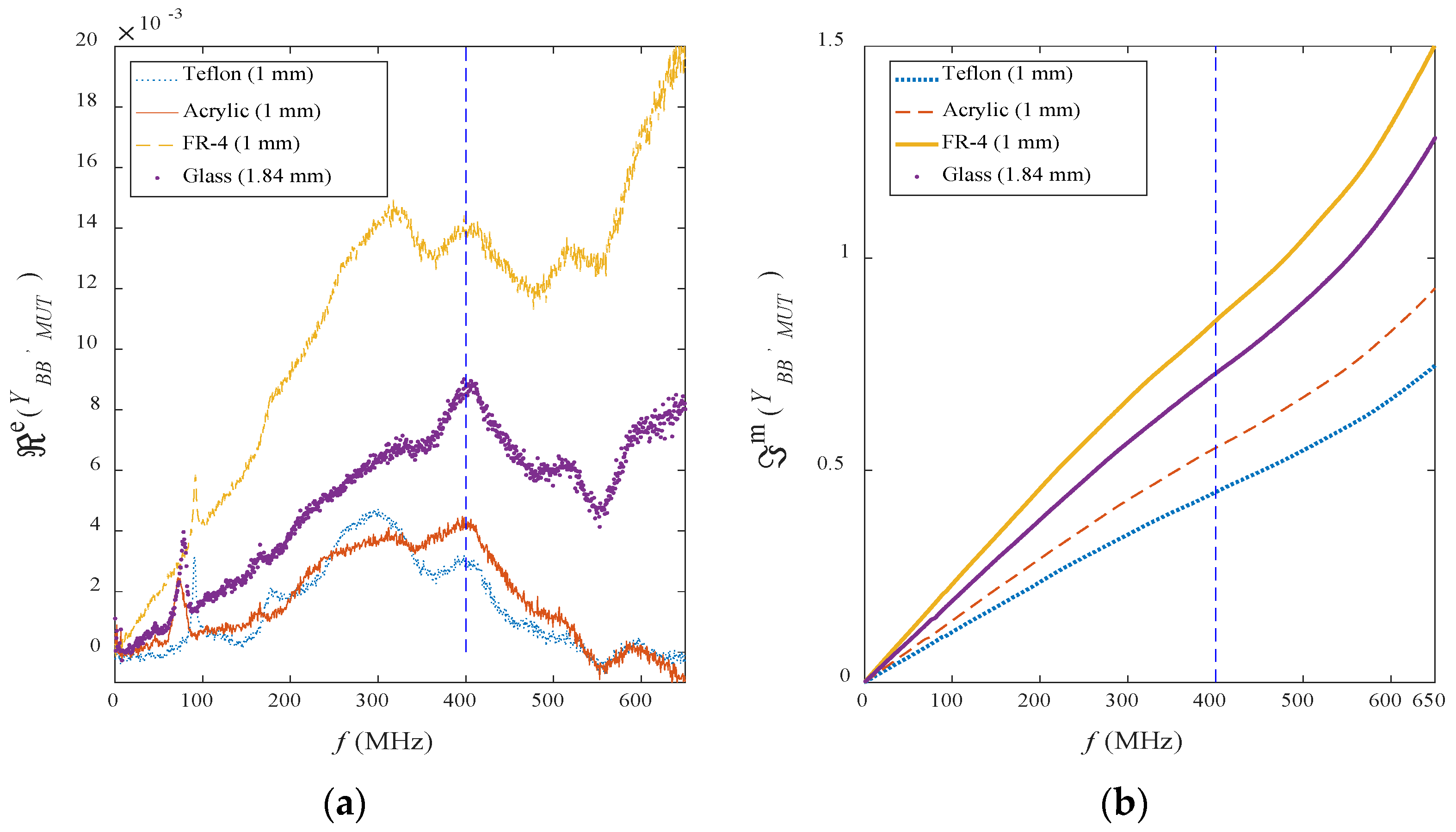
4.2. Normalized Admittance, ỸBB′

Figure 11a,b shows the normalized admittance Y ˜ B B _ M U T = ℜe ( Y ˜ B B _ M U T ) + j J m ( Y ˜ B B _ M U T ) of the four MUTs converted based on the raw ΓAA′_MUT data using Equations (13) and (14). Typically, the lower the loss for the MUT, the lower the value for real part, ℜe ( Y ˜ B B _ M U T ) (normalized conductance) as shown in Figure 11a. The case for the imaginary part, J m ( Y ˜ B B _ M U T ) (normalized susceptance) indicates that the J m ( Y ˜ B B _ M U T ) property is no longer linearly proportional to the operating frequency, f over than 400 MHz as shown in Figure 11b. Hence, the prediction of εr value will be less accurate because the model (11) used in the conversion assumed the value of J m ( Y ˜ B B _ M U T ) is proportional to the frequency.

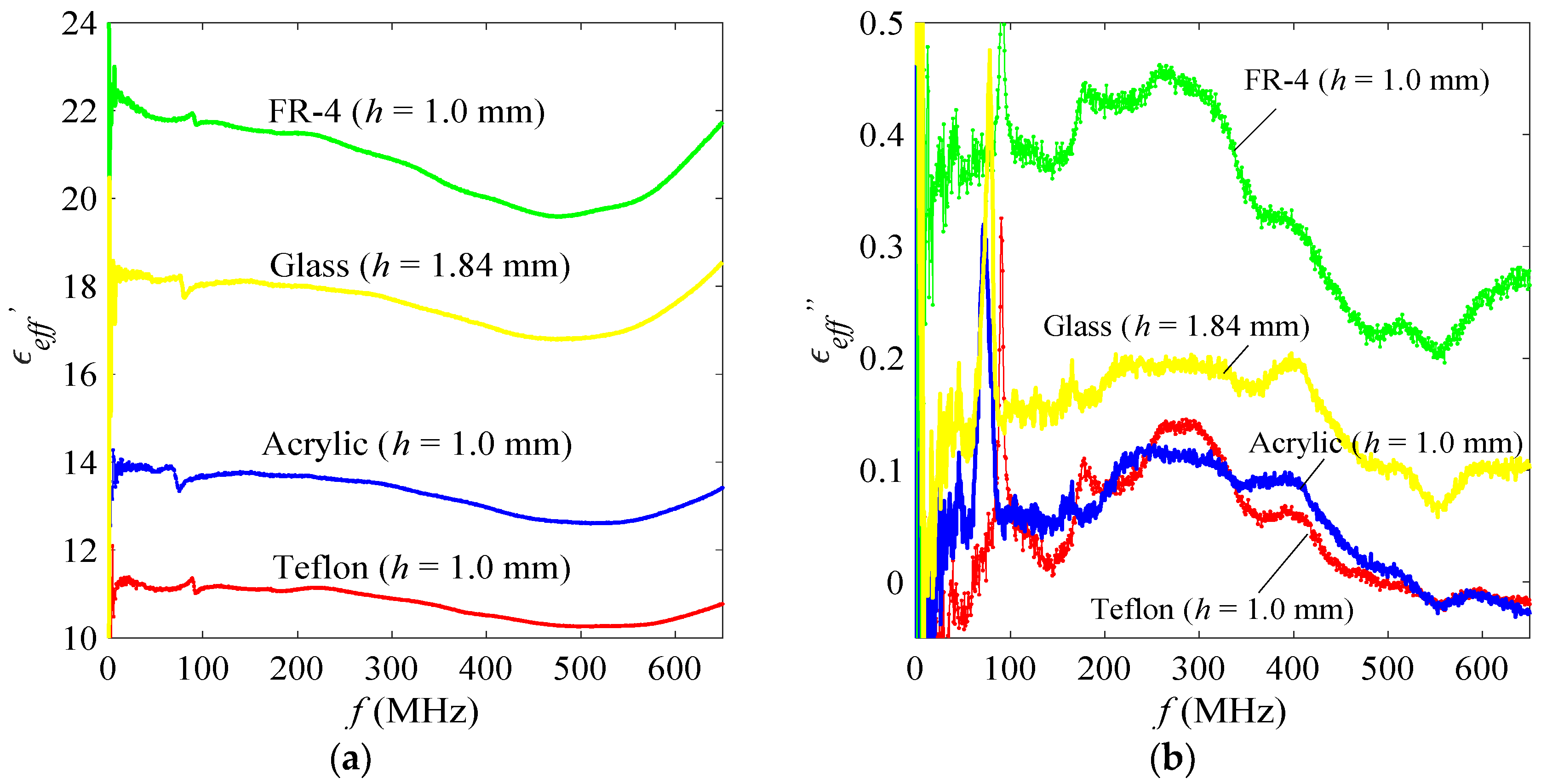
4.3. Effective Permittivity, εeff

Figure 12a,b shows the effective relative permittivity, εeff = εeff′ − eff″ versus operating frequency, f.
The value of εeff has been determined using Equation (12) and it is higher than the actual εr value of the MUT in which the εeff value is depended on the thickness, h of the MUT backed by metal plate. This is caused by the thinness of MUT at coaxial probe aperture, whereby the scattering of the wave from probe aperture will penetrate the MUT and coupling with the metal plate, as well as reflected by the metal plate on other side of the MUT [37].

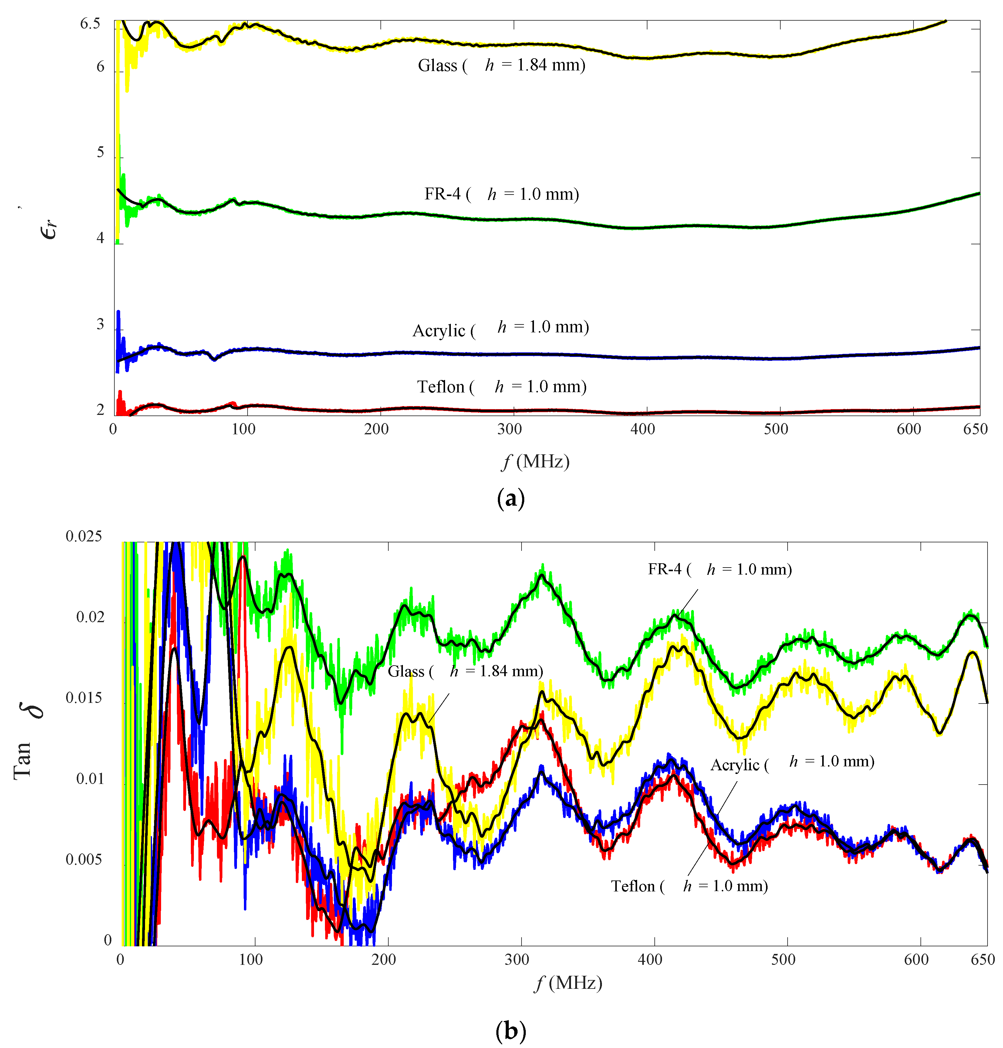
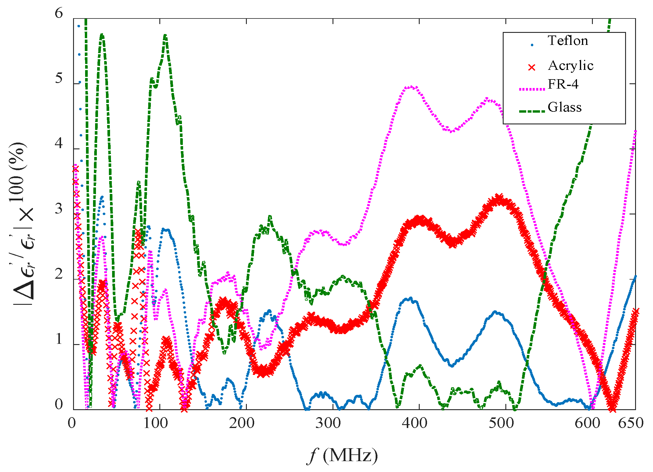
4.4. Actual Relative Permittivity, εr

Figure 13a,b shows the predicted εr′ and tan δ = εr″/εr′ of four thin low-loss MUTs which are in good agreement with expected values as tabulated in Table 2. The scattered εr′ and tan δ data in Figure 13a,b have been smoothed by Local Polynomial Regression (Loess) algorithm, which is available in built-in MATLAB “smooth” command. The smoothed data are represented by the black solid lines in Figure 13a,b. As expected, the coaxial probe is very difficult to provide high stability reflection measurement for the low-loss MUT at very low operating frequencies (refer to Figure 9). Hence, indirectly, the uncertainty of the predicted εr′ and tan δ (especially for small values of tan δ) are increased when the operating frequency decreases to below 50 MHz.
Figure 14 shows the percentage of the relative error between the smoothed values of εr′ in Figure 13a and the expected values of εr′ in Table 4. The percentage of the average relative errors, |∆εr′/εr′| are less than 6% for overall measurements from 1 MHz to 400 MHz.

5. Conclusions

One-port measurement using a large coaxial probe is an easy, durable, and cost-effective measurement method in large-scale material processing industries. In this study, the dielectric properties for thin low-loss materials (a few millimeter thickness) at very low frequencies (below 400 MHz) have been precisely measured using the open-ended coaxial probe techniques. This accuracy level of the measurement is rarely achieved by previous studies, which used the same technique for low-loss material at very low frequencies. In future, larger and longer sizes of coaxial probe may be re-designed in order to achieve good stability and higher sensitivity measurement below 50 MHz.

Author Contributions

Conceptualization, K.Y.Y.; Methodology, K.Y.Y.; Software, K.Y.Y.; Validation, M.S.S., and K.Y.Y.; Formal Analysis, K.Y.Y. and M.S.S.; Investigation, K.Y.Y. and M.S.S.; Resources, K.Y.Y.; Data Curation, K.Y.Y.; Writing—Original Draft Preparation, K.Y.Y.; Writing—Review and Editing, K.Y.Y.; Visualization, K.Y.Y.; Supervision, K.Y.Y.; Project Administration, K.Y.Y.; Funding Acquisition, K.Y.Y.

Funding

This research was funded by i-Stone Technology and Research University Grant (GUP) from Universiti Teknologi Malaysia under project number Q.J130000.2523.15H30 and the Ministry of Higher Education of Malaysia (MOHE).

Acknowledgments

Authors would like to thank to Kok-San Chan, Shau-Lim Ooi, Tze-Lok Eng, Cha-Heng Toh for their invaluable support in probe fabrication.

Conflicts of Interest

The authors declare no conflict of interest.

References

  1. Bakhshiani, M.; Suster, M.A.; Mohseni, P. A Broadband Sensor Interface IC for Miniaturized Dielectric Spectroscopy from MHz to GHz. IEEE J. Solid-State Circuits 2014, 49, 1669–1681. [Google Scholar] [CrossRef]
  2. Hegde, V.J.; Gallot-Lavallée, O.; Heux, L. Dielectric study of Polycaprolactone: A biodegradable polymer. In Proceedings of the 2016 IEEE International Conference on Dielectrics (ICD), Montpellier, France, 3–7 July 2016; Volume 1, pp. 293–296. [Google Scholar]
  3. Noh, J.; Kim, S.M.; Heo, S.; Kang, S.C.; Kim, Y.; Lee, Y.G.; Park, H.; Lee, S.; Lee, B.H. Time Domain Reflectometry Analysis of the Dispersion of Metal–Insulator–Metal Capacitance. IEEE Electron Device Lett. 2017, 38, 521–524. [Google Scholar] [CrossRef]
  4. Hewlett-Packard. User’s Manual: HP 85070B Dielectric Probe Kit; Hewlett-Packard Company: Palo Alto, CA, USA, 1997. [Google Scholar]
  5. Schmid & Partner Engineering, AG. High Precision Dielectric Measurements: DAK; SPEAG: Zurich, Switzerland, 2018. [Google Scholar]
  6. KEYCOM. Open Mode Probe Method Dielectric Constant and Dielectric Loss Tangent Measurement System; KEYCOM Characteristic Technologies: Tokyo, Japan, 2000. [Google Scholar]
  7. APREL. Dielectric Probe Kit ALS-PR-DIEL; APREL Inc.: Kanata, ON, Canada, 2014. [Google Scholar]
  8. Filali, B.; Boone, F.; Rhazi, J.; Ballivy, G. Design and Calibration of a Large Open-Ended Coaxial Probe for the Measurement of the Dielectric Properties of Concrete. IEEE Trans. Microw. Theory Tech. 2008, 56, 2322–2328. [Google Scholar] [CrossRef]
  9. Otto, G.P.; Chew, W.C. Improved Calibration of a Large Open-Ended Coaxial Probe for Dielectric Measurements. IEEE Trans. Instrum. Meas. 1991, 40, 742–746. [Google Scholar] [CrossRef]
  10. Damme, S.V.; Franchois, A.; Zutter, D.D.; Taerwe, L. Nondestructive Determination of the Steel Fiber Content in Concrete Slabs with an Open-Ended Coaxial Probe. IEEE Trans. Geosci. Remote Sens. 2004, 42, 2511–2521. [Google Scholar] [CrossRef]
  11. Huang, Y. Design, Calibration and Data Interpretation for a One-Port Large Coaxial Dielectric Measurement Cell. Meas. Sci. Technol. 2001, 12, 111–115. [Google Scholar] [CrossRef]
  12. Kitić, G.; Crnojević-Bengin, V. A Sensor for the Measurement of the Moisture of Undisturbed Soil Samples. Sensors 2013, 13, 1692–1705. [Google Scholar] [CrossRef] [Green Version]
  13. Busssey, H. Dielectric Measurement in a Shielded Open Circuit Coaxial Line. IEEE Trans. Instrum. Meas. 1980, 29, 120–124. [Google Scholar] [CrossRef]
  14. Brady, M.M.; Symons, S.A.; Stuchly, S.S. Dielectric Behavior of Selected Animal Tissues In Vitro at Frequencies from 2 to 4 GHz. IEEE Trans. Biomed. Eng. 1981, 28, 305–307. [Google Scholar] [CrossRef]
  15. Atley, T.W.; Stuchly, M.A.; Stuchly, S.S. Measurement of Radio Frequency Permittivity of Biological Tissues with an Open-Ended Coaxial Line: Part I. IEEE Trans. Microw. Theory Tech. 1982, 30, 82–86. [Google Scholar] [CrossRef]
  16. Gajda, G.; Stuchly, S.S. An Equivalent Circuit of an Open-Ended Coaxial Line. IEEE Trans. Instrum. Meas. 1983, 32, 506–508. [Google Scholar] [CrossRef]
  17. Kraszewski, A.; Stuchly, S.S. Capacitance of Open-Ended Dielectric-Filled Coaxial Lines-Experimental Results. IEEE Trans. Instrum. Meas. 1983, 32, 517–519. [Google Scholar] [CrossRef]
  18. Grant, J.P.; Clarke, R.N.; Symm, G.T.; Spyrou, N.M. A Critical Study of the Open-Ended Coaxial Line Sensor Technique for RF and Microwave Complex Permittivity Measurements. J. Phys. E 1989, 22, 757–770. [Google Scholar] [CrossRef]
  19. Levine, H.; Papas, C.H. Theory of the Circular Diffraction Antenna. J.Appl. Phy. 1951, 22, 29–43. [Google Scholar] [CrossRef]
  20. Nevels, R.D.; Butler, C.M.; Yablon, W. The Annular Slot Antenna in a Lossy Biological Medium. IEEE Trans. Microw. Theory Tech. 1985, 33, 314–319. [Google Scholar] [CrossRef]
  21. Misra, D. A Quasi-Static Analysis of Open-Ended Coaxial Lines. IEEE Trans. Microw. Theory Techn. 1987, 35, 925–928. [Google Scholar] [CrossRef]
  22. Anderson, L.S.; Gajda, G.B.; Stuchly, S.S. Analysis of an Open-Ended Coaxial Line Sensor in Layered Dielectric. IEEE Trans. Instrum. Meas. 1986, 35, 13–18. [Google Scholar] [CrossRef]
  23. Fan, S.; Staebell, K.; Misra, D. Static Analysis of an Open-Ended Coaxial Line Terminated by Layered Media. IEEE Trans. Instrum. Meas. 1990, 39, 435–437. [Google Scholar] [CrossRef]
  24. Xu, Y.S.; Bosisio, R.G. Nondestructive Measurements of the Resistivity of Thin Conductive Films and the Dielectric Constant of Thin Substrates Using an Open-Ended Coaxial Line. IEE Proc. H Microw. Antennas Propag. 1992, 139, 500–506. [Google Scholar]
  25. Li, L.L.; Ismail, N.H.; Taylor, L.S.; Davis, C.C. Flanged Coaxial Microwave Probes for Measuring Thin Moisture Layers. IEEE Trans. Biomed. Eng. 1992, 39, 49–57. [Google Scholar] [CrossRef]
  26. Jiang, G.Q.; Wong, W.H.; Raskovich, E.Y.; Clark, W.G.; Hines, W.A.; Sanny, J. Measurement of the Microwave Dielectric Constant for Low-Loss Samples with Finite Thickness Using Open-Ended Coaxial-Line Probes. Rev. Sci. Instrum. 1993, 64, 1622–1626. [Google Scholar] [CrossRef]
  27. Chen, G.; Li, K.; Ji, Z. Bilayered Dielectric Measurement with an Open-Ended Coaxial Probe. IEEE Trans. Microw. Theory Tech. 1994, 42, 966–971. [Google Scholar] [CrossRef]
  28. Li, C.L.; Chen, K.M. Determination of Electromagnetic Properties of Materials Using Flanged Open-Ended Coaxial Probe-Full-Wave Analysis. IEEE Trans. Instrum. Meas. 1995, 44, 19–27. [Google Scholar] [CrossRef]
  29. Ganchev, S.I.; Qaddoumi, N.; Bakhtiari, S.; Zoughi, R. Calibration and Measurement of Dielectric Properties of Finite Thickness Composite Sheets with Open-Ended Coaxial Sensors. IEEE Trans. Instrum. Meas. 1995, 44, 1023–1029. [Google Scholar] [CrossRef]
  30. Lee, J.H.; Eom, H.J.; Jun, K.H. Reflection of a Coaxial Line Radiating into a Parallel Plate. IEEE Microw. Guid. Wave Lett. 1996, 6, 135–137. [Google Scholar] [CrossRef]
  31. Folgero, K.; Tjomsland, T. Permittivity Measurement of Thin Liquid Layers Using Open Ended Coaxial Probes. Meas. Sci. Technol. 1996, 7, 1164–1173. [Google Scholar] [CrossRef]
  32. Alanen, E.; Lahtinen, T.; Nuutinen, J. Variational Formulation of Open-Ended Coaxial Line in Contact with Layered Biological Medium. IEEE Trans. Biomed. Eng. 1998, 45, 1241–1248. [Google Scholar] [CrossRef] [PubMed]
  33. Noh, Y.C.; Eom, H.J. Radiation from a Flanged Coaxial Line into a Dielectric Slab. IEEE Trans. Microw. Theory Techn. 1999, 47, 2158–2161. [Google Scholar] [CrossRef]
  34. You, K.Y. RF Coaxial Slot Radiators: Modeling, Measurements, and Applications; Artech House: Norwood, MA, USA, 2015; pp. 19–56. ISBN 9781608078226. [Google Scholar]
  35. You, K.Y.; Then, Y.L. Simple Calibration and Dielectric Measurement Technique for Thin Material Using Coaxial Probe. IEEE Sens. J. 2015, 15, 5393–5397. [Google Scholar] [CrossRef]
  36. Gajda, G.B.; Stuchly, S.S. Numerical Analysis of Open-Ended Coaxial Lines. IEEE Trans. Microw. Theory Techn. 1983, 31, 380–384. [Google Scholar] [CrossRef]
  37. Chen, L.F.; Ong, C.K.; Neo, C.P.; Varadan, V.V.; Varadan, V.K. Microwave Electronics: Measurement and Materials Characterization; John Wiley & Sons, Ltd.: West Sussex, UK, 2004; ISBN 9780470844922. [Google Scholar]
Figure 1. (a) Cross-sectional side view and dimensions (in mm) of the coaxial sensor. (b) Side view of the large coaxial sensor. (c) Internal configuration of the coaxial sensor.
Jmmp 02 00081 g001
Figure 2. Experimental set-up and measurement.
Jmmp 02 00081 g002
Figure 3. Variation in phase shift φAA′ with air thickness, h backed by metal plate at (a) 50 MHz and (b) 400 MHz.
Jmmp 02 00081 g003
Figure 4. The time-domain response for the end of cable at plane-AA′ with and without probe.
Jmmp 02 00081 g004
Figure 5. Error network.
Jmmp 02 00081 g005
Figure 6. Equivalent parallel capacitance model.
Jmmp 02 00081 g006
Figure 7. Simulated Y ˜ B B _ A i r = [ℜe( Y ˜ B B _ A i r ) + j J m ( Y ˜ B B _ A i r ) ] for air at aperture probe (plane BB′).
Jmmp 02 00081 g007
Figure 8. Printed offset short calibration kits.
Jmmp 02 00081 g008
Figure 9. Variation in (a) measured |ΓAA′_MUT| and (b) measured φAA′_MUT with frequency for the four materials under test (MUTs) at room temperature.
Jmmp 02 00081 g009
Figure 10. Various sizes of coaxial probe.
Jmmp 02 00081 g010
Figure 11. Comparison of (a) real part, ℜe ( Y ˜ B B _ M U T ) , and (b) imaginary part, J m ( Y ˜ B B _ M U T ) , of the normalized admittance at probe aperture for four MUTs.
Jmmp 02 00081 g011
Figure 12. Comparison of (a) real part, εeff and (b) imaginary part, εeff, of the effective relative permittivity, εeff for four MUTs.
Jmmp 02 00081 g012
Figure 13. Variation in (a) predicted εr′ and (b) predicted tan δ with frequency for the MUTs at room temperature.
Jmmp 02 00081 g013
Figure 14. Variation in % relative error of εr′.
Jmmp 02 00081 g014
Table 1. Comparative study of large probe.
Ref.Probe Size (cm)f (MHz)Transition SectionSample ContactSample Size/ShapeCalibration StandardsMeasured εr RangeInverse Method
[8]2a = 1.00
2b = 3.25
L = 5.00
100–900withoutAperture probeHalf-space infiniteAir, short, NaCl solution.~5–80Iterative
[9]2a = 1.00
2b = 3.25
L = 5.00
1–10 or
10–3000
withoutAperture probeHalf-space infiniteShort cavity orAir, short, short cavity~30–80 (Lossy)Iterative
[10]2a = 1.18
2b = 4.00
L ≈ 13.0
200–1500withAperture probeHalf-space infiniteAir, copper plate, Teflon plate.~2–35 (Lossy)Iterative
[11]2a = 4.50
2b = 10.3
L ≈ 41.0
50–1000withFilled in coaxial lineToroid-shaped3 positions short-circuit along the coaxial line~7–80 (Lossy)Iterative
[12]2a = 2.35
2b = 5.4
L ≈ 4.4
100–250withFilled in coaxial lineToroid-shapedBased on specified specimen under test1–50 (Low lossy)Non-iterative
This study2a = 1.50
2b = 4.80
L = 15.0
1–400withAperture ProbeThin planar backed by metal plateAir, 3 offset shorts1–20 (Lossless)Non-iterative
* L is the coaxial length of the probe.
Table 2. Measured |ΓAA′| for Teflon and FR-4 sheets with thickness of 1 mm backed by metal plate at 50 MHz.
Probe SizeAA′_MUT|Differentiation of ∆|ΓAA′_MUT| between Teflon and FR-4
TeflonFR-4
This study
2a = 1.5 cm
2b = 4.8 cm
1.000213Average: 1.0001019
Standard deviation: 0.0001784
0.9954108Average: 0.9959747
Standard deviation: 0.0004091
0.0041272
1.0003450.9961075
0.99994580.9957603
0.99992580.9964970
1.000080.9960977
Probe 1
2a = 0.3 cm
2b = 1.0 cm
1.001418Average: 1.001394
Standard deviation: 0.000155902
1.000593Average: 1.0005194
Standard deviation: 0.00010485
0.0008746
1.0015211.000355
1.0013021.000626
1.0011771.000507
1.0015521.000516
Probe 2
2a = 0.24 cm
2b = 0.8 cm
0.9998745Average: 0.9998884
Standard deviation: 0.000131850
0.9995621Average: 0.99951490
Standard deviation: 0.000038824
0.0003735
1.0000600.9994846
0.99988780.9995518
0.99992740.9994819
0.99969250.9994941
Probe 3
2a = 0.13 cm
2b = 0.42 cm
0.9996894Average: 0.99972804
Standard deviation: 0.000077999
0.9995004Average: 0.99967564
Standard deviation: 0.00014613
0.0000524
0.99962970.9995625
0.99984150.9998173
0.99973650.9998234
0.99974310.9996746
Probe 4
2a = 0.09 cm
2b = 0.3 cm
1.000269Average: 1.000275
Standard deviation: 0.000159385
1.000199Average: 1.0002248
Standard deviation: 0.000084138
0.0000502
1.0001831.000161
1.0003581.000366
1.0000751.000233
1.0004901.000165
Table 3. Measured φAA′_MUT for Teflon and FR-4 sheets with h = 1 mm backed by metal plate at 50 MHz.
Probe SizeφAA′_MUT (°) Differentiation of ∆φAA′_MUT between Teflon and FR-4
Teflon FR-4
This study
2a = 1.5 cm
2b = 4.8 cm
−32.3000Average: −32.21717
Standard deviation: 0.134307
−38.56207Average: −38.34329
Standard deviation: 0.495519
6.12612°
−32.13884−38.64224
−32.25762−38.43801
−32.02661−37.46768
−32.3628−38.60646
Probe 1
2a = 0.3 cm
2b = 1.0 cm
−1.943045Average: −1.93933
Standard deviation: 0.00692831
−2.522396Average: −2.542644
Standard deviation: 0.0144045
0.603314°
−1.930690−2.554037
−1.934963−2.535734
−1.939431−2.542843
−1.948521−2.558213
Probe 2
2a = 0.24 cm
2b = 0.8 cm
−13.88491Average: −13.884262
Standard deviation: 0.0098386975
−14.31968Average: −14.315222
Standard deviation: 0.00953097686
0.43096°
−13.89140−14.31454
−13.86970−14.32456
−13.89475−14.31788
−13.88055−14.29945
Probe 3
2a = 0.13 cm
2b = 0.42 cm
−1.426506Average: −1.4218634
Standard deviation: 0.00444004
−1.589263Average: −1.585402
Standard deviation: 0.00375146
0.163539°
−1.417838−1.579990
−1.419884−1.588442
−1.418287−1.583723
−1.426802−1.585592
Probe 4
2a = 0.09 cm
2b = 0.3 cm
−2.60528Average: −2.6106474
Standard deviation: 0.00985552
−2.71289Average: −2.688339
Standard deviation: 0.01568456
0.077692°
−2.60139−2.679226
−2.618748−2.694912
−2.623582−2.674806
−2.604237−2.679861
Table 4. Expected values for εr′ and tan δ.
MUTεr (Typ)tan δ (Max)
Teflon2.060.0004
Acrylic2.750.019
FR-44.40.022
Glass6.10.0036

