1. Introduction
Modern manufacturing demands high machining productivity and high accuracy. The unplanned maintenance and arbitrary failure of machine tools have a direct effect on the machining capability and accuracy of parts. Therefore, monitoring the machine tool state is a necessary part of modern manufacturing. Currently, a variety of approaches have been applied to machine tool condition monitoring. Regarding the significant failures of machine tools, they mostly monitor the machining process and mechanical structures of machine tools (feeding systems, tool changer, pallet and spindle system) by physical signals such as the vibration, power, current, acoustic emission, etc. [
1,
2,
3,
4]. The acquired signals are generally processed with the pattern recognition methods, such as neural networks, expert systems and fuzzy logic for condition monitoring and fault diagnosis [
5]. Currently, it is possible to measure the condition of some key elements of machine tools but it is not yet possible to measure the condition of all parts [
5]. Finding a signal which is related to more parts of the machine tool can provide a new look in machine tool condition monitoring. The condition of most machine tool elements can be reflected in the means of machine tool accuracy parameters. However, the machine tool accuracy information frequently measured during the maintenance period of machine tools are rarely used for continuous condition monitoring of machine tools. In addition, the measurement of geometric errors is generally a time-consuming process.
Volumetric errors (VE) are related to the machine tool mechanical structures and components such as the linear and rotary axes. They are the comprehensive reflections of machine tool quasi-static errors and hysteresis errors. As an important indicator of machine tool performance, its use for monitoring the machine tool accuracy states appears relevant. For the application of VE, currently, most works have been found in VE modelling, estimation and its compensation [
6,
7,
8,
9,
10,
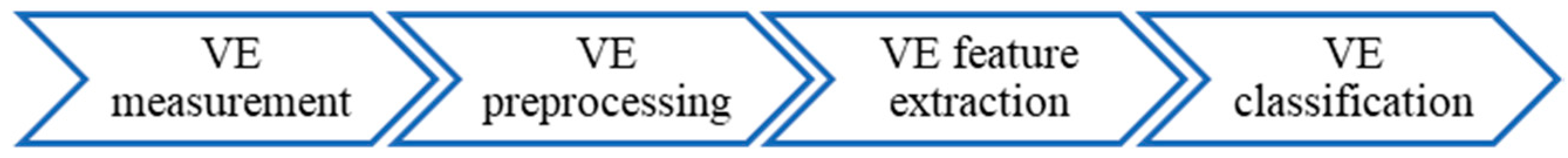
11]. Rarely research about VE has been seen in machine tool condition monitoring. The application of VE in machine tool condition monitoring includes two main parts—VE features extraction and VE data classification.
For the signal processing, feature extraction is one important step for the condition monitoring system. Features are any parameters extracted from the measured VEs to expel the effect from the random noises in the error measurement through signal processing methods. Feature selection is helpful to reduce dimensionality and discard deceptive features. It is even critical to the success of the VE classification. If the VE feature extraction is incorrect or incomplete and it will inevitably lead to erroneous classification and false positives. The general feature extraction methods include independent component analysis, principle component analysis (PCA), nonlinear principal components analysis. etc. [
12]. PCA is an unsupervised automatically feature extraction technique. It was first proposed to decorrelate the statistical dependency between variables in multivariate statistical data [
13]. Since then, it has been widely applied in areas such as statistical analysis, process monitoring and diagnosis and pattern recognition [
13]. PCA is a simple nonparametric method which can extract the most relevant information from a set of redundant or noisy data and form some new variables, the principal components, and explained the maximum amount of variability of the original data. In the area of machine condition monitoring, PCA method has been investigated to identify the most representative features from a variety of characteristic features of roller bearings and gearbox in time, frequency and or time-frequency domains [
14,
15]. The effectiveness of PCA has been verified experimentally on a bearing test machine, the results validated the suitability of the PCA features selection scheme [
14]. With reference to geometric tolerances, PCA can reveal the signatures of machined items in the manufacturing [
16]. As for the machine tool thermal monitoring, PCA has proved able to extract the features from eight fiber Bragg grating signals and six thermal signals with data dimensionality reduction [
17]. This is useful in processing a large amount data in real-time or in a long period of time. When using the force signature for the failure detection in assembly, PCA can compress the force signature and as a result reduce the number of examples required for mathematical modelling [
18]. For machine tool thermal errors compensation, PCA has allowed to select the optimization data of the temperature measurement points with dimension reduction of temperature data from 11 down to 4 [
19].
Clustering can assign a set of objects into different groups so that the objects in the same cluster are more similar to each other. It plays an important role in data analysis and pattern classification. Clustering techniques can be classified as hierarchical clustering, partitional clustering, graph theory based clustering, fuzzy based clustering or neural networks based clustering, etc. [
20]. As a squared error-based clustering method, the K-means algorithm can not only be simply implemented in solving many practical problems but also can be applied directly to industrial environments without the need to be trained by data measured on a machine under a fault condition [
20,
21,
22]. As an unsupervised method, K-means has been used to detect faults in rolling element bearing and used in the crack fault classification for planetary gearbox [
23]. In addition, it has been used to investigate the best signals from force, electrical current, and electrical voltage for a condition monitoring system. In summary, K-means is a good tool for monitoring systems in fault classification. Therefore, it is selected for the VE features classification.
In this research, VE has been firstly used to monitor the machine tool accuracy condition. For the VE data processing, we explore how to apply the PCA method to extract VE features and use the K-means method to classify the machine tool states indicated by these features. The results are the preliminary work with a scope to be extended further for a VE based condition monitoring solution in the future. The novelty of this paper lies in the development of an effective tool for VE features extraction and classification. The paper begins by presenting the state-of-the-art in machine tool condition monitoring, PCA and K-means clustering methods.
Section 2 presents the knowledge of volumetric error of machine tools. The VE measurement and processing plan is described in detail in
Section 3. After that, the VE data source for this research is introduced in
Section 4. The processing results of PCA and K-means in VE data are analyzed and discussed in
Section 5 and, finally, the conclusions are drawn in
Section 6.
2. Volumetric Error
Volumetric errors (VEs) are affected by a wide range of machine components which make them potentially able to provide a broad view of the machine condition. Machine tool VEs come from quasi-static errors including geometric errors, elastic, thermo-mechanical errors and hysteresis errors which come from manufacturing, assembly, loads, motion control and control software. VE components are caused by individual machine axis errors whereas others are related to the relative location of axes.
In this paper, VE is defined as the relative Euclidian error vector between the tool frame and the workpiece related frame in 3D space [
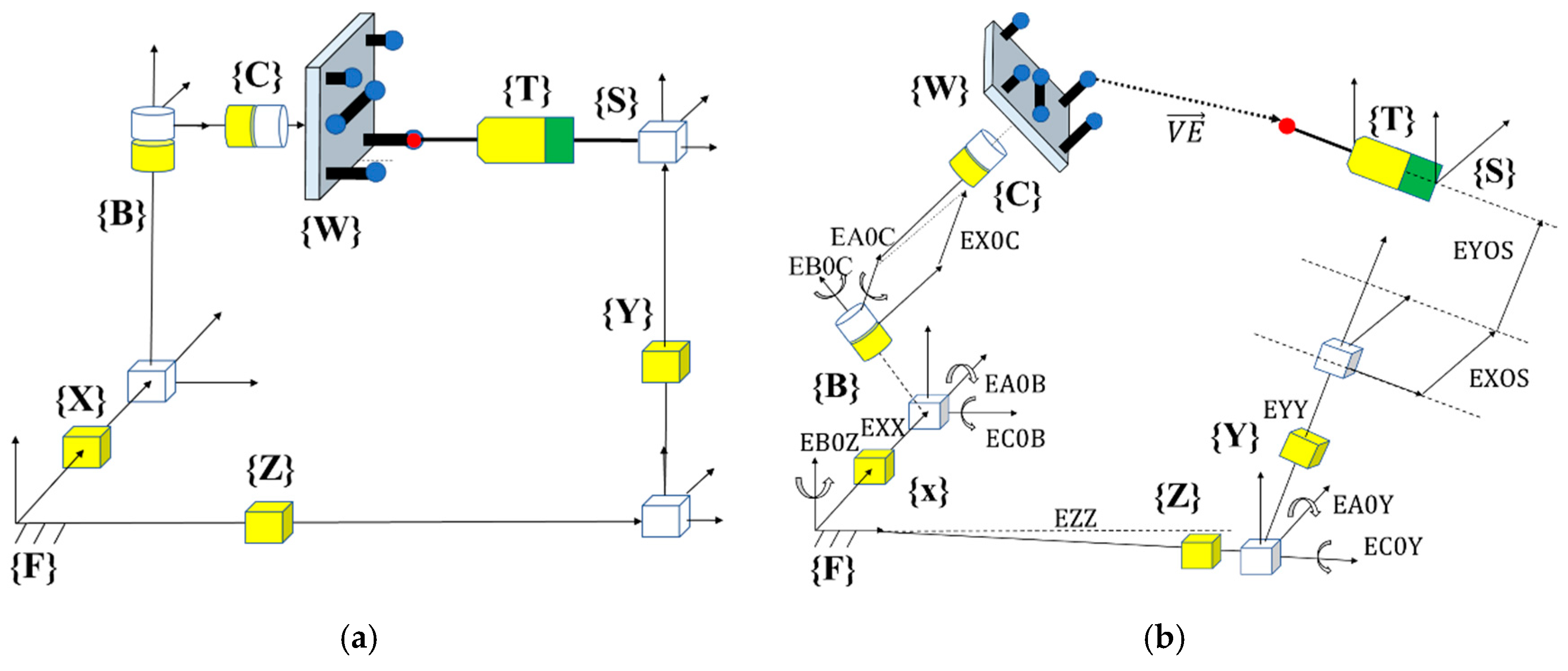
9]. The tested machine is a Mitsui Seiki HU40-T 5-axis machine tool (Mitsui Seiki (USA) Inc., New York, NY, USA), with three linear axes (X, Y, Z) and two rotary axes (B, C) and it has the topology WCBXFZYST where S stands for the spindle, W for the workpiece, F for the foundation, and T stands for the touch trigger probe (
Figure 1a). For the nominal machine tool model, the measure provided by the machine axis readings will correspond to the stylus tip position when it corresponds to the center of the master ball. However, owing to the presence of quasi-static errors (
Figure 1b), there will be a “mismatch” between the center of the probe and the master ball artefact. The “mismatch” between the calculated coordinates of the master ball artefact and the touch probe stylus tip coordinates represents the raw volumetric information that contains the accuracy information of the machine tool.
3. VE Measurement and Processing Plan
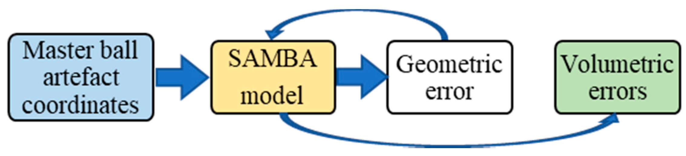
The functional information flow of the VE data processing is shown in
Figure 2. During the machine tool maintenance period, accuracy measurement devices/methods will be run to acquire the VE data. Then, PCA is used to extract the VE features from the preprocessed VE data. The VE features are classified by the K-means to check the states of machine tool indicated by the VE. After that, the change of the states of the machine tool can be revealed for maintenance decision purposes.
3.1. VE Measurement Method
VE measurement methods include ball-bar test, R-test, laser tracker quadrilateration, machining tests and the scale and master ball artefact (SAMBA) method, etc. [
24,
25,
26]. We chose to use the SAMBA method to estimate the VE in this research because of its advantages in terms of its simple installation and maintenance, automated data acquisition and processing [
24]. In addition, using the SAMBA method, only 30 min are needed for the measurement and estimation of geometric errors and VEs. This promotes the monitoring of VE as a faster alternative for machine tool accuracy condition monitoring.
The SAMBA method assumes that the rigid body kinematics hypothesis applies and so the machine is modelled using a series of homogeneous transformation matrices incorporating nominal axis locations and their location errors as well as the perfect axis motions of individual axes and their error motions. The “13” and “84” machine error models are the two SAMBA models which can estimate the VE and geometric errors. The naming of the two models is derived from the number of estimated machine error parameters. The “13” machine error model can estimate 13 machine error parameters namely the eight axis location errors (according to the standard ISO 230-1 [
27]) such as EA0B, EC0B, etc., three linear gains (EXX1, EYY1, EZZ1) and two spindle offsets (EY0S, EX0S). The “84” machine error model can estimate 26 types of machine errors of linear and rotary axes which are expressed with third-degree polynomials for a total of 84 coefficients. Some errors such as EAY, EBY and ECY errors are not distinguishable from EXY, EYY, and EZY, they are, therefore, not included in the “84” machine error model.
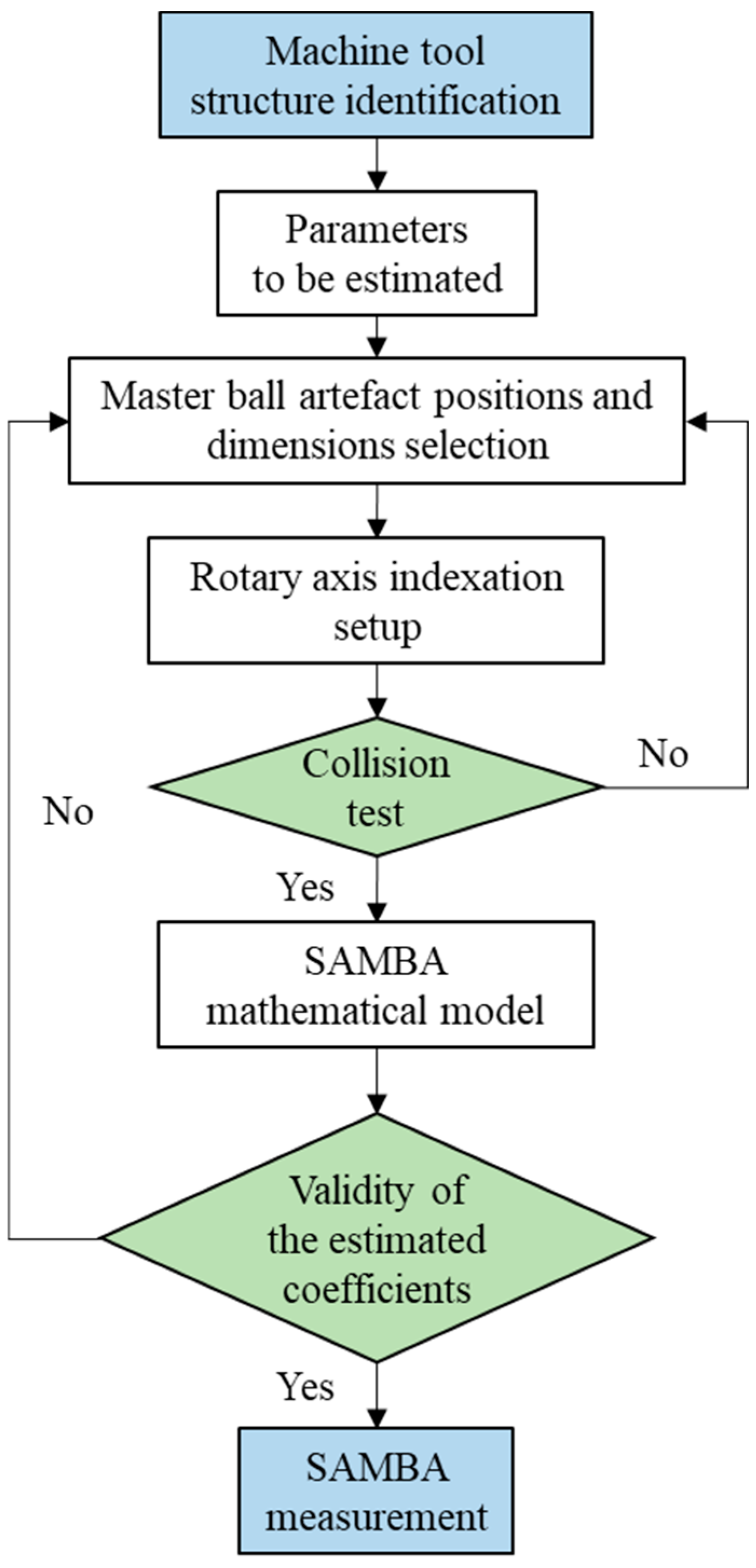
The steps of the SAMBA method are shown in
Figure 3. Machine tool’s actual kinematic model is firstly estimated. Considering the user’s requirements such as error types (inter or intra axis error), total measurement time, a machine error model needs to be firstly selected. After that, the error which are either those of the “13” machine error model or of the “84” machine error model can be automatically selected. The total number of machine error parameters helps to select the number of possible master ball positions and indexations (the relative positions of all rotary axis). Then, a collision test will be processed using the simulation method in VERICUT software (CGTech Ltd., Irvine, CA, USA). The indexations and the positions of master ball artefacts need to be optimized until there is no collision. The master ball artefacts and scale bar artefact installed on the machine tool pallet are probed, in simulation, by the touch trigger probe which is installed in the spindle under different indexations sets of the rotary axis. Then, all the setup parameters including the machine error parameters, indexation and the master ball artefacts to be probed in each indexation will be inputted into the SAMBA mathematical model to calculate the conditioning number and rank of the mathematical model. When the two values are deemed within acceptable limits, the proposed measurement plan can be applied to the real machine tools.
In this research, the “13” machine error model is selected to estimate the geometric errors and VEs. Four master ball artefacts and one scale bar artefacts are mounted, and 13 indexations are selected to accumulate the master ball center coordinates from 29 VE measurement positions. These measured master ball coordinates inputted into the SAMBA model are firstly used to estimate the machine error parameters of machine tool (
Figure 4). Then, under the SAMBA model, the estimated geometric error parameters are used for the estimation of VE.
where
is the volumetric error column matrix at the measured joint positions in the tool frame,
is the Jacobian matrix generated for the “13” machine error model describing the sensitivity of the observed volumetric deviations to the machine error parameters and
is the machine error parameters having 13 rows. For details of the SAMBA method in VE estimation, please refer to [
24,
26,
28].
3.2. VE Preprocessing
After the VE measurement, the measured VE data needs to be preprocessed for later VE feature extraction and classification. The estimated VE is written as
. Then each VE vector is processed by a vector similarity measure, the module parameter (Equation (2)):
The basic VE dataset of one measurement cycle can be written as where = 1 to 29 and it stands for the jth VE measurement position. For periodic monitoring cycles, the VE data can be expressed as where i represents the VE measurement time. It contains all the VE information.
3.3. VE Feature Extraction
The basic concept behind PCA in VE feature extraction is to project the VE dataset onto a subspace of lower dimensionality. In the reduced space, the VE data are represented with the removed or greatly decreased collinearity by explaining the variance of the preprocessed
in terms of a new sets of independent variables. In this paper, we will not discuss the mathematical details of PCA, but more details can be found in [
13]. The VE feature extraction is easily processed with program developed by Matlab (MathWorks Inc., Natick, MA, USA). The general steps of PCA in VE data feature extraction are as follows:
1. VE data preparation. The preprocessed
is prepared as the input of the PCA model. VE data size can affect the performance of PCA. Small sample data manifests itself in factors that are specific to one data set. This can bring large sampling errors to the PCA results. However, there is no absolute standard for the minimal size or subject to item ratio of data for PCA application, but large sample size or subject to item ratio are always recommended [
29]. Subject to item ratio is defined as the ratio of the total VE testing times (67) and VE measurement positions (29) in one test, it is 2.3 for this research, similar application of the subject to item ratio (55/22) could be found in [
30].
2. The
is used to create a new normalized matrix
. This is a necessary step for the VE data processing because the VEs measured in 29 positions have different magnitudes (from 1.2 µm to 164 µm). Otherwise, the magnitudes of certain VEs dominate the connections between the VEs in the sample. The normalization is carried out in each row
j with Equation (3):
3. Calculate the covariance matrix
of the new normalized matrix
:
4. Calculate the eigenvalues and eigenvectors of the covariance matrix
.
(
j = 1, 2, 3, …, n) are the eigenvalues and they are sorted in descending order,
(
P = 1, 2, 3, …, n) are the corresponding eigenvectors. The eigenvectors corresponding to the largest eigenvalues would bring the smallest errors in new feature representation. In addition, the maximum variance could be found in the direction of the eigenvectors:
5. Choose the components by considering the cumulative percent variance (CPV) which denotes the approximation precision of the new largest eigenvectors which account for all the variation of the raw VE data
. The number of principal components which need to be extracted is determined by the principle that the CPV value is more than 85%:
where
is the
Pth eigenvalue of the covariance matrix. The first N largest eigenvalues are retained in the PCA model.
6. Calculate the final projected data set which represents the modelled variation of
based on the first N components. The initial data set
is finally projected onto a new structure with new sets of data matrix
, where
is the matrices of N retained eigenvectors:
The final selected N components will be selected as the inputs of K-means for VE features classification.
3.4. VE Features Classification
K-means is a vector quantization method for cluster analysis. It has been widely adopted in scientific fields due to its ease of implementation, simplicity and efficiency in application [
31]. The main aim of K-means clustering in VE feature classification is to classify machine tool accuracy states into different clusters by analyzing the VE features extracted by PCA. The observation
groups using an iterative process that begins with the random assignment of a cluster to each data point. Then, the data are rearranged within the clusters by assigning them to the nearest cluster center. Finally, VE data measured from the machine tool with the same condition can be grouped together. The flowchart of the K-means in VE feature classification is divided into 6 steps:
Step 1: Prepare the VE feature data .
Step 2: Randomly select K cluster center setups (1 ≤ n ≤ K). This setup can guarantee no empty cluster appears after initial assignment in the subroutine.
Step 3: Calculate the Euclidean Distance between each data object (1 ≤ a ≤ i) and all K cluster centers (1 ≤ n ≤ K) and assign each data object to the nearest cluster.
Step 4: Update the K cluster center at periodic intervals after all VE features have been assigned.
Step 5: Repeat steps 2 to 4 until there is no change in the sum value of the total squared errors (
SSE) for each cluster center. After this process, the VE features could be separated into different groups:
Step 6: Reveal the classification results of VE features in a 2D figure.
According to the above algorithm principle, MATLAB, one kind of engineering calculation software, is used to develop the program of VE feature classification by K-means. The selection of K value directly affects the final classification. K-means is significantly sensitive to the initial cluster number. Owing to the random selection of K value, different classification results can be achieved. Several methods can be used as a reference for K value selection. It can either be selected based on the user’s knowledge of the dataset, the elbow method, the silhouette method, or even using a systematic approach which assigns the K value in the range
, where
i = 67 is the VE measurement times [
32,
33,
34].
4. VE Data Source for This Research
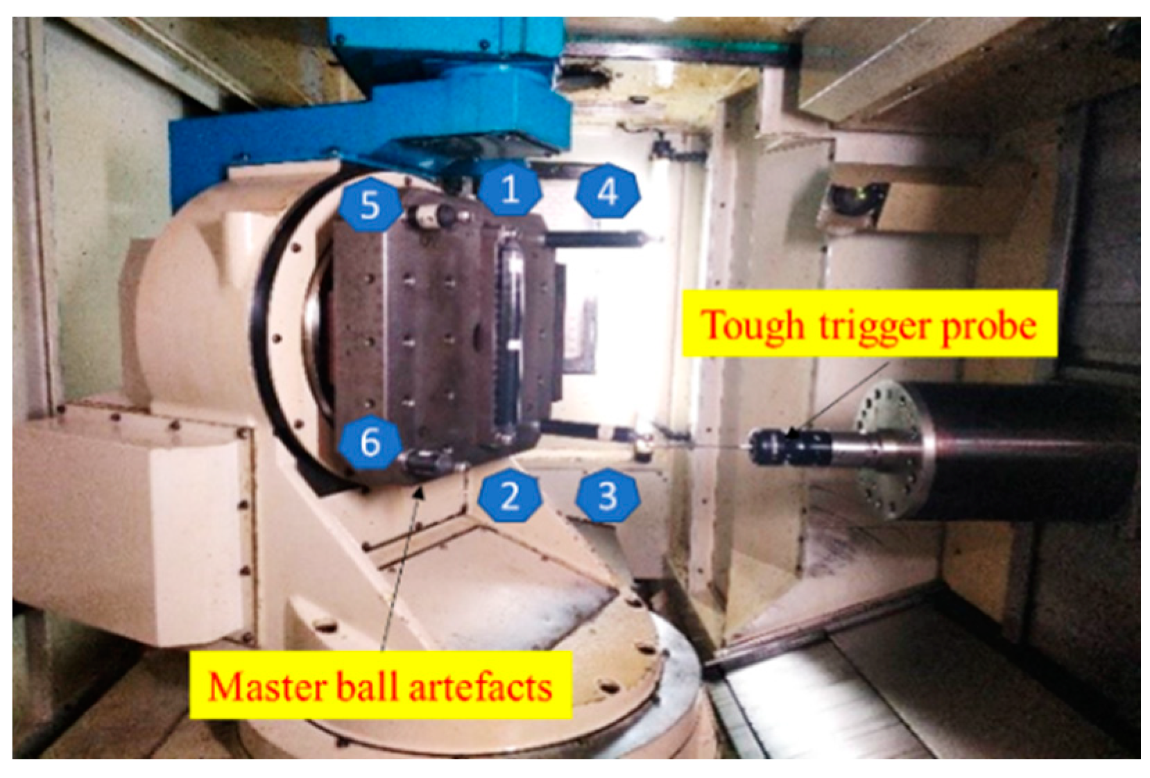
The SAMBA test is carried out on the Mitsui Seiki HU40-T five-axis machine tool (Mitsui Seiki (USA) Inc. New York, NY, USA) fitted with a MP700 Renishaw touch trigger probe (Renishaw, Inc. Wotton-under-Edge, UK) on the spindle and four master ball artefacts and one scale ball bar (Laboratoire de recherche en fabrication virtuelle, Polytechnique Montréal, Montréal, Canada) on the pallet (
Figure 5). The positions of the artefacts are measured by the probe with B and C axes in 13 different indexations (different angular position pairs). The measured 29 master ball artefact center coordinates are used as the inputs of the SAMBA mathematical model (the “13” machine error model). For each test, 29 VE vectors can be estimated. The machine tool has been periodically tested twice times per week at an ambient temperature of 21 ± 1 °C. Finally, 67 cycles of VE measurements are selected for this research.
The experimental machine tool experiences five different states during the SAMBA measurement (
Table 1): normal state 1, fault state 1 (C axis encoder fault), fault state 2 (uncalibrated C axis encoder fault), and fault state 3 (pallet location fault), and another normal state 2 after fixing all the mentioned faults. Normal state 1 and normal state 2 are viewed as the similar states of the machine tool without any faults.
5. Result and Discussion
5.1. VE Feature Extraction
The VE data are preprocessed with the Module measure. Then, the processing result
will be processed by PCA.
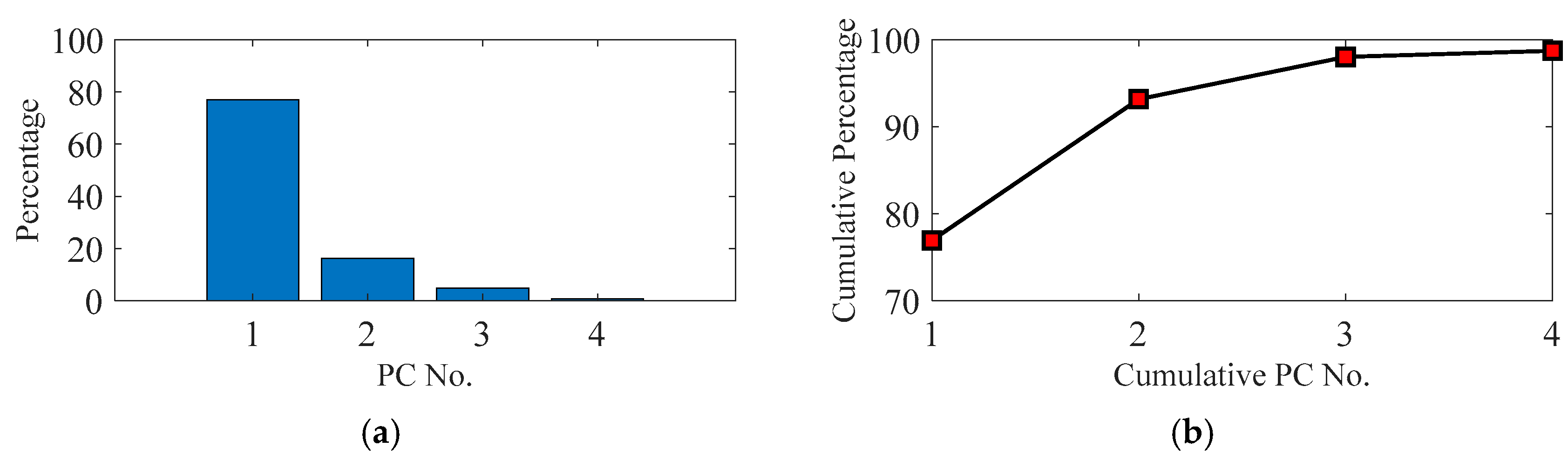
Figure 6 illustrates the contribution rate of the four main principal components (PCs) to the VE data. The 5th to 29th PC contributes less than the 4th PC to the VE data, so they are not shown in
Figure 6. The four components account for 98% of the measured VE data information. Although the four new PCs account for the most percentage of the VE data, they are not all efficient for the machine tool accuracy states recognition.
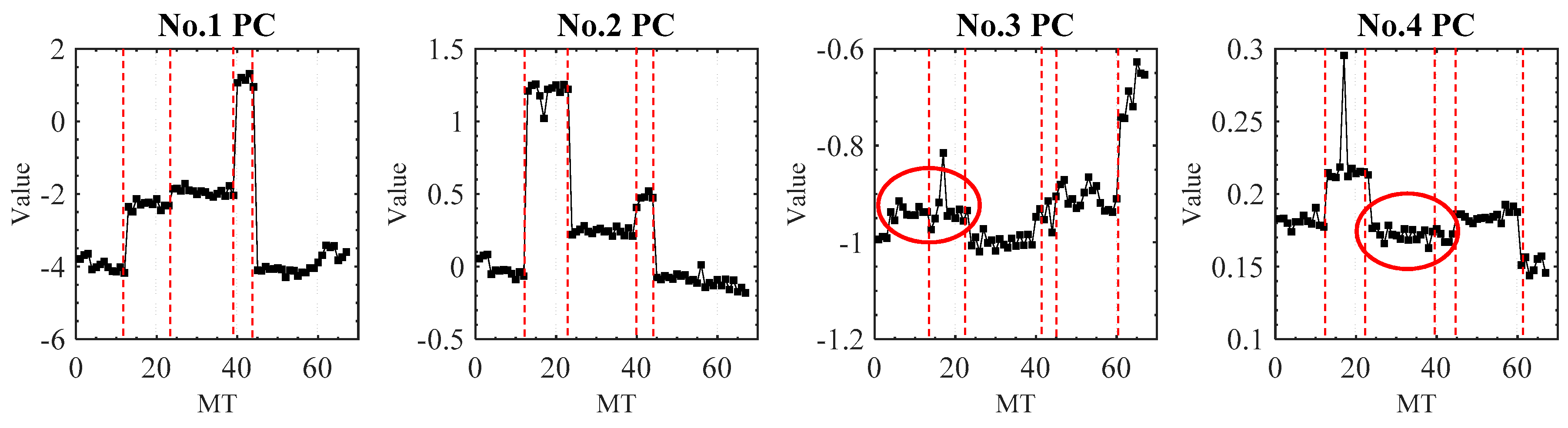
Owing to the differences of the contribution rate, each component performs differently in machine tool states reflection. For the PC selection, firstly, the CPV value needs to be larger than 85%. So, at least two components need to be selected (
Figure 6b). Secondly, the selected PCs need to reflect the main states of the machine tool without adding noisy information. The first and the second PCs can identify the five states of the machine tool (
Figure 7).
However, the remaining two principal PCs are unable to separate the transition of machine tool states and their curves do not have a similar change tendency. Two separate states (red ring, normal state 1 and fault state 1, fault state 2 and fault state 3) of the PC3 and PC4 are merged together. Therefore, the third and fourth PCs would probably add unnecessary noise to the machine tool state recognition. So, only the first and second PCs are extracted as the new features of VE in this research. They account for a total of 92.1% of the input VE data. After the PCA processing, the dimension of the original VE data is, therefore, decreased from 67 × 29 to 67 × 2.
5.2. VE Feature Classification
5.2.1. K Value Selection
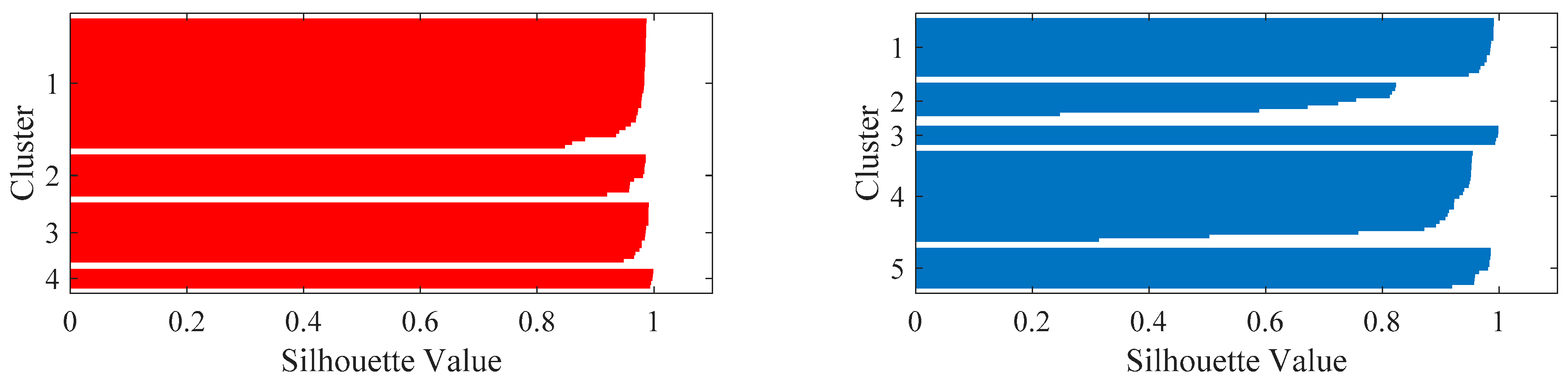
After the PCA processing, the first and second PCs are processed with the K-means method for feature classification. As mentioned above, elbow and silhouette methods are used for the K value selection. The Elbow method is a visual method. It starts with K = 2 and keeps increasing it in each step by 1, calculating the clusters and the sum of squared errors (SSE) of each classification. Then, SSE curve is plotted with the number of clusters K. The location of a bend (knee) in the plot is generally considered as the indicator of the appropriate number of clusters. To improve the precision of K value selection, Elbow method is firstly applied, after that, the silhouette method is used to verify the selection result. The silhouette coefficient has a range of [−1, 1]. +1 indicates that the sample is far away from the neighboring clusters, so the classification is good. A value of 0 indicates that the sample is on or very close to the decision boundary between two neighboring clusters and negative values indicate that those samples might have been assigned to the wrong clusters.
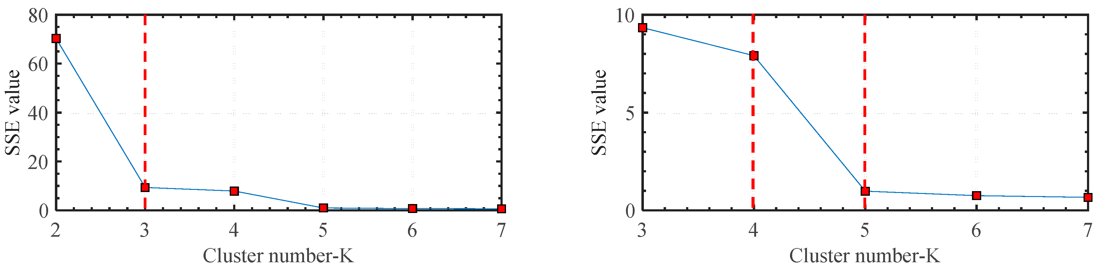
Figure 8 reveals the change tendency of
SSE with different K values. With the increase of K value,
SSE decreases gradually. Cluster number 3, number 4, and number 5 can each be deemed as the knee point because a large change can be found between cluster numbers 2 and 4, cluster numbers 3 and 5, and cluster numbers 4 and 6. For cluster number 3, it does not match the actual states of the machine tool. Thus, cluster number 3 is not considered. For the selection of cluster numbers 4 and 5, the silhouette values of the two-cluster number should be calculated.
Figure 9 illustrates the silhouette value of the K-means classification plan with K = 4 and K = 5. By checking the silhouette values of the two-classification plan, most of them are bigger than 0.2 and close to 1. However, the silhouette values of the classification plan with K = 4 are larger than those of the other classification plan with K = 5. Therefore, K = 4 is the recommended value for the classification of the VE data obtained by the elbow and silhouette methods.
However, the measured VE data contains two normal states and three fault states. This indicates that one of the clusters of the classification plan with K = 4 contains the components which are classified in two different clusters in the classification plan with K = 5. To see the differences between the normal state 1 and normal state 2, the K-means classification plan with K = 4 and 5 has been both tested in this research.
5.2.2. Classification Results Analysis
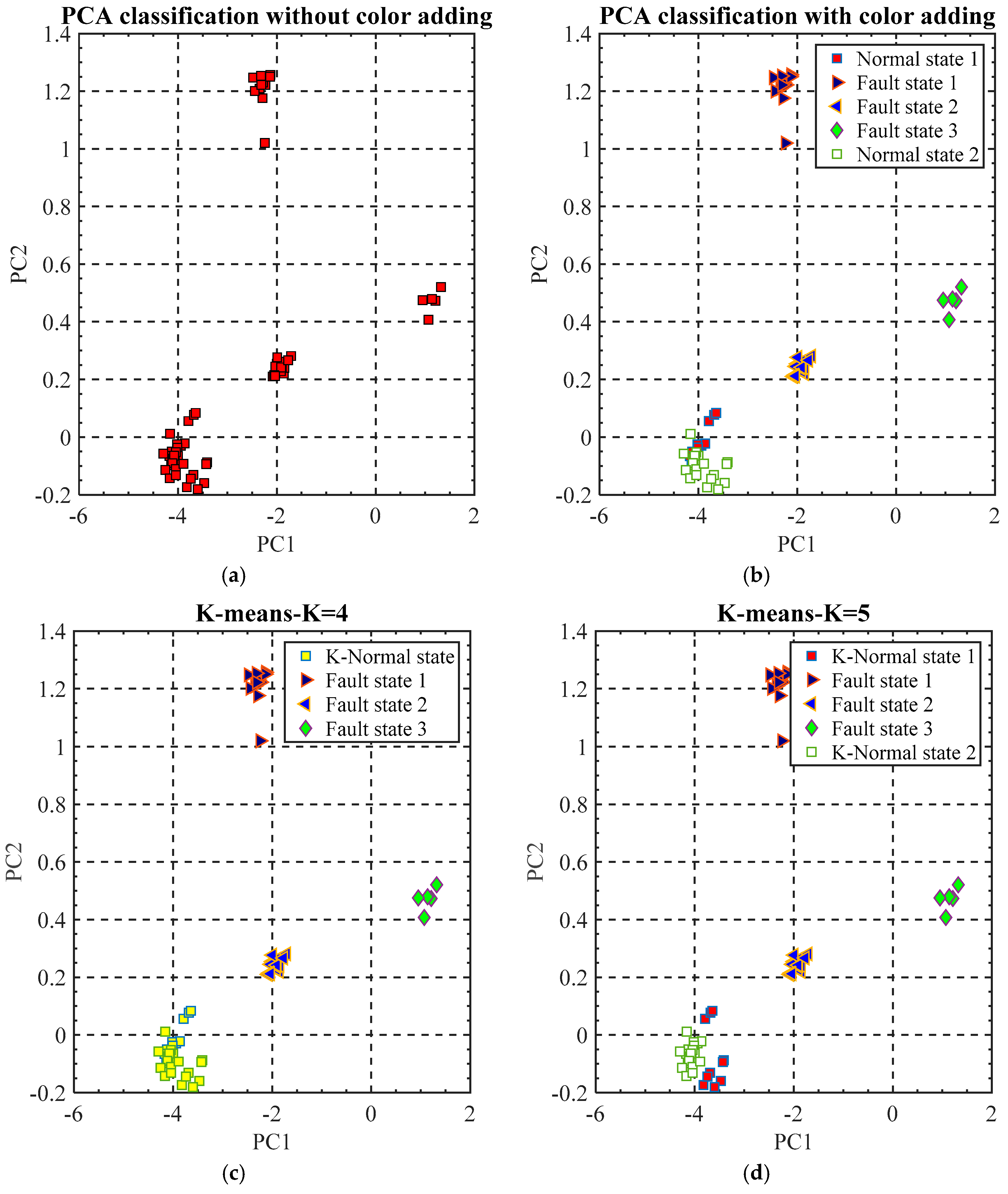
As mentioned, VEs are measured from the machine tool with five states: normal state 1, fault states 1, 2, and 3, and another normal state 2. The five different states could be roughly classified by PCs when they are projected into 2D space (
Figure 10a). The PCA classification results could also be used as a reference for the verification of the cluster number K. For the propose of comparison for the K-means results, different colors have been manually added to the components of the PCA classification results according to the VE testing sequence (
Figure 10b). By this operation, the PCA classification results can clearly reflect the machine tool accuracy states classified by the machine tool user.
K-means classification results are generated automatically without manual supervision (
Figure 10c,d). The K-means classification results reveal that the VE data belonging to the same machine tool state can be classified into one single cluster. The accuracy of the K-means is calculated as the Equation (9) where m is the number of VE samples of each state,
and
stands for the manual label and the K-means cluster label, respectively.
is a function that equals to 1 when
=, if not, it is equal to 0.
For the machine tool fault states 1, 2, and 3 can be perfectly categorized by K-means with K = 4 and K = 5. The classification results match the PCA labelled data (
Figure 10b). For the machine tool normal states 1 and 2, they can be classified into one cluster by K-means when K = 4 (
Figure 10c). Compared with the labelled data shown in (
Figure 10b), normal state 1 and state 2 have been mixed together in one cluster. This indicates that normal state 1 and normal state 2 are very similar when compared with the fault states. When K = 5 (
Figure 10d), K-means could classify the normal state 1 and normal state 2 roughly although some VEs features have been “wrongly” classified. Nine points in the normal state 1 have been classified into normal state 2 and sixteen points in the normal state 2 have been classified into normal state 1. This classification result reveals that for the VE data measured from each normal state, there are still some differences. This is matched with the change tendency of the first PC (
Figure 7). In addition, it can also be explained by the fact that the acquired VE data are measured from machine tool in cold states. This can affect the actual measured VE data and let them perform small changes.
Table 2 reveals the accuracy of K-means with different K value. For the fault states, they could be perfectly recognized from the normal states. As for the normal states 1 and 2, VEs measured in each state are closing but with small differences, so they could be “wrongly” classified. However, this can add a new understanding for the VE measured in the two normal states.
5.3. Discussion
Using the PCA method, the VE features could be extracted and classified by the K-means method. The two methods together can explain the acquired VE data and recognize the machine tool accuracy states. PCA can subtract two principal components from the original VE features. The physical significance of the two principal components has not been investigated because the original VE data are acquired from 29 positions in the machine tool working space with B and C axis in different angular positions. However, there is not specific position requirement on the linear and rotary axis setup when using the SAMBA modelling. Therefore, axis position contributes to VE with the same importance. Meanwhile, the recognition results are more related to the proposed method based on PCA and K-means than the physical meaning of each component.
The proposed VE data processing plan has the following advantages. Firstly, machine tool accuracy states are monitored without considering the sensitivity of VE measurement positions on the faults, in addition, the fault states can be recognized from the normal state of the machine tool. Secondly, it can reveal the differences of the VE measured from the machine tool with similar normal states and provide a visible machine tool accuracy state plot to the machine tool user. Lastly, the features subtracted from PCA shown in the 2D figure could also be used as a reference for K value selection (
Figure 10a). By visual inspection, the K value could be selected as 4 which is matched with the K value selected by the elbow and silhouette methods.
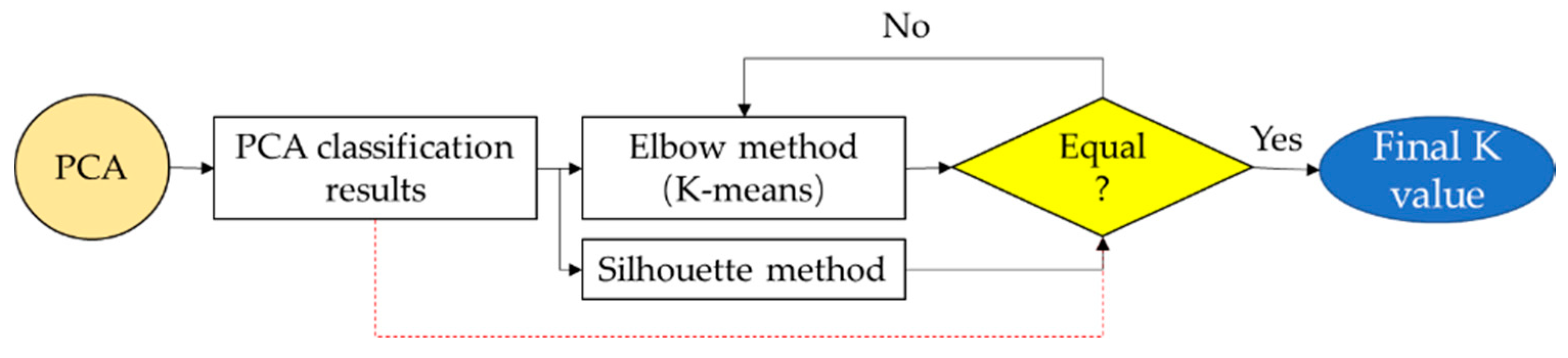
However, some factors can limit the performance of the VE monitoring plan based on PCA and K-means. For the PCA method, the accumulation of VE data is needed before the implementation of PCA. The VE data size is related to the total SAMBA measurement circles (i) and the VE measurement positions (j) in one SAMBA measurement. Where j is fixed, a large amount of VE measurement circles are needed (for example, at least two times of j value). This needs to be verified in the future because no literature reveals the necessary VE data size in PCA application.
For K-means, an exact K value can directly affect the classification results of VE data. To improve the accuracy of K value selection, three K value selection methods are included in the following plan (
Figure 11). PCA method is firstly used for the rough classification of VE data. After that, the VE features will be processed with K-means to find the possible K value by considering the elbow points of
SSE value. Meanwhile, the silhouette value is also calculated for K value verification. In the next step, the cluster number by PCA classification and the K selected by elbow and silhouette method will be compared. When they are matched together, we can get the final K value.
6. Conclusions
This paper explores the use of principal component analysis (PCA) to extract the features of volumetric error vectors (VE) and the use of K-means to classify the machine tool states. The VE data containing two normal states (normal states before and after fault states) and three fault states (C axis encoder fault, uncalibrated C axis encoder fault, and pallet location fault) are processed by PCA and K-means. The testing results reveal that the two proposed methods are effective in their applications. For the PCA method, it can not only subtract the VE feature containing 92.1% of the original VE data but also can reduce the VE data dimension from 67 × 29 to 67 × 2. K-means can automatically classify the VE feature data and successfully recognize the three faults from the machine tool normal states. In addition, the differences of the VE measured in each normal state can also be revealed. Therefore, the two methods could be combined as a new tool for machine tool accuracy state recognition.
However, the question that how to use the classified results to automatically recognize the newly-acquired VE data state still needs to be answered. Therefore, the future work is to develop an online machine tool accuracy state monitoring system using the labelled data and the plan based on PCA and K-means.


