Discrete Element Simulation of Orthogonal Machining of Soda-Lime Glass

Abstract

Transparent, brittle materials, like glass, are used in various applications due to their advantages of mechanical and optical properties. However, their hard and brittle nature causes significant challenges to researchers when they design and test a new machining process. In order to optimize this time-consuming process, discrete element method (DEM) is applied to simulate the cutting process of soda-lime glass in this study. The first step is to create a synthetic material that behaves like soda-lime glass. Then, the macroproperties are calibrated by adjusting the microparameters of the DEM model to match the mechanical properties of the real soda-lime glass. Finally, orthogonal machining simulations are conducted and model validation are conducted by comparing the predicted cutting forces with those from the orthogonal cutting experiments.

1. Introduction

Glass materials are widely used in aerospace, art, cookware and pharmaceutics due to their superior properties such as high strength, hardness, wear resistance, large optical transmission range, and biocompatibility [1]. In modern architecture and civil engineering applications, glass composite, such as laminated glass and glass-fiber-reinforced-polymer, are playing important roles [2,3]. However, due to their high hardness and extreme brittleness, these materials are generally difficult to machine [4]. Glass is classified into several types depending on chemical composition. Soda lime glass is one of these types which is prepared by melting and mixing of silica with alumina, dolomite, lime, and soda at a temperature of up to 1675 °C. The soda lime glass material is used for a wide range of products, such as mirrors, photo masks, data storage disks, microscopic slides, touch screen filters, printed circuit substrates, photographic plates, optical windows, and microfluidic devices [5]. There are several machining processes used to machine soda lime glass including electrochemical discharge machining, precision milling, microwave drilling, precision lathe machining, abrasive jet machining, micro-grinding, and laser machining. Each of them has its unique advantages and disadvantages. Electrochemical discharge machining can achieve high geometrical accuracy and a high machining rate, but micro-cracks and thermal damage are noted on machined surfaces [6]. In a precision machining process, the feed rate significantly affects the cutting forces and surface finish. It is also observed that the higher critical uncut chip thickness at higher cutting speed affect the selection of the feed rate [7]. Drilling of micro-holes can be achieved with microwave drilling. However, high heat is generated due to microwave energy. This caused cracking and deformation defects due to melting in the drilling zone [8]. One example of precision lathe machining is to use an ultra-precision lathe with a single crystal diamond tool. With this machining method, surface roughness is highly dependent on tool wear, which is caused by diffusion, mechanical friction, thermo-chemical action, and abrasive wear [9]. Due to a lack of heat affected zones, the depth of damage to the surface by abrasive jet machining is very little. However, the material removal rate is too low. For example, the typical material removal rate for cutting glass using abrasive jet machining is 16.4 mm³/min [10]. Although a critical depth of 2 to 5 nm and surface roughness of 78 to 980 nm are achieved by a micro-grinding process on soda lime glass material [11,12], the low material removal rate limits the possibility of adopting micro grinding in mass production. Therefore, a hybrid machining methodology, which combines laser micromachining and mechanical machining, is introduced to reduce the cutting force, subsurface damage, and tool wear [1]. Hybrid machining, which combines different machining actions or phases, is able to improve the machining performance. It can take the combined advantages and avoid or reduce some adverse effects the constituent processes produce when they are individually applied [10]. However, due to the high brittleness of glass, the process of random crack initiation and propagation is difficult to study through theoretical analysis and experimental observation. Hence, numerical methods have been used more and more to simulate glass behavior under dynamic loading in recent years [2].

The finite element method (FEM) and extended finite element method (XFEM) have been widely used for numerical simulation of glass cracking and progressive damage in structural and civil engineering applications. For example, in order to optimize the pedestrian protection design for laminated windshields and reduce the severity of head injuries resulting from pedestrian-vehicle crashes, the headform impact response for the laminated windshield is simulated by FEM [13]. With the help of XFEM simulation, researchers are also able to perform a mechanical delamination analysis of the three-dimensional laminated glass model [14]. In addition, FEM has been used in simulating cutting processes in the past few decades, especially in terms of different material properties and cutting conditions on material separation, cutting force, chip formation and heat generation [15]. However, when element distortion becomes large or nodes separate, the failure grids will be deleted and taken out of the cutting zone. It also cannot express the cracks randomly and intuitively because the separation line is usually predefined. Thus, simulating the initiation of cracks in the cutting process is not suitable for FEM. When cracks initiate during machining, the material model for the workpiece would be essentially changed from continuous to discontinuous medium. Discrete element method (DEM) which was introduced by Cundall perfectly solved this type of problems [16]. Due to its meshless feature, large bulks can be separated into small units and it is convenient to deal with large deformation and fracture in cutting processes. Moreover, since the DEM model can describe non-linear behavior, it has great advantages to model the microstructures of brittle materials and handle the complex particle contact physical process with coupled shear and bulk deformation effects. In recent years, DEM has been widely used for simulating cutting processes of brittle materials, such as rock, ceramics, and carbon fiber-reinforced polymer [17,18,19]. In addition to these approaches, a hybrid numerical method is used lately to model the fracture of brittle materials with specific reference to glass [20], in which FEM and DEM are combined satisfactorily in the simulation of a glass beam subjected to a low-velocity hard body impact.

In this paper, the orthogonal cutting process of soda-lime glass is simulated with a DEM model. The purpose is to find out how the DEM model can accurately simulate the cutting process at different cutting conditions. The first step is to create a synthetic material that behaves like soda-lime glass. Then the macro-properties are calibrated by adjusting the micro-parameters of the DEM model to match the mechanical properties of the real soda-lime glass. Finally, orthogonal machining simulations are conducted and model validation are conducted by comparing the predicted cutting forces with those from the orthogonal cutting experiments. Through this study, the DEM simulation of the orthogonal cutting process of soda-lime glass is identified and validated.

2. DEM Model of Soda-Lime Glass

Particle flow code in two dimensions (PFC2D) [21] is used to create a synthetic material that behaves like soda-lime glass. PFC2D is a commercial DEM simulation software which is widely used for different engineering applications. PFC2D models the interactions and movements of circular particles by distinct element method, which allows finite displacements and rotations of discrete bodies, including complete detachment, and recognizes new contacts automatically as the calculation progresses. PFC2D can model a solid by bonding every particle to its neighbors and compacting the particles within four walls. The resulting assembly is able to not only possess elastic properties, but also maintains plastic properties which can generate fractures when bonds between these particles break. Although the standard bonded-particle model (BPM) has been successfully applied to solve a wide range of problems, there are still some intrinsic problems that cannot be avoided using the standard BPM, such as an unrealistically low unconfined compressive strength to tensile strength (UCS/UTS) ratio, an excessively low internal friction angle, and a linear envelope [22]. In order to avoid those problems in the simulating process, it is decided to apply the flat-joint model to model soda-lime glass.

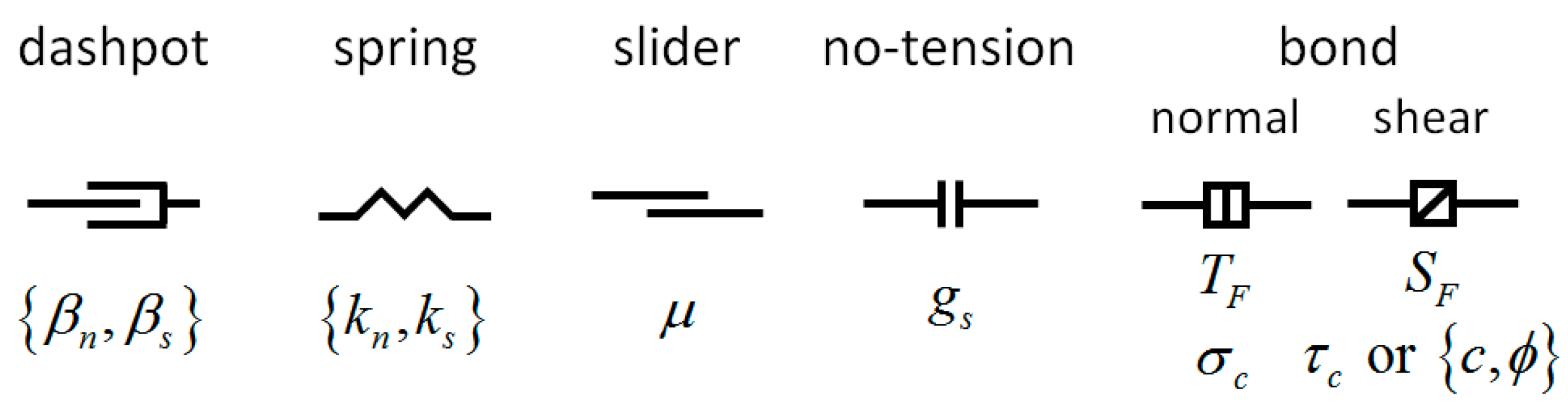
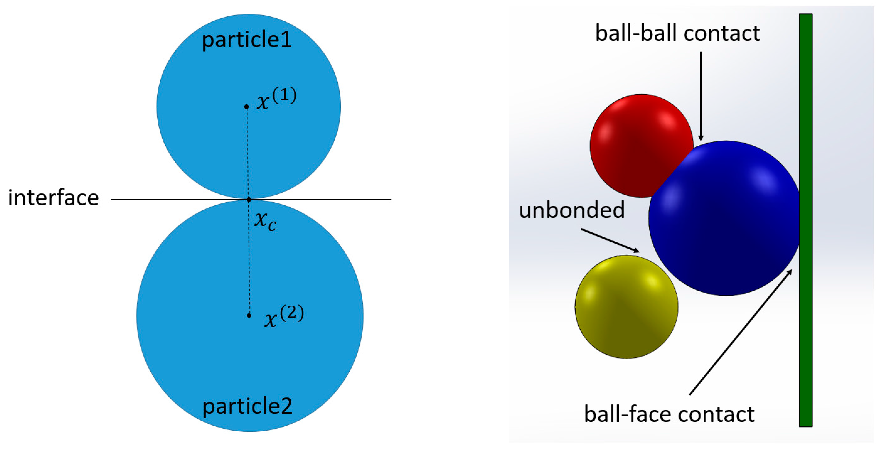
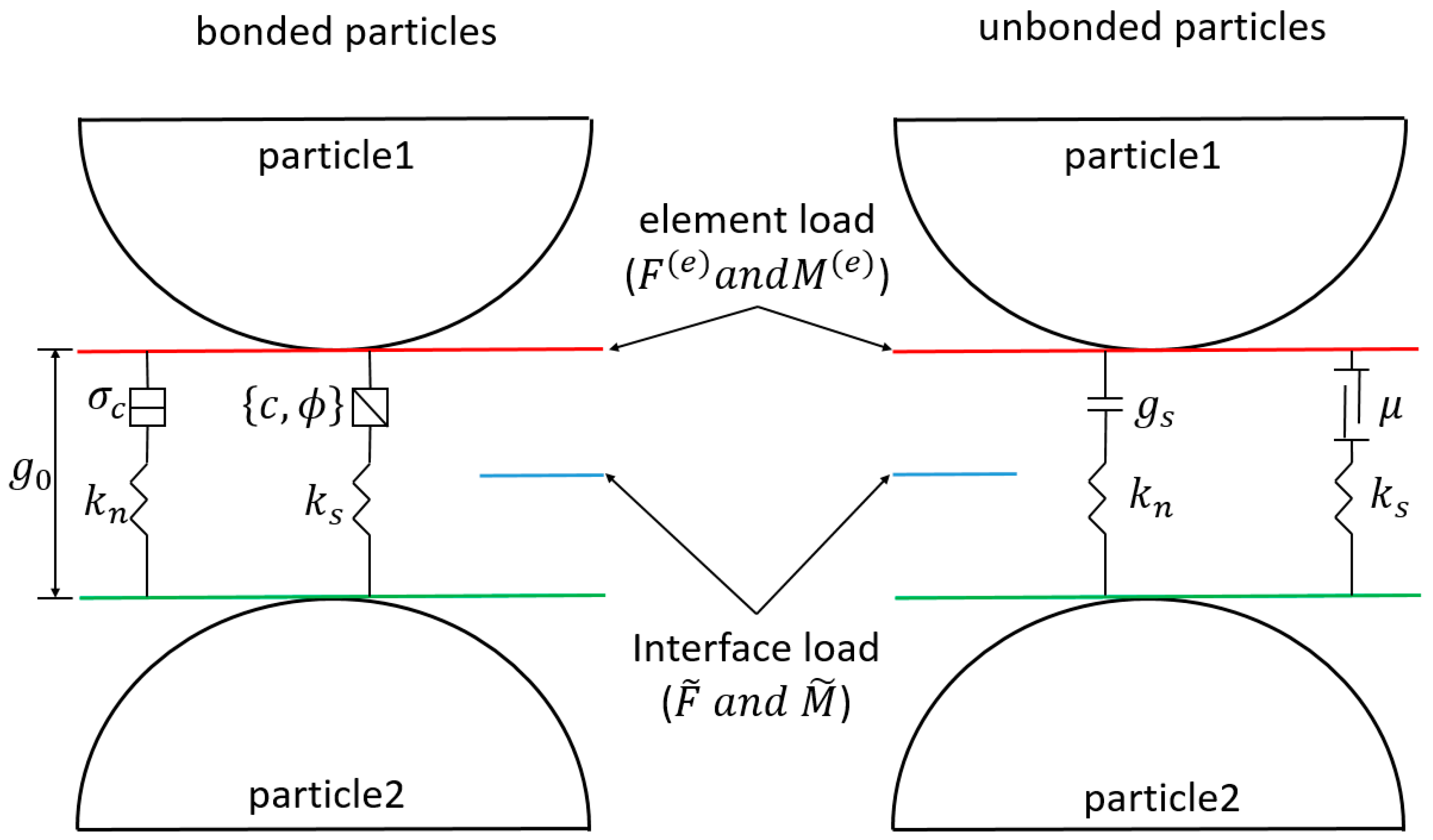
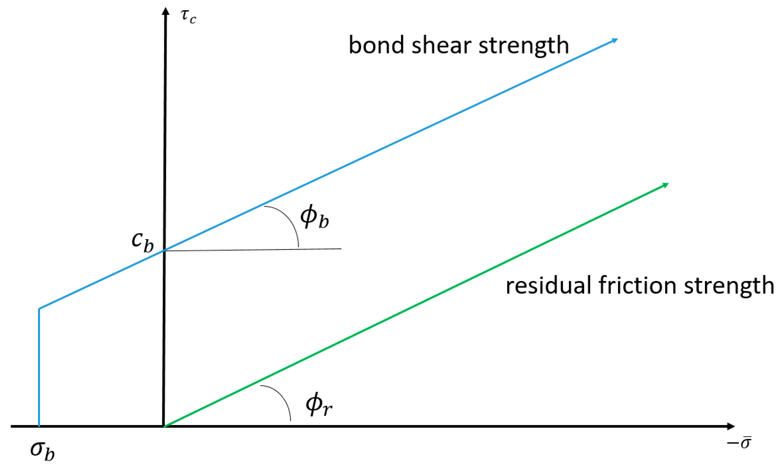
2.1. Fundamentals of Flat-Joint Model

Flat-joint is an interface of ball-ball or ball-face contact (Figure 1) which can be deformable, partially damaged, and breakable. The breakage of each bonded element contributes partial damage to the interface and is denoted as a crack. The flat-joint model provides the macroscopic behavior of a finite-size, linear elastic, and either bonded or frictional interfaces that may sustain partial damage. A bonded element has a linear elastic behavior until the strength limit is exceeded and bond breaks, making the element unbonded. An unbonded element has linear elastic and frictional behavior with slip accommodated by imposing a Coulomb limit on the shear force.

After a flat-joint contact is installed, the force and moment in each element are initialized to zero. Then they will be updates by generalized force-displacement law which demonstrate internal force to the relative motion at the contact. Each element carries a force and moment (F^(e) and M^(e)) that act at the element centroid (Figure 2), and the formulation is expressed in terms of a set of internal rheological parameters (Figure 3).

The element forces and moments produce a statically equivalent force and moment at the center of the interface by:

$$\tilde{F}={\displaystyle \sum _{\forall e}}{F}^{\left(e\right)},\tilde{M}={\displaystyle \sum _{\forall e}}\left\{\left(r^{\left(e\right)}\times F^{\left(e\right)}\right)+M^{\left(e\right)}\right\}$$

(1)

where r^(e) = x^(e) − x_c is the relative position, x^(e) is the centroid location of element (e) and x_c is the center of the interface.

The element normal stress and shear stress are given by:

$${{\sigma }_{max}}^{\left(e\right)}=\frac{{F_n}^{\left(e\right)}}{A^{\left(e\right)}},{{\tau }_{max}}^{\left(e\right)}=\frac{\Vert {F_s}^{\left(e\right)}\Vert }{A^{\left(e\right)}}$$

(2)

where F_n and F_s are the normal and shear forces acting at the element, A is the area of the element.

There are two main types of elements for a flat-joint contact, which are bonded elements and unbonded elements. The bonded element’s strength envelope is as follows (Figure 4).

${\sigma }_b$ is the tensile strength and the elements will break with a tensile crack when ${\sigma }_{max}>{\sigma }_b$. The shear strength is ${\tau }_c$ which follows the Coulomb criterion given by:

$${\tau }_c=c_b-\overline{\sigma }\tan {\varphi }_b$$

(3)

where $c_b$ is the bond cohesion, $\overline{\sigma }$ is the normal stress, and ${\varphi }_b$ is the local friction angle. The shear stress will lock to ${\tau }_{max}$ when ${\tau }_{max}<{\tau }_c$, or the bond will break in shear and the residual friction takes effects:

$${\tau }_r=-\overline{\sigma }\tan {\varphi }_r$$

(4)

where ${\tau }_r$ is the residual friction strength and ${\varphi }_r={tan}^{-1}\left(\mu \right)$ is the residual friction angle. This type of element can be broken with a tensile or shear crack.

Additionally, the unbonded elements follow such a force-displacement law. The normal stress is given by:

$$\overline{\sigma }=\{\begin{array}{cc}0,\hfill & \hfill \mathrm{unbonded}\mathrm{and}\overline{g}\ge 0\\ -k_n\overline{g},\hfill & \hfill \mathrm{otherwise}\end{array}$$

(5)

where k_n is the normal stiffness and $\overline{g}$ is the interface gap. The shear strength follows the Coulomb sliding criterion:

$${\tau }_r=\{\begin{array}{ccccc}-\overline{\sigma }\tan {\varphi }_r,& & & & \overline{\sigma }<0\\ 0,& & & & \overline{\sigma }=0\end{array}$$

(6)

where ${\varphi }_r$ is the residual friction angle. When the shear stress ${\tau }_{max}<{\tau }_r$, it remains as ${\tau }_{max}$, or the shear stress will change and enforces sliding at the interface. Within this type of element, there is no tensile or shear crack.

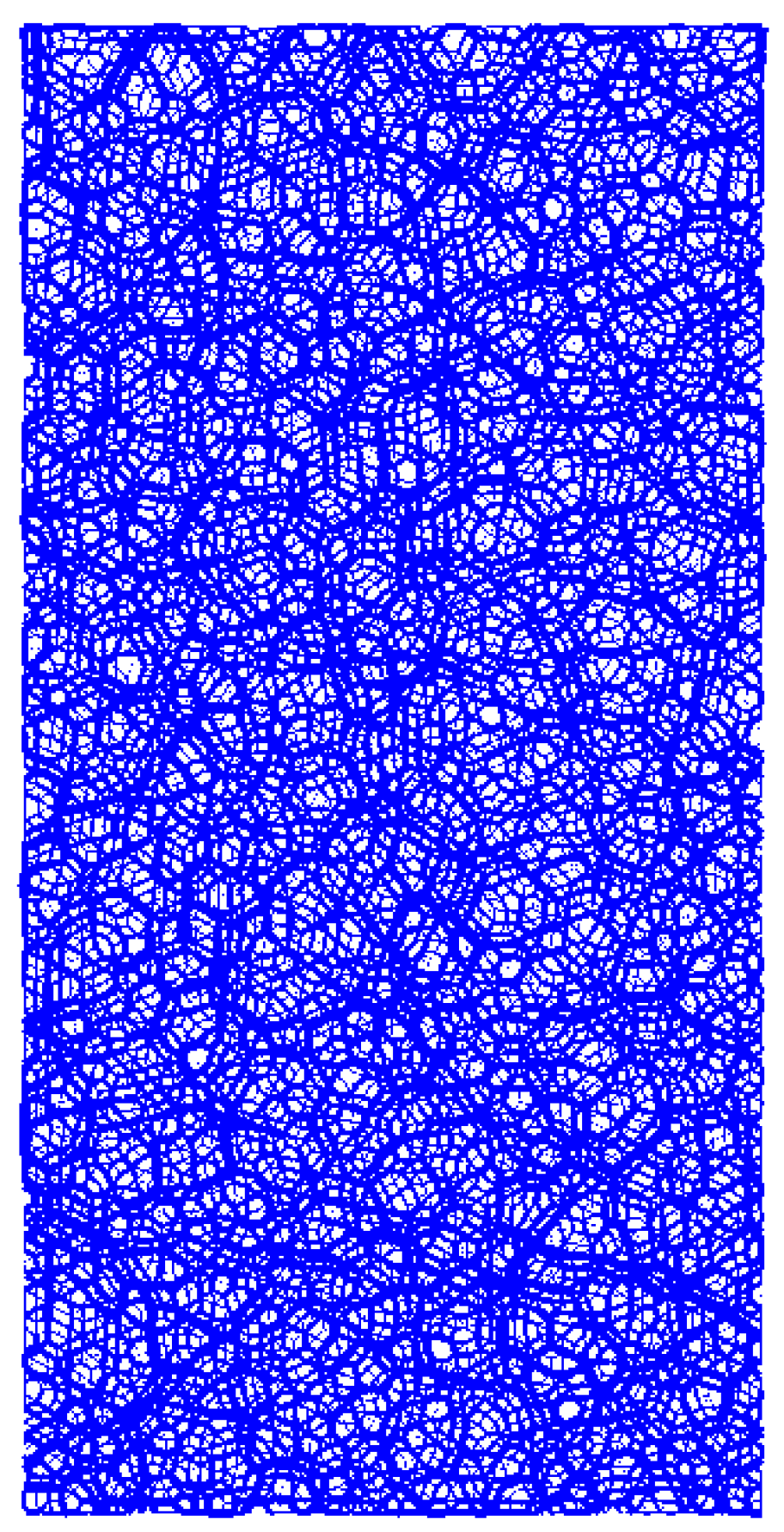
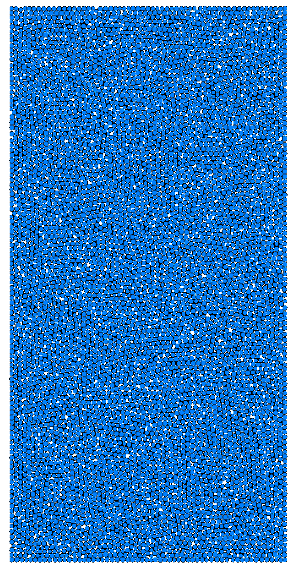
2.2. Creation of the Bonded Particle Specimen

The first, and most crucial, step of a successful numerical simulation is to create the specimen that behaves like the real material. There are three general steps to generate the specimen in PFC2D: (1) creating a dense particle assembly; (2) installing flat-joint bonds at contacts; and (3) removing confinement for the specimen. The specimen produced by this procedure is a well-connected particle assembly with low locked-in forces. There are two sets of parameters which need to be defined when creating a synthetic specimen (

Table 1. Macro- and micro-parameters of the synthetic specimen.

Macro-Parameters	Description	Value	Micro-Parameters	Description	Value
ρ	Ball density (kg/m3)	2.4 × 103	$E_c$	Ball-ball contact modulus (Pa)	107.0 × 109
H	Sample height (m)	2.0 × 10−3	$k_n/k_s$	Ball stiffness ratio	3.1 × 10
W	Sample width (m)	1.0 × 10−3	${\overline{E}}_c$	Flat-joint bond modulus (Pa)	107.0 × 109
Rmin	Minimum ball radius (m)	1.5 × 10−5	${\overline{k}}_n/{\overline{k}}_s$	Flat-joint bond stiffness ratio	3.1 × 10
Rmax	Maximum ball radius (m)	2.0 × 10−5	$\mu$	Ball friction coefficient	0.577
			${\overline{\sigma }}_c$	Flat-joint normal strength (Pa)	200.0 × 106
			${\overline{\tau }}_c$	Flat-joint shear strength (Pa)	113.0 × 106
			$\varphi$	Friction angle (degree)	25.0 × 10

). One includes the geometric and physical parameters, which are the specimen height, specimen width, particle size, and particle density. The other contains constitutive parameters to define the micro properties of the particles and their contact and bond, which contain the particle contact stiffness, particle stiffness ratio, particle friction coefficient, particle damping coefficient, bond shear strength, bond normal strength, and friction angle.

A synthetic specimen is created following the procedure and considerations mentioned above, as shown in Figure 5. The micro-parameters needed for the specimen generation are estimated values at this point and will be adjusted to match the actual material properties in the next section. The specimen is 2 mm in height and 1 mm in width. It contains 7406 circular disks of unit thickness and the radii of the disks range from 15 to 20 μm. The particle density is set to be 2400 kg m⁻³ according to soda-lime glass properties [23]. The network shown in Figure 6 indicates the flat-joint bonds, which are the straight lines connecting the particles together.

3. Calibration of the DEM Model (Mechanical Properties)

It is known that the macro-properties of the DEM model are directly related to the micro-parameters of the flat-joint contact model. However, there is no definite relationship between macro-properties of the sample and the micro-parameters of the flat-joint model. Thus, a series of tests need to be conducted to calibrate the model and make sure that the simulation model has the equivalent properties with those of soda-lime glass. The macro-properties to be matched are elastic modulus (E), Poisson’s ratio (ν), ultimate tensile strength (σ_t), and compressive strength (σ_c).

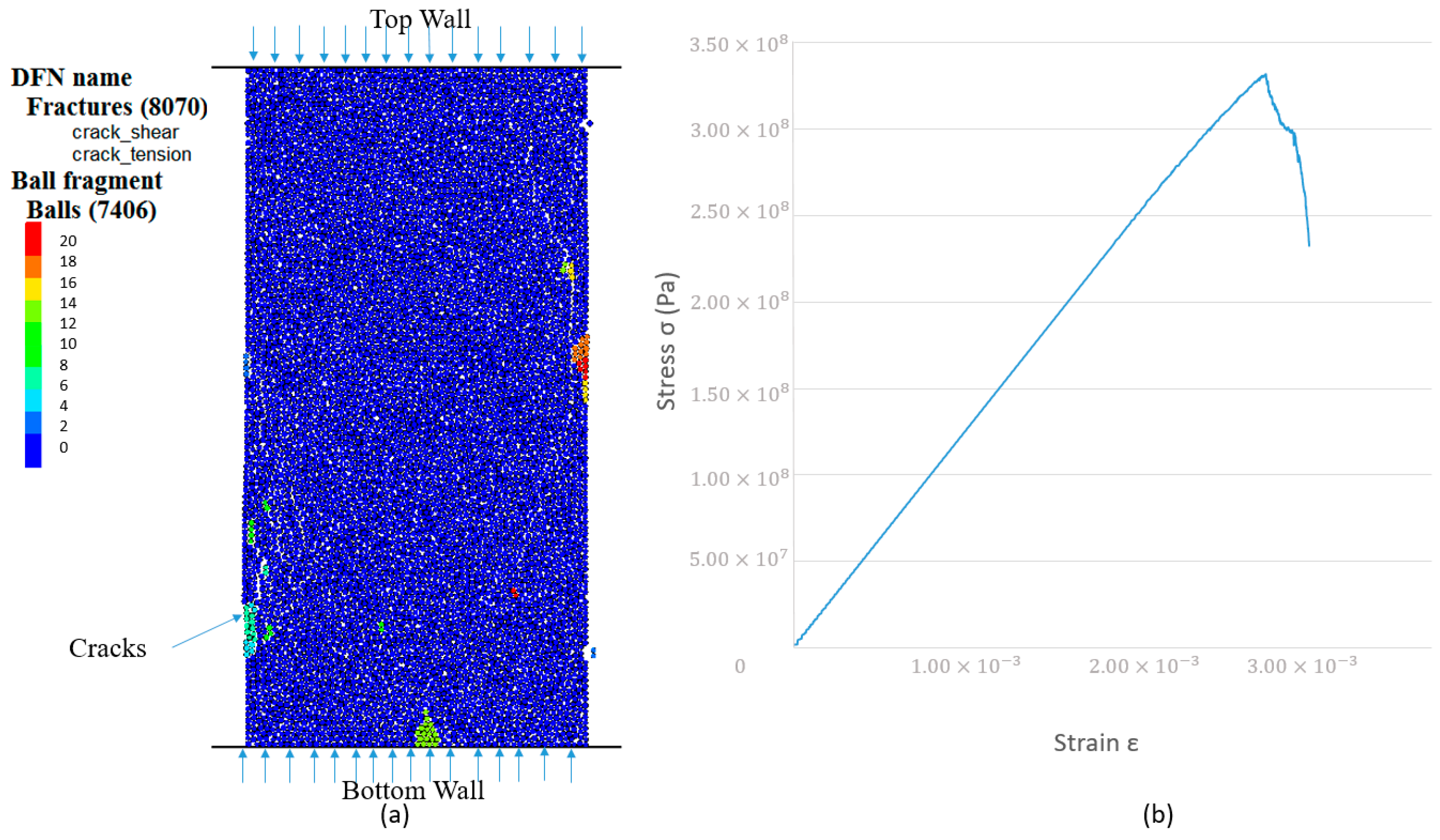
3.1. Uniaxial Tensile Test

The same specimen created in the previous section is used for the uniaxial tensile test. A row of particles at the top and bottom of the sample are identified as “grips”. As shown in Figure 7a, the top grip is moved upward and the bottom grip is moved downward with the same speed of 0.02 mm/min to apply tensile loading. The model is loaded until the axial stress drops to 70% of the peak stress. The fracturing is tracked by monitoring the broken bonds and the cracks are plotted during the test. The cracks can be generated by both shear and tensile force, which are also shown as green and red lines in Figure 7a. Additionally, there are two important quantities being recorded during the test. One is the stress, which is the average stress in the measurement region of the sample [24]. The other is the strain, which is the ratio of total deformation to the initial height of the sample. Since PFC2D is able to track the positions of each particle during the simulation, the displacement of the particles can be calculated and retrieved by manipulating the FISH functions which is an embedded programming language of PFC2D. As shown in Figure 7b, the stress-strain curve can be plotted. Elastic modulus and tensile strength can be identified through the plot.

3.2. Uniaxial Compressive Test

The same specimen is used for the unconfined compressive test. Instead of “grips”, two rigid walls are created at the top and bottom surface of the sample as shown in Figure 8a. These two walls are considered as rigid supports, which cannot be deformed or broken during the process. During the compressive test, the top wall is moved downward and bottom wall moved upward with the same speed of 0.02 mm/min to apply compressive loading. The model is loaded until the axial stress drops to 70% of the peak stress. With the same method as the uniaxial tensile test, the stress-strain curve can be plotted, as shown in Figure 8b.

Since the strain in transverse direction can be calculated as well, we can determine the Poisson’s ratio, which is the ratio of transverse strain to axial strain. The normal and most straightforward method for measuring Poisson’s ratio is conducting a normal mechanical tensile test [25]. Thus, the Poisson’s ratio is calibrated through the uniaxial tensile test. Through a series of adjustments, the DEM model is calibrated to match the soda-lime glass properties as listed in

Table 2. Comparison of properties between the DEM model and soda-lime glass.

Mechanical Property	Elastic Modulus E (GPa)	Tensile Strength σt (MPa)	Compressive Strength σc (MPa)	Poisson’s Ratio ν
Soda-lime glass	71	41	330	0.23
DEM Model	71.1	42.6	332	0.228

. The next step is to simulate the cutting processes of the specimen.

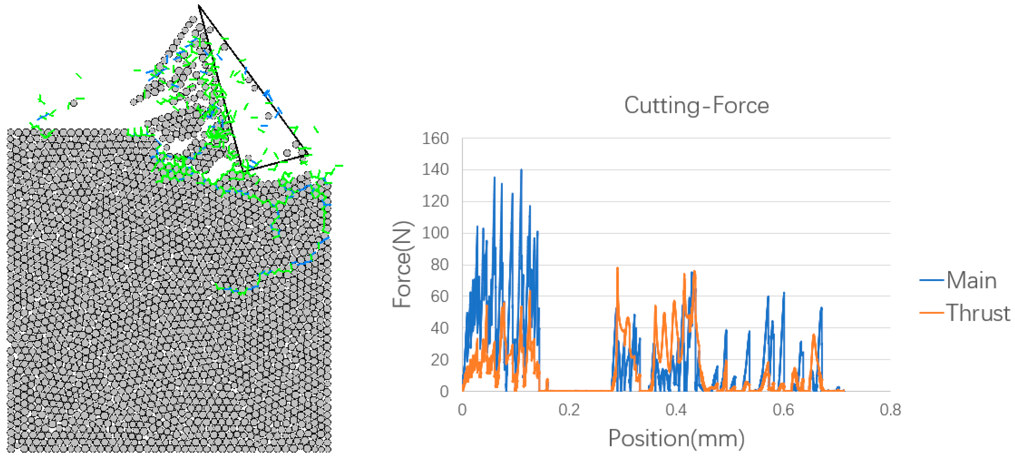
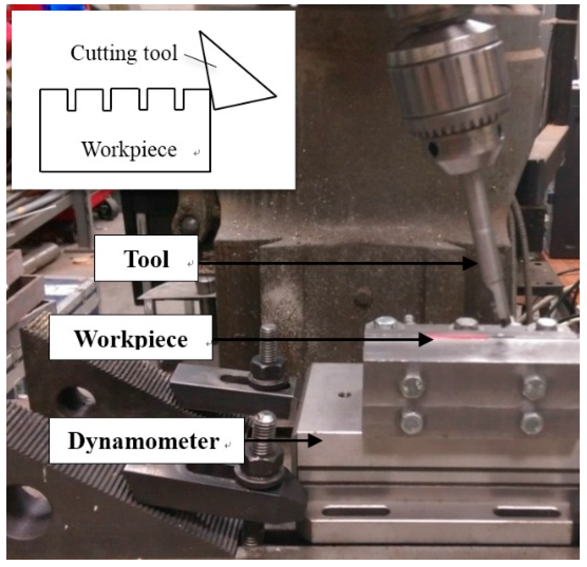
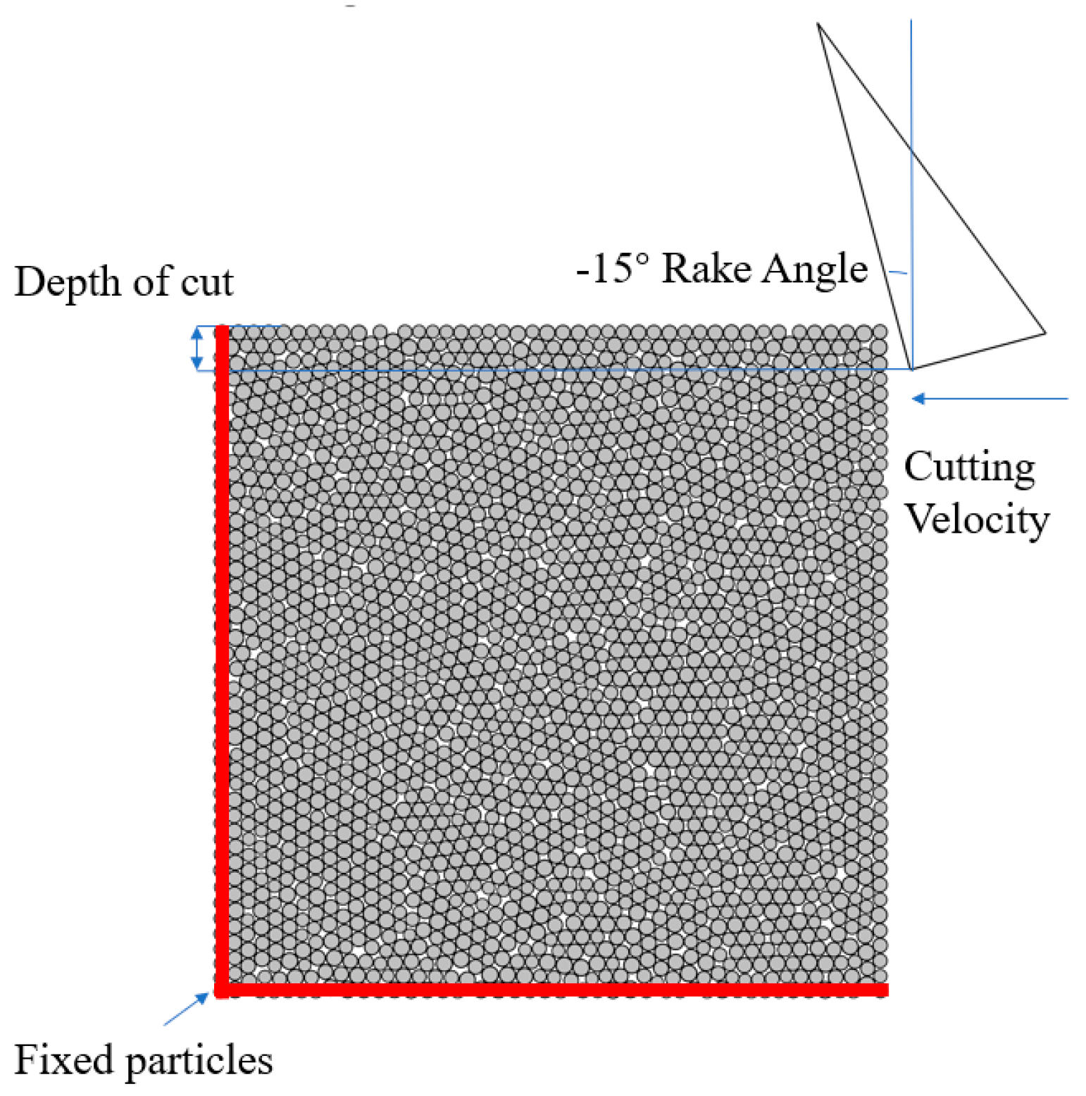
4. Cutting Simulation

The orthogonal cutting with different cutting conditions is simulated and each simulation is repeated three times using specimens generated with different random particle arrangements to reduce the influence of particle arrangement. The cutting conditions are shown in

Table 3. Cutting conditions for the simulation.

Parameter	Description	Value
V (mm/s)	Cutting speed	4.23
t (mm)	Depth of cut	0.1, 0.2
α (degree)	Rake angle	−15
L (mm)	Width of cut	1

. The model geometry and boundary conditions for the cutting simulation are shown in Figure 9. The glass workpiece is 1 mm in length and 1 mm in height, and it contains 2085 particles. The particles on the left side and bottom side of the workpiece are fixed. The cutting tool is modeled as a rigid body using wall elements which has the same rake angle (−15°) and same clearance angle (15°) during the cutting simulation. The depths of cut are 0.1 mm and 0.2 mm with the fixed cutting speed of 4.23 mm/s.

The glass specimens have two different surface conditions. One is laser-treated with grooves on the top surface induced by femtosecond laser micromachining [1]. The groove depths are 0.1 mm and 0.2 mm according to the depth of cut. The groove distance and width are 0.2 mm and 0.06 mm (Figure 10). The other type of specimen is the untreated sample which does not have microgrooves.

Thus, there are a total of four different conditions to simulate for the cutting process: (1) 0.1 mm depth of cut without microgrooves; (2) 0.1 mm depth of cut with microgrooves; (3) 0.2 mm depth of cut without microgrooves; and (4) 0.2 mm depth of cut with microgrooves. The main (horizontal direction) and thrust (vertical direction) cutting forces are recorded during the simulation. Figure 11, Figure 12, Figure 13 and Figure 14 show the results for each cutting condition:

(1)

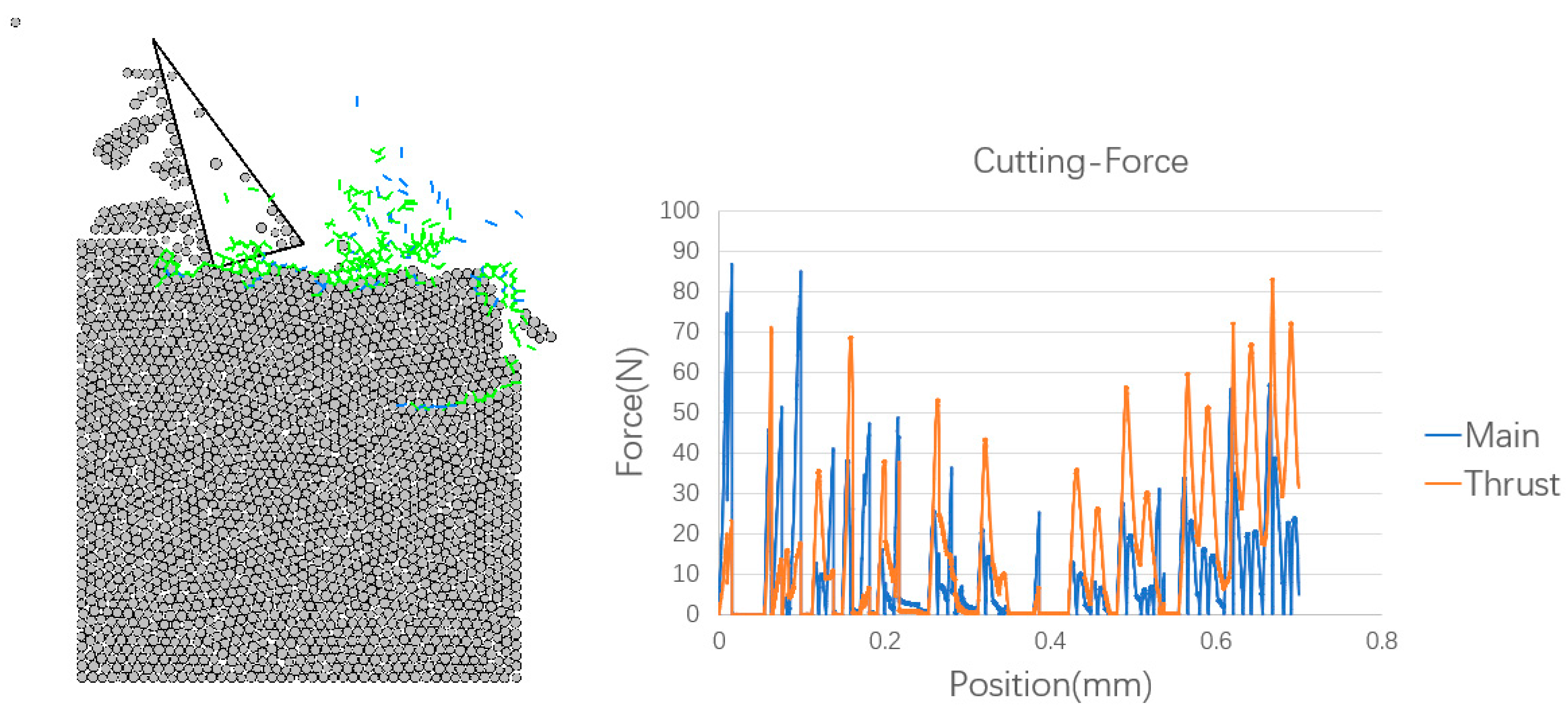
A 0.1 mm depth of cut without microgrooves:

(2)

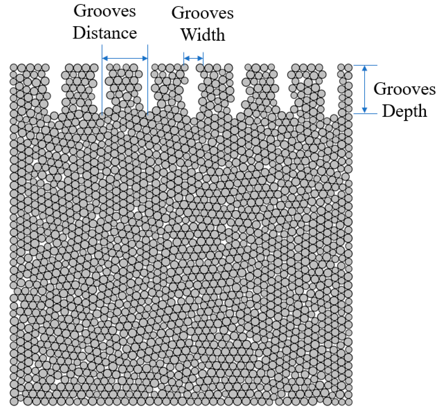
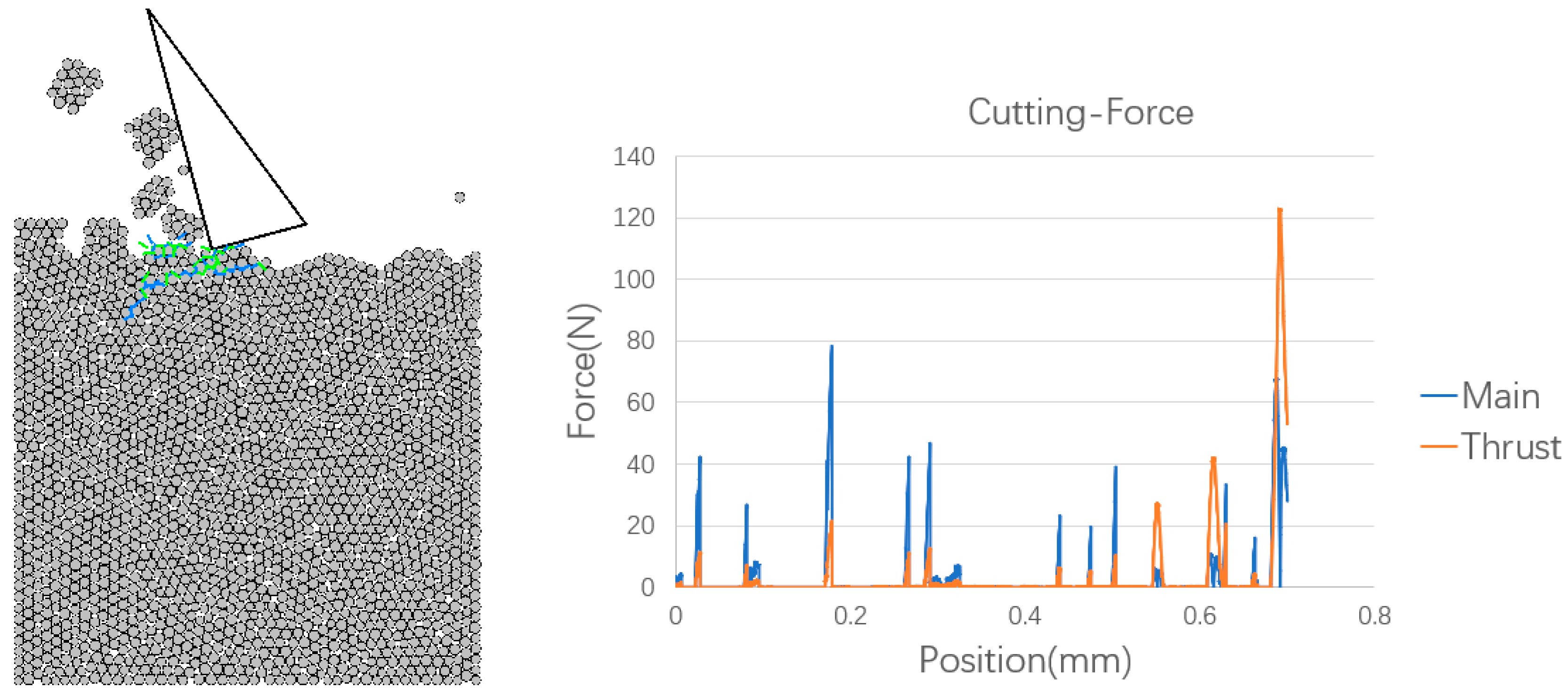
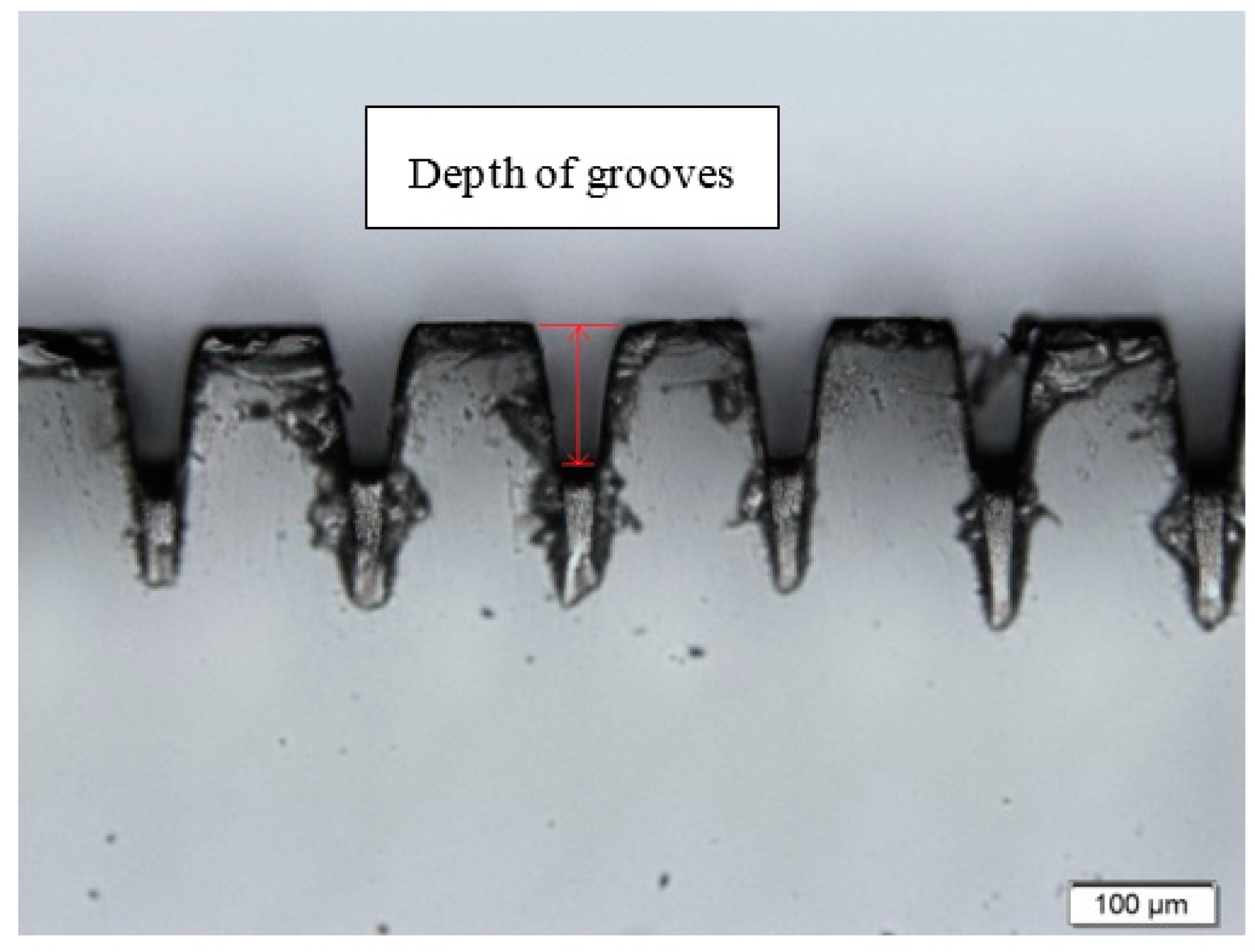
A 0.1 mm depth of cut with microgrooves:

(3)

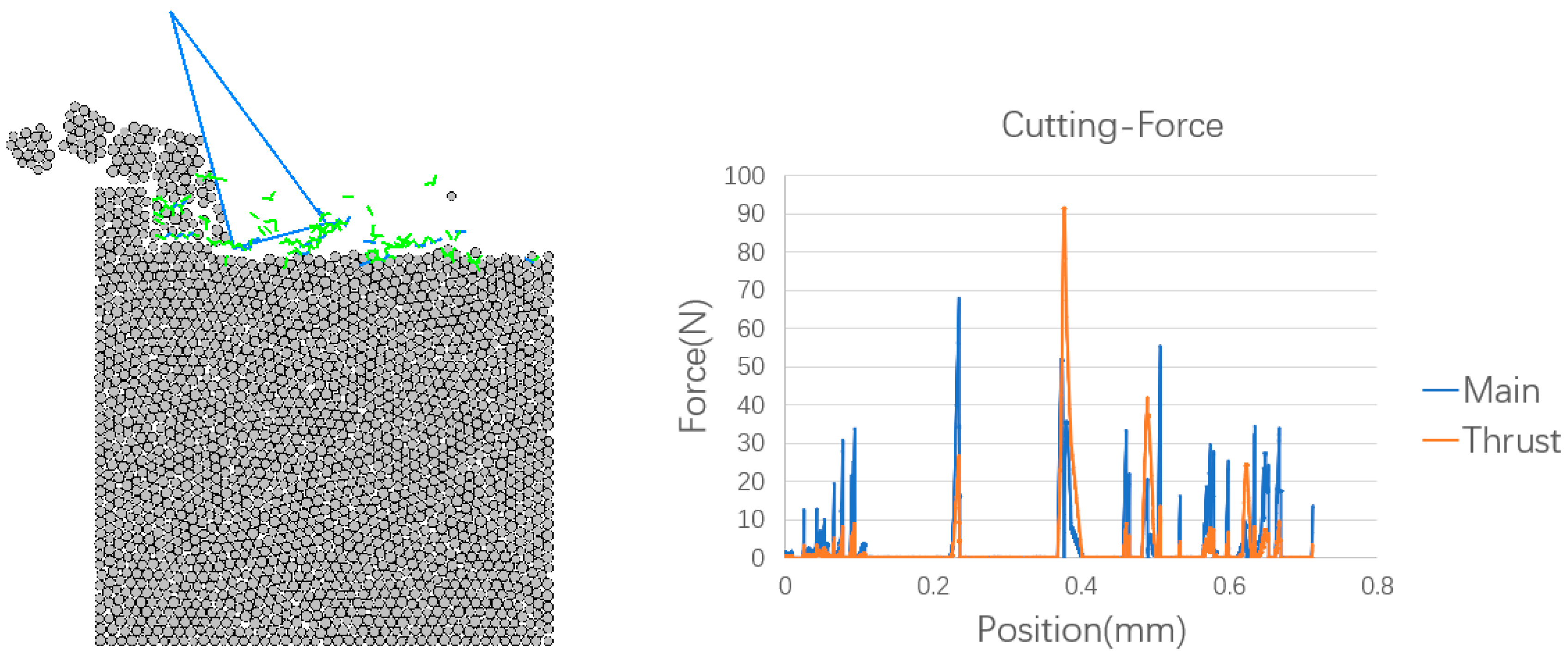
A 0.2 mm depth of cut without microgrooves:

(4)

A 0.2 mm depth of cut with microgrooves:

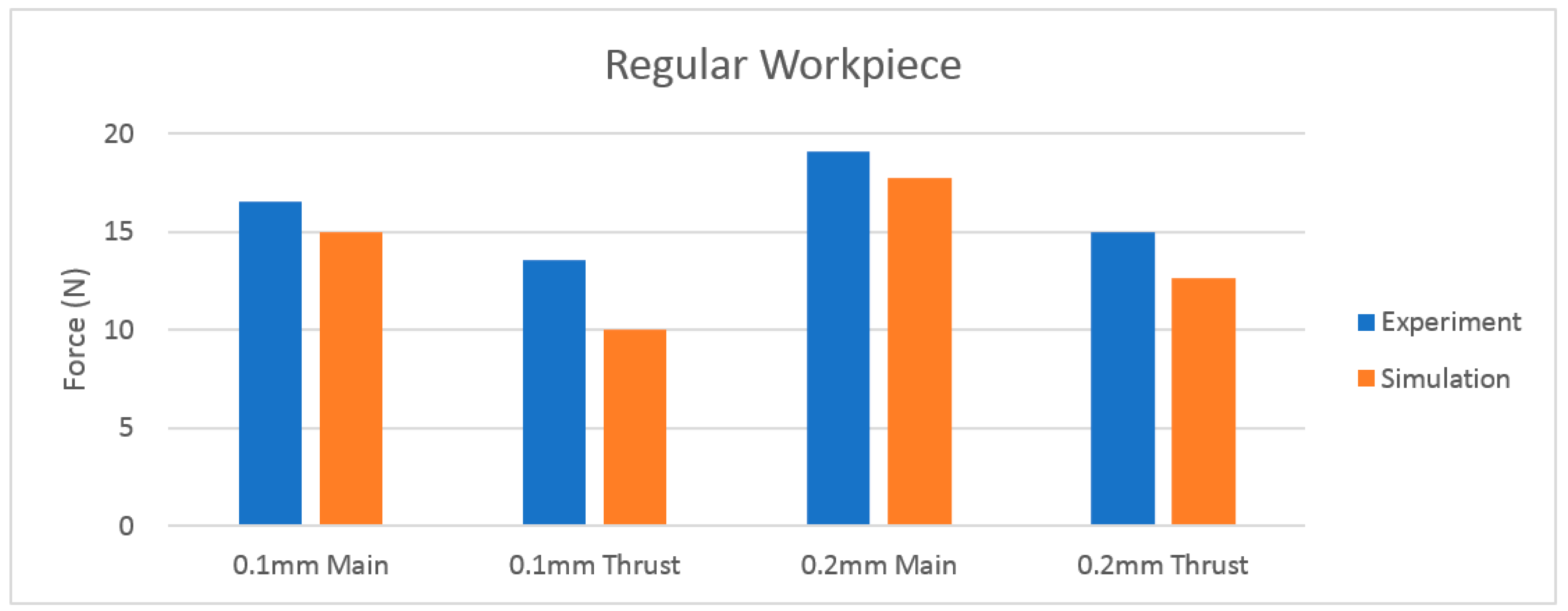
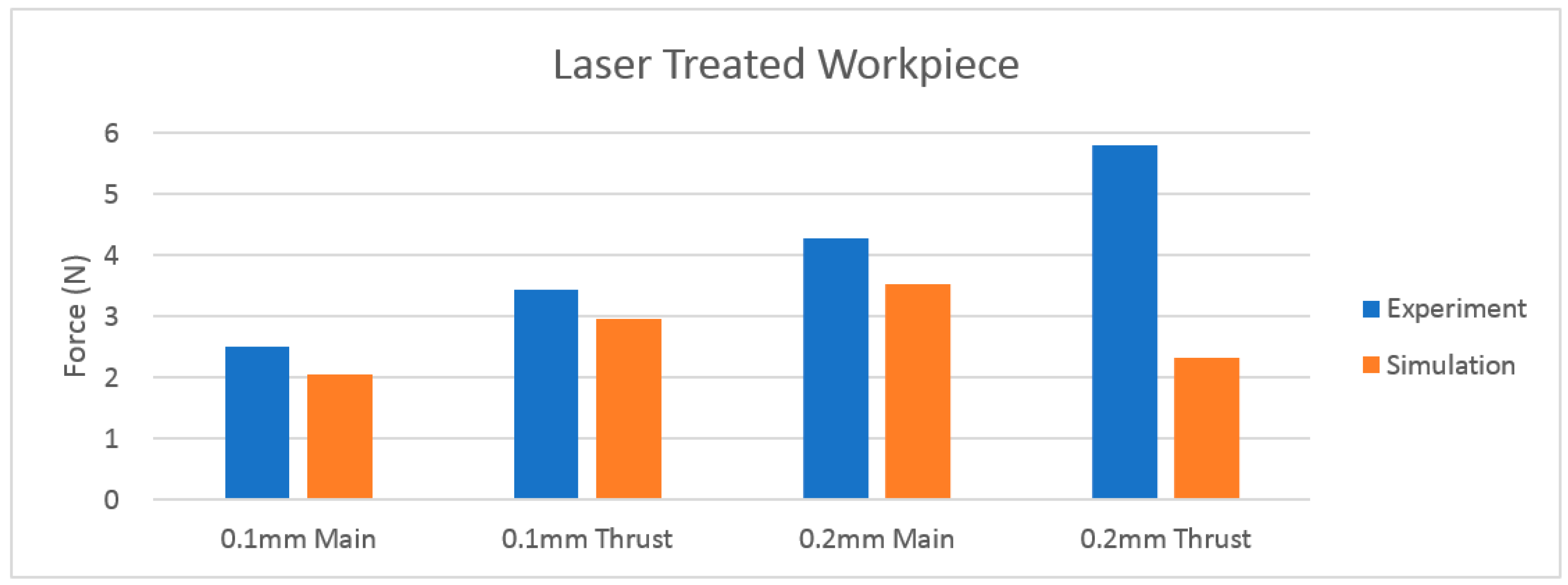
In all the chip formation images, the green, short lines denote broken bonds between the particles which are caused by shear failure; the blue, short lines are also broken bonds, but they are caused by tensile failure. It is obvious that chip formation is due to initiation and propagation of brittle cracks in the material and varied size of chip segments are the evidence for the brittle material removal process. As the depth of cut increases from 0.1 mm (e.g., Figure 11) to 0.2 mm (e.g., Figure 13), chips become larger and subsurface cracks become deeper in general. Additionally, there are distinct differences between the regular and grooved workpieces under the same cutting conditions. First, the broken bonds are less for the grooved workpiece, which is particularly true for the 0.2 mm depth of cut when comparing Figure 13 and Figure 14. Second, the cracks left on the machined part are shorter and shallower for the grooved workpiece. The main benefit of installing microgrooves on the workpiece is reducing the subsurface cracks dramatically. The workpiece is very strong without the microgrooves and needs a large force to initiate a crack. With microgrooves on the surface, the workpiece is significantly weakened. Since cracks initiate mainly at the bottom of the microgrooves, which is the weakest part of the workpiece, less force is needed to initiate a crack and subsurface cracks are almost nonexistent.

The cutting forces in both the horizontal and vertical directions are recorded during the simulation process. It can be seen that numerous force peaks exist for both the regular and grooved workpieces, which are caused by the initiation and propagation of cracks due to bond breakage between particles. This behavior is typical for brittle material removal processes, characterized by random peaks and valleys which correspond to force build-up followed by sudden fracture occurrence. It is found that the force magnitude for the grooved workpiece is much smaller than for the regular one because the grooves reduce the material strength. It is also reasonable that when the depth of cut is reduced, the cutting force is reduced correspondingly. The average forces are listed in

Table 4. Average cutting forces in horizontal and vertical directions.

Depth of Cut (mm)	Replications	Average Cutting Force (N)
		Regular Workpiece		Grooved Workpiece
		Main	Thrust	Main	Thrust
0.1	1	14.15	10.29	1.72	2.84
	2	15.40	9.27	2.82	3.13
	3	15.38	10.38	1.60	2.87
0.2	1	17.45	13.54	3.68	2.98
	2	17.24	12.16	3.14	2.95
	3	18.41	12.19	3.73	1.06

for comparison.

5. Model Validation

In order to validate the simulation model, the orthogonal machining experimental setup is constructed using a vertical Bridgeport milling machine with a cutting tool fixed on the locked vertical spindle column. The soda-lime glass is fixed on the horizontal carriage (Figure 15). The fixture is mounted onto a Kistler three-component dynamometer. A Kistler dual-mode charge amplifier is used to amplify cutting force signals measured by the dynamometer. LabView (National Instruments, Austin, TX, USA) is used to control the computer data acquisition system. The workpiece, fixture, and dynamometer are clamped onto the movable carriage of the Bridgeport milling machine. The horizontal carriage feeds the workpiece on to the stationary tool holder which is mounted in the vertical tool chuck. A 15.875 × 15.875 × 6.35 mm ceramic insert is used as a cutting tool. A special tool holder, tilted to attain a negative 15-degree rake angle is used for the experiment. The cutting conditions are given in

Table 5. Cutting conditions for the experiments.

Parameter	Description	Value
V (mm/s)	Cutting speed	4.23
t (mm)	Depth of cut	0.1, 0.2
α (degree)	Rake angle	−15
L (mm)	Width of cut	25.4

.

The cutting experiments contain four conditions which are exactly the same as in the simulation. For the laser treated samples, the microgrooves are made by laser scanning at the sample surface as shown in Figure 16. The main differences between the treated samples are the groove depths. For the 0.1 mm depth of cut, the groove depth is 0.1 mm. For the 0.2 mm depth of cut, the groove depth is 0.2 mm.

The dynamometer is calibrated before conducting the experiments. Force data is collected at a sampling rate of 200 data points per second.

Table 6. Average cutting forces for each experiment.

Depth of Cut (mm)	Replications	Average Cutting Force (N)
		Regular Workpiece		Laser Treated Workpiece
		Main	Thrust	Main	Thrust
0.1	1	17.8	14.1	2.0	3.1
	2	15.0	12.5	2.9	4.0
	3	16.7	14.0	2.6	3.2
0.2	1	19.9	15.5	4.3	5.6
	2	18.1	14.6	4.6	6.4
	3	19.2	14.8	3.9	5.4

shows the average cutting force recorded during each experiment.

In order to compare the simulation and experimental results for each condition, the average forces for the three replications are taken and plotted in Figure 17 and Figure 18. In general, the experimental forces are 7–26% more than the simulation results. For most of the cases, the difference between the simulation and experimental results are below 20%. Especially for the regular workpiece, the results are more reliable and repeatable because the macro-properties of the EDM model are close to the real condition. However, for the grooved workpiece, the results are not as good as for the regular workpieces. For the 0.2 mm depth of cut of grooved workpieces, the thrust force from the experiment is about 60% larger than the simulation result. A possible reason is that the groove geometry of the model is different from that of the real workpieces. The grooves of the laser-treated sample have an inverted trapezoidal shape, which means the bottom wall of the groove is thicker and stronger. However, for the DEM model, the grooves are made by deleting the particles within certain areas, so that the groove walls are more like rectangular shape, which are weaker at the bottom compared with the trapezoidal-shaped walls for the real workpieces. This effect will become more obvious for the 0.2 mm depth of cut since the wall becomes taller and less force is needed to break the bonds. This argument will be carefully examined in future simulation work.

6. Conclusions

In this paper, the orthogonal cutting of soda-lime glass is simulated with PFC2D base on discrete element method. The results of cutting force, subsurface cracks and chips are studied, and the cutting forces are validated through the orthogonal cutting experiment. The following conclusions are obtained from this study.

• The cause of crack initiation can be identified by the simulation model. There are two types of cracks: one is caused by shear force and the other is caused by tensile force.
• The simulations show that cutting forces can be reduced and subsurface cracks can be eliminated when cutting grooved workpieces.
• The geometries of the simulation model highly affect the result. Compared to the grooved specimen, the simulation result for the regular one is more accurate and repeatable.
• Simulation time is highly dependent on the number of particles for the model and computing capacity. Smaller particle size and larger number of particles can enhance the details of the model. More powerful computing methods are recommended, such as parallel computing and supercomputing to increase the simulation efficiency.

References

1. Shanmugam, N.; Yu, X.; Alkotami, H.; Devin, G.; Lei, S. Machining of Transparent Brittle Material Assisted by Laser-Induced Seed Cracks. In Proceedings of the ASME 2016 11th International Manufacturing Science and Engineering Conference, Blacksburg, VA, USA, 27 June 27–1 July 2016; V001T02A019. American Society of Mechanical Engineers: New York, NY, USA, 2016. [Google Scholar]
2. Larcher, M.; Arrigoni, M.; Bedon, C.; Van Doormaal, J.; Haberacker, C.; Hüsken, G.; Millon, O.; Saarenheimo, A.; Solomos, G.; Thamie, L. Design of blast-loaded glazing windows and facades: A review of essential requirements towards standardization. Adv. Civ. Eng. 2016, 2016, 2604232. [Google Scholar] [CrossRef]
3. Bedon, C.; Louter, C. Numerical investigation on structural glass beams with GFRP-embedded rods, including effects of pre-stress. Compos. Struct. 2018, 184, 650–661. [Google Scholar] [CrossRef]
4. Pawar, P.; Ballav, R.; Kumar, A. A review on machining of glass materials. IEEE conference on emerging trends in engineering, business and disaster management. J. Emerg. Technol. Mech. Sci. Eng. 2015, 18–22. [Google Scholar] [CrossRef]
5. Pawar, P.; Ballav, R.; Kumar, A. Review on Material Removal Technology of Soda-Lime Glass Material. Indian J. Sci. Technol. 2017, 10. [Google Scholar] [CrossRef]
6. Jawalkar, C.; Sharma, A.K.; Kumar, P.; Variable, D. Micromachining with ECDM: Research potentials and experimental investigations. Channels 2012, 40, 46. [Google Scholar]
7. Sajjadi, M.; Malekian, M.; Park, S.S.; Jun, M.B. Investigation of micro scratching and machining of glass. In Proceedings of the ASME 2009 International Manufacturing Science and Engineering Conference, West Lafayette, IN, USA, 4–7 October 2009; American Society of Mechanical Engineers: New York, NY, USA, 2009; pp. 401–408. [Google Scholar]
8. Lautre, N.K.; Sharma, A.K.; Kumar, P.; Das, S. A photoelasticity approach for characterization of defects in microwave drilling of soda lime glass. J. Mater. Process. Technol. 2015, 225, 151–161. [Google Scholar] [CrossRef]
9. Jia, P.; Zhou, M. Tool wear and its effect on surface roughness in diamond cutting of glass soda-lime. Chin. J. Mech. Eng. 2012, 25, 1224–1230. [Google Scholar] [CrossRef]
10. El-Hofy, H. Advanced Machining Processes: Nontraditional and Hybrid Machining Processes; McGraw Hill Professional: New York, NY, USA, 2005. [Google Scholar]
11. Cheng, J.; Gong, Y. Experimental study on ductile-regime micro-grinding character of soda-lime glass with diamond tool. Int. J. Adv. Manuf. Technol. 2013, 69, 147–160. [Google Scholar] [CrossRef]
12. Cheng, J.; Gong, Y.; Wang, J. Modeling and evaluating of surface roughness prediction in micro-grinding on soda-lime glass considering tool characterization. Chin. J. Mech. Eng. 2013, 26, 1091–1100. [Google Scholar] [CrossRef]
13. Yu, G.; Zheng, Y.; Feng, B.; Liu, B.; Meng, K.; Yang, X.; Chen, H.; Xu, J. Computation modeling of laminated crack glass windshields subjected to headform impact. Comput. Struct. 2017, 193, 139–154. [Google Scholar] [CrossRef]
14. Jaśkowiec, J. Numerical modeling mechanical delamination in laminated glass by XFEM. Procedia Eng. 2015, 108, 293–300. [Google Scholar] [CrossRef]
15. Shet, C.; Deng, X. Finite element analysis of the orthogonal metal cutting process. J. Mater. Process. Technol. 2000, 105, 95–109. [Google Scholar] [CrossRef]
16. Strack, O.; Cundall, P.A. The Distinct Element Method as a Tool for Research in Granular Media; Department of Civil and Mineral Engineering, University of Minnesota: Minneapolis, MN, USA, 1978. [Google Scholar]
17. Su, O.; Akcin, N.A. Numerical simulation of rock cutting using the discrete element method. Int. J. Rock Mech. Min. Sci. 2011, 48, 434–442. [Google Scholar] [CrossRef]
18. Shen, X.; Lei, S. Distinct Element Simulation of Laser Assisted Machining of Silicon Nitride Ceramics: Surface/Subsurface Cracks and Damage. In Proceedings of the ASME 2005 International Mechanical Engineering Congress and Exposition, Orlando, FL, USA, 5–11 November 2005; Volume 5, pp. 1267–1274. [Google Scholar]
19. Iliescu, D.; Gehin, D.; Iordanoff, I.; Girot, F.; Gutiérrez, M. A discrete element method for the simulation of CFRP cutting. Compos. Sci. Technol. 2010, 70, 73–80. [Google Scholar] [CrossRef]
20. Wang, X.-E.; Yang, J.; Liu, Q.-F.; Zhang, Y.-M.; Zhao, C. A comparative study of numerical modelling techniques for the fracture of brittle materials with specific reference to glass. Eng. Struct. 2017, 152, 493–505. [Google Scholar] [CrossRef]
21. Cundall, P.; Strack, O. Particle Flow Code in 2 Dimensions; Itasca Consulting Group, Inc.: Minneapolis, MN, USA, 1999. [Google Scholar]
22. Wu, S.; Xu, X. A study of three intrinsic problems of the classic discrete element method using flat-joint model. Rock Mech. Rock Eng. 2016, 49, 1813–1830. [Google Scholar] [CrossRef]
23. Glass and Glass-Ceramic. Available online: https://www.makeitfrom.com/material-properties/Annealed-Soda-Lime-Glass (accessed on 15 November 2017).
24. Christoffersen, J.; Mehrabadi, M.; Nemat-Nasser, S. A micromechanical description of granular material behavior. J. Appl. Mech. 1981, 48, 339–344. [Google Scholar] [CrossRef]
25. Evans, K. Measurement of Poisson’s Ratio. In Mechanical Properties and Testing of Polymers; Springer: Berlin, Germany, 1999; pp. 140–142. [Google Scholar]
Figure 1. Flat-joint contact. Adapted from [21].
Jmmp 02 00010 g001
Figure 2. Force and moment on an element. Adapted from [21].
Jmmp 02 00010 g002
Figure 3. Icons and parameters associated with rheological components. Adapted from [21].
Jmmp 02 00010 g003
Figure 4. Strength envelopes of bonded and unbonded elements. Adapted from [22].
Jmmp 02 00010 g004
Figure 5. Dense particle assembly.
Jmmp 02 00010 g005
Figure 6. Contact bond network.
Jmmp 02 00010 g006
Figure 7. Uniaxial tensile test. (a) PFC2D model of uniaxial tensile test; and (b) the stress-strain curve of the uniaxial tensile test.
Jmmp 02 00010 g007
Figure 8. Unconfined compressive test. (a) PFC2D model of unconfined compressive test; and (b) the stress-strain curve of unconfined compressive test.
Jmmp 02 00010 g008
Figure 9. DEM model of the cutting simulation.
Jmmp 02 00010 g009
Figure 10. DEM model of the laser-treated sample.
Jmmp 02 00010 g010
Figure 11. A 0.1 mm depth of cut without microgrooves and recorded forces.
Jmmp 02 00010 g011
Figure 12. A 0.1 mm depth of cut with microgrooves and recorded forces.
Jmmp 02 00010 g012
Figure 13. A 0.2 mm depth of cut without microgrooves and recorded forces.
Jmmp 02 00010 g013
Figure 14. A 0.2 mm depth of cut with microgrooves and recorded forces.
Jmmp 02 00010 g014
Figure 15. Experimental setup of the orthogonal machining test.
Jmmp 02 00010 g015
Figure 16. Side view of laser-induced microgrooves.
Jmmp 02 00010 g016
Figure 17. Cutting force comparison for the regular workpiece.
Jmmp 02 00010 g017
Figure 18. Cutting force comparison for the grooved workpiece.
Jmmp 02 00010 g018