Dilution and Slag–Metal Reactions Control the Titanium Concentration in Submerged-Arc Weld Metal

Abstract

Controlling the titanium concentration in weld deposits plays an important role in establishing weld metal microstructure. This work tested the effect of the reaction between the steel melt pool and liquid slag (molten flux) on titanium control during submerged-arc welding. Laboratory equilibration experiments confirmed that welding conditions are oxidizing towards titanium, with an expected equilibrium distribution coefficient of titanium between slag and metal of around 1000. Analysis of multilayer weld deposits confirmed the low recovery of titanium, but also a change in oxide inclusion composition in response to the titanium recovery in the weld metal. Both an approximate analytical model and a transient model considering full equilibration at the steel–slag interface demonstrated that titanium recovery is poorer if the steel–slag reaction proceeds further towards equilibrium. The relative importances—for the titanium concentration in the weld metal—of the rate of the steel–slag reaction and dilution of the added wire by remelted material are quantified with kinetic weighting factors. Considering these relative weights leads to general guidelines for control of the weld deposit composition.

1. Introduction

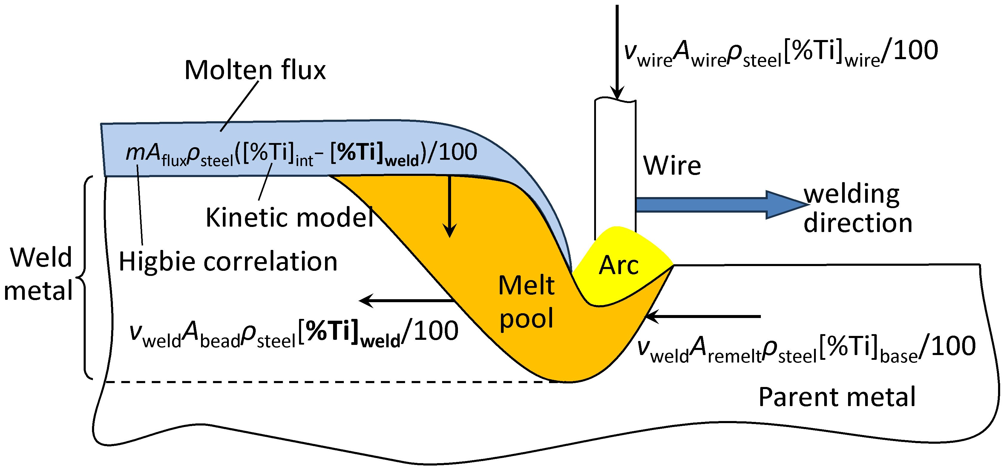
This work tested whether the kinetic and thermodynamic principles of the reaction between liquid metal and slag can be used to quantify the transfer of titanium to weld metal during submerged-arc welding (SAW). The summary presented here mainly draws on the review of Sengupta et al. [1] and the work of Mitra and Eagar [2]. In SAW (see Figure 1), metal is transferred from the wire to the melt pool as droplets that pass through the arc plasma. Multiple reactions are possible in the arc cavity, including the decomposition of oxides (like MnO and SiO₂) and the evaporation of fluorides like SiF₄. However, based on the work of Mitra and Eagar, it appears that the droplet–arc reactions mainly control the transfer of oxygen to the weld metal, whereas the recovery of alloying elements is established by the reactions between the weld metal and slag. As an example of the success of the Mitra and Eagar approach, the practically observed low recovery of chromium is consistent with the mechanism, and is driven by the strong equilibrium partitioning of chromium into the slag [2]. As will be shown, titanium also partitions strongly into the welding slag.

Titanium at concentrations in weld metal greater than 45 ppm [3] promotes the formation of acicular ferrite (AF). Acicular (“needlelike”) ferrite is an intragranular transformation product, where the ferrite nucleates on inclusions, with characteristic impingement of the ferrite grains giving a fine microstructure [4]. The formation of acicular ferrite in weld metal improves its toughness [3]. The effect of titanium on the formation of acicular ferrite has been linked to the compositions of oxide inclusions in solidified weld metal, with a higher titanium concentration promoting acicular ferrite nucleation [5]. However, acicular ferrite can also form in welds that do not contain any titanium; faster cooling and higher manganese concentrations promote acicular ferrite, with this being the main transformation product in steels with 1.3–1.8% Mn [3].

The equations in Figure 1 summarize the steps that are taken to enable titanium transfer to and from weld metal: titanium is melted into the weld pool from a continuously fed wire (with cross-sectional area A_wire and feed rate v_wire) and from the parent metal; the volumetric rate of melting of the parent metal or a previous pass is given by the product of the welding speed (v_weld) and the cross-sectional area (perpendicular to the welding direction) of the remelted region of the parent metal (A_remelt). Titanium is transferred between the melt pool and the slag at a rate that is proportional to the mass transfer coefficient of steel to slag (m), the contact area between the melt pool and slag (A_flux) and the titanium concentration difference between the bulk of the weld metal and at the metal–slag interface. At a steady state, the rate at which titanium enters the melt pool is equal to the rate at which titanium is removed from the melt pool by the solidification reaction. This equality allows calculation of the steady-state titanium concentration in the weld metal, if the titanium concentration at the metal–slag interface, [%Ti]_int, is known.

As reviewed in detail by Sengupta et al. [1], the available experimental data support the mechanism formulated by Mitra and Eagar [2], that the main role of the arc reactions is to cause oxygen transfer to the weld metal, whereas dilution and the steel–slag reaction control the concentrations of the other elements in the weld metal. Work on quantifying the reactions in the arc region has been reviewed in detail [6]; as shown in this thorough review, recent elucidation of reactions in the arc has focused on improved prediction of oxygen transfer. It was also emphasized that slag–metal reactions do not reach equilibrium [6]; this is the reason for the focus of the current work on quantifying the role of the kinetics of the slag–metal reactions.

Some recent work indicated a possible minor role of reactions in the arc cavity in titanium transfer: Wang et al. analyzed both quenched metal droplets and weld metal for submerged-arc weldments produced with fluxes, with titanium oxide concentrations ranging from zero to 25% [7]. Even at a high TiO₂ concentrationof 10% in the flux, there was zero pick-up of titanium by the weld metal, and the droplets contained just 23 ppm titanium. The fluxes used in the current work contained 1.3–1.6% TiO₂, which would suggest an even smaller role of titanium transfer to metal in the arc region. In fact—as shown later in this paper—the experimental results of Wang et al. [7] follow the predictions of the kinetic expressions developed in this work (which are summarized in Figure 1).

Based on the available literature on SAW reactions, the hypothesis that is tested in this work is that titanium transfer to the weld metal can be calculated based on these kinetic expressions for steel–slag reactions, without considering the detail of the arc reactions. The hypothesis is tested using submerged-arc deposits (using wire with and without Ti alloying), with additional information from laboratory equilibrium tests. This experimental work is described first, followed by the results of characterization of the weld flux, inclusion analysis, microstructures, and kinetic modeling. Part of the novelty of the current work is that it derives an analytical model that clearly shows the competing effects of dilution and steel–slag reactions on the steady-state concentration of titanium in the weld metal. In addition, microanalysis of the weld metal shows how the inclusion compositions respond to differences in the titanium concentration.

2. Experimental Work

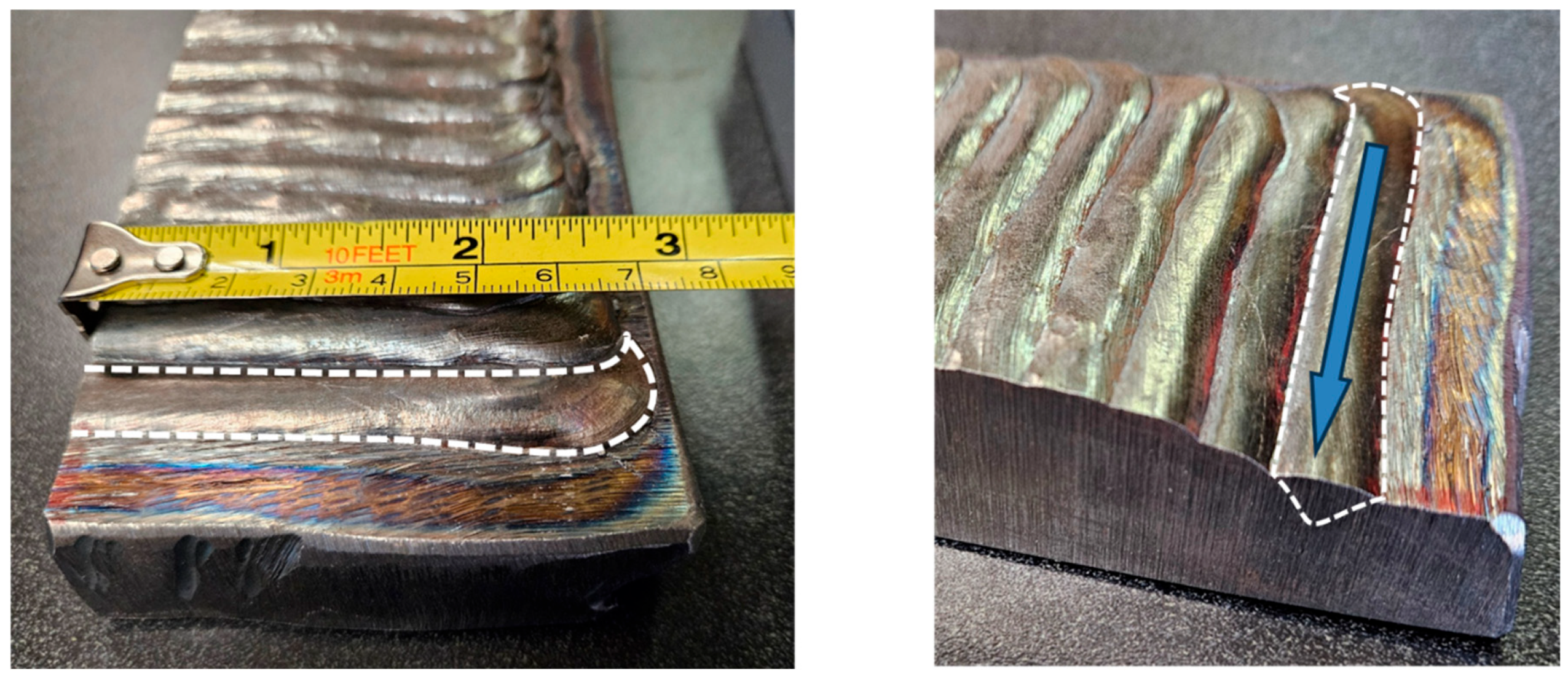
Weldments were prepared at the Hanover, PA ESAB research facility. Figure 2 shows a portion of one of the weldments, which were applied to a 20 mm thick base plate. To allow for chemical analysis of each layer, part of the first layer was not covered by the weld beads of the second pass. Similarly, part of the second layer was not covered by the third layer. The composition of each layer was subsequently measured (at ESAB Hanover) using optical emission spectroscopy (with LECO analysis for carbon). The measured compositions of the base plate, wire, and weld deposits are given in Table 1. The same weld flux was used for the weldments produced with the Ti-free and Ti-alloyed wires. The welding parameters are listed in Table 2. Used and unused weld fluxes were analyzed with x-ray fluorescence (XRF); the compositions are reported in Table 3.

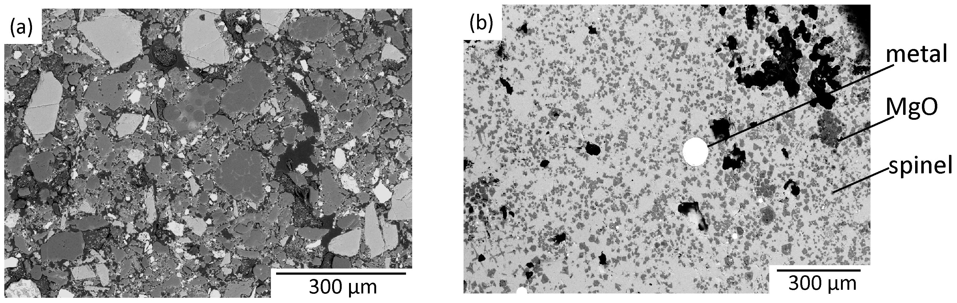
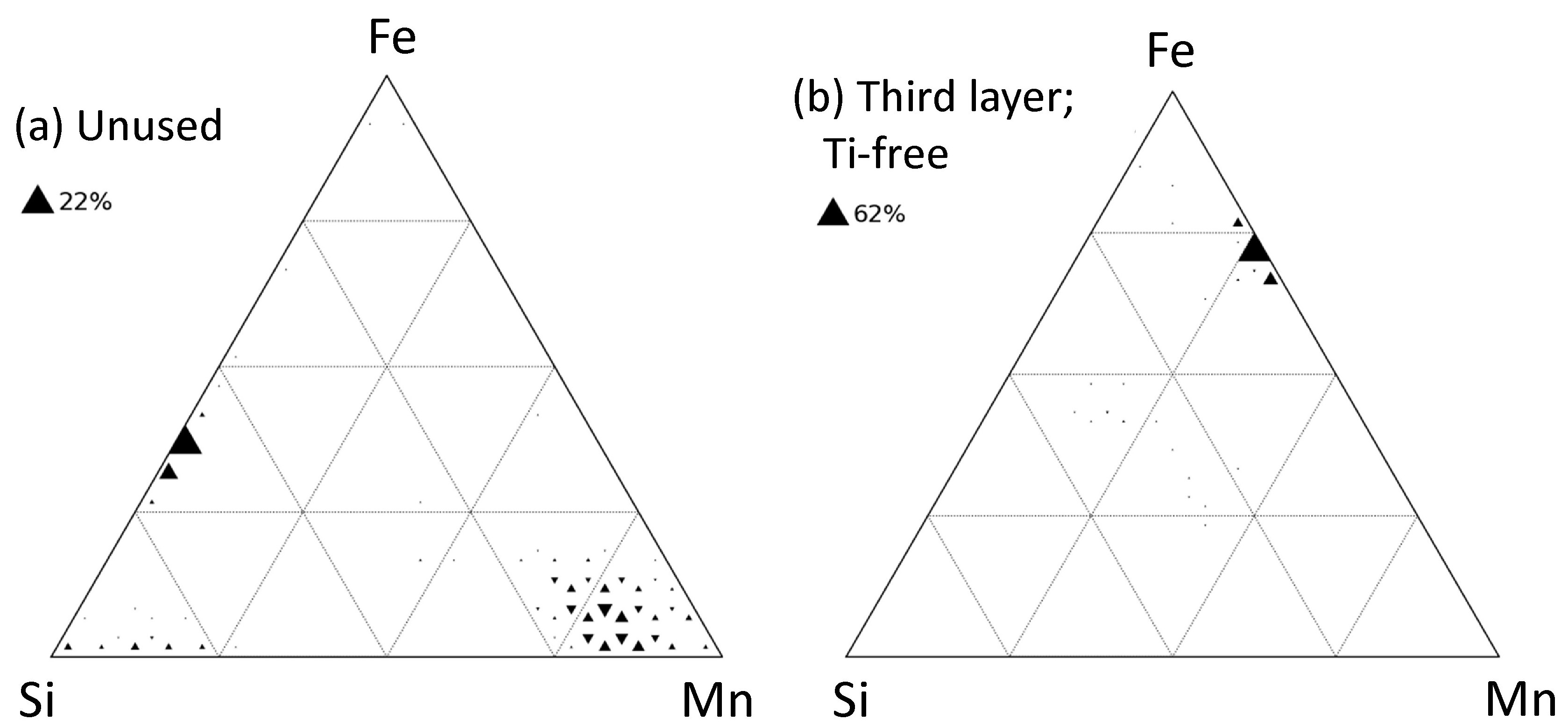
As shown below, the weld flux included ferroalloy powders (containing metallic Mn and Si). Since XRF analysis identifies only elemental compositions, the metallic Mn and Si in the flux are reported as MnO and SiO₂.

Slag (flux that had melted) was recovered from the melts, cross-sections were polished, and they were examined by scanning electron microscopy with energy-dispersive X-ray spectroscopy (SEM-EDS), Phenom ParticleX, NanoScience Instruments, Phoenix, AZ, USA to measure approximate elemental compositions of phases observed in the molten flux.

Automated feature analysis by SEM-EDS was used to measure the area fraction and elemental compositions of metal droplets in the slag, and of oxide inclusions in the weld metal, using the procedure described previously in [8,9].

Figure 2. Two views of one portion of the three-layer submerged-arc weldments (sectioned by band saw after welding). In the image on the right, the arrow indicates the welding direction. In both images, the white broken line outlines the bead deposited during the first pass.

Figure 2. Two views of one portion of the three-layer submerged-arc weldments (sectioned by band saw after welding). In the image on the right, the arrow indicates the welding direction. In both images, the white broken line outlines the bead deposited during the first pass.

Table 1. Compositions (mass basis) of the base plate and wire used for welding, as well as of the first and last layers produced with the Ti-free and Ti-alloyed wire.

	%C	%Mn	%Si	%Al	%Ti	ppm B
Base plate	0.21	1.21	0.26	0.037	0.000	0
Ti-free wire	0.09	1.06	0.13	0.0002	0.000	3
Weld metal: first layer	0.11	1.52	0.27	0.054	0.000	15
Weld metal: third layer	0.074	1.72	0.30	0.017	0.000	17
Ti-alloyed wire	0.07	1.57	0.26	0.012	0.140	110
Weld metal: first layer	0.12	1.65	0.32	0.043	0.014	30
Weld metal: third layer	0.07	2.02	0.39	0.018	0.022	43

Table 1. Compositions (mass basis) of the base plate and wire used for welding, as well as of the first and last layers produced with the Ti-free and Ti-alloyed wire.

	%C	%Mn	%Si	%Al	%Ti	ppm B
Base plate	0.21	1.21	0.26	0.037	0.000	0
Ti-free wire	0.09	1.06	0.13	0.0002	0.000	3
Weld metal: first layer	0.11	1.52	0.27	0.054	0.000	15
Weld metal: third layer	0.074	1.72	0.30	0.017	0.000	17
Ti-alloyed wire	0.07	1.57	0.26	0.012	0.140	110
Weld metal: first layer	0.12	1.65	0.32	0.043	0.014	30
Weld metal: third layer	0.07	2.02	0.39	0.018	0.022	43

Table 2. Welding parameters used for the multipass welds.

Wire	Diameter (mm)	Current (A)	Voltage (V)	Speed (mm/s)	Heat Input (kJ/mm)
Ti-free	3.18	480	28.5	8.68	1.58
Ti-alloyed	3.97	580	29	12.07	1.40

Table 2. Welding parameters used for the multipass welds.

Wire	Diameter (mm)	Current (A)	Voltage (V)	Speed (mm/s)	Heat Input (kJ/mm)
Ti-free	3.18	480	28.5	8.68	1.58
Ti-alloyed	3.97	580	29	12.07	1.40

Table 3. Concentrations (in mass percentages) of the main components in unused weld flux, and molten flux recovered from weldments produced with the Ti-free and Ti-alloyed wires. For the used fluxes, the first, second and third layers are indicated by A, D and G.

Sample	%CaF2	%CaO	%MgO	%Al2O3	%SiO2	%TiO2	%MnO
Unused	26.0	12.6	14.3	17.4	17.0	1.6	11.1
Slag: Ti-free wire A	22.0	8.0	23.0	20.0	17.4	1.3	8.3
Slag: Ti-free wire D	21.8	8.0	23.1	19.9	17.7	1.3	8.2
Slag: Ti-free wire G	23.5	6.7	24.5	18.9	17.2	1.3	8.0
Slag: Ti-alloyed wire A	17.9	13.4	21.5	18.7	16.8	1.8	9.9
Slag: Ti-alloyed wire D	22.3	7.8	22.5	19.6	17.5	1.6	8.6
Slag: Ti-alloyed wire G	25.1	4.9	23.3	19.7	17.4	1.6	8.0

Table 3. Concentrations (in mass percentages) of the main components in unused weld flux, and molten flux recovered from weldments produced with the Ti-free and Ti-alloyed wires. For the used fluxes, the first, second and third layers are indicated by A, D and G.

Sample	%CaF2	%CaO	%MgO	%Al2O3	%SiO2	%TiO2	%MnO
Unused	26.0	12.6	14.3	17.4	17.0	1.6	11.1
Slag: Ti-free wire A	22.0	8.0	23.0	20.0	17.4	1.3	8.3
Slag: Ti-free wire D	21.8	8.0	23.1	19.9	17.7	1.3	8.2
Slag: Ti-free wire G	23.5	6.7	24.5	18.9	17.2	1.3	8.0
Slag: Ti-alloyed wire A	17.9	13.4	21.5	18.7	16.8	1.8	9.9
Slag: Ti-alloyed wire D	22.3	7.8	22.5	19.6	17.5	1.6	8.6
Slag: Ti-alloyed wire G	25.1	4.9	23.3	19.7	17.4	1.6	8.0

Laboratory tests

The distribution of titanium between metal and slag was measured for MgO-saturated slag (similar in composition to weld flux), contained in a MgO crucible (58 mm ID) and inductively heated in a graphite susceptor under an argon atmosphere. The same procedure and experimental setup as described in detail in previous work was employed, ref. [10] using pure metals to make up the steel composition, and using pre-melted slag. A simplified flux composition was used, aiming for double-saturation with periclase (for compatibility with the crucible) and magnesia spinel (since this phase was found in the solidified slag from the welding tests). The temperature was monitored with a B-type thermocouple (in an alumina sheath), with its tip placed just above the slag. Each experiment used approximately 350 g of steel and 100 g of slag.

Experiments were conducted at 1600 °C and 1700 °C for a single slag composition (with some variability between experiments) and target steel compositions of 0.2% Si and 0.3% Si. After the experiment, the steel and slag were recovered from the MgO crucible. Steel samples were analyzed by ICP-MS, and slags by XRF. The compositions of the steel and flux after equilibration are summarized in Table 4 and Table 5.

The basicity index (in the slag composition table) was calculated using the International Institute of Welding (IIW) expression [11]; for the components considered here, it is given by

$$\mathrm{B}\mathrm{I}={\displaystyle \frac{\left(\%\mathrm{C}\mathrm{a}\mathrm{O}\right)+\left(\%\mathrm{C}\mathrm{a}{\mathrm{F}}_2\right)+(\%\mathrm{M}\mathrm{g}\mathrm{O})}{\left(\%\mathrm{S}\mathrm{i}{\mathrm{O}}_2\right)+0.5\left(\%\mathrm{A}{\mathrm{l}}_2{\mathrm{O}}_3\right)+0.5\left(\%{\mathrm{T}\mathrm{i}\mathrm{O}}_2\right)}}(\mathrm{m}\mathrm{a}\mathrm{s}\mathrm{s} \mathrm{p}\mathrm{e}\mathrm{r}\mathrm{c}\mathrm{e}\mathrm{n}\mathrm{t}\mathrm{a}\mathrm{g}\mathrm{e}\mathrm{s})$$

(1)

Table 4. Experimentally measured steel compositions after equilibration with simulated weld flux (mass percentages unless otherwise indicated).

Run	Mg	Al	Si	Ti	Ca
EW1 (1600 °C)	<0.5 ppm	0.00037	0.21	0.0014	<5 ppm
EW2 (1700 °C)	<0.5 ppm	0.00065	0.20	0.00083	<5 ppm
EW3 (1600 °C)	<0.5 ppm	0.0014	0.27	0.0025	0.0009
EW4 (1700 °C)	<0.5 ppm	0.0021	0.30	0.0038	0.0009

Table 4. Experimentally measured steel compositions after equilibration with simulated weld flux (mass percentages unless otherwise indicated).

Run	Mg	Al	Si	Ti	Ca
EW1 (1600 °C)	<0.5 ppm	0.00037	0.21	0.0014	<5 ppm
EW2 (1700 °C)	<0.5 ppm	0.00065	0.20	0.00083	<5 ppm
EW3 (1600 °C)	<0.5 ppm	0.0014	0.27	0.0025	0.0009
EW4 (1700 °C)	<0.5 ppm	0.0021	0.30	0.0038	0.0009

Table 5. Experimentally measured slag compositions after equilibration (mass percentages), with the basicity index.

Run	%CaF2	%CaO	%MgO	%Al2O3	%SiO2	%TiO2	BI
EW1	19.2	10.3	30.5	19.5	18.4	2.1	2.1
EW2	19.6	9.2	30.9	20.5	17.9	1.9	2.1
EW3	18.9	9.1	30.9	19.1	20.5	1.5	1.9
EW4	19.7	9.1	33.4	19.0	17.1	1.7	2.3

Table 5. Experimentally measured slag compositions after equilibration (mass percentages), with the basicity index.

Run	%CaF2	%CaO	%MgO	%Al2O3	%SiO2	%TiO2	BI
EW1	19.2	10.3	30.5	19.5	18.4	2.1	2.1
EW2	19.6	9.2	30.9	20.5	17.9	1.9	2.1
EW3	18.9	9.1	30.9	19.1	20.5	1.5	1.9
EW4	19.7	9.1	33.4	19.0	17.1	1.7	2.3

The apparent equilibrium constant (expressed in terms of mass percentages) was used to summarize the results, assuming that redox conditions are controlled by the Si-SiO₂ couple as expressed by Equation (2).

The assumption behind this expression is that the majority of titanium in the slag is in tetravalent form (TiO₂), which appears reasonable based on the results for ladle metallurgy conditions. [12] However, the concentration of titanium oxide in the slag is represented by “TiO₂” in the expression, to emphasize that some of the titanium would be present in lower oxidation states.

In Equation (2), species in round parenthesis are dissolved in the slag, and square brackets indicate solutes in the liquid steel.

$$C_{\mathrm{S}\mathrm{i}-\mathrm{T}\mathrm{i}}={\displaystyle \frac{\left({\mathrm{“}\%\mathrm{T}\mathrm{i}\mathrm{O}}_2\mathrm{”}\right)\left[\%\mathrm{S}\mathrm{i}\right]}{\left({\%\mathrm{S}\mathrm{i}\mathrm{O}}_2\right)\left[\%\mathrm{T}\mathrm{i}\right]}}$$

(2)

The values of the apparent equilibrium constant (C_Si-Ti) for all the experiments are summarized in

Table 6. Values of the apparent equilibrium constant C_Si-Ti for the equilibrium experiments and as predicted using the available thermodynamic data.

Run	CSi-Ti
	Experiment	Calculated
EW1 (0.2% Si, 1600 °C)	17	17
EW2 (0.2% Si, 1700 °C)	25	21
EW3 (0.3% Si, 1600 °C)	8.1	16
EW4 (0.3% Si, 1700 °C)	8.0	19

. Also shown in the table are the values of the apparent equilibrium constant calculated for these experimental conditions, using FactSage 8.3 with the liquid steel solution model from the FTmisc database, and the liquid slag (SLAGA), monoxide and spinel models from the FToxid database [13].

3. Results and Discussion

3.1. Characterization of Weld Flux

The unused flux contained a mixture of powdered oxides, fluorides and carbonates, in addition to ferroalloy particles (Figure 3a). Except for the region next to unmelted flux, the used flux appeared homogeneous, with the same phases present at different distances from the weld metal: the solidified flux contained some solidified metal droplets in a fine-grained matrix that also contained larger oxide particles—mainly MgO and magnesium spinel (Figure 3b). Ferroalloy powders were added as deoxidants to the flux [14], and also contribute to the weld metal composition. Microanalysis of the ferroalloy powders in the unused flux showed these to be mainly ferrosilicon- and Mn-rich (Figure 4). Table 1 illustrates that the weld metal has a higher concentration of Si and Mn than both the base plate and the welding wire, indicating that the ferroalloy powders transferred these elements to the weld metal. The droplets remaining in the flux after welding generally have lower concentrations of Mn and Si than the average of the original ferroalloy powders (Table 7 and Figure 4), also illustrating the role of the ferroalloy powders as deoxidants. In Figure 4 the compositions are shown as ternary proportional symbol plots, with the size of each the triangle scaled in proportion to the number of inclusions that fall in a particular triangle; the percentage in the legend is the number fraction of inclusions represented by the largest triangle [15].

Figure 3. Representative back-scattered electron images of (a) unused and (b) used weld flux, showing the presence of metallic particles (brightest regions) in both flux samples, as well as oxide phases in the solidified flux.

Figure 3. Representative back-scattered electron images of (a) unused and (b) used weld flux, showing the presence of metallic particles (brightest regions) in both flux samples, as well as oxide phases in the solidified flux.

Table 7. Area-averaged compositions (mole fractions) of the metal particles in unused and used flux. “A”, “D” and “G” refer to the flux recovered from the first, second and third weld layers.

Flux Sample	Fe	Mn	Si
Unused	0.10	0.61	0.29
Ti-alloyed wire A	0.43	0.30	0.28
Ti-alloyed wire D	0.29	0.25	0.46
Ti-alloyed wire G	0.37	0.53	0.10
Ti-free wire A	0.57	0.25	0.18
Ti-free wire D	0.31	0.56	0.13
Ti-free wire G	0.71	0.27	0.02

Table 7. Area-averaged compositions (mole fractions) of the metal particles in unused and used flux. “A”, “D” and “G” refer to the flux recovered from the first, second and third weld layers.

Flux Sample	Fe	Mn	Si
Unused	0.10	0.61	0.29
Ti-alloyed wire A	0.43	0.30	0.28
Ti-alloyed wire D	0.29	0.25	0.46
Ti-alloyed wire G	0.37	0.53	0.10
Ti-free wire A	0.57	0.25	0.18
Ti-free wire D	0.31	0.56	0.13
Ti-free wire G	0.71	0.27	0.02

Figure 4. Measured composition distribution (molar basis; proportional symbol map) of (a) metal particles in unused flux and (b) metal droplets in the used flux (example shown is for the third layer deposited using Ti-free wire). The decrease in the concentration in Mn and Si in the used flux is clear.

Figure 4. Measured composition distribution (molar basis; proportional symbol map) of (a) metal particles in unused flux and (b) metal droplets in the used flux (example shown is for the third layer deposited using Ti-free wire). The decrease in the concentration in Mn and Si in the used flux is clear.

3.2. Inclusion Analyses and Weld Metal Microstructures

As shown in Table 1, the largest difference in weld metal composition was found between the first layer deposited with Ti-free wire (zero titanium found in the weld by optical emission spectroscopy) and the third layer deposited using Ti-alloyed wire (0.022% Ti). These two extreme cases (identified as samples A2 and B6 respectively) were used to study possible links between the composition of the weld metal, inclusions, and weld metal microstructure. The inclusion size distribution and total area fraction are similar for the two cases (Figure 5). The total oxide area fraction (around 1000 ppm) can be used to estimate an approximate concentration of bound oxygen in the welds: if the inclusions are approximated as Mn₂SiO₄ with a density of 4.12 g/cm³ [16] and oxygen mass fraction of 0.32 (based on stoichiometry), and taking the matrix to be pure Fe with a density of 7.87 g/cm³, the mass fraction of oxygen in the steel is given by 0.32 × 4.12/7.87 = 0.166 times the volume fraction. Since the area fraction on a two-dimensional plane is equal to the volume fraction [17], the analyzed inclusion area fraction of 1000 ppm corresponds to an oxygen mass fraction in the steel of approximately 170 ppm. In line with the similarity of the size distributions, the inclusions appear similar in the two weld metal samples (Figure 6).

However, the average compositions of the inclusions were quite different: given the higher Ti concentration in weldment B6, a higher titanium oxide concentration was expected to arise from steel-inclusion reactions, and this is what was found (Table 8). This compositional difference was confirmed by manual EDS analysis on individual inclusions exposed by deep-etching of the steel matrix (Figure 7).

Figure 5. Cumulative size distributions of the oxide inclusions in the first layer deposited with Ti-free wire (A2), and the third layer deposited with the Ti-alloyed wire (B6); the size distributions are similar.

Figure 5. Cumulative size distributions of the oxide inclusions in the first layer deposited with Ti-free wire (A2), and the third layer deposited with the Ti-alloyed wire (B6); the size distributions are similar.

Figure 6. Representative backscattered electron images of oxide inclusions (black dots) in the weld metal with (a) low and (b) the highest titanium concentrations, as seen on polished sections.

Figure 6. Representative backscattered electron images of oxide inclusions (black dots) in the weld metal with (a) low and (b) the highest titanium concentrations, as seen on polished sections.

Table 8. Average compositions (mass percentages) of oxide inclusions in weld metal with low and the highest Ti concentrations.

Sample	%MnO	%TiO2	%SiO2	%Al2O3
A2 (low Ti)	30	3	24	43
B6 (highest Ti)	28	40	9	23

Table 8. Average compositions (mass percentages) of oxide inclusions in weld metal with low and the highest Ti concentrations.

Sample	%MnO	%TiO2	%SiO2	%Al2O3
A2 (low Ti)	30	3	24	43
B6 (highest Ti)	28	40	9	23

The images in Figure 7 were obtained by subjecting polished samples to electrolytic deep-etching (at approximately 1 A/cm² for 60 s) using anhydrous methanol containing 10% acetylacetone and 1% tetramethylammonium chloride [18]. This procedure etches out ferrite (producing facets), but does not attack cementite, or oxide and sulfide inclusions. In addition to revealing the inclusions and cementite, the resulting micrographs (Figure 7) show that the microstructures are similar for the weld metal with higher and lower titanium concentrations. Vickers hardness tests on polished samples also gave similar values for the weld metal with low and highest titanium concentrations (values given in Figure 7). The main microstructural component appears to be acicular ferrite [4], with possible nucleation of ferrite from an oxide inclusion visible in Figure 7a.

Figure 7. Deep-etched samples, showing examples of weld metal microstructure (at higher and lower magnifications) and oxide inclusions in weld metal with (a) low and (b) the highest titanium concentrations. The measured composition of the largest inclusion in the field of view is shown, as is the average Vickers hardness of the weld metal (with a 95% confidence interval).

Figure 7. Deep-etched samples, showing examples of weld metal microstructure (at higher and lower magnifications) and oxide inclusions in weld metal with (a) low and (b) the highest titanium concentrations. The measured composition of the largest inclusion in the field of view is shown, as is the average Vickers hardness of the weld metal (with a 95% confidence interval).

In line with the similar, fine microstructure visible after deep etching (Figure 7), optical microscopy did not show any clear features, or differences between the welds with higher and lower titanium concentrations (Figure 8). The images in Figure 8 were obtained after etching with sodium metabisulfite; Nital and saturated aqueous picric acid yielded similar results.

While the lack of an effect of titanium on the weld microstructure was unexpected, possible reasons for the presence of acicular ferrite in the low-Ti case are as follows: First, while the titanium concentration was too low for accurate analysis by optical emission spectroscopy for the weldment prepared with zero-titanium wire (Table 1), the non-zero concentration of titanium oxide in the oxide inclusions (Table 8) indicates that the weld metal does contain some titanium. Second, while titanium promotes acicular ferrite, it is not essential; the high manganese concentration in the weld metal (Table 1) is higher than the reported threshold of 1.3% Mn needed to form acicular ferrite without Ti alloying [3].

Figure 8. Examples of optical micrographs of weld metal (etched for 4 min with 10% aqueous picric acid). There is no evident difference in the microstructure between (a) the lower-titanium weld metal (a,b) the higher-titanium weld metal.

Figure 8. Examples of optical micrographs of weld metal (etched for 4 min with 10% aqueous picric acid). There is no evident difference in the microstructure between (a) the lower-titanium weld metal (a,b) the higher-titanium weld metal.

4. Kinetic Models

4.1. Titanium Recovery: Reaction Equilibrium

Equilibrium experiments and thermodynamic calculations (Table 6) showed similar values of the apparent equilibrium constant (C_Si-Ti) in the range 8–25, with little or no difference between 1600 °C and 1700 °C. However, the experimental values show an unexplained apparent effect of [%Si], with the ~0.3% Si runs giving lower values of C_Si-Ti. The apparent equilibrium constant should be independent of [%Si] if the activity of (SiO₂) and the activity coefficients of [Si], [Ti] and (TiO₂) are constant. A decrease in C_Si-Ti with increased Si is the opposite of the expected effect if a significant proportion of the titanium oxide in the mold flux was trivalent rather than tetravalent. The apparent experimental trend is currently unexplained, and might reflect the difficulty of accurately analyzing the low concentrations of Ti in the metal (8–40 ppm for these experiments; see Table 4).

Despite the uncertainty of the experimental results, the comparison of the experimental and calculated titanium distributions does indicate that calculations using the specific FactSage databases (FTmisc for liquid metal and FToxid for slag) can be used to predict the titanium distribution under SAW conditions.

In any case, some uncertainty in the titanium equilibrium has little effect on the calculated titanium recovery, because the equilibrium recovery of titanium in the metal is very low. This is illustrated by the titanium distribution coefficient between slag and steel (L_Ti):

$$L_{\mathrm{T}\mathrm{i}}={\displaystyle \frac{\left(\%\mathrm{T}\mathrm{i}\right)}{\left[\%\mathrm{T}\mathrm{i}\right]}}={\displaystyle \frac{48}{80}}{\displaystyle \frac{\left({\%\mathrm{S}\mathrm{i}\mathrm{O}}_2\right)}{\left[\%\mathrm{S}\mathrm{i}\right]}}{C}_{\mathrm{S}\mathrm{i}-\mathrm{T}\mathrm{i}}$$

(3)

In Equation (3), the factor 48/80 is the ratio between the molar masses of Ti and TiO₂. Typical values of C_Si-Ti ≈ 20, (%SiO₂) = 16%, and [%Si] = 0.2% give L_Ti ≈ 960. The very large distribution coefficient shows the strong tendency of titanium to be oxidized to the slag; for a typical value of (%TiO₂) = 1.6, the equilibrium concentration of Ti in the steel is [%Ti] ≈ 0.001%.

This low equilibrium concentration of titanium (10 ppm) reflects the strong tendency of titanium to be oxidized out of the liquid weld metal during submerged-arc welding; recovery of titanium in the weld metal relies on minimizing the interaction between the weld metal and the slag. The kinetic simulations support this conclusion, as shown below.

4.2. Governing Equations

The rate equations for the transfer of titanium into and out of the melt pool are given in Figure 1. As noted earlier, arc reactions are not explicitly considered in these expressions. Following the approach of Mitra and Eagar, [2] the assumption is that flux–steel reactions establish the steel composition, and the arc only influences such reactions by controlling oxygen transfer to the melt. Because the equilibrium concentration of titanium is so low, such oxygen transfer (which was considered in the full kinetic model) was found not to affect the titanium concentration in the weld significantly. As a result, the rate expressions do not consider any arc-related effects at all.

At steady state, the net rate of transfer of titanium into the melt pool equals the rate at which titanium is captured in the solidifying weld metal. A steady state should be approached when the wire has traveled a distance that is comparable to the melt pool length, which was estimated to be 41 mm for the conditions considered here (Table 9). The steady-state titanium concentration is practically useful, since the actual welds were tens of centimeters in length in this work (and also in typical welding fabrication).

By considering the transfer rates of titanium into and out of the melt pool, the steady-state titanium concentration is represented by the following expression:

$${\left[\%\mathrm{T}\mathrm{i}\right]}_{\mathrm{w}\mathrm{e}\mathrm{l}\mathrm{d}}={\displaystyle \frac{{v\left(\right[\%\mathrm{T}\mathrm{i}]}_{\mathrm{w}\mathrm{i}\mathrm{r}\mathrm{e}}{A}_{\mathrm{c}\mathrm{a}\mathrm{p}}+{[\%\mathrm{T}\mathrm{i}]}_{\mathrm{b}\mathrm{a}\mathrm{s}\mathrm{e}}{A}_{\mathrm{r}\mathrm{e}\mathrm{m}\mathrm{e}\mathrm{l}\mathrm{t}})+{m_{\mathrm{w}\mathrm{e}\mathrm{l}\mathrm{d}}\left[\%\mathrm{T}\mathrm{i}\right]}_{\mathrm{i}\mathrm{n}\mathrm{t}}{A}_{\mathrm{f}\mathrm{l}\mathrm{u}\mathrm{x}}}{v\left(A_{\mathrm{c}\mathrm{a}\mathrm{p}}+A_{\mathrm{r}\mathrm{e}\mathrm{m}\mathrm{e}\mathrm{l}\mathrm{t}}\right)+{m_{\mathrm{w}\mathrm{e}\mathrm{l}\mathrm{d}}A}_{\mathrm{f}\mathrm{l}\mathrm{u}\mathrm{x}}}}$$

(4)

In Equation (4), v is the welding speed, [%Ti]_wire is the titanium concentration in the wire and [%Ti]_base that in the remelted material (parent metal for the first pass, and remelted weld metal for subsequent passes), A_remelt is the cross-sectional area (perpendicular to the welding direction) of the remelted region and A_cap that of the weld deposit (reinforcement), m_weld is the mass transfer coefficient of titanium in the steel to the steel–slag interface, [%Ti]_int is the titanium concentration in the liquid steel at that interface, and A_flux is the contact area between liquid flux and liquid metal.

In using the expressions of Figure 1, both the liquid weld metal and the liquid flux are taken to be well-mixed, except for the boundary layers near the metal–flux interface; this is the same assumption used for other situations with kinetics controlled by mass transfer in steel and slag, such as ladle refining [19].

The remelt ratio (R, also known as the dilution ratio) is defined as the fraction of the melt pool cross-section that originates from remelted material (parent metal or previous weld passes):

$$R={\displaystyle \frac{A_{\mathrm{r}\mathrm{e}\mathrm{m}\mathrm{e}\mathrm{l}\mathrm{t}}}{A_{\mathrm{c}\mathrm{a}\mathrm{p}} + A_{\mathrm{r}\mathrm{e}\mathrm{m}\mathrm{e}\mathrm{l}\mathrm{t}}}}$$

(5)

The sum A_cap + A_remelt in Equation (5) is equal to the cross-sectional area of the weld metal, denoted as A_bead in Figure 1.

Since the wire that is transferred to the melt pool forms the cap on the weld, the area of the cap is related to the wire area and feed rate as follows:

$$v{A}_{\mathrm{c}\mathrm{a}\mathrm{p}}=v_{\mathrm{w}\mathrm{i}\mathrm{r}\mathrm{e}}{A}_{\mathrm{w}\mathrm{i}\mathrm{r}\mathrm{e}}$$

(6)

In Equation (6), v_wire is the wire feeding rate and A_wire the cross-sectional area of the wire (as also shown in Figure 1).

The mass transfer equation coefficient (m_weld) was estimated using the Higbie expression [20]:

$$m_{\mathrm{w}\mathrm{e}\mathrm{l}\mathrm{d}}=2\sqrt{{\displaystyle \frac{D}{\pi t_e}}}$$

(7)

In Equation (7), m_weld is the mass transfer coefficient, D the diffusivity of titanium in liquid steel (approximately 10⁻⁹ m²/s), and t_e the transient contact time between metal and slag. The surface renewal time (t_e) can be estimated as the half-width of the melt pool (approximately 8 mm, see Table 9) divided by the flow speed of steel in the weld metal. Estimates indicate that the speed is approximately 1 m/s, [21] giving an estimated mass transfer coefficient of 4 × 10⁻⁴ m/s.

Equation (4) reveals that [%Ti]_weld, the titanium concentration in the deposit, is the weighted average of the titanium concentrations in the wire, in the remelted base, and at the steel–slag interface. The weighting factors are the volumetric flow rates (given by vA for the wire and remelt, and m_weldA_flux for the interfacial concentration). To quantify these weighting factors, the cross-sectional area of the weld was approximated as two half-ellipses. This approximation gives the cross-sectional area as follows:

$$A_{\mathrm{w}\mathrm{e}\mathrm{l}\mathrm{d}}=A_{\mathrm{r}\mathrm{e}\mathrm{m}\mathrm{e}\mathrm{l}\mathrm{t}}+A_{\mathrm{c}\mathrm{a}\mathrm{p}}={\displaystyle \frac{\pi HW}{4}}$$

(8)

where H is the total depth of the weld pool (including both the remelt and the reinforcement) and W is the weld-pool width.

The contact area between the flux and the molten weld metal was approximated as a half-cylinder:

$$A_{\mathrm{f}\mathrm{l}\mathrm{u}\mathrm{x}}={\displaystyle \frac{\pi WL}{2}}$$

(9)

where L is the length of the melt pool.

In the calculation of the steady-state titanium concentration (Equation (4)), the weighting factor of the interfacial titanium concentration is m_weldA_flux and that of the substrate and wire titanium concentrations is vA_weld. Using values of the mass transfer coefficient in the molten metal (m_weld) and welding speed (v) from Table 9 gives the ratio of these weighting factors as m_weldA_flux/vA_weld = 0.3. This means that the (low) interfacial concentration of titanium has a similar (but slightly weaker) effect on the titanium concentration in the weld deposit to the titanium concentration in the substrate and wire. This weighting factor of the interfacial titanium concentration reflects the balance between the contact area between the weld metal and the flux (A_flux) being much larger than the weld cross-section (A_weld), by a ratio of about 9, in part balancing the large ratio (about 30) of welding speed to the mass transfer coefficient. Measures to decrease the contact area—for example, a narrower melt pool—would give higher titanium recovery to the metal, if other factors remain equal.

Table 9. Parameters used in the kinetic models.

Model Parameter	Value	Source
Welding speed (v)	12.1 mm/s	ESAB welding conditions
Weld bead width (W)	17.4 mm	ESAB measurement
Weld bead depth (H)	9.3 mm	ESAB measurement
Melt pool length (L)	41 mm	ESAB measurement
Remelt ratio (R)	0.8	Estimate from cross-sections
Liquid flux depth (hflux)	1.5 mm	Measured (this work)
Steel mass transfer coefficient (mweld)	0.4 mm/s	Estimate from the literature [20,21]
Slag mass transfer coefficient (mslag)	0.1 mweld	Previous work [19]
Liquid steel density	7000 kg/m3	Value for molten Fe
Liquid slag density	2500 kg/m3	Typical for liquid slag
Temperature	1600 °C	Liquidus + superheat

Table 9. Parameters used in the kinetic models.

Model Parameter	Value	Source
Welding speed (v)	12.1 mm/s	ESAB welding conditions
Weld bead width (W)	17.4 mm	ESAB measurement
Weld bead depth (H)	9.3 mm	ESAB measurement
Melt pool length (L)	41 mm	ESAB measurement
Remelt ratio (R)	0.8	Estimate from cross-sections
Liquid flux depth (hflux)	1.5 mm	Measured (this work)
Steel mass transfer coefficient (mweld)	0.4 mm/s	Estimate from the literature [20,21]
Slag mass transfer coefficient (mslag)	0.1 mweld	Previous work [19]
Liquid steel density	7000 kg/m3	Value for molten Fe
Liquid slag density	2500 kg/m3	Typical for liquid slag
Temperature	1600 °C	Liquidus + superheat

4.3. Analytical Model

Approximate values of the steady-state titanium concentration in the weld metal were obtained by taking the interfacial concentration of titanium ([%Ti]_int) to be equal to the equilibrium concentration for the reaction between the liquid steel and flux, with the equilibrium calculated as follows:

$${[\%\mathrm{T}\mathrm{i}]}_{\mathrm{e}\mathrm{q}\mathrm{u}\mathrm{i}\mathrm{l}\mathrm{i}\mathrm{b}\mathrm{r}\mathrm{i}\mathrm{u}\mathrm{m}}={\displaystyle \frac{{[\%\mathrm{T}\mathrm{i}]}_0}{1+L_{\mathrm{T}\mathrm{i}}\frac{W_{\mathrm{s}\mathrm{l}\mathrm{a}\mathrm{g}}}{W_{\mathrm{s}\mathrm{t}\mathrm{e}\mathrm{e}\mathrm{l}}}}}$$

(10)

In Equation (10), [%Ti]₀ is the total titanium mass entering the melt pool and molten flux from the wire, remelted base metal and flux, expressed as a percentage of the liquid steel mass, and W_slag/W_steel is the mass ratio of liquid flux to liquid metal. The mass ratio was calculated as 0.12, based on the densities of slag and steel and the measured thickness of the liquid flux (Table 9). [%Ti]₀ is calculated as follows:

$${[\%\mathrm{T}\mathrm{i}]}_0={(1-R)[\%\mathrm{T}\mathrm{i}]}_{\mathrm{w}\mathrm{i}\mathrm{r}\mathrm{e}}+{R[\%\mathrm{T}\mathrm{i}]}_{\mathrm{b}\mathrm{a}\mathrm{s}\mathrm{e}}+{\displaystyle \frac{48}{80}}{\displaystyle \frac{W_{\mathrm{s}\mathrm{l}\mathrm{a}\mathrm{g}}}{W_{\mathrm{s}\mathrm{t}\mathrm{e}\mathrm{e}\mathrm{l}}}}{\left({\%\mathrm{T}\mathrm{i}\mathrm{O}}_2\right)}_{\mathrm{f}\mathrm{l}\mathrm{u}\mathrm{x}}$$

(11)

For welds made with Ti-containing wire on low-Ti base plates (compositions in Table 1), with areas of remelt and reinforcement as given in Table 9, and a typical (%TiO₂)_flux of 1.6%, the equations give [%Ti]₀ = 0.14% and [Ti]_equilibrium = 0.0013%.

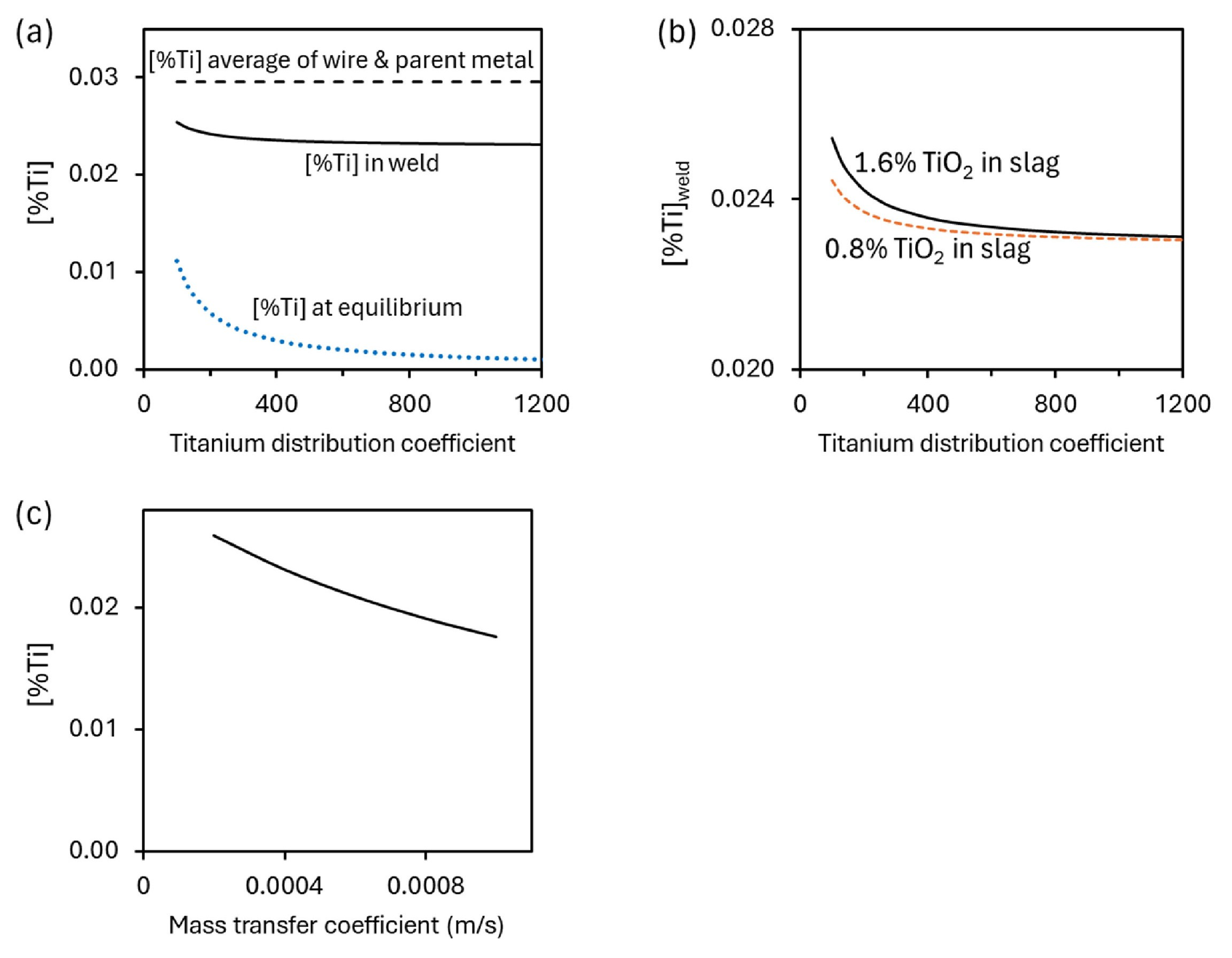
Examples of predictions of the analytical model (Figure 9) emphasize the lowequilibrium titanium concentration. The titanium concentration of the weld metal is between the equilibrium value and the weighted average of the wire and base compositions; the latter weighted average titanium concentration is itself low (compared with the wire composition) because of the high remelt ratio (about 80% for the welding conditions considered here). The results in Figure 9 suggest that changes in the titanium reaction equilibrium (by increasing [%Si] or (%TiO₂)_flux, or making basicity changes) would not be effective in increasing the titanium concentration in the weld metal—but lower dilution (if feasible) would have a strong effect. The results also show that stronger mass transfer in the melt pool would move the titanium concentration closer to the low equilibrium concentration.

The analytical approximation predicts a higher titanium concentration than the actual analysis of the weld deposit: The titanium concentration in the first pass deposited with Ti-alloyed wire was 0.014% (Table 1), compared with a prediction by the analytical model of around 0.02% (Figure 9). As shown in the next section, a small difference in the remelt ratio could account for this discrepancy (and, as shown in this section, increased mass transfer in the melt pool would have a similar effect).

Figure 9. Examples of the predictions of the analytical model, using the default values from Table 9, showing (a) the weak effect of a changed distribution coefficient, (b) the limited effect of increased titanium oxide additions to the flux, and (c) the effect of increased mass transfer in the melt pool on decreasing the titanium concentration in the melt pool. The results indicate that the titanium reaction is far from achieving equilibrium, and is not strongly affected by factors that change the equilibrium, including the distribution coefficient (a) and the titanium concentration in the flux (b).

Figure 9. Examples of the predictions of the analytical model, using the default values from Table 9, showing (a) the weak effect of a changed distribution coefficient, (b) the limited effect of increased titanium oxide additions to the flux, and (c) the effect of increased mass transfer in the melt pool on decreasing the titanium concentration in the melt pool. The results indicate that the titanium reaction is far from achieving equilibrium, and is not strongly affected by factors that change the equilibrium, including the distribution coefficient (a) and the titanium concentration in the flux (b).

4.4. Multicomponent Reaction Model

The analytical model is correct in principle (subject to the accuracy of the underlying assumptions), but its limitation is that it assumes that the interfacial concentration of titanium is the equilibrium concentration. In reality, the interfacial concentrations (of all elements, not just titanium) result from the multi-component reaction between the steel and slag, involving the transfer of not just titanium between the steel and slag, but also aluminum, silicon, manganese and oxygen. A full multicomponent model was constructed for more accurate predictions, using the following approach:

The reaction between the steel and slag was assumed to be under mass transfer control, with m_weld defining the mass transfer coefficient between the steel and the slag; as in previous work for ladle metallurgy, the corresponding mass transfer coefficient in the slag (m_slag) was assumed to be equal to 0.1m_weld. [19] The model was constructed by using a FactSage macro to calculate the transfer of Ti between steel and slag during each time step, and finding the interfacial compositions (in steel and slag) for each time step. The approach is similar to that used for ladle reactions, with the following differences: at each time step metal was added to the melt pool from the wire and remelt, and it was removed in solidified weld metal, and similarly, unreacted flux was added to the slag (and solidified flux removed from the slag). The same underlying constants (Table 9) were used as for the analytical calculations, with a time step of 0.5 s.

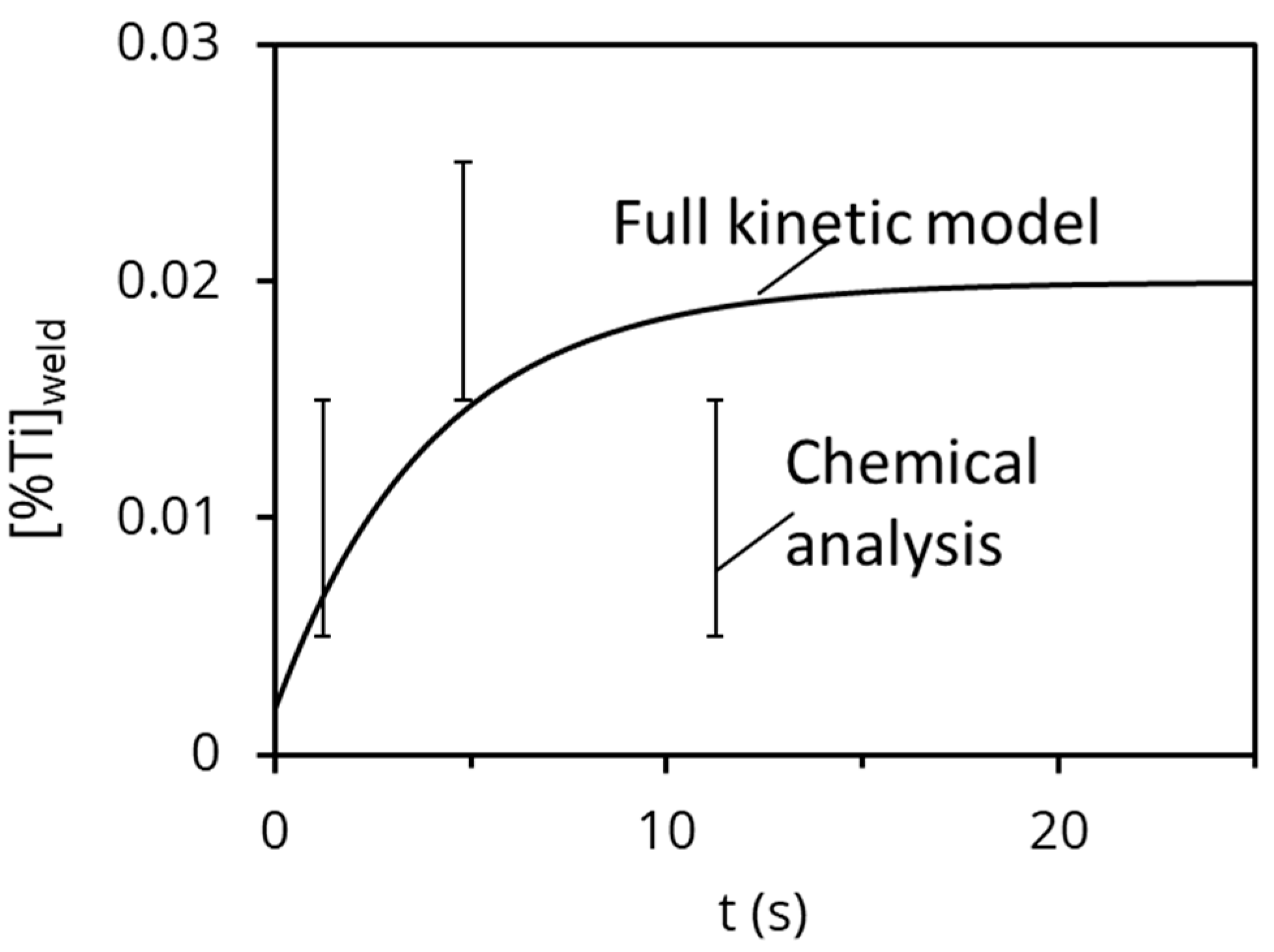
According to the multicomponent reaction model, the titanium concentration in the melt pool approaches the steady-state value within approximately 15 s (Figure 10). The predicted steady-state titanium concentration in the weld is approximately 0.020%, also higher than the experimental value for the first layer of weld deposit of 0.014% (Table 1), and similar to the predictions of the analytical model. The characteristic time for the development of the melt pool composition is the length of the melt pool divided by the welding speed, which is 3.4 s for the default conditions—in line with the time taken to approach a steady state, according to the model. For comparison with the model results, sections of the weld metal from the first pass were removed by electric discharge machining (EDM) and analyzed at an external laboratory. The results were reported to a precision of 100 ppm, limiting their usefulness, but do seem to support the model prediction of rapidly reaching a steady-state composition (Figure 10).

The predictions of the full kinetic model and the approximate analytical model agree closely because of the smaller effect of the reaction equilibrium on the titanium concentration in the weld metal (as also illustrated in Figure 9a). The full kinetic model fundamentally accounts for the oxidation and reduction reactions between all species at the steel–slag interface, but the equilibrium concentration of titanium is low in all cases, and small shifts in the equilibrium have little effect. In contrast, dilution of the wire by the base metal (the remelt ratio) has a strong effect.

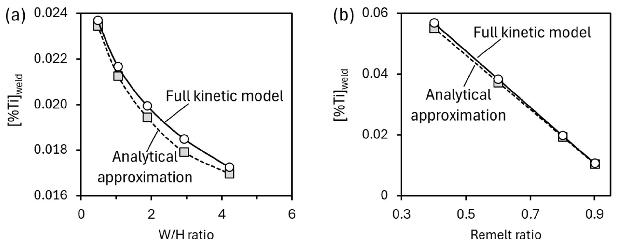
The dominant effect of dilution is demonstrated in Figure 11: Increasing the extent of reaction between the melt pool and the slag (by increasing the aspect ratio of the melt pool, expressed as W/H) does decrease the steady-state titanium concentration somewhat. (When testing the effect of the cross-sectional aspect ratio of the melt pool, the melt pool cross-sectional area was kept constant, as expected if the heat input remains the same.) However, the remelt ratio has a much stronger effect (Figure 11b): less dilution of the titanium-rich wire by the base metal (represented by a smaller remelt ratio) would give substantially higher titanium concentrations in the weld metal. (In these calculations, the cross-sectional area was also kept constant when adjusting the remelt ratio.)

Both the approximate analytical model and the full kinetic model predicted somewhat higher titanium concentrations in the weld metal than found experimentally. As the sensitivity analysis in Figure 9 indicates, a possible reason for the difference is a higher-than-estimated mass transfer coefficient; roughening of the steel–slag interface (under the influence of rapid flow) would have a similar effect. A higher mass transfer coefficient and an increased steel–slag reaction area would both cause the titanium concentration to approach the (low) equilibrium value more closely (as shown in Equation (4)). Given the dominant role of dilution and steel–flux reactions in setting the weld metal composition, uncertainty in the mass transfer conditions is a more likely explanation for the difference between predicted and actual titanium concentrations.

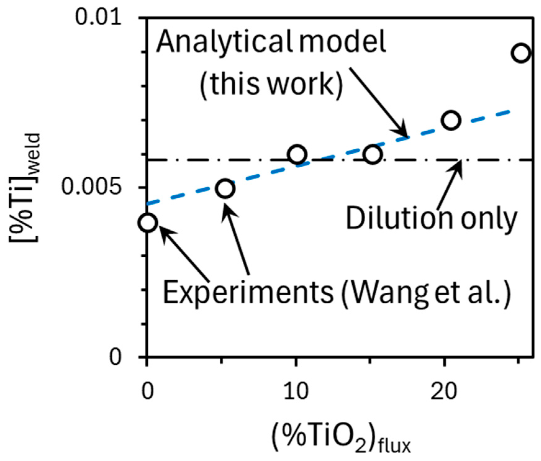
As a further test of the current approach, experimental results recently reported by Wang et al. [7] were compared with the predictions of the model developed in the current work. Wang et al. prepared single-bead welds with a dilution ratio of 0.53, using CaO-SiO₂-MnO-TiO₂ fluxes with constant (%SiO₂) = 30% and (%CaO) = 20%, and varying (%MnO) and (%TiO₂). In that work, the wire contained no titanium, and [%Ti] = 0.011% for the base metal. In the absence of other information, the weld pool dimensions and welding speed were taken to be the same as in the current work. Figure 12 shows that the analytical model (developed in the present work) predicted titanium concentrations in the weld metal that are close to the experimental results of Wang et al. for all except the case with the highest titanium oxide concentration in the flux. Notably, all the compositions remained close to the average composition of the parent metal and wire (calculated with the reported dilution ratio); this emphasizes the limited effect of chemical reaction on the titanium concentration in the weld metal, compared with the effect of dilution.

Because of the strong effect of dilution, the development of the titanium concentration in the weld metal during multipass welds would be strongly affected by welding conditions. For example, higher interpass temperatures would increase the melt pool size, with more dilution and less of an effect of titanium introduced in the wire on the weld metal titanium concentration. The importance of welding conditions is shown by the wide range of dilution ratios reported in the literature. At the lower end, Mitra stated that the dilution ratio can be as low as 0.45 [22], and the lowest dilution ratio in the work of Saini and Singh was 0.41 [23]; these are much lower than the estimated dilution ratio of 0.8 in the current work, showing the wide range of dilution during welding.

5. Conclusions

The kinetic model of titanium transfer during submerged-arc welding matches the observed low titanium recovery in the first weld bead. The low titanium recovery is a result of the relatively oxidizing conditions for titanium, yielding a large equilibrium distribution coefficient of titanium between the welding slag and the liquid steel in the melt pool. Factors that limit interaction between the metal and flux—such as narrower melt pools—should improve titanium recovery. The titanium concentration in the deposited weld metal is more strongly affected by the extent of dilution by base metal or previous passes. These results do support the hypothesis that considering only the reaction between liquid weld metal and flux—without considering the arc—gives a reasonable prediction of the titanium concentration of the weld deposit.

Conditions set by the reaction between the liquid weld metal and slag are strongly oxidizing towards titanium, with a large titanium distribution coefficient (around 1000) between slag and metal. This work predicts that changes in the distribution coefficient around this large value (for example, by adjusting the flux basicity) would not affect titanium recovery significantly. Instead, testing the effects of decreased dilution and less interaction between the weld metal and flux (by adjusting weld parameters) would be a promising avenue of future research. The analytical model indicates that the titanium concentration of the weld deposit is the weighted average of the titanium concentration at the metal–slag interface (contributing about 30%, for the assumed conditions) and the average of the wire and substrate compositions (weighted according to the remelt ratio, contributing about 70%). Since the lowequilibrium titanium concentration has the smaller weight, approaches that limit dilution appear to be most promising to increase the titanium concentration in the deposit.