A Reliability- and Energy-Aware Decision-Support Framework for Production–Maintenance Scheduling in Parallel CNC Machining Systems

Abstract

In parallel CNC machining systems, machine deterioration can simultaneously increase energy-related operating costs, affect delivery performance, and change the timing of preventive maintenance. This study develops a reliability- and energy-aware decision-support framework for production-maintenance scheduling in a two-machine parallel CNC cell. The model integrates priority sequencing, reliability-based machine assignment during decoding, degradation-dependent energy cost, tardiness penalties, and threshold-triggered preventive maintenance in a unified cost-minimization formulation. A normalized reliability index is updated by a short-horizon exponential degradation function, and the energy term is amplified when machines operate in degraded states. Preventive maintenance is triggered when post-job reliability falls below a specified threshold, restoring the machine’s condition for subsequent production or the next planning horizon. The computational study combines application-inspired machining instances, decoder-space full enumeration for small cases, repeated GA/PSO comparisons, a new algorithm-budget sensitivity experiment, and adapted OR-Library weighted-tardiness benchmarks. Across 270 paired budget-sensitivity runs, GA obtained a lower total cost in 265 cases, whereas PSO retained a shorter average runtime in the matched-budget experiments. Across 90 adapted public-benchmark comparisons, GA obtained a lower total cost in 86 cases. These results show that the framework generates feasible schedules and reveals energy–maintenance–tardiness trade-offs. The algorithmic findings are interpreted as a quality–time trade-off under the tested scalarized cost model, not as a claim of universal algorithmic superiority.

1. Introduction

Manufacturing is among the largest industrial consumers of electricity, and machining operations are widely recognized as a major driver of industrial energy demand. In parallel-machine environments, cutting and non-cutting activities, including spindle acceleration, coolant circulation, axis positioning, standby, and restart, all contribute to total energy use [1,2]. The financial impact is particularly important in precision sectors such as aerospace and automotive manufacturing, where high-power spindles and long cycle times make electricity a non-negligible component of unit cost [3]. Recent energy-aware scheduling studies reduce this burden by modifying machine assignment, sequencing, load balancing, idle periods, and on/off profiles [4]. Energy performance is also related to equipment condition: maintenance can restore machines to more efficient operating states, while wear and degradation increase spindle and feed power requirements [5]. In parallel CNC cells, decisions about job assignment and preventive maintenance therefore influence energy costs, reliability, and delivery performance simultaneously [6].

Despite this progress, a practical gap persists. Many planning systems still treat production scheduling and maintenance as separate problems, or they optimize energy in isolation from reliability. This siloed view struggles to answer day-to-day questions supervisors face in parallel-machine cells: Which jobs should start first on which machine today? When should PM be inserted to ensure recovery of the condition without jeopardizing the due windows? How do these choices jointly shape energy, delivery, and cost within a single shift? The literature points toward an answer to integrated production–maintenance optimization, but there remains a need for decision frameworks that (i) operate at shift resolution, (ii) respect non-preemptive processing with endogenous, condition-triggered PM, and (iii) expose energy–delivery–cost trade-offs in a way that is auditable and easy to implement on the shop floor [4].

This study is motivated by a typical parallel CNC machining cell in automotive e-axle production, where two identical turn–mill centers may be used to process gear- and bearing-type components for reduction gearboxes and differentials. Such machining operations usually involve relatively long cycle times, high spindle power, and strict delivery requirements. In this situation, equipment deterioration is not just a maintenance problem but also a scheduling problem: assigning more work to one machine may improve workload balance in the short term, but it can also accelerate reliability decay, increase energy-related operating costs, and increase the likelihood of preventive maintenance. Conversely, inserting maintenance too early may waste useful machine capacity and increase tardiness. Therefore, production scheduling and maintenance planning should not be treated as independent decisions in degradation-sensitive CNC machining environments.

Because complete shop-floor records cannot be publicly disclosed, this paper is presented as an application-inspired, reproducible computational study rather than a confidential industrial case report. The constructed machining instances represent typical CNC workpiece categories, such as gears, rings, couplings, and sleeves, with processing times selected to reflect realistic workload differences. Adapted OR-Library weighted-tardiness benchmarks are also used to reduce dependence on a single constructed data source. This design allows the proposed scheduling mechanism to be examined under controlled settings for due-date tightness, degradation, maintenance, and energy cost while keeping the experiments reproducible.

The literature review indicates three specific gaps. First, many energy-aware scheduling models treat power demand as a fixed or machine-specific coefficient, so the effect of deterioration on energy costs is not explicitly represented. Second, maintenance is often introduced as an external or periodic activity rather than as an endogenous event triggered by the reliability state created by the schedule itself. Third, parallel-machine studies frequently optimize assignment and sequencing without showing how the resulting reliability states affect energy, tardiness, and maintenance cost together. The present study addresses these gaps through a closed-loop model in which a priority sequence is decoded into machine schedules, reliability is updated after each job, energy cost depends on the entering reliability state, and PM is triggered by the resulting post-job reliability. The computational goal is to test feasibility, reproducibility, and trade-off behavior, rather than ranking all possible scheduling algorithms.

The remainder of the paper is organized as follows. Section 2 presents the problem setting, assumptions, notation, reliability-dependent energy-cost model, threshold-based PM logic, and GA/PSO solution procedures. Section 3 reports the computational experiments, including small-scale decoder-space enumeration validation, medium- and large-scale comparisons, statistical tests, sensitivity analysis, and validation on adapted public benchmarks. Section 4 concludes the study and discusses limitations and future extensions.

Modern manufacturing increasingly treats production scheduling as a systems-level problem in which throughput, delivery performance, energy consumption, and equipment health interact. In parallel-machine settings, research has shifted beyond classical makespan or tardiness objectives to energy-aware formulations that integrate load balancing, speed adjustment, and machine on/off control with preventive or condition-based maintenance. Hybrid models further embed degradation and opportunistic maintenance into dispatching, explicitly linking machine wear with power demand to couple availability and energy efficiency [7]. Current frameworks highlight the importance of event-triggered and hybrid scheduling systems that balance computational cost, resilience, and optimality [8]. Significantly, empirical data supports this connection: [9] showed a high correlation between energy consumption and machine dependability, demonstrating that deterioration increases unit energy consumption in addition to decreasing availability. This emphasizes the necessity of models that do not treat energy functions as static coefficients but rather as functions that depend on deterioration or reliability states. By facilitating concurrent processing and job-machine assignment, parallel machine scheduling (PMS) offers structural flexibility by distributing wear and balancing workload [10]. Building on this basis, energy-aware PMS frequently uses machine-specific coefficients, sequence-dependent setup durations, and physics-based power models to smooth demand and prevent unproductive idle states [11].

A second stream focuses on preventive and condition-based maintenance (PM/CBM). Rather than treating maintenance as an external stage, recent studies embed inspection intervals, variable processing speeds, or maintenance insertions directly into scheduling [12]. Industry 4.0 technologies have further enabled predictive maintenance through condition monitoring, data-driven decision support, and integrated production–maintenance planning [13,14]. Extensions consider demand uncertainty and multiple-machine interactions, while joint quality–maintenance models emphasize how degradation affects defect rates and overall cost [14].

The third stream addresses integrated production and maintenance scheduling. Recent studies have increasingly emphasized the coordination of production scheduling and maintenance under shared resources, sequence-dependent setups, and machine deterioration. For example, ref. [15] integrated preventive maintenance and production planning with sequence-dependent setup costs and times, while [16] proposed a joint scheduling approach for production and predictive maintenance activities. More recently, ref. [17] studied integrated maintenance and production scheduling for unrelated parallel machines with setup times. Methodological reviews further document the shift from classical parallel-machine scheduling to integrated assignment, sequencing, and maintenance-aware optimization [5]. Reliability-driven models also incorporate degradation directly into production and maintenance decisions, thereby aligning production planning, maintenance timing, and quality-related cost [18]. Despite substantial advances, several critical limitations persist in the literature on parallel-machine scheduling and its integration with energy and reliability. Many models treat degradation as exogenous (e.g., periodic PM), optimizing energy independently of equipment health, thereby misestimating power demand under wear and mistiming interventions [12]. Schedule-first, maintain-later approaches ignore feedback between task assignment and degradation; while locally effective, they often miss global optima across energy, tardiness, and maintenance [19]. Assumptions like constant failure rates understate the influence of load, speed, and duty cycles on wear and power draw [20]. Many studies scalarize via weighted sums or lexicographic rules, which under-represent state-triggered transitions and may yield unstable trade-offs [21]. Across these research streams, energy-aware scheduling with on/off strategies, speed control, and machine-reliability constraints has been investigated, particularly in single-machine environments [22]. Sustainable production-scheduling studies have also incorporated demand-response mechanisms, electricity tariffs, and carbon-policy considerations to evaluate the economic and environmental consequences of scheduling decisions [23]. Predictive-maintenance scheduling has further considered reliability characteristics that vary with the phase of the machine life cycle, showing that maintenance timing should reflect the evolving machine condition rather than a fixed external schedule [24]. Nevertheless, degradation-dependent energy models remain relatively limited, energy is often treated as an external cost in condition-based maintenance studies, and explicit energy–maintenance state coupling remains insufficiently addressed in parallel-machine scheduling.

These gaps motivate a reliability-driven, energy-aware PMS model that explicitly links degradation, energy use, maintenance timing, and tardiness. The novelty of this work is not any single component in isolation, since parallel-machine scheduling, reliability decay, preventive maintenance, and metaheuristic search are all established topics. Rather, the contribution lies in combining them into a transparent decision-support formulation for parallel CNC machining: reliability evolves endogenously from the decoded schedule, energy cost is amplified by the current reliability state, and PM is triggered by the same state variable that affects energy. The computational design further supports reproducibility through decoder-space enumeration checks, repeated stochastic runs, sensitivity analysis, and adapted public benchmark instances.

The following contributions made by this work advance the field:

• A reliability- and energy-aware scheduling formulation is developed for parallel CNC machining systems. The model integrates machine assignment, job sequencing, reliability degradation, energy-related operating cost, tardiness, and threshold-based preventive maintenance into a unified cost-minimization framework.
• A transparent degradation-dependent energy-cost structure is introduced. Instead of treating energy consumption as a fixed coefficient, the model links the energy amplification factor to machine reliability, thereby capturing the operational effect of degraded machine states on energy-related cost.
• A reproducible computational experiment design is provided. The numerical study combines application-inspired machining instances based on gear and bearing production with public OR-Library weighted tardiness benchmarks adapted to a two-machine environment.
• A GA-based solution procedure is developed and compared with PSO and decoder-space full enumeration on small instances. The comparison is used to evaluate implementation behavior, solution quality, runtime, and robustness under controlled settings, rather than to claim general superiority of one metaheuristic over all alternatives.
• The results provide managerial insights into how reliability thresholds, due-date tightness, maintenance timing, and sequencing decisions jointly influence energy, tardiness, and maintenance costs in parallel CNC machining systems.

2. Materials and Methods

2.1. Problem Setting and Assumptions

In this study, the energy consumption of each job is modeled as a function of both its processing time and the machine’s current reliability state. Let ${\sigma }_k^m$ denote the job processed in the k-th position on machine m. The energy cost of a job ${\sigma }_k^m$ on machine m is defined as follows:

$$E_{m,k}=\left(1+\alpha (1-R_{m,k}^{\mathrm{i}\mathrm{n}})\right)p{\sigma }_k^m$$

(1)

where $p{\sigma }_k^m$ denotes the processing time of the job assigned to position k on machine m, $R_{m,k}^{\mathrm{i}\mathrm{n}}$ is the reliability at the start of this job, and $\alpha$ ≥ 0 is the energy amplification coefficient. Similar state-dependent energy models have been reported in the literature, where degradation or health levels are explicitly linked to higher power demand. The amplification coefficient alpha acts as a scaling factor that linearly adjusts baseline power according to the deviation of reliability from its ideal value.

The machine reliability is updated after each job using an exponential decay function,

$$R_{m,k}^{\mathrm{o}\mathrm{u}\mathrm{t}}=R_{m,k}^{\mathrm{i}\mathrm{n}}{e}^{-\lambda p{\sigma }_k^m}$$

(2)

where λ > 0 denotes the reliability-decay parameter. In this study, reliability is used as a normalized short-horizon machine-condition index rather than a complete lifetime failure model or a remaining useful life prediction variable. The exponential update in Equation (2) is adopted as a tractable approximation for reliability decay within a shift-level scheduling horizon. Preventive maintenance is triggered whenever the post-job reliability $R_{m,k}^{\mathrm{o}\mathrm{u}\mathrm{t}}$ falls below the predefined threshold $r^{th}$. The PM action resets reliability to unity while incurring the associated fixed PM fee and downtime. In this way, the model provides a closed-loop integration of reliability degradation, maintenance interventions, and energy consumption.

M = {1, 2}: machines (index m).

J = {1, …, n}: jobs (index j).

For each machine m, the processing sequence is denoted by ${\sigma }^m$ = (${\sigma }_1^m$, ${\sigma }_2^m,{\sigma }_3^m,{\sigma }_{\mathrm{n}\mathrm{m}}^m$), where ${\sigma }_k^m$ is the job processed in the k-th position on machine m, and n_m is the number of jobs assigned to machine m. Since both machines jointly process all jobs without overlap, the following conditions hold:

• n₁ + n₂ = n, {${\sigma }^1$} ∪ {${\sigma }^2$} = J, {${\sigma }^1$} ∩ {${\sigma }^2$} = ∅

Here, {${\sigma }^m$} denotes the set of jobs assigned to machine m, ignoring their processing order. The parameters used and notations denoted are given in

Table 1. Notation and parameters.

Symbol	Description	Unit
${\mathit{p}}_{\mathit{j}}>\mathbf{0}$	Processing time of job j	min
${\mathrm{d}}_{\mathit{j}}$	Due date of job j	min
$\mathit{\lambda }>\mathbf{0}$	Reliability decay rate	min−1
$\mathit{\alpha }\ge \mathbf{0}$	Energy amplification coefficient	-
$r^{th}\in \left(\mathbf{0},\mathbf{1}\right)$	PM trigger threshold	-
${\mathit{C}}^{\mathit{P}\mathit{M}}>\mathbf{0}$	Fixed PM fee per PM occurrence	MU/event
${\mathit{\tau }}^{\mathit{P}\mathit{M}}\ge \mathbf{0}$	PM duration	min
$\mathit{\gamma }>0$	Tardiness penalty rate	MU/min
ϕ ≥ 0	Normalized idle-energy cost rate during PM	MU/min
${\mathit{R}}_{\mathit{m},\mathbf{1}}^{in}=\mathbf{1}$	Initial reliability for all machines	-

.

This study uses a normalized cost indicator rather than a physical calculation of power (kW) × time (h) × tariff (MU/kWh). Processing energy is proportional to processing time and to the reliability-dependent amplification factor (1 + α(1 − R)). The unit is normalized as MU/min so that energy, tardiness, and maintenance terms can be accumulated in one objective function. This normalization is intended for relative scheduling comparison and decision support; it does not replace machine-specific power measurement.

As listed in Table 1, $\varphi$ denotes the normalized idle-energy cost rate during PM. In the implementation and reported cost decomposition, $\varphi {\tau }^{PM}$ is accumulated in the energy component, whereas $C^{PM}$ is accumulated in the maintenance component. Equivalently, each triggered PM event contributes $C^{PM}+\varphi {\tau }^{PM}$ to the total cost.

• Assignment and sequencing: ${\sigma }^1$, ${\sigma }^2$ representing the ordered job sequences on machines 1 and 2.
• $S_j$: start time of job j on its assigned machine.
• $F_j$: completion time of job j on its assigned machine.

For the kth job on machine m (job j = ${\sigma }_k^m$):

• $R_{m,k}^{in}$, $R_{m,k}^{out}$: reliability at the start and end of that job ${\sigma }_k^m$.
• $z_{m,k}$ ∈ {0, 1}: PM trigger indicator after that job ${\sigma }_k^m$.
• $T_j$ = max{$F_j$ − $d_j$,0}: tardiness of job j.
• $p_{{\sigma }_k^m}$: processing time of the job scheduled at position k on machine m.
• Energy of that job: $E_{m,k}=[1+\alpha (1-R_{m,k}^{\mathrm{i}\mathrm{n}})]p_{{\sigma }_k^m}$.

$$\mathrm{m}\mathrm{i}\mathrm{n}{C}_{\mathrm{t}\mathrm{o}\mathrm{t}\mathrm{a}\mathrm{l}}=\sum _{m\in M} {\displaystyle \sum _{k=1}^{n_m}} [1+\alpha (1-R_{m,k}^{\mathrm{i}\mathrm{n}})]p_{{\sigma }_k^m}+\sum _{m\in M} {\displaystyle \sum _{k=1}^{n_m}} \varphi {\tau }^{PM}{z}_{m,k}+\sum _{j\in J} \gamma T_j+\sum _{m\in M} {\displaystyle \sum _{k=1}^{n_m}} C^{PM}{z}_{m,k}$$

(3)

$$\left\{{\sigma }^1\right\}\cup \left\{{\sigma }^2\right\}=\mathrm{J},\left\{{\sigma }^1\right\}\cap \left\{{\sigma }^2\right\}=\mathrm{\varnothing }$$

(4)

$$S_{{\sigma }_1^m}\ge 0,S_{{\sigma }_{k+1}^m}\ge F_{{\sigma }_k^m}+{\tau }^{\mathrm{P}\mathrm{M}}{z}_{m,k},\mathrm{m}\in M,\mathrm{k}=1,\dots ,n_m-1$$

(5)

$$F_{{\sigma }_k^m}=S_{{\sigma }_k^m}+p_{{\sigma }_k^m},\mathrm{m}\in M,\mathrm{k}=1,\dots ,n_m$$

(6)

$$R_{m,1}^{\mathrm{i}\mathrm{n}}=1,R_{m,k}^{\mathrm{o}\mathrm{u}\mathrm{t}}=R_{m,k}^{\mathrm{i}\mathrm{n}}{e}^{-\lambda p_{{\sigma }_k^m}},\mathrm{m}\in M,\mathrm{k}=1,\dots ,n_m$$

(7)

$$z_{m,k}=\mathbf{1}(R_{m,k}^{\mathrm{o}\mathrm{u}\mathrm{t}}<r^{\mathrm{t}\mathrm{h}}),{\mathrm{m}\in M,\mathrm{k}=1,\dots ,n_m;R}_{m,k+1}^{\mathrm{i}\mathrm{n}}=(1-z_{m,k})R_{m,k}^{\mathrm{o}\mathrm{u}\mathrm{t}}+z_{m,k},\mathrm{m}\in M,\mathrm{k}=1, \dots , n_m-1$$

(8)

$$T_j=max\{F_j-d_j,0\},\forall j\in J$$

(9)

$$S_j,F_j,T_j\ge 0;z_{m,k}\in \left\{\mathrm{0,1}\right\};R_{m,k}^{\mathrm{i}\mathrm{n}},R_{m,k}^{\mathrm{o}\mathrm{u}\mathrm{t}}\in \left(\mathrm{0,1}\right];\forall j\in J,\mathrm{m}\in M,\mathrm{k}=1,\dots ,n_m$$

(10)

The objective function (3) minimizes total normalized cost. The first term charges each job according to its processing time and entering reliability state; the second term records normalized idle energy during PM; the third term penalizes tardiness; and the fourth term charges the fixed PM-event fee. Constraints (4) ensure that each job appears exactly once across the two machine sequences. Constraints (5) and (6) impose non-preemptive processing and insert PM downtime before the next job when PM is triggered. Constraint (7) updates reliability after processing. Constraint (8) implements the threshold rule: if post-job reliability falls below $r^{th}$, PM is triggered, and the entering reliability of the next job is reset to one. For the final job on a machine, a triggered PM is interpreted as terminal restoration for the next planning horizon; it contributes the fixed PM fee and the normalized idle-energy term, but it does not postpone any job in the current horizon. If terminal restoration is not required in a particular application, the final-position PM trigger can be suppressed by imposing $z_{m,n_m}=0,\forall m\in M$ without changing the rest of the framework. Constraint (9) defines tardiness, and Constraint (10) defines the domains of time, reliability, and PM variables.

2.2. Algorithm Design

The GA optimizes a permutation-based priority sequence that is decoded into two machine schedules. Thus, the chromosome does not encode machine assignment as an independent binary decision for every job. Instead, the assignment is generated deterministically by the reliability/load-aware decoder. In the remainder of the paper, “machine assignment” refers to this decoded assignment under the stated rule.

A chromosome π = [J₁,J₂, …, J_n] represents the global priority order in which jobs are considered by the decoder.

During decoding, jobs are scanned in the order given by π and assigned to one of the two machines according to the following rule.

First, select the machine with higher current entering reliability.

If the two machines have equal reliability, select the machine with the smaller accumulated load; if a tie remains, use the lower-index machine for reproducibility.

After each decoded assignment, machine reliability decreases exponentially with the assigned processing time. When post-job reliability falls below the threshold, a PM event is triggered. The event restores reliability to one, contributes the fixed maintenance fee, and adds normalized idle energy during PM to the energy component. PM downtime affects the start time of the next job on that machine; if the trigger occurs after the final job, only the terminal restoration cost is counted.

Energy cost $C_{energy}$: energy consumed during processing, which increases as reliability declines.

Tardiness cost $C_{\mathrm{tardiness}}$: penalty for jobs completed after their due dates.

Maintenance cost $C_{\mathrm{maintenance}}$: fixed PM-event cost incurred whenever the threshold rule triggers PM; normalized idle energy during PM is recorded in the energy component.

The total cost is expressed as

$$\mathrm{F}\left(\mathsf{\pi }\right)=C_{energy}+C_{\mathrm{tardiness}}+C_{\mathrm{maintenance}}.$$

(11)

The fitness function is defined as follows:

$$fitness\left(\pi \right)=-F\left(\pi \right)$$

(12)

Higher fitness is correlated with a lower overall cost.

Tournament selection is used to choose parent chromosomes. In each tournament, a small subset of individuals is sampled from the population, and the individual with the best fitness is selected as a parent. Order crossover (OX) preserves the permutation structure by retaining a segment from one parent and filling the remaining positions according to the order of the other parent. Swap mutation exchanges two randomly selected jobs, thereby maintaining feasibility while introducing diversity. Elitism ensures that the best individuals are directly carried to the next generation. After crossover and mutation, a local search step is applied using swap and insert neighborhoods; a move is accepted only when it reduces the total cost. This combination of selection, recombination, mutation, elitism, and local search improves exploitation while preserving sufficient diversity. Algorithm 1 summarizes the pseudocode.

Algorithm 1. GA-based scheduling framework.

Input: Job set N, model parameters (λ, α, threshold, pm_time, idle_coeff,      maintenance cost, tardiness penalty) Output: Best sequence π* and its minimum total cost F(π*) 1:  Initialize population P with random permutations 2:  Evaluate F(π) for each π ∈ P; record best solution π* 3:  For gen = 1 to MaxGen do 4:    P_new ← ∅ 5:    Copy top k elite individuals from P to P_new 6:    While |P_new| < population size do 7:       Select parents p1, p2 using tournament selection 8:       With probability pc: [c1, c2] ← OrderCrossover(p1, p2) 9:       With probability pm: apply SwapMutation to c1 and/or c2 10:     Apply LocalSearch (swap/insert) to c1 and c2 11:     Evaluate F(c1), F(c2); add them to P_new 12:    End while 13:    Update population P ← P_new 14:    If improved solution found, update π* 15:  End for 16:  Return π*, F(π*)

Note: The superscript * denotes the best-found solution. Specifically, π* represents the best-found job sequence, and F(π∗) denotes its corresponding total cost.

The proposed GA procedure explicitly accounts for reliability deterioration, degradation-related energy amplification, tardiness penalties, and threshold-triggered preventive maintenance. Order crossover and swap mutation preserve feasible permutations, while local search refines candidate solutions within each generation. Elitism retains the best solutions and improves convergence stability. The computational complexity of evaluating one generation is O(PopSize·n), where n is the number of jobs; therefore, the method remains tractable for the medium- and large-scale instances considered in this study.

3. Results

3.1. Experimental Setup

The experiments combine representative application-inspired machining instances with public benchmark data. This design preserves a realistic production context while allowing transparent control of processing times, due-date tightness, degradation parameters, maintenance thresholds, energy coefficients, and algorithmic settings.

The computational data consist of two parts. First, a base eight-job machining instance was constructed using typical CNC workpiece categories, including small gears, outer rings, large gears, inner rings, couplings, and gear sleeves. These workpiece categories are used to represent common part families in parallel CNC machining cells. The processing times are normalized in minutes and are intended to reflect relative machining workload rather than direct measurements from a specific factory. Larger instances are generated by extending this base set to evaluate scalability. Second, public OR-Library weighted tardiness benchmark instances are used in Section 3.5 for additional reproducibility-oriented validation after adapting the due-date structure to the two-machine setting.

Due dates for the application-inspired instances were generated using the classical uniform due-date generation scheme of Potts and Van Wassenhove. Unless otherwise stated, the tightness factor and range factor are set to T = 0.70 and D = 0.40, respectively, and a fixed random seed is used to ensure reproducibility. The use of controlled computational data allows the scheduling mechanism to be evaluated under controlled and repeatable conditions, while the public benchmark validation reduces the risk that the results are specific to one constructed instance.

All experiments were implemented in MATLAB R2024a on a Windows 10 64-bit operating system and executed on a desktop computer with an Intel Core i7-12700 CPU and 16 GB RAM. The same computational environment and parameter settings were used for all algorithms.

As shown in

Table 2. Application-inspired 8-job machining instance used for model verification.

Job J	Workpiece Type	Processing Time ${\mathit{p}}_{\mathit{j}}$ (min)
J1	Small gear	12
J2	Outer ring	17
J3	Small gear	10
J4	Large gear	25
J5	Inner ring	15
J6	Coupling	20
J7	Gear	18
J8	Gear sleeve	13

, due dates were generated following the classical uniform distribution scheme [25]: Unless otherwise stated, we set T = 0.70 and D = 0.40, yielding a window $\left[0.10{\Sigma }_{P_i},0.50{\Sigma }_{P_i}\right].$ A fixed seed (=1) was used for reproducibility.

$$d_j\sim U\left[\left(1-T-{\displaystyle \frac{D}{2}}\right){\sum }_{i\in J} p_i,\left(1-T+{\displaystyle \frac{D}{2}}\right){\sum }_{i\in J} p_i\right]$$

(13)

The total cost consists of processing energy, tardiness, and preventive maintenance. Reliability and energy dynamics follow the model implementation: reliability decays exponentially with rate λ = 0.01; the energy amplification factor is (1 + α(1 − R)) with α = 0.5; PM is triggered when reliability falls below 0.7; PM duration is 15 min; the fixed PM fee is 50 MU/event; and idle energy during PM is represented by the normalized coefficient ϕ = 0.2. Tardiness is penalized at 10 MU/min. All parameters are summarized in

Table 3. Parameters used in the computation process.

Category	Parameter	Value/Description	Unit
Reliability	$\mathrm{Initial} \mathrm{reliability} R_0$	1.0	-
Reliability	$\mathrm{Decay} \mathrm{rate} \lambda$	0.01	min−1
Energy	$\alpha$	0.5	-
Maintenance	Threshold	0.7	-
Maintenance	PM duration	15	min
Maintenance	Fixed PM fee	50	MU/event
Maintenance	Idle power coefficient	0.2	MU/min
Tardiness	Unit penalty	10	MU/min
Dispatching	Machine selection rule	Higher reliability preferred; if equal, assign to lower load	-

.

Machine switch-off and sleep-mode decisions are not modeled as controllable scheduling variables in the present framework. The machines are assumed to remain available during the shift, and non-processing energy during PM is represented by the normalized idle-power coefficient ϕ. Therefore, start-up, sleep, and turn-on transition energies are outside the present scope and require machine-state power measurements for future extension.

The idle-power coefficient means that one minute of PM downtime is charged at 20% of the baseline processing-energy cost per minute. This assumption is deliberately simple and is used to keep the model transparent; Section 3.4 tests sensitivity to related cost and maintenance parameters, while richer machine-state energy models are reserved for future work.

As shown in Table 3, all computational parameters for degradation, energy, maintenance triggering, and tardiness penalty were explicitly defined for reproducibility.

Three methods were compared: (i) enumeration was used for small instances with n ≤ 10, providing the decoder-space optimum as a verification benchmark; (ii) PSO; and (iii) the proposed GA. The GA employed permutation-based chromosomes with order crossover and swap mutation, while PSO used position encoding with repair operators. Both algorithms were given the same computational budget for fair comparison.

Table 4. Algorithm-related parameters.

Parameter	GA Value	PSO Value
Population size	60	60
Max generations	400	400
Crossover prob.	0.9	-
Mutation prob.	0.2	-
Elitism	2	-
Inertia weight	-	0.8–0.4
Cognitive/social	-	$C_1=C_2=1.5$

reports the key settings.

The settings in Table 4 define the baseline computational budget used in the initial comparison. To address the concern that the GA–PSO comparison may depend on a single algorithmic budget, Section 3.4.2 further reports an algorithm-budget sensitivity experiment with different population/swarm sizes, generation/iteration budgets, problem sizes, and random seeds.

3.2. Small-Scale Validation

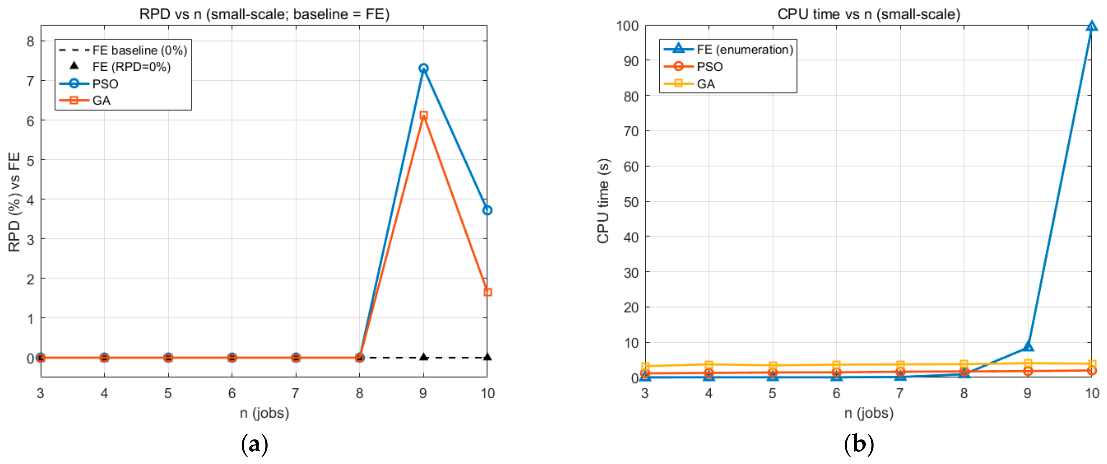
To verify the correctness of the proposed model and algorithms, small-scale instances with 3–10 jobs were tested. Decoder-space full enumeration provides the optimum within the decoded priority-sequence representation for these cases. For n ≤ 8, both GA and PSO attain the decoder-space enumeration optimum, confirming the implementation on small instances. For n = 9 and n = 10, the search space is already much larger, and the metaheuristics do not always attain the decoder-space optimum within the fixed budget. This does not imply that the methods fail on larger instances; rather, it shows the expected loss of exact optimality guarantees as the permutation space grows and motivates reporting deviations, repeated runs, and statistical comparisons in the subsequent experiments. The decoder-space enumeration and metaheuristic results for instances with n=3–10 are summarized in

Table 5. Small-scale results (n = 3–10).

n	Objective Function Values (Bold Numbers Show the Optimal)			Computational Times (s)
	FE	PSO	GA	FE	PSO	GA
3	249.57	249.57	249.57	0.0232	1.1648	3.2258
4	366.15	366.15	366.15	0.0503	1.2868	3.7114
5	526.22	526.22	526.22	0.0450	1.4211	3.4542
6	975.64	975.64	975.64	0.0442	1.4590	3.6233
7	1406.68	1406.68	1406.68	0.1357	1.6247	3.7142
8	1524.14	1524.14	1524.14	0.9166	1.7118	3.7652
9	1694.31	1818.11	1798.05	8.4805	1.8045	4.0598
10	1943.91	2016.26	1976.24	99.3930	1.9955	3.8995

Note: Bold values in the FE objective column denote the decoder-space enumeration optimum. Bold values in the computational-time columns denote the shortest runtime for each problem size.

.

To compare algorithms on each test instance l, we report the relative percentage deviation from the best-found value:

$${RPD}_{A,l}=\left({\displaystyle \frac{T{C}_l^A-T{C}_l^{Best}}{T{C}_l^{Best}}}\right)\times 100\%$$

(14)

where $T{C}_l^A$ is the total cost of algorithm A on instance l and $T{C}_l^{Best}$ is the best reference value for that instance. For n ≤ 10, $T{C}_l^{Best}$ = $T{C}_l^{FE}$ (enumeration optimum) is the decoder-space enumeration optimum. For n ≥ 20, it is the best-known value obtained across algorithms and runs.

Two percentage measures are used to avoid ambiguity. RPD measures deviation from the best reference value, while Gain measures the relative improvement of GA over PSO on the same instance.

$${\mathrm{G}\mathrm{a}\mathrm{i}\mathrm{n}}_{\mathrm{G}\mathrm{A}\leftarrow \mathrm{P}\mathrm{S}\mathrm{O},\mathrm{l}}=100\times {\displaystyle \frac{T{C}_l^{PSO}-T{C}_l^{\mathrm{G}\mathrm{A}}}{T{C}_l^{\mathrm{P}\mathrm{S}\mathrm{O}}}}(\%)$$

(15)

RPD is non-negative and equals 0% when an algorithm reaches the best-known or optimal value. Positive values indicate that GA gives a lower total cost than PSO on that instance.

Figure 1 compares GA and PSO in terms of RPD (in Figure 1a) and CPU time (in Figure 1b) on small instances. The results indicate a quality-time trade-off under the tested budget: GA tends to stay closer to the decoder-space optimum for the larger small cases, whereas PSO converges faster.

The small-scale trials confirm the implementation and show how quickly decoder-space exact optimality becomes difficult as n increases. GA benefits from crossover, mutation, elitism, and local search, while PSO benefits from rapid swarm convergence. Under the fixed budget, GA generally provides better cost accuracy, whereas PSO requires less CPU time. This supports the subsequent medium- and large-scale experiments, where decoder-space enumeration is no longer practical.

3.3. Medium- and Large-Scale Performance

To assess scalability, experiments were extended to instances with 20–70 jobs. The comparison between GA and PSO is reported in terms of total cost, CPU time, convergence, robustness, and cost composition.

Table 6. Medium/large-scale results.

Number of Jobs	PSO			GA
	CPU	Value	RPD (%)	CPU	Value	Gain vs. PSO (%)
20	2.8490	5733.08	1.0589	4.8348	5673.01	1.0478
30	3.9657	11,097.31	28.9231	6.1258	8607.70	22.4344
40	4.9496	16,887.59	34.2917	7.0437	12,575.30	25.5353
50	6.1203	25,834.58	30.2457	8.1244	19,835.26	23.2221
60	7.4519	43,633.58	47.4446	9.5726	29,593.20	32.1779
70	9.2828	73,055.73	63.9357	11.9096	44,563.65	39.0005

Note: PSO RPD (%) is computed relative to the best-known total cost in each row. GA gain vs. PSO (%) is computed relative to the PSO total cost in the same row. The two percentages have different denominators and are reported for different interpretive purposes.

summarizes the CPU time, objective values, PSO RPD from the best-known value, and GA gain over PSO. The results indicate a quality-time trade-off under the adopted settings: GA obtains lower total costs in these instances, whereas PSO requires a shorter CPU time.

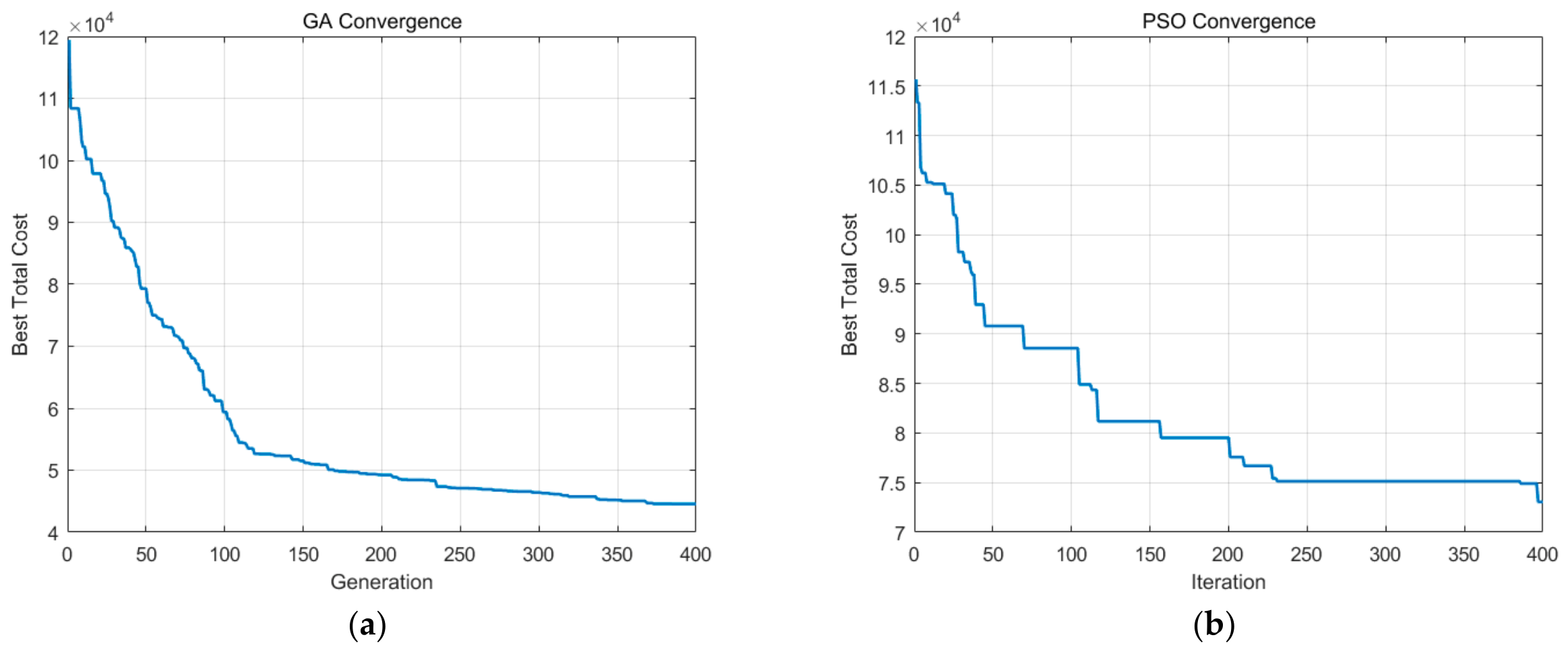
Figure 2 shows representative convergence profiles under the same computational budget. GA reduces the objective rapidly during early exploration and then improves gradually, whereas PSO shows staircase-like changes with plateau periods. These profiles are consistent with the aggregate results: GA tends to provide a lower final cost, while PSO is faster but more prone to stagnation under the tested settings.

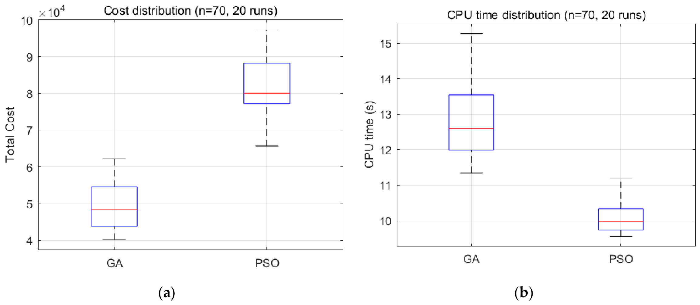
For n = 70, 20 independent runs were conducted.

Table 7. Statistical summary of GA and PSO performance on medium/large-scale instances (n = 70).

n	Algorithm	Mean Cost	Std Cost	CV (%)	Mean CPU (s)	Std CPU (s)	Mean RPD (%)	Std RPD (%)
70	GA	49,455.46	7129.51	14.42	12.92	1.21	0.00	0.00
70	PSO	81,614.94	7988.11	9.79	10.07	0.44	66.48	14.96

CV = 100 × Std/Mean.

and Figure 3 report the mean, standard deviation, and coefficient of variation (CV, %) in total cost and CPU time. RPD (%) is computed for each seed relative to the best-known value obtained by GA or PSO under the same instance and seed setting.

To assess robustness under stochastic effects, each algorithm was executed 20 independent times on the large-scale instance with n = 70, using different random seeds but identical parameter settings and computational budgets. RPD (%) was computed per seed against the best-known value between GA and PSO for that seed. Table 7 summarizes the mean, standard deviation, and coefficient of variation (CV) in the total cost and CPU time, and Figure 3 reports the corresponding boxplots.

For the n = 70 instance, PSO requires less CPU time, whereas GA achieves a substantially lower mean total cost. Figure 3a shows that the GA cost distribution lies below the PSO distribution, while Figure 3b confirms that PSO has a lower median runtime and a narrower runtime spread. These results indicate a quality–time trade-off under the investigated settings: PSO is attractive for rapid screening, whereas GA is preferable when a lower total cost is the primary criterion.

The same quality-time pattern appears in the scalability experiments with n = 30, 50, and 70 jobs.

Table 8. Runtime and absolute expenses.

Alg	n	Energy	Tardiness	Maint.	Total Cost	Runtime (s)
GA	30	802.70	10,430	600	11,832.7	6.3436
PSO	30	803.24	12,200	600	13,603.2	4.0664
GA	50	1252.25	24,050	1000	26,302.2	8.8598
PSO	50	1249.79	34,710	1050	37,009.8	6.3494
GA	70	1772.05	46,280	1400	49,452.0	10.6613
PSO	70	1769.24	79,380	1450	82,599.2	8.6266

Notes: “Maint.” = maintenance cost. Costs keep 1–2 decimals; runtime keeps 4 decimals.

and

Table 9. Cost composition and relative change in PSO vs. GA.

Alg	n	Energy (%)	Tardiness (%)	Maint. (%)	ΔTotal Cost (%)	ΔRuntime (%)
GA	30	6.8	88.1	5.1
PSO	30	5.9	89.7	4.4	+15.0	−35.9
GA	50	4.8	91.4	3.8
PSO	50	3.4	93.8	2.8	+40.7	−28.3
GA	70	3.6	93.6	2.8
PSO	70	2.1	96.1	1.8	+67.0	−19.1

summarize absolute cost, runtime, cost composition, and relative change. Percentages are normalized by the total cost of each row and rounded to 0.1%. For each n, Δ denotes the relative difference between PSO and GA, calculated as (PSO − GA)/GA × 100%; positive values indicate that PSO is higher in cost or runtime, while negative values indicate that PSO is lower. Table 8 and Table 9 show that PSO generally requires less runtime, whereas GA consistently obtains a lower total cost. 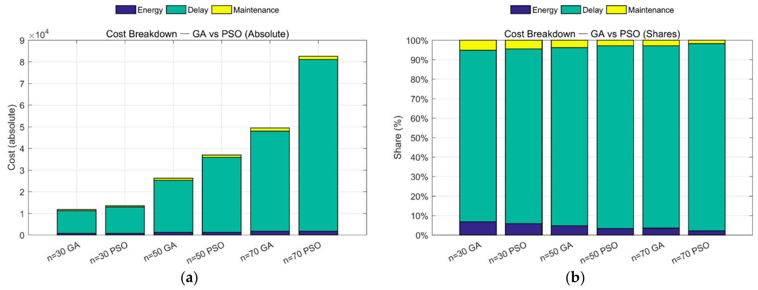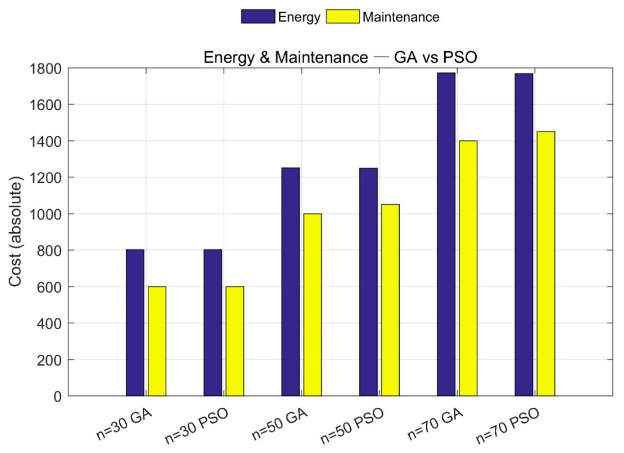Figure 4 and Figure 5 visualize these cost-composition patterns.

Figure 4 and Figure 5 decompose the total cost into energy, tardiness, and fixed-maintenance components. These figures should be interpreted as descriptive cost decomposition rather than as standalone causal proof of an energy–maintenance synergy.

The high share of tardiness costs is mainly due to the due-date generation scheme and the penalty setting γ = 10 MU/min. As n increases while only two machines are available, the same tightness settings create stronger competition for capacity, so lateness penalties dominate total cost. This explains why the tardiness cost exceeds 90% of the total cost in the larger cases, without requiring a separate modeling assumption.

The reliability-dependent energy term still matters because schedules that process many jobs under degraded reliability accumulate higher energy costs and may trigger PM at different times. However, the observed total-cost advantage of GA is primarily associated with its ability to avoid tardiness escalation through better priority sequencing and decoded assignment, rather than with lower energy costs alone.

Accordingly, Figure 5 illustrates how energy and maintenance components differ across algorithms after scheduling decisions have been made. It does not by itself prove a direct causal pathway. The causal mechanism is represented by the model equations and then examined through paired runs, cost decomposition, and sensitivity analysis.

In summary, GA obtains a lower total cost in these experiments mainly by preserving schedule feasibility and limiting tardiness growth, while PSO often offers a shorter runtime and sometimes a lower energy-related cost. The evidence therefore supports a conditional quality–time trade-off under the tested settings.

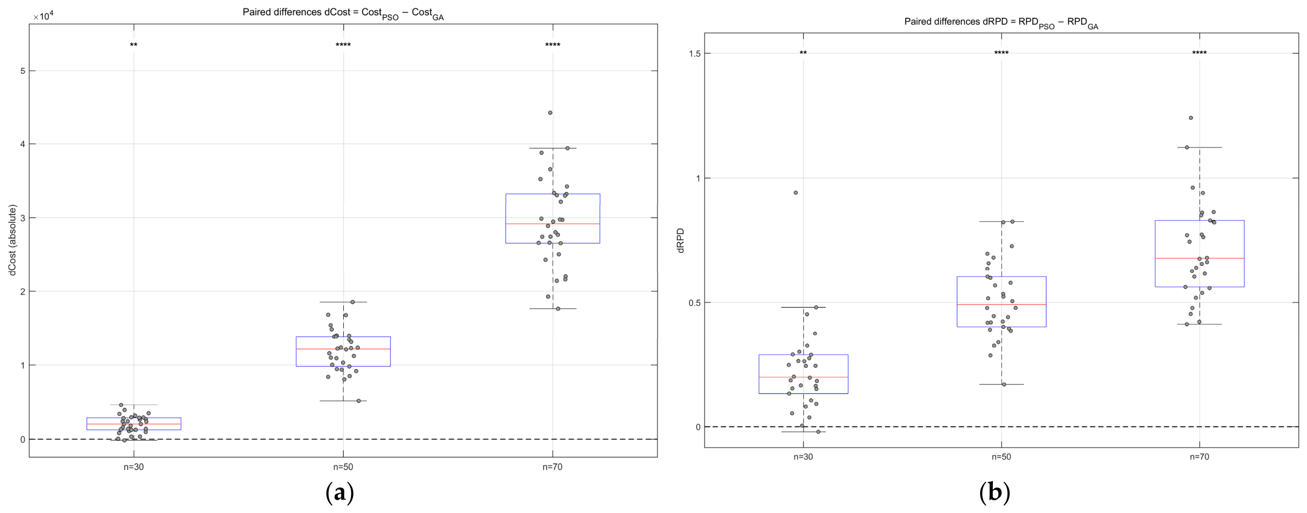
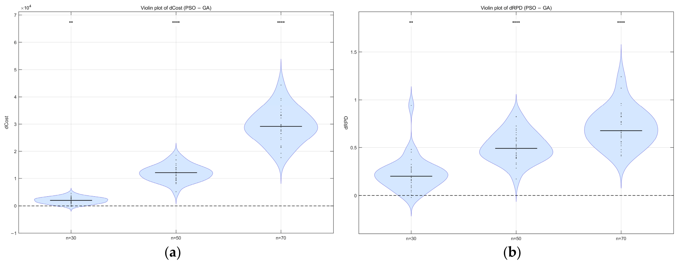
For statistical validation, 30 paired instances were generated for each size n ∈ {30, 50, 70} using matched processing-time and due-date seeds. Both algorithms were run under the same settings, and paired differences were computed so that positive values indicate a higher PSO cost relative to GA. Normality was checked with the Shapiro–Wilk test at α = 0.05. A paired t-test was used when normality was not rejected, and a Wilcoxon signed-rank test was used otherwise. Holm–Bonferroni adjustment controlled family-wise error across sizes and metrics. Effect sizes were reported as Hedge’s $g$ for paired t-tests and rank-biserial correlation for Wilcoxon tests. Boxplots and violin plots complement the p-values by showing the distribution of paired differences.

Total cost (paired t-test):

$${n=30:P}_{h_{0}lm}=0.00267,g=1.336\left(large\right);$$

$${n=50:P}_{h_{0}lm}=4.06{\times 10}^{-7},g=4.643\left(very large\right);$$

$${n=70:P}_{h_{0}lm}=1.52{\times 10}^{-6},g=3.904\left(very large\right);$$

RPD (Wilcoxon for n = 30; paired t otherwise):

$${n=30:P}_{h_{0}lm}=0.00267,r_{rb}=1000\left(very large, all difference aligned\right);$$

$${n=50:P}_{h_{0}lm}=6.61{\times 10}^{-6},g=3.201\left(very large\right);$$

$${n=70:P}_{h_{0}lm}=1.06{\times 10}^{-5},g=2.922\left(very large\right);$$

Table 10. Summary of paired tests and effect sizes (PSO − GA).

n	Metric	Test	p-Value	Holm-Adjusted p	Effect Size
30	Total cost	Paired t	0.001335	0.00267	g = 1.336
30	RPD	Wilcoxon	0.001953	0.00267	$r_{rb}=1.000$
50	Total cost	Paired t	6.769 × 10−8	4.601 × 10−7	g = 4.643
50	RPD	Paired t	1.653 × 10−6	6.613 × 10−6	g = 3.201
70	Total cost	Paired t	3.045 × 10−7	1.522 × 10−6	g = 3.904
70	RPD	Paired t	3.546 × 10−6	1.046 × 10−5	g = 2.922

Note: g denotes Hedges’ $g$ for paired t-tests, and $r_{rb}$ denotes rank-biserial correlation for Wilcoxon signed-rank tests. (Interpretation thresholds: Hedges’ $g$ ≈ 0.2 small, 0.5 medium, 0.8 large; $\left|r_{rb}\right|$ ≈ 0.147 small, 0.33 medium, 0.474 large.)

shows that, under the selected experimental parameters, GA achieves substantially lower total cost than PSO on this instance set, and that the cost difference increases with instance size.

The statistical results are consistent with the descriptive cost decomposition. On the tested paired instances, GA more often produces schedules with lower total cost, and the magnitude of this difference grows with size. This should be interpreted as practical evidence under the selected model, data-generation scheme, and computational budget, not as a universal ranking of GA and PSO.

For each instance size, each box aggregates 30 paired observations; dots represent individual pairings, and the dashed line indicates zero difference. Significance stars above each group reflect Holm–Bonferroni adjusted levels. Positive medians across all sizes indicate that PSO incurs a higher cost than GA. As shown in Figure 6a, the distributions lie above zero and widen with size, indicating that PSO’s relative cost disadvantage increases as n grows.

Figure 7a shows violin plots of total-cost differences (PSO−GA). Shaded density shows the distribution; black bars denote medians. The mass is consistently above zero, with much broader and higher densities at n = 50, 70, mirroring the very large Hedges’ g values.

Medians and densities are again above zero and expand with size, confirming a scale-amplified relative gap. Across m = 30 paired instances for each size, these paired distributions further support the conditional cost-quality advantage of GA under the tested model, instance-generation scheme, and computational budget.

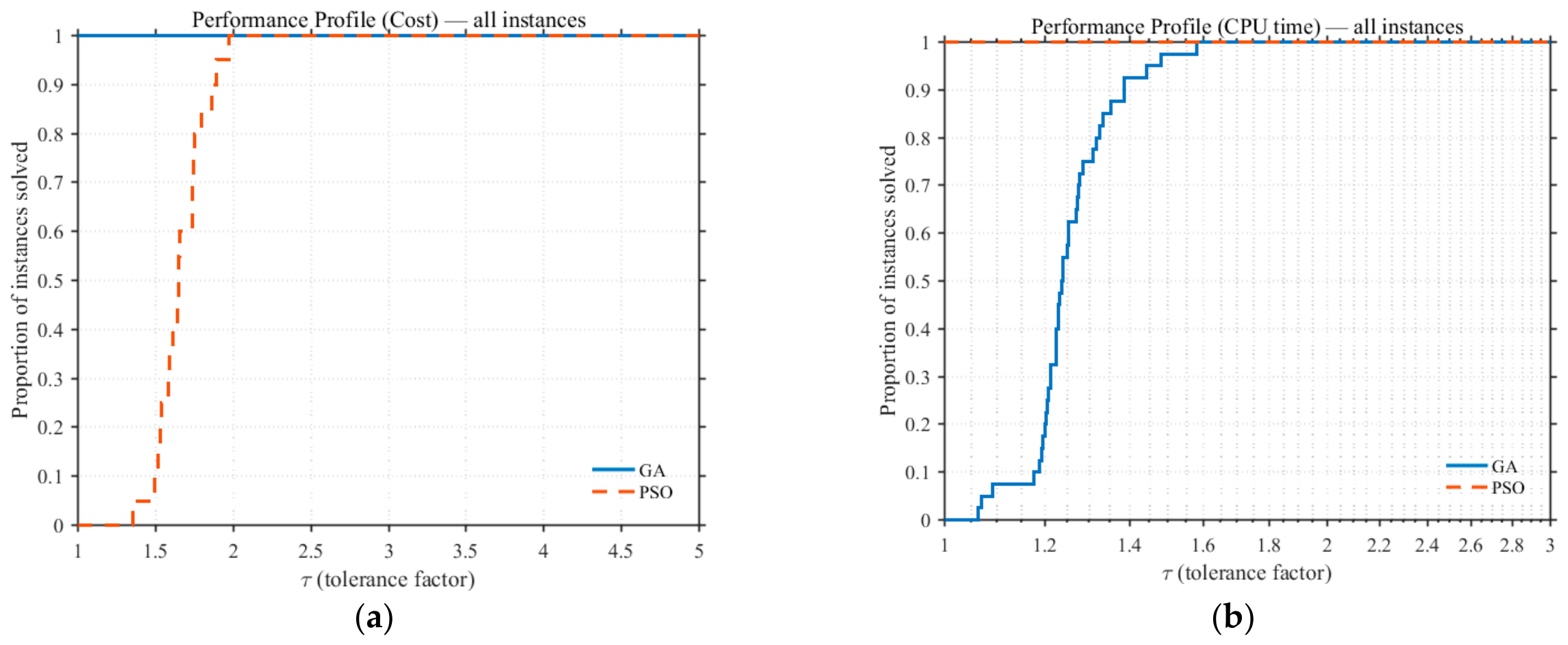
To compare robustness across instances, we use the Dolan–Moré performance profile. For each instance j, let $m_{a,j}$ (smaller is better) denote the performance of algorithm a. We use the total cost (energy + tardiness + maintenance) as a measure of solution quality and plot a separate profile for CPU time. The per-instance ratio is

$$r_{a,j}={\displaystyle \frac{m_{a,j}}{\underset{b}{min} m_{b,j}}}(\ge 1),$$

(16)

and the cumulative distribution for tolerance τ ≥ 1 is

$${\rho }_a(\tau )={\displaystyle \frac{1}{N_{\mathrm{e}\mathrm{f}\mathrm{f}}}}|\{j:r_{a,j}\le \tau \}|,$$

(17)

The intercept ${\rho }_a$ (1) gives the fraction of best (or tied-best) cases; larger τ quantifies how often an algorithm attains near-optimal solutions. For stability and interpretability, profiles are drawn on cost and CPU time; RPD% is summarized in the appendix via boxplots and Wilcoxon/Cliff’s-delta statistics.

Figure 8a shows that GA reaches the best-known total cost more frequently than PSO under the tested settings, whereas PSO requires a larger tolerance factor to cover all instances. Figure 8b shows the opposite pattern for CPU time: PSO reaches the best-known runtime more frequently, while GA requires a larger tolerance factor. Therefore, the performance profiles indicate a clear quality–time trade-off rather than an unconditional dominance relationship.

3.4. Sensitivity Analyses

3.4.1. Model-Parameter Sensitivity

We quantify the influence of six factors on total cost across two metaheuristics, PSO and GA, using a one-at-a-time (OAT) sensitivity study. The factors are due-date tightness T, due-date dispersion D, reliability decay rate λ, energy coefficient α, preventive-maintenance (PM) trigger threshold $r^{th}$, and tardiness penalty γ. The total cost is decomposed into Energy + Tardiness + Maintenance; PM occurrences are also recorded.

Baseline (shared by both algorithms): T = 0.70, D = 0.40, λ = 0.010, α = 0.50, $r^{th}$ = 0.70, γ = 10. Baseline totals: PSO 73,055.7 and GA 44,563.6.

Factor levels are T ∈ {0.50, 0.70, 0.90}, D ∈ {0.20, 0.40, 0.60}, λ ∈ {0.005, 0.010, 0.020}, α ∈ {0.30, 0.50, 0.80}, $r^{th}$ ∈ {0.60, 0.70, 0.90}, and γ ∈ {5, 10, 20}.

Table 11. Baseline vector and OAT perturbation levels.

Parameter	Baseline	Levels
T	0.7	0.5, 0.7, 0.9
D	0.4	0.2, 0.4, 0.6
λ	0.01	0.005, 0.01, 0.02
α	0.5	0.3, 0.5, 0.8
$r^{th}$	0.7	0.6, 0.7, 0.9
γ	10.0	5, 10, 20

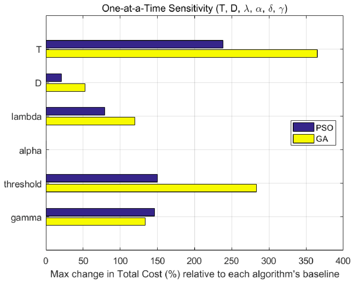
reports the baseline vector and OAT levels, while Figure 9 summarizes factor influence with a tornado chart. This part evaluates model-parameter sensitivity. A separate algorithm-budget sensitivity experiment is reported in Section 3.4.2. Formal Pareto-front construction remains outside the present scalarized single-objective formulation and is discussed as a future extension.

$$\Delta \%=100\times {\displaystyle \frac{max\left(\mathrm{T}\mathrm{o}\mathrm{t}\mathrm{a}\mathrm{l}\right)-min\left(\mathrm{T}\mathrm{o}\mathrm{t}\mathrm{a}\mathrm{l}\right)}{\mathrm{Baseline} \mathrm{Total}}}.$$

(18)

Metric (tornado bars): Δ% is computed as above.

Figure 9 shows that the total cost is most sensitive to due-date tightness T and PM trigger threshold $r^{th}$, whereas the energy coefficient α has a smaller effect under the tested levels. From a managerial perspective, due-date tightness T and the PM trigger threshold $r^{th}$ are the two main controllable levers. Tighter due dates increase tardiness pressure, whereas a higher, more conservative PM trigger threshold can increase maintenance frequency and disrupt machine synchronization. These results suggest that due-date policy and PM trigger threshold selection should be calibrated jointly rather than independently.

The detailed OAT sensitivity results for PSO are presented in Table 12.

Table 12. OAT sensitivity summary for PSO.

Param	Base Lvl	Base Total	Min (Lvl, Total)	Max (Lvl, Total)	Δ% (vs. Base)	Dominant @Max	ΔE @Max	ΔTardiness @Max	ΔM @Max	ΔPM
T	0.700	73,055.7	0.500, 16,352.7	0.900, 190,696.0	238.6	Tardiness	0.3	117,690.0	−50.0	−1
$r^{th}$	0.700	73,055.7	0.600, 64,185.9	0.900, 173,633.0	149.8	Tardiness	57.2	98,270.0	2250.0	45
γ	10.000	73,055.7	5.000, 37,920.7	20.000, 145,005.0	146.6	Tardiness	−0.9	71,950.0	0.0	0
λ	0.010	73,055.7	0.005, 59,013.7	0.020, 116,605.0	78.8	Tardiness	39.6	42,610.0	900.0	18
D	0.400	73,055.7	0.400, 73,055.7	0.600, 88,220.8	20.8	Tardiness	−4.9	15,120.0	50.0	1
α	0.500	73,055.7	0.300, 73,022.6	0.800, 73,105.4	0.1	Energy	49.6	0.0	0.0	0

Δ% = (max − min)/baseline × 100. Totals share the same unit as the model. Values rounded; thousands separated. The results indicate moderate variations, with Δ% for T reaching 238% and the $r^{th}$ factor reaching about 149%. For GA, Table 13 reports the corresponding sensitivity results.

Table 12. OAT sensitivity summary for PSO.

Param	Base Lvl	Base Total	Min (Lvl, Total)	Max (Lvl, Total)	Δ% (vs. Base)	Dominant @Max	ΔE @Max	ΔTardiness @Max	ΔM @Max	ΔPM
T	0.700	73,055.7	0.500, 16,352.7	0.900, 190,696.0	238.6	Tardiness	0.3	117,690.0	−50.0	−1
$r^{th}$	0.700	73,055.7	0.600, 64,185.9	0.900, 173,633.0	149.8	Tardiness	57.2	98,270.0	2250.0	45
γ	10.000	73,055.7	5.000, 37,920.7	20.000, 145,005.0	146.6	Tardiness	−0.9	71,950.0	0.0	0
λ	0.010	73,055.7	0.005, 59,013.7	0.020, 116,605.0	78.8	Tardiness	39.6	42,610.0	900.0	18
D	0.400	73,055.7	0.400, 73,055.7	0.600, 88,220.8	20.8	Tardiness	−4.9	15,120.0	50.0	1
α	0.500	73,055.7	0.300, 73,022.6	0.800, 73,105.4	0.1	Energy	49.6	0.0	0.0	0

Δ% = (max − min)/baseline × 100. Totals share the same unit as the model. Values rounded; thousands separated. The results indicate moderate variations, with Δ% for T reaching 238% and the $r^{th}$ factor reaching about 149%. For GA, Table 13 reports the corresponding sensitivity results.

Table 13. OAT sensitivity summary for GA.

Param	Base Lvl	Base Total	Min (Lvl, Total)	Max (Lvl, Total)	Δ% (vs. Base)	Dominant @Max	ΔE @Max	ΔTardiness @Max	ΔM @Max	ΔPM
T	0.700	44,563.6	0.500, 2682.5	0.900, 165,207.0	364.7	Tardiness	3.5	120,590.0	50.0	1
$r^{th}$	0.700	44,563.6	0.600, 35,420.7	0.900, 161,542.0	283.0	Tardiness	58.6	114,570.0	2350.0	47
γ	10.000	44,563.6	5.000, 27,159.5	20.000, 86,815.4	133.9	Tardiness	1.7	42,200.0	50.0	1
λ	0.010	44,563.6	0.005, 28,423.1	0.020, 81,762.6	119.7	Tardiness	38.9	36,310.0	850.0	17
D	0.400	44,563.6	0.600, 41,804.6	0.200, 65,396.5	52.9	Tardiness	2.8	20,780.0	50.0	1
α	0.500	44,563.6	0.300, 44,529.0	0.800, 44,615.6	0.2	Energy	52.0	0.0	0.0	0

Δ% is equal to (max − min)/baseline × 100. The model and totals have the same unit. Thousands separated; values rounded. Here, the differences are more noticeable: the $r^{th}$ factor surpasses 280% and Δ% for T reaches 360%, highlighting GA’s greater sensitivity to parameter perturbations.

Table 13. OAT sensitivity summary for GA.

Param	Base Lvl	Base Total	Min (Lvl, Total)	Max (Lvl, Total)	Δ% (vs. Base)	Dominant @Max	ΔE @Max	ΔTardiness @Max	ΔM @Max	ΔPM
T	0.700	44,563.6	0.500, 2682.5	0.900, 165,207.0	364.7	Tardiness	3.5	120,590.0	50.0	1
$r^{th}$	0.700	44,563.6	0.600, 35,420.7	0.900, 161,542.0	283.0	Tardiness	58.6	114,570.0	2350.0	47
γ	10.000	44,563.6	5.000, 27,159.5	20.000, 86,815.4	133.9	Tardiness	1.7	42,200.0	50.0	1
λ	0.010	44,563.6	0.005, 28,423.1	0.020, 81,762.6	119.7	Tardiness	38.9	36,310.0	850.0	17
D	0.400	44,563.6	0.600, 41,804.6	0.200, 65,396.5	52.9	Tardiness	2.8	20,780.0	50.0	1
α	0.500	44,563.6	0.300, 44,529.0	0.800, 44,615.6	0.2	Energy	52.0	0.0	0.0	0

Δ% is equal to (max − min)/baseline × 100. The model and totals have the same unit. Thousands separated; values rounded. Here, the differences are more noticeable: the $r^{th}$ factor surpasses 280% and Δ% for T reaches 360%, highlighting GA’s greater sensitivity to parameter perturbations.

Both algorithms are highly sensitive to T and $r^{th}$ (PSO: 238.6% and 149.8%; GA: 364.7% and 283.0%). This indicates that due-date tightness and the PM trigger threshold should be calibrated before fine-tuning secondary parameters. Under these perturbations, PSO exhibits lower variability across most parameters except γ, whereas GA yields lower costs in the main paired experiments. The practical implication is not that one algorithm is universally preferable, but that fast PSO runs can be useful for screening while GA is more appropriate when solution quality is prioritized under the tested settings.

3.4.2. Algorithm-Budget Sensitivity

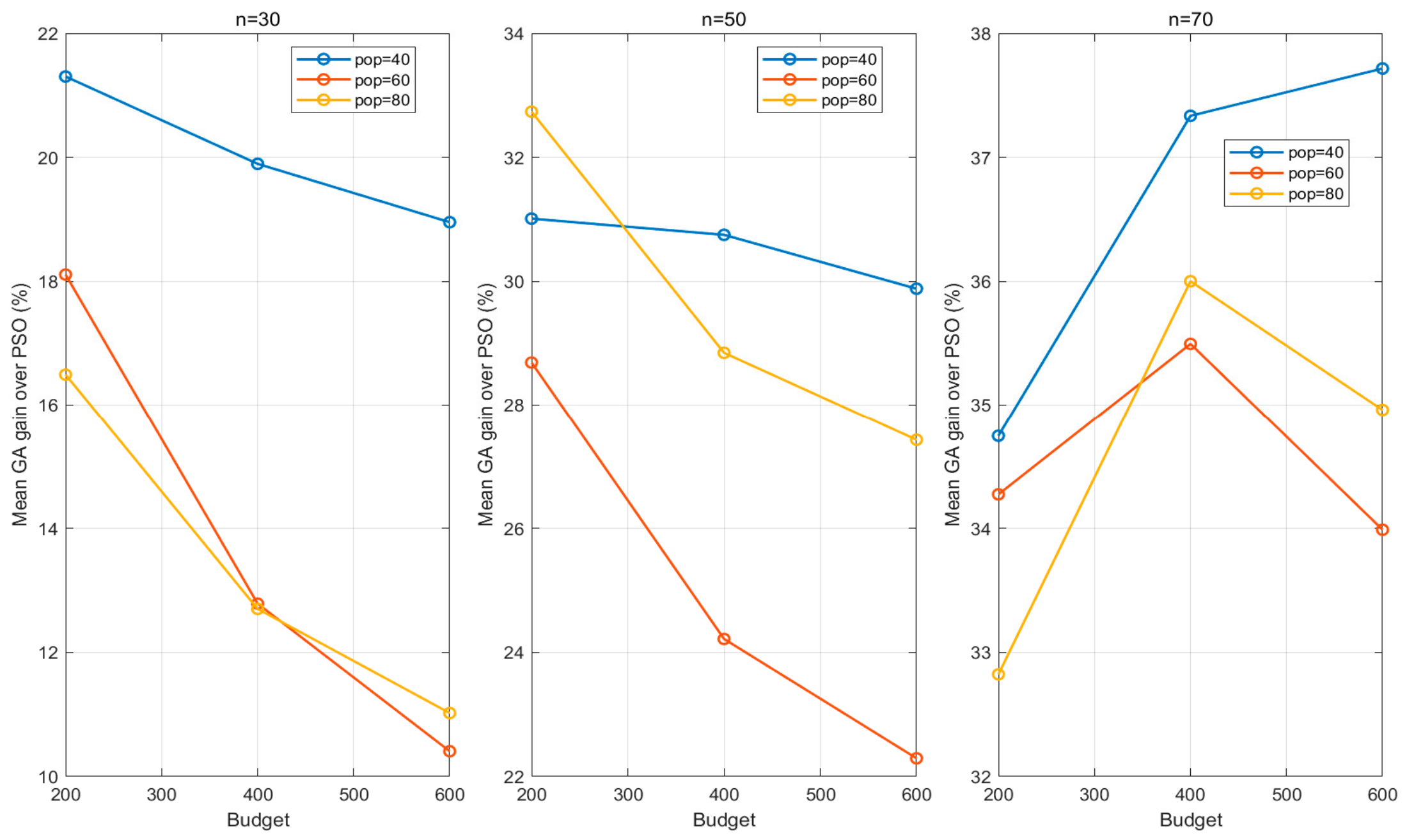
The preceding OAT analysis examines the sensitivity of model parameters. To address the additional concern that the GA-PSO comparison may depend on a single algorithmic budget, we conducted a full algorithm-budget sensitivity experiment. The population or swarm size was varied over {40, 60, 80}, the generation or iteration budget over {200, 400, 600}, and the problem size over n ∈ {30, 50, 70}. For each configuration, ten random seeds were used, producing 270 paired GA-PSO comparisons under the same reliability, energy, PM, and due-date settings as the main application-inspired experiments.

In

Table 14. Algorithm-budget sensitivity summary for GA versus PSO on application-inspired instances.

n	Pairs	GA Wins	PSO Wins	Mean GA Gain (%)	Mean PSO-GA Runtime (s)	Sign-Test p-Value
30	90	85	5	15.74	−1.48	$<1.0\times {10}^{-19}$
50	90	90	0	28.43	−1.59	$<1.0\times {10}^{-26}$
70	90	90	0	35.26	−1.28	$<1.0\times {10}^{-26}$
Overall	270	265	5	26.48	−1.45	$1.24\times {10}^{-71}$

, a positive gain indicates that GA produced a lower total cost than PSO, while a negative PSO-GA runtime difference indicates that PSO was faster. The results show that GA achieved a lower total cost in 265 of 270 paired runs, with an average cost reduction of 26.48% relative to PSO. At the original budget setting closest to the main experiments (population/swarm size 60 and budget 400), GA won 9/10, 10/10, and 10/10 paired runs for n = 30, 50, and 70, respectively. These results indicate that the observed GA cost advantage is not an artifact of a single parameter setting.

Figure 10 further shows that the GA advantage remains positive across all tested population/swarm sizes and computational budgets. The magnitude of the gain varies with problem size and budget, but the direction is stable. PSO preserves its runtime advantage in the matched-budget experiments, which supports a quality-time interpretation: GA is preferable when lower scalarized cost is prioritized, whereas PSO is useful for faster screening under the tested settings.

3.5. Validation on Public Benchmarks

To complement the application-inspired machining instances and improve reproducibility, this section evaluates the proposed framework using public OR-Library weighted tardiness (WT) benchmark instances. The experiment is designed as a reproducibility-oriented model validation rather than as an independent algorithmic benchmark. It tests whether the proposed decoding and cost-evaluation framework remains consistent on public scheduling instances after transparent adaptation. Since the present study considers two identical parallel machines with reliability-dependent energy cost and preventive maintenance, the WT instances cannot be used directly without adjustment. Therefore, processing times and weights are retained, while due dates are scaled to align the tardiness level with the two-machine setting.

This benchmark experiment provides externally validated reproducibility by testing whether the proposed decoding, cost evaluation, and algorithmic comparison remain consistent across community-standard scheduling instances after transparent adaptation to the two-machine reliability-maintenance setting.

• $\beta$: due-date scaling factor, applied as $d_j^{\prime }$ = $\beta {\mathrm{d}}_{\mathit{j}}$.
• TR: tardiness ratio, fraction of late jobs.
• $\epsilon$: alignment tolerance, $\epsilon$ = max{1/n, 0.03} with n $\in$ {40, 50, 100}.
• ${\beta }^{\ast }$: selected due-date scaling factor after calibration.
• ϕ: normalized idle-energy cost rate during PM.

For each instance and each target tardiness level targetTR ∈ {0.2, 0.3, 0.4}, we perform a bisection search over $\beta$ ∈ [0.30, 1.00] to obtain β * such that the reference solver achieves TR(${\beta }^{\ast }$) within tolerance $\epsilon$ on the two-machine model.

For due-date calibration, GA is used as the reference solver for the following reasons:

• Stability and reproducibility: with permutation encoding and repair, TR($\beta$) is monotone and smooth for GA, so bisection reliably meets $\epsilon$;
• Controlled difficulty alignment: once ${\beta }^{\ast }$ is fixed, it is frozen for both solvers so that GA and PSO are evaluated on the same adapted instance. Because the scaling factor is calibrated with GA as the reference solver, this procedure should not be interpreted as algorithm-neutral benchmark construction.

Community baseline: GA is a widely used benchmark heuristic, which facilitates replication. After ${\beta }^{\ast }$ is fixed, GA and PSO are evaluated on the same adapted instance, and E, M, L, Total, and runtime rt are compared in a paired manner.

Solvers:

GA—population 60, 200 generations, tournament selection, Order crossover (OX), swap mutation, elitism.

PSO—swarm 60, 400 iterations, inertia w = 0.72, learning factors c₁ = c₂ = 1.49, random-keys decoding.

Cost parameters follow the main computational setting unless otherwise stated: α = 0.5, λ = 0.002, $r^{th}$ = 0.6, ${\tau }^{PM}$ = 15, $C^{PM}=50$, and ϕ = 0.2.

Pairing: for each (size, targetTR, set), compute the paired total-cost difference $\Delta C_i=C_{total,i}^{PSO}-C_{total,i}^{GA}$ under the same ${\beta }^{\ast }$.

Significance: for each (size, target TR), apply a two-sided sign test to the paired total-cost differences ($\Delta C_i$); where $\Delta C_i=C_{total,i}^{PSO}-C_{total,i}^{GA}$, report wins/losses/pairs and p-values.

To strengthen the computational validation beyond the application-inspired experiments, an adapted OR-Library weighted-tardiness benchmark was introduced as a separate reproducibility-oriented benchmark-validation group.

Table 15. Reproducibility-oriented OR-Library benchmark summary for GA versus PSO under the adopted calibration procedure.

Benchmark Source	Pairs	GA Wins	PSO Wins	Mean GA Improvement (%)	Aggregate Sign-Test p-Value
OR-Library WT40/WT50/WT100 adapted instances	90	86	4	2.96	$4.32\times {10}^{-21}$

summarizes the overall paired comparison between GA and PSO,

Table 16. OR-Library benchmark calibration and target-tardiness alignment for GA.

Size	Target TR	Mean Beta	Achieved TR	Max |TR Error|	Mean Total Cost
WT100	0.2	0.508	0.203	0.020	7886.65
WT100	0.3	0.421	0.301	0.010	9513.43
WT100	0.4	0.332	0.403	0.010	11,688.10
WT40	0.2	0.517	0.203	0.025	2757.34
WT40	0.3	0.421	0.298	0.025	3035.85
WT40	0.4	0.328	0.400	0.000	3408.60
WT50	0.2	0.500	0.200	0.000	3587.09
WT50	0.3	0.411	0.296	0.020	4012.14
WT50	0.4	0.310	0.402	0.020	4650.39

reports the target tardiness-ratio alignment of the adapted instances, and

Table 17. Block-level paired comparison results on adapted OR-Library benchmarks.

Size	Target TR	Pairs	GA Wins	GA Losses	Mean Delta Total (GA-PSO)	Mean Delta Tardiness	Mean Delta Runtime
WT100	0.2	10	10	0	−406.31	−401.12	−4.36
WT100	0.3	10	10	0	−639.17	−623.22	−4.18
WT100	0.4	10	10	0	−774.30	−773.54	−4.43
WT40	0.2	10	10	0	−33.35	−30.40	−1.95
WT40	0.3	10	10	0	−53.31	−48.44	−1.53
WT40	0.4	10	9	1	−45.12	−47.96	−1.85
WT50	0.2	10	9	1	−64.06	−62.32	−2.17
WT50	0.3	10	8	2	−54.39	−51.08	−2.19
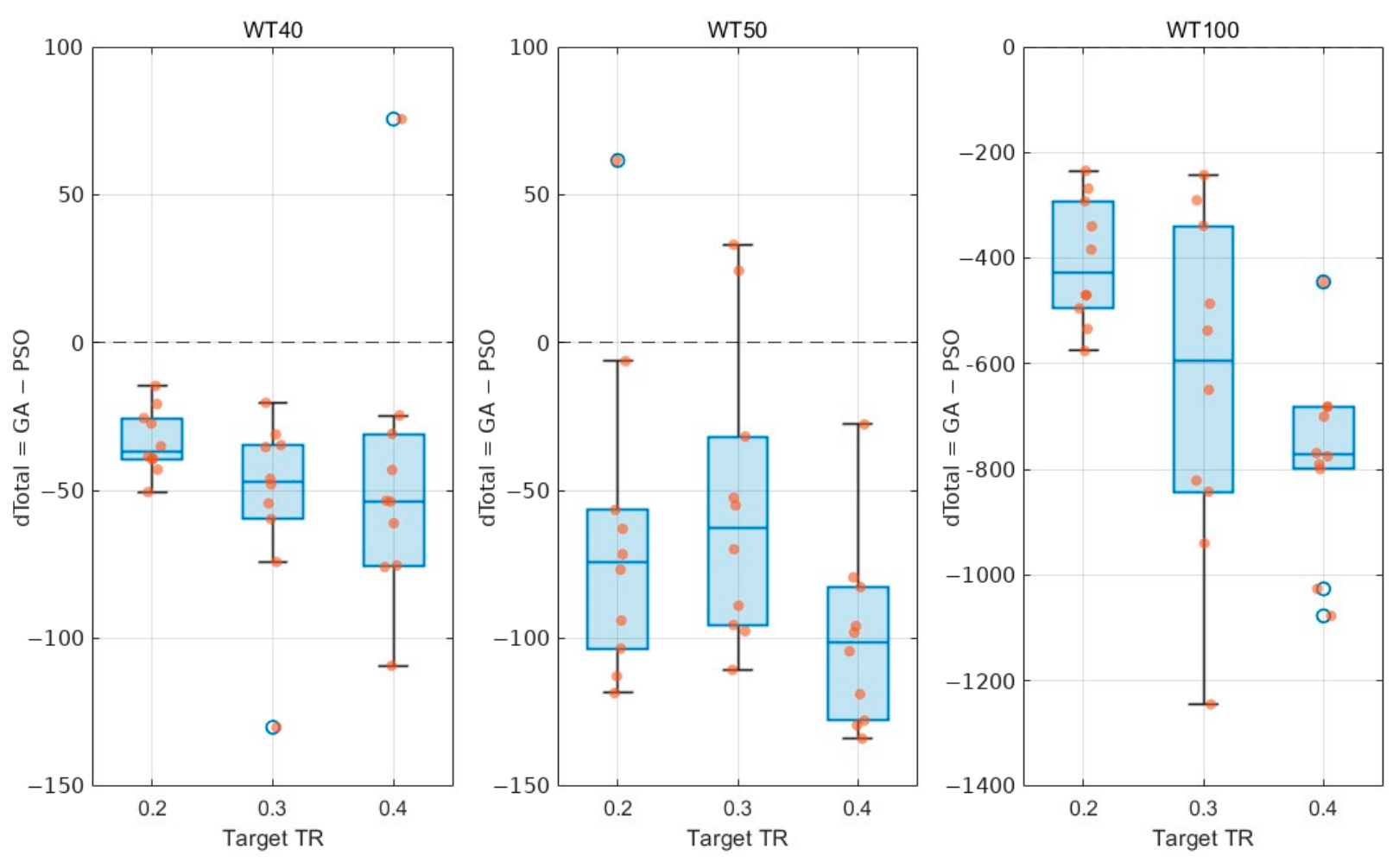
WT50	0.4	10	10	0	−99.72	−101.98	−2.24

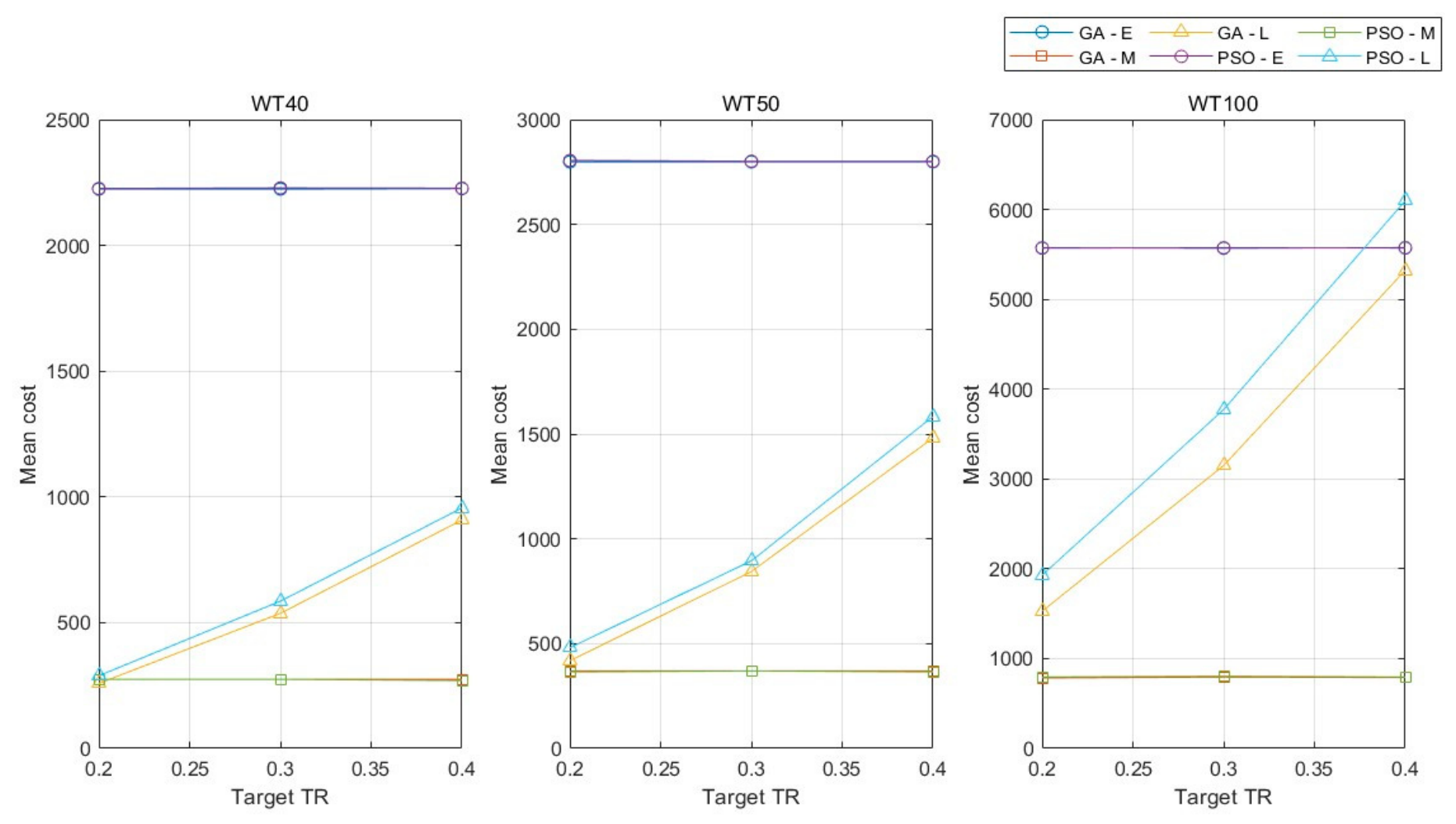
presents the block-level paired results. Across 90 paired benchmark comparisons, GA yielded a lower total cost in 86 cases, with an average improvement of 2.96% over PSO. A two-sided exact sign test indicates that the observed win frequency is statistically significant ($p=4.32\times {10}^{-21}$). Figure 11 and Figure 12 visualize the corresponding cost-component trends and paired total-cost differences.

Runtime results are reported for transparency. However, because the adapted GA and PSO benchmark scripts use different default iteration budgets, runtime is not interpreted as a direct algorithmic efficiency comparison in this benchmark group. Instead, the benchmark results are used primarily as reproducibility-oriented model-validation evidence and conditional cost-quality evidence under the adopted computational settings. Overall, the OR-Library results support the consistency and reproducibility of the proposed framework under adapted public instances. The GA-PSO ranking should be read as conditional on the GA-based calibration procedure, parameter settings, and implementation choices, rather than as an algorithm-neutral proof of GA dominance.

In Table 15, a GA win indicates a paired benchmark case in which GA produced a lower scalarized total cost than PSO. The improvement is computed relative to the PSO total cost. Detailed calibration and block-level comparisons are retained in Table 16 and Table 17.

Table 16 reports the calibration quality of the GA-reference due-date scaling step. The achieved tardiness ratios are close to the target levels within the stated tolerance, so the adapted instances are comparable in tightness before the paired GA-PSO evaluation.

The adapted WT benchmark remains a discrete permutation optimization problem in which sequencing decisions directly determine reliability evolution, PM insertions, energy amplification, and lateness penalties. GA is expected to fit this representation well because permutation encoding preserves feasible job priorities, while OX crossover and swap mutation can recombine promising subsequences without requiring continuous-to-discrete random-key interpretation. However, because due-date scaling was calibrated using GA, the benchmark should be read as reproducibility-oriented support for the framework and conditional cost-quality evidence, not as an algorithm-neutral proof of GA dominance.

Accordingly, the adapted OR-Library experiment is used to check whether the proposed framework behaves consistently under public benchmark data; it is not intended to establish an unconditional solver ranking.

Mean E, M, and L values are plotted against targetTR and grouped by size and solver to illustrate managerial implications under tighter due-date environments.

Key operational lessons are highlighted by the identified trade-offs from a management perspective:

• Tighter due-date environments increase machine utilization pressure. This can raise maintenance costs because faster deterioration triggers more frequent PM, and it can also increase energy costs because machines spend more time in degraded reliability states.
• Lateness cost represents the dominant scheduling trade-off in the tested settings. Earlier processing can reduce tardiness risk, whereas poor sequencing can quickly generate penalties. GA reduces lateness in the studied cases by combining priority sequencing with threshold-based maintenance control.

The managerial implication is that energy management and preventive maintenance should be calibrated jointly under tight delivery requirements. Delaying maintenance may increase short-term throughput, but it can raise downstream costs through higher energy use, reliability losses, and increased downtime risk. The GA schedules demonstrate that proactive PM insertion and improved sequencing can reduce total cost under the tested settings.

4. Conclusions

This study developed a reliability- and energy-aware decision-support framework for production-maintenance scheduling in parallel CNC machining systems. The main contribution is an integrated formulation in which a priority sequence is decoded into machine schedules, reliability evolves endogenously after each job, energy cost depends on the entering reliability state, and preventive maintenance is triggered by the resulting post-job reliability. This structure allows energy, tardiness, and maintenance consequences to be evaluated within one transparent scheduling framework.

The computational study used application-inspired machining instances, decoder-space full enumeration for small cases, repeated stochastic runs, an explicit algorithm-budget sensitivity experiment, and adapted OR-Library benchmark instances. The framework generated feasible schedules and revealed meaningful trade-offs among energy, tardiness, preventive maintenance, and runtime. In the full algorithm-budget sensitivity experiment, GA obtained a lower total cost in 265 of 270 paired application-inspired runs, with an average cost reduction of 26.48% relative to PSO; PSO retained a shorter average runtime under matched budgets. In the adapted public benchmark experiment, GA obtained a lower total cost in 86 of 90 paired comparisons. Together, these findings support a conditional quality–time trade-off under the tested scalarized cost formulation.

Several limitations remain. First, the evidence is based on controlled computational instances rather than confidential high-resolution factory records, so the results should be viewed as reproducible numerical validation and proof of concept. Second, the exponential reliability update is a short-horizon condition index rather than a full lifetime wear model. Third, machine-state transitions such as setup, standby, sleep, and start-up are represented only through normalized coefficients and are not optimized explicitly. Fourth, the current model is single-objective; formal multi-objective Pareto-front analysis, exact-solver or matheuristic comparisons, machine-state power measurements, broader hyperparameter tuning beyond the tested grid, and richer degradation models such as Weibull or gamma-process models are important next extensions.