1. Introduction
Underground coal mine autonomous driving represents a key frontier in industrial safety and efficiency, where real-time trajectory planning and control—core elements for collision avoidance and operational safety—depend critically on continuous, reliable positioning [
1,
2]. Current positioning approaches are shifting from single-sensor to multi-sensor fusion paradigms: GNSS/5G/INS combinations dominate outdoor autonomous driving scenarios, while UWB/5G solutions and kinematic dead reckoning (integrating INS with wheel odometry) are widely applied in GNSS-denied areas [
3]. However, these methods often fail to meet safety-critical requirements in underground coal mines, where harsh conditions amplify the consequences of positioning instability. Advances in LiDAR and camera technologies have established simultaneous localization and mapping (SLAM) as a key enabling technology for high-precision 3D mapping and navigation in complex environments. Yet visual approaches suffer from inherent depth perception limitations and sensitivity to prevalent underground conditions like dust, low light, and high humidity, compromising operational safety continuity. While LiDAR solutions offer better robustness and data accuracy for underground environments, their application requires further optimization for mine-specific challenges [
4].
Underground coal mine environments present unique, safety-centric challenges distinct from conventional autonomous driving scenarios. Kilometer-scale unstructured tunnels—with highly repetitive geometric features, persistently high dust/humidity levels, reduced road adhesion from watering operations, and axial feature deficiencies in long sections—create critical obstacles for safe autonomous driving. Existing research primarily addresses short-term positioning needs, leaving significant technical gaps for long-duration, kilometer-scale navigation [
5]. Key challenges include severe occlusion and multipath effects causing signal-based positioning failures in long tunnels, with incomplete base station coverage leading to intermittent positioning interruptions that increase collision and path deviation risks [
6]; wheel slippage phenomena exacerbated by watering operations that reduce road adhesion, introducing non-Gaussian noise in wheel speed measurements and compromising trajectory tracking accuracy; and the compounding effects of axial feature deficiency and uncompensated cumulative drift, where reduced LiDAR spatial matching constraints combined with long-term navigation drift produce significant positioning deviations that compromise operational safety and continuity [
4].
To overcome these challenges above—including signal obstruction in confined tunnels, non-Gaussian disturbances during wheel slippage, and geometric degradation undermining LiDAR constraints—this work makes four key contributions:
- 1
Onboard-sensor-only self-contained localization for full-scenario coverage: A multi-sensor integration strategy (fusing LiDAR, IMU, wheel speed, and steering angle) is proposed to eliminate reliance on external localization signals. This design enables continuous self-contained localization, achieving seamless coverage even in confined or signal-denied tunnel environments.
- 2
Cascaded filtering architecture for cross-condition localization robustness: A dedicated cascaded filtering mechanism is embedded into the localization system, with integrated anti-slip and anti-degradation functional modules. This architecture establishes a stable technical foundation for maintaining high-precision localization performance across diverse working conditions.
- 3
Low-adhesion-adapted state estimation with slip compensation: An anti-slip prior estimation approach tailored to mine road characteristics is developed. It fuses kinematic models (derived from wheel speed and steering angle) with IMU data and embeds a targeted wheel slip compensation mechanism to ensure reliable state estimation on low-adhesion surfaces.
- 4
Regularized state update for LiDAR degradation resilience: An anti-degradation estimation strategy for LiDAR constraints is presented. It extracts regularization constraints from point cloud degradation states and embeds them into a recursive Bayesian state estimation framework, effectively stabilizing localization updates in geometrically degraded environments.
The remainder of this paper is structured as follows:
Section 2 briefly covers the related work of this study.
Section 3 details the system architecture and technical implementation of core modules.
Section 4 presents experiments based on simulation and field vehicle data. Finally,
Section 5 summarizes contributions and outlines future research directions.
2. Related Work
In the field of vehicular localization, autonomous localization techniques relying solely on onboard sensors (without external infrastructure support) have become a pivotal research direction, driven by the demand for reliable positioning in complex and unstructured environments. With the limitations of single-sensor systems in robustness and accuracy, the paradigm has gradually shifted toward multi-sensor fusion, in which simultaneous localization and mapping (SLAM) technology stands out as a core enabling approach—its ability to acquire real-time 3D spatial information through sensor data matching makes it widely applicable in scenarios where traditional positioning methods fail. For environments with variable lighting or visual obstruction, LiDAR’s illumination invariance and high-precision distance measurement capabilities have established LiDAR-centric SLAM as a preferred technical route, with research initially focusing on optimizing feature extraction, motion estimation, and loop closure detection to enhance performance in general indoor and outdoor scenes.
However, underground coal mine environments present unique challenges that distinguish them from conventional autonomous driving scenarios, placing higher demands on SLAM-based localization systems and exposing critical gaps in existing research. Kilometer-scale unstructured tunnels are characterized by highly repetitive geometric features, persistently high dust and humidity levels, reduced road adhesion due to regular watering operations, and axial feature deficiencies in long sections—these factors collectively degrade sensor performance and disrupt positioning continuity. Visual SLAM systems, for instance, suffer from depth perception failures under low light and dust interference; while LiDAR-based solutions offer better robustness, they still face issues such as reduced spatial matching constraints under feature degradation, and wheel odometry is prone to non-Gaussian noise from wheel slippage. Existing SLAM studies either focus on general scenes (e.g., urban roads, indoor spaces) without adapting to mine-specific harsh conditions, or only address partial challenges while neglecting long-duration, kilometer-scale navigation stability and anti-slip requirements, leaving significant technical gaps for safety-critical underground mining operations [
4,
5].
Against this background, research on LiDAR-centric SLAM has evolved toward multi-sensor fusion to enhance adaptability, with three main technical branches emerging based on sensor combinations. The first branch focuses on laser-only SLAM, where classic algorithms like LOAM lay the foundation by extracting line and plane features for frame-to-frame motion estimation [
7]; subsequent optimizations such as A-LOAM and Lego-LOAM improve real-time performance and accuracy [
8,
9], while LiTAMIN series algorithms reduce registration points through geometric approximation and optimize loop closure to suppress mismatches [
10,
11]. IMLS-SLAM introduces implicit moving least-squares surfaces for submap matching [
12], and methods like Neighborhood Information Constraint enhance adaptability to rugged terrain [
13], though these laser-only systems still struggle in feature-degraded mine tunnels where LiDAR data reliability drops sharply. The second branch integrates LiDAR with IMU to compensate for LiDAR limitations—algorithms like LIO-SAM (graph optimization-based optimization) and FAST-LIO (error-state Kalman framework-based optimization) leverage IMU’s short-term motion estimation accuracy to enhance robustness [
14,
15], with FAST-LIO2 further improving computational efficiency via ikd-tree real-time balancing [
16]. Adaptations for underground robots have also been explored, such as modified LIO-SAM validated in simulated mines [
17], FAST-LIO2 implemented in coal mine tunnels with artificial landmarks to mitigate feature degradation [
18], and FAST-LIO2 adapted for drone navigation in mining tunnels with cumulative error correction via prior map alignment [
19]. However, these LiDAR-IMU fusion systems face two key limitations in mines: some lack analysis of extreme feature degradation [
17,
19], while others rely on artificial landmarks, reducing generalizability [
18]; additionally, during severe degradation (when LiDAR becomes unreliable), IMU drift accumulates rapidly without effective constraints—though methods like quantifiable degradation metrics to suppress IMU updates have been proposed, they still suffer from substantial estimation errors at high speeds due to the absence of absolute references [
20].
The third branch further incorporates wheel odometry into LiDAR-IMU fusion to add motion constraints, as seen in LIWO-SLAM (factor graph optimization) validated in tunnel environments [
21] and LIW-OAM (bundle adjustment-based fusion) [
22]; related architectures have also been tested on indoor vehicles (via EKF-based fusion of wheel speed, IMU, and LiDAR) [
23] and urban roads (via factor graph optimization) [
24]. Nevertheless, existing LiDAR–IMU–wheel fusion methods are designed for ideal road conditions and lack targeted anti-slip mechanisms—frequent wheel slippage/lockup in mines (caused by explosion-proof water spraying) introduces non-Gaussian noise to wheel measurements, severely compromising localization stability in practical mining operations. Beyond LiDAR–IMU and LiDAR–IMU–wheel fusion, LiDAR–ultrasonic combinations have shown promise for robust localization. Wiseman [
25] proposed an ultrasonic rangefinder for autonomous vehicles, which complements LiDAR’s short-range and low-reflectivity measurement limitations—critical for dusty, irregular underground mine tunnels. Premnath et al. [
26] further validated LiDAR–ultrasonic–wheel encoder fusion, showing enhanced localization in narrow spaces by supplementing LiDAR’s missing environmental constraints, though both studies lack adaptation to mining’s high humidity and kilometer-scale needs.
In summary, while existing multi-sensor fusion-based SLAM research has advanced vehicular autonomous localization, critical limitations persist for safety-critical underground coal mine scenarios. Laser-only SLAM exhibits inherent limitations in feature-degraded long tunnels; LiDAR-IMU fusion methods either lack adaptability to extreme mine conditions, depend on non-generalizable artificial landmarks, or fail to constrain IMU drift effectively under severe LiDAR unreliability. Though LiDAR–IMU–wheel fusion adds motion constraints, its design for ideal road surfaces omits targeted anti-slip mechanisms to mitigate non-Gaussian noise from mine-specific wheel slippage (induced by watering operations). These collective gaps result in inadequate localization stability and continuity for kilometer-scale underground mining navigation—motivating the development of a dedicated localization framework to address these mine-specific challenges comprehensively.
3. Methodology
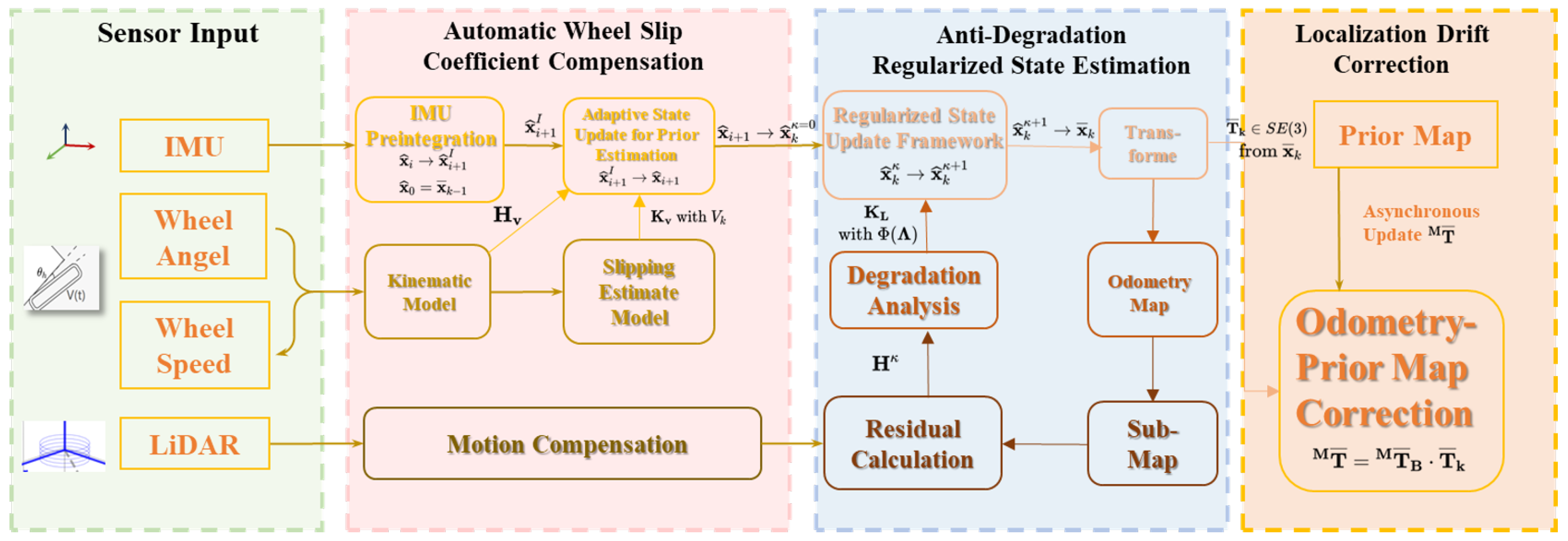
To address large-scale signal-free navigation challenges in underground mines, we pioneer a multi-sensor fusion cascaded filtering SLAM localization system. This innovative architecture aligns with the proposed research contributions and comprises three core components, the system overview as illustrated in
Figure 1:
Multi-sensor fusion cascaded filtering framework: Integrates LiDAR, IMU, wheel speed, and steering angle data to achieve continuous positioning in kilometer-scale lightless tunnels. This framework serves as the core architecture for realizing full-scenario coverage, eliminating reliance on external localization signals and ensuring baseline stability for high-precision localization. Scenario-adapted specialized filtering modules were also used.
An Automatic Wheel Slip Coefficient Compensation Method (
Section 3.1): Tailored for low-adhesion mine road surfaces, this method fuses IMU measurements with vehicle kinematic models derived from wheel speed and steering angle. By extracting non-Gaussian noise features induced by wheel slippage, it constructs an adaptive recursive Bayesian state estimation framework, dynamically adjusting the noise covariance matrix in real time. This mechanism effectively suppresses anomalies caused by slippage, resolving non-Gaussian interference and enhancing system stability in mine environments.
Anti-degradation regularized state estimation module (
Section 3.2): This module addresses geometric degradation in tunnels by constructing observation models based on point-to-plane geometric features between LiDAR point clouds and local maps. It computes Jacobian matrices for the observation model and implements state updates via a nonlinear state estimation framework. To mitigate feature degradation impacts, constraint strength is quantified through residual Jacobian analysis, and a regularization model reflecting system constraint intensity is developed. By embedding feature constraint regularization terms into the state estimation process, updates along weakly constrained directions are explicitly restricted, significantly enhancing robustness in feature-degraded sections.
The state variables involved in the estimation process and their evolution are systematically defined in
Table 1. The overall workflow proceeds as follows: The IMU prior propagation, which yields the predicted state
based on raw inertial data integration, is comprehensively derived and explained in
Section 3.1.1. This prior estimate is subsequently refined using kinematic constraints in
Section 3.1.4, producing the primary filtered state estimate
and its associated error state
. This IMU-Kinematic filtering loop operates iteratively between LiDAR frames.
Upon arrival of the k-th LiDAR point cloud, the framework enters the scan-matching phase. The state from the final IMU–kinematic iteration,
, is designated as the initial value
for LiDAR alignment. The core iterative Kalman filter update, initialized with
, is then executed to optimally fuse the LiDAR observations. The complete derivation and implementation of this process, which culminates in the final optimal state estimate
, are presented in
Section 3.2.3. This cascaded structure ensures computational efficiency and estimation accuracy by decoupling high-frequency propagation from high-precision, low-frequency correction.
Localization drift correction module (
Section 3.3): This module eliminates cumulative errors through prior map constraints, achieving drift-free localization. By matching real-time LiDAR scans with high-precision prior maps, this module performs closed-loop compensation for accumulated localization errors, ensuring sustained high-precision performance during long-range navigation in mining environments.
3.1. Automatic Wheel Slip Coefficient Compensation Method
This section details the construction of a tightly coupled filter for prior pose estimation, which integrates IMU measurements with vehicle kinematic models (derived from wheel speed and steering angle) to implement the Automatic Wheel Slip Coefficient Compensation Method. By analyzing the non-Gaussian disturbance characteristics of wheel speed measurements induced by mine road slippage, we design an adaptive recursive Bayesian state estimation framework for dynamic update. This prior state estimation approach effectively compensates for slip-induced errors, achieving enhanced robustness and improved localization accuracy in low-adhesion underground mine environments.
3.1.1. IMU Integration Model
The IMU evaluates object motion states by measuring three-dimensional acceleration and triaxial angular velocity, providing high accuracy over short durations. We assume rigid connections between the IMU, LiDAR, and vehicle kinematic center, with the IMU (denoted as I) state representing the body localization state. Referencing the definitions of generalized addition ⊞ and subtraction ⊟ from [
27], the discrete pre-integration model is defined as follows, where
i denotes the IMU measurement index:
According to the model definition in [
15], the function
, state
, input
, and noise
are defined as
Variable Definitions:
: Rotation matrix from IMU frame to global frame (SO(3));
: IMU position in global coordinates;
: IMU velocity in global coordinates;
: Gyroscope and accelerometer biases;
: Gravity vector in global coordinates;
: Raw IMU angular velocity and acceleration measurements;
: White noise components.
Since the optimal state estimate after fusing the last (i.e.,
) LiDAR scan is
, when IMU measurement data is received, the system performs forward propagation. Specifically, the state is propagated following Equation (
3) by setting the process noise
to zero.
Using the error state as the update state effectively enhances system linearity and avoids singularities when representing rotational states. The IMU error state forward propagation method is as follows:
During updates, the covariance between true and estimated states is continuously updated:
where
is the noise covariance and
is initialized as follows:
is initialized via gravity vector alignment with high confidence () under static conditions.
assumes origin initialization with high confidence ().
retains moderate uncertainty () for robustness, despite typical stationary assumptions.
is initialized with , reflecting moderate uncertainty in initial bias estimation.
is initialized with , accounting for higher time-varying uncertainty characteristics.
is initialized from normalized accelerometer data with high confidence ().
This initialization strategy balances convergence speed and estimation stability through appropriate parameter weighting in the state estimation process.
The IMU integration-based error state estimate
is computed as
The Jacobians
and
are then calculated as
This completes the discrete-state IMU integration for localization estimation. However, obtaining accurate localization results requires not only high-precision IMU measurements but also reliable estimation of inertial biases and gravity components. Both pose significant challenges in underground mining environments. Specifically, road roughness in mines severely degrades IMU measurement accuracy, while frequent tunnel slopes introduce large errors into gravity direction estimation; these factors collectively amplify sensor measurement deviations.
Owing to error propagation arising from the aforementioned unreliable measurements, IMU integration inevitably leads to the accelerated accumulation of significant localization errors. Consequently, constraints derived from vehicle kinematics (based on wheel speed and steering angle) and LiDAR observations are indispensable for correcting the output of IMU integration—this correction step serves as a critical prerequisite for the subsequent implementation of the Automatic Wheel Slip Coefficient Compensation Method.
3.1.2. Vehicle Kinematic Model
To correct the cumulative errors arising from IMU integration, a vehicle kinematic model is introduced to refine state variables including velocity. The longitudinal velocity of the vehicle (
) is measured via wheel speed sensors, while the yaw rate at the kinematic center is determined by the steering angle (
). The velocity at the kinematic center is decomposed as follows:
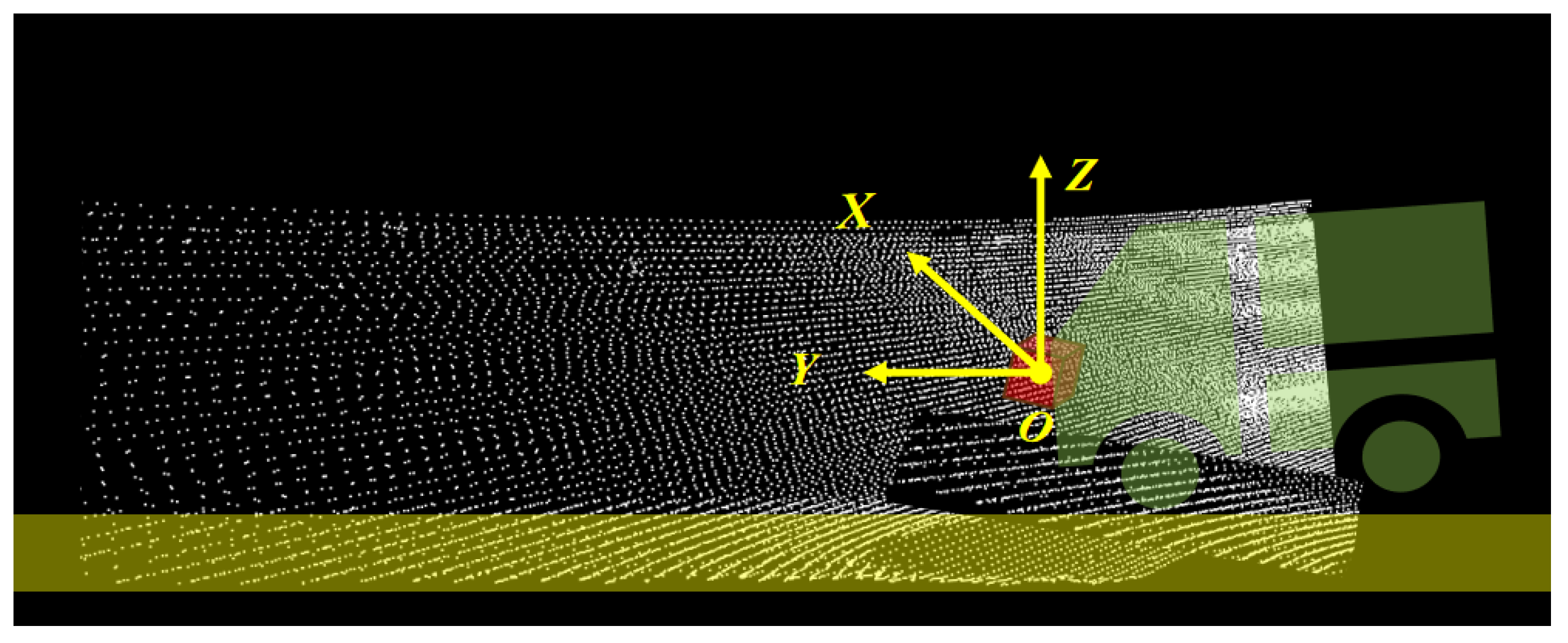
As illustrated in
Figure 2, the IMU is mounted at the front of the vehicle, resulting in a discrepancy between the motion states of the vehicle’s kinematic center (i.e., the rear axle) and the IMU measurement frame. Given the extrinsic parameter
that describes the transformation between the IMU and the rear axle, the relationship between the IMU-integrated states and the kinematically estimated states is formulated as follows:
where
. The observation Jacobian matrix
is computed as
with its components defined as
The observation noise covariance matrix incorporates errors from both wheel speed and steering angle measurements, expressed as
Here, and represent the variances of wheel speed and steering angle, respectively, while accounts for longitudinal vibration during vehicle operation.
This kinematic model enables accurate estimation of horizontal motion and establishes an observation model for velocity states in IMU integration. However, conventional kinematic modeling frameworks only account for inherent measurement noise and lack the capability to filter non-Gaussian slip-induced noise as a critical limitation that compromises localization robustness in underground mine environments where wheel slippage is prevalent. Consequently, an adaptive covariance estimation strategy that accounts for the characteristics of non-Gaussian slip noise is essential to maintain reliable prior state estimation under slippage disturbances, forming a key component of the Automatic Wheel Slip Coefficient Compensation Method.
3.1.3. Adaptive Covariance Estimation
Traditional Kalman filtering assumes Gaussian-distributed sensor measurement errors. For wheel speed measurements, beyond sensor noise, we must account for non-Gaussian errors induced by wheel slippage on wet underground mine surfaces. This paper designs a slip ratio-based adaptive covariance estimation method that dynamically adjusts wheel speed noise covariance according to slippage conditions, mitigating slip impacts. The slip ratio feature is defined as:
Additionally, we consider slip ratio gradient features as follows:
Since longitudinal slippage dominates in most scenarios, we define the comprehensive feature vector for longitudinal slip as follows:
where
represents the sliding window for speed measurements. The weight matrix
updates via
The learning rate
, which controls the update step size, can be tuned based on practical scenarios and has been empirically set to 0.6 in our implementation as this value demonstrates optimal adaptation performance for the current application context. This recursive form implements an exponential moving average, allowing the system to continuously adapt to changing road conditions by emphasizing recent anomaly observations while gradually forgetting distant data. The term
represents the instantaneous outer product of the anomaly vector, serving as a local estimate of the covariance structure at time step
k. To ensure numerical stability and maintain the mathematical integrity of the covariance structure, positive definiteness is enforced through spectral decomposition and reconstruction:
The detailed procedure involves performing eigenvalue decomposition
, where
contains the eigenvectors and
contains the eigenvalues. We compute the modified eigenvalue matrix
with
, where we choose
to be a small positive threshold to eliminate non-positive eigenvalues and reconstruct the positive semi-definite matrix via (
20).
This is followed by a unit trace constraint:
We thus obtain a learning factor and positive-definite weight matrix, enabling adaptive observation noise estimation:
This method achieves wheel speed noise adaptation based on slippage characteristics, which is crucial for subsequent gain calculations.
3.1.4. Adaptive State Update for Prior Estimation
The adaptive state update process follows the error-state recursive Bayesian estimation workflow, with a key modification: fixed noise covariance is replaced by the adaptive noise covariance
(derived in the previous subsection) during velocity fusion gain computation. This modification ensures that the estimation process dynamically responds to slippage-induced non-Gaussian noise. The core update equations are formulated as follows:
where
represents the estimated error state between the kinematically derived states and the IMU-integrated states. The updated states are then obtained via generalized addition and subtraction operations:
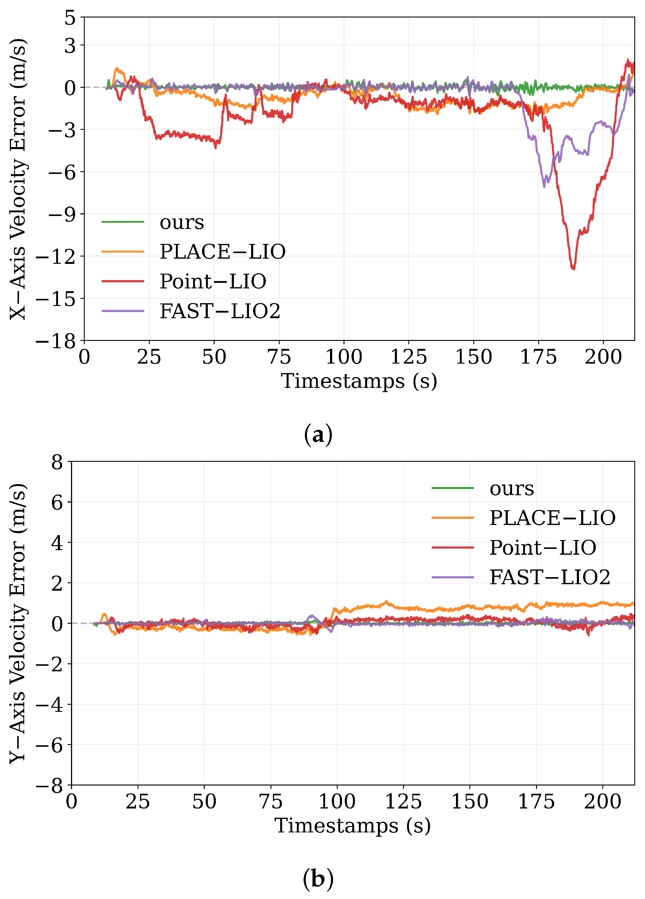
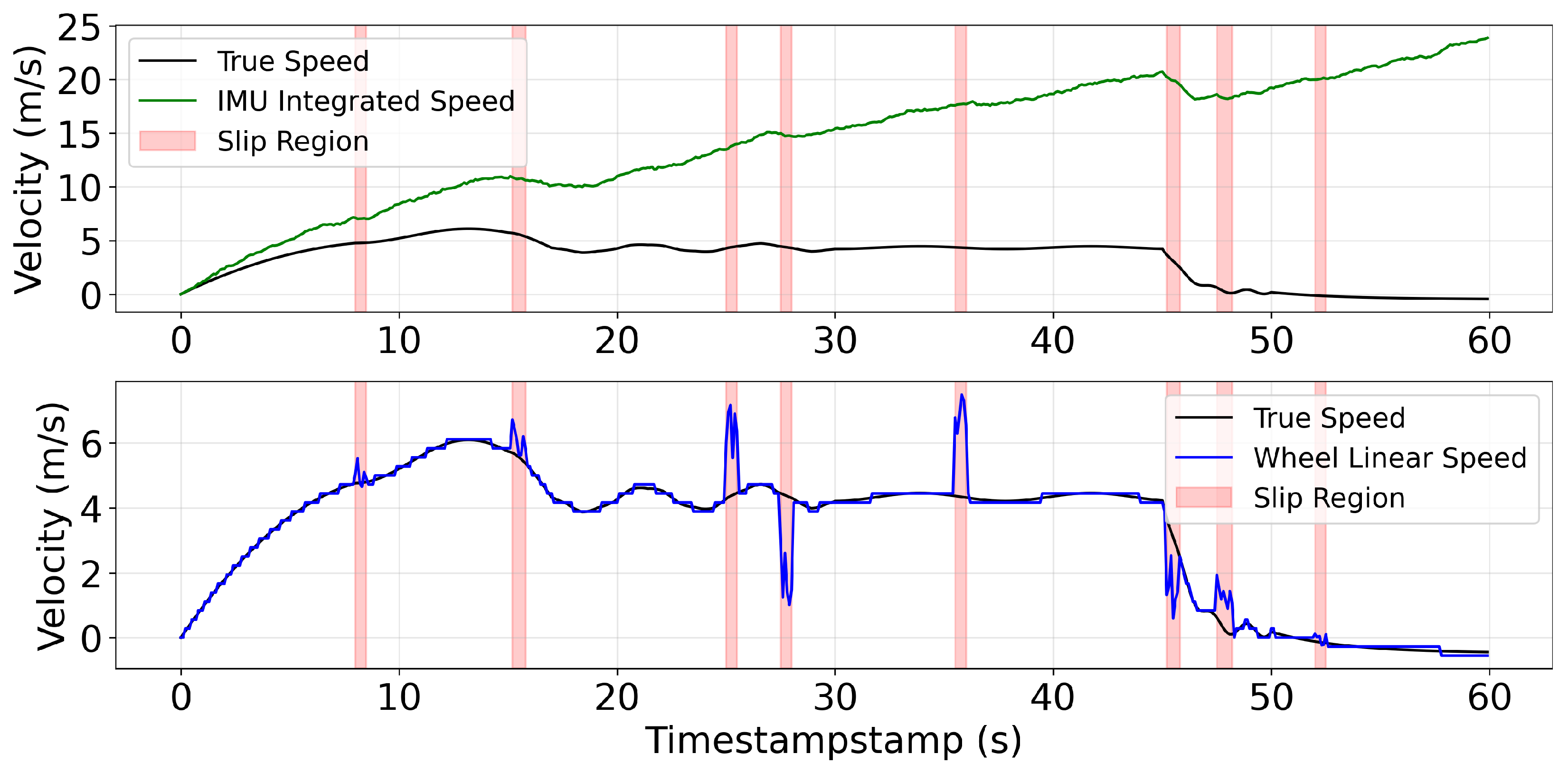
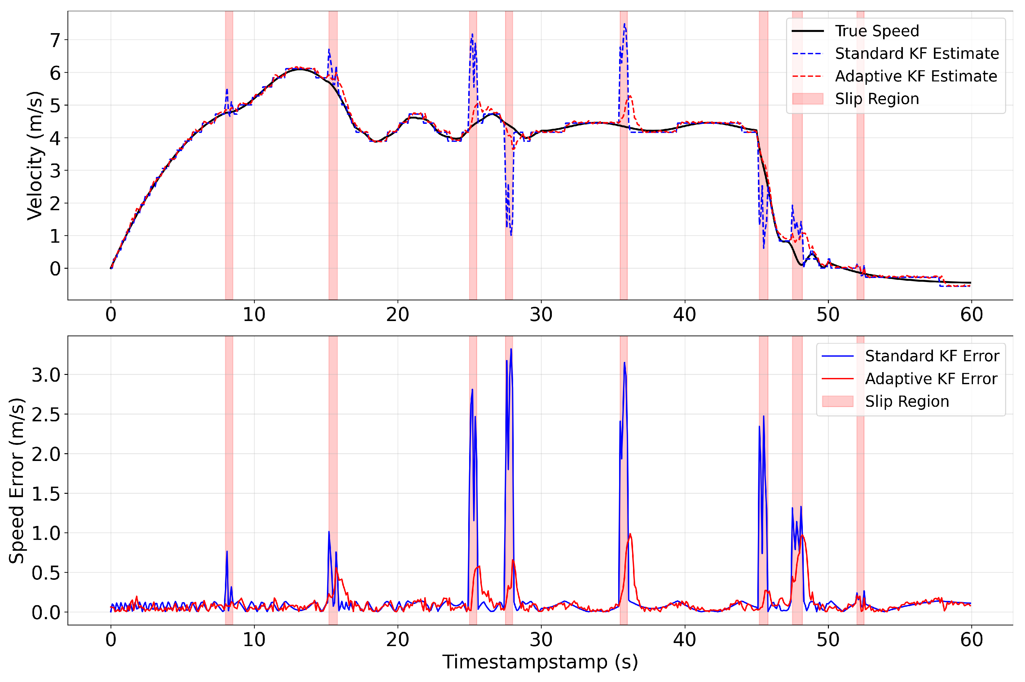
This completes the adaptive state update workflow under dynamically varying noise conditions, thereby facilitating tight coupling between IMU integration and vehicle kinematics. Specifically, dynamic evaluation and adjustment of the wheel speed noise covariance—guided by slippage characteristics—enable the system to maintain robust anti-interference capability in non-Gaussian noise scenarios. Crucially, this capability is foundational to ensuring reliable prior state estimation, a requirement for safe and continuous navigation in underground mine environments. The efficacy of the proposed algorithm is validated through simulation experiments, with detailed results and analysis provided in
Section 4.3.1.
3.2. Anti-Degradation Regularized State Estimation Module
To achieve high-precision pose estimation, posterior refinement of the prior localization state is required, leveraging LiDAR observations as constraints. In feature-degraded underground mining environments (as illustrated in
Figure 3), the majority of LiDAR point clouds are distributed along tunnel roofs, floors, and sidewalls. While these points provide effective constraints in the x and z directions, they exhibit weak constraint capability in the vehicle’s forward direction (y-axis)—a phenomenon that can compromise localization stability. To address this, a degradation-characterizing regularization term is incorporated into the LiDAR observation-based state estimation framework, which restricts posterior state updates along geometrically degenerate directions. This design enhances system robustness under extreme feature degradation scenarios.
3.2.1. LiDAR Observation Model
Following prior state estimation, the prior state
is denoted as
(serving as the input for posterior refinement), and the prior covariance
is denoted as
. To mitigate nonlinear errors in posterior estimation, an iterative update strategy is adopted. Let
represent the state at the
-th iteration, with the initial iteration state set as
. Motion-compensated LiDAR points
are transformed into the global coordinate frame using the following formulation:
where
denotes the estimated transformation from the IMU frame to the global frame at the
-th iteration, and
is the pre-calibrated extrinsic transformation between the LiDAR and IMU frames. Residuals between the transformed LiDAR points
and their nearest corresponding points
on the local map plane are computed as
Here,
, with
representing the unit normal vector of the local map plane at the point
. For the true state
, the LiDAR observation model is defined as
Using the error state definition (where
represents the error between the true state and the estimated state at the
-th iteration), we obtain
A first-order Taylor expansion of the observation model around
yields
In this expression,
denotes the Jacobian matrix of the observation function
evaluated at
, and
represents the observation noise induced by LiDAR measurement errors
, with
being the observed residual at the
-th iteration. The Jacobian matrix
is computed via the chain rule of partial derivatives:
This simplifies to the following form:
where
is the unit normal vector of the plane formed by the nearest neighbors of the LiDAR point
.
3.2.2. Feature Degradation Scenario Analysis
Leveraging the residuals and Jacobian matrices
derived from the LiDAR observation model, maximum a posteriori (MAP) state estimation is achieved by minimizing the residual norm between observed and estimated values. This optimization problem is formulated as
where
and
denote the aggregated residuals of all LiDAR point clouds and their corresponding Jacobian matrices, respectively.
This posterior state estimation problem is solved as a least-squares optimization, whose solution accuracy is critically dependent on the structural characteristics of
. To intuitively illustrate this dependency, the problem can be analogized to finding the closest point to a set of hyperplanes—with a 2D case (locating the point nearest to three lines) used as a representative example, as shown in
Figure 4.
In
Figure 4, black lines represent constraint boundaries and the blue point denotes the optimal estimation solution. Introducing an additional constraint plane
passing through this optimal point does not alter the solution. However, when the constraint plane
is perturbed by
, the solution shifts to the yellow point with a displacement of
. Under strong constraint conditions, as shown in
Figure 4a, such perturbations induce minimal changes in the solution; in contrast, constraint conditions like in
Figure 4b result in significant sensitivity to perturbations, leading to large solution deviations. The optimal solution to the least-squares problem is computed using the left pseudoinverse of
:
where
denotes the left pseudoinverse, defined as follows:
When an additional constraint
(passing through the optimal solution
) is incorporated, the solution remains unchanged, as expressed by
In the presence of a perturbation
applied to the constraint
, the perturbed solution becomes
The displacement
induced by the perturbation
is derived as
The component of this displacement along the direction of the unit vector
(denoted as
) is calculated as
, which simplifies to
The maximum value of
(i.e., the direction of greatest sensitivity to perturbations) is determined by solving the following optimization problem:
Solving this Rayleigh quotient problem reveals that is maximized when is aligned with the eigenvector corresponding to the minimum eigenvalue of . The eigenvalue decomposition of thus enables quantitative evaluation of the system’s disturbance resistance across different directions, providing critical insights for directional suppression of state updates in feature-degraded underground mine environments.
3.2.3. Regularized State Update Framework
Building on the prior state estimation and observation models, posterior state refinement is achieved through an error-state recursive Bayesian estimation framework. The error state (defined as the discrepancy between the true state and the estimated state) satisfies the following relationship:
where the Jacobian matrix
(accounting for state transformation linearization) is formulated as follows:
The operator
follows the definition provided in [
28]. After the
-th iteration, the state covariance matrix is updated via the inverse transformation of
:
Maximum a posteriori (MAP) estimation is employed to fuse prior state information with LiDAR observations, formulated as the following optimization problem that minimizes the weighted residual norm:
Using aggregated terms (where
denotes the stacked Jacobian matrix,
is the block-diagonal observation noise covariance, and
represents the aggregated residuals), the cost function simplifies to
As analyzed in
Section 3.2.2, geometric feature degradation leads to weak observation constraints in specific directions. To address this, a regularization term is introduced to
for directional constraint enhancement. First, eigenvalue decomposition is performed on the Gram matrix of
:
where
(with
representing non-zero eigenvalues) and
denotes the matrix of corresponding eigenvectors. The regularized cost function is then defined as
Here,
is the regularization weight and
is the regularization function, expressed as
In this formulation,
is a diagonal matrix applying eigenvalue-dependent penalties to suppress updates along weakly constrained directions:
where
is a small constant to avoid matrix singularity and
is the eigenvalue threshold distinguishing between strong and weak constraints. For practical implementation,
is typically set to
to ensure numerical stability, while
is empirically chosen as
based on the environmental characteristics. The regularization weight
should typically be set within the range of 0.1 to 10.0 and can be adaptively adjusted based on point cloud density.
The index threshold
corresponds to the positional and orientational degrees of freedom in the state vector. This penalty mechanism inversely weighs the projection of the error state
against eigenvalue magnitude, thereby strongly suppressing state updates along geometrically degenerate directions. Expanding the regularized cost function into a quadratic form yields
To solve the optimization problem, the partial derivative of
with respect to
is computed and set to zero (a necessary condition for the minimum):
Rearranging this equation to solve for
gives
The regularized update gain (analogous to the optimal weight in recursive estimation)
is thus defined as
The state is updated iteratively using the following formulation, which incorporates both the regularized gain and prior state correction:
The iteration terminates when the state change between consecutive iterations falls below a predefined threshold:
. The optimal posterior state and corresponding covariance matrix are then
Finally, LiDAR feature points are projected into the global map coordinate frame using the optimal transformation matrix
:
For navigation in new underground mine areas, this integrated framework maximizes pose correction and real-time error suppression to achieve high-precision real-time localization, thereby enabling robust adaptation to the dual challenges of slippery road surfaces and feature-deprived environments inherent to underground mining scenarios. While the framework itself delivers effective pose refinement, mine sections subjected to long-term repeated travel allow for further optimization: backend correction leveraging high-quality prior maps emerges as an effective approach to refine pose estimation—these prior maps provide additional spatial references that extend the performance limits of real-time-only localization systems.
3.3. Backend Cumulative Error Correction Module
In the absence of satellite positioning signals or loop closure constraints, conventional SLAM algorithms inevitably accumulate localization drift. Even minor initial errors propagate and amplify over time, gradually compromising the long-term reliability of localization results. In underground mines lacking satellite coverage and loop closure opportunities, significant drift accumulates before potential loop detection. Mining vehicles typically operate along fixed routes in confined areas, enabling high-precision scan-to-map matching with prior maps for drift correction.
We define the odometry-to-map error transform as
, with current estimate
. The residual between-prior map point
and registered scan point
are defined as
The residual distribution follows:
where
denotes the optimal transform. Covariance matrices
and
are defined as
Here and are normal vectors of local surfaces around and , respectively.
Per the Generalized-ICP (GICP) theory, the error state updates via
where
. The optimal transform
is solved via the conjugate gradient method:
The corrected position is derived as
where
is the homogeneous transformation matrix constructed from the pose components of the state vector
. Since the posterior state error evolves slowly, low-frequency estimation suffices for accuracy and stability, significantly reducing computational load.
5. Conclusions
This study develops a scenario-adapted, self-correcting positioning system for underground mining autonomous vehicles, addressing three unmet challenges in mining localization: kilometer-scale signal-free tunnel restrictions, wheel slippage-induced non-Gaussian noise, and geometric-degraded tunnel localization failures. The system adopts a three-stage cascaded filtering framework, fusing LiDAR, IMU, wheel speed, and steering angle data to build a self-contained localization architecture, with two dedicated modules: an anti-slip prior estimation algorithm for slippage noise and an anti-degradation algorithm for geometric degradation.
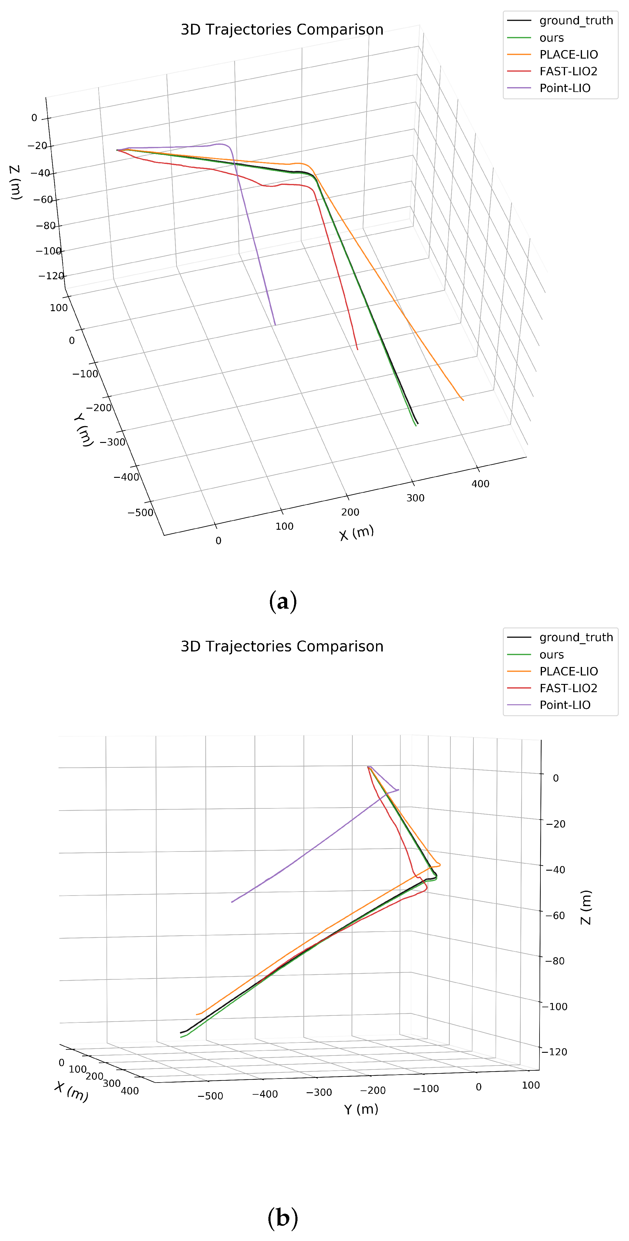
Field tests in a 1.5 km mining tunnel validate the system’s superior performance: compared with existing algorithms, it maintains sub-meter localization accuracy and full-area coverage, with significant improvements in positioning stability. Under severe wheel slip, the anti-slip module reduces velocity error by 74.9%, effectively suppressing slippage-induced disturbances; with prior map correction, the system achieves much lower maximum localization error compared to uncorrected conditions, further enhancing long-range navigation reliability. This system fills the gap in high-reliability, self-contained localization for kilometer-scale underground mining vehicles, meeting the precision and safety demands of autonomous mining operations.

