Machine Learning Methods for Inferring the Number of UAV Emitters via Massive MIMO Receive Array

Abstract

To provide important prior knowledge for the direction of arrival (DOA) estimation of UAV emitters in future wireless networks, we present a complete DOA preprocessing system for inferring the number of emitters via a massive multiple-input multiple-output (MIMO) receive array. Firstly, in order to eliminate the noise signals, two high-precision signal detectors, the square root of the maximum eigenvalue times the minimum eigenvalue (SR-MME) and the geometric mean (GM), are proposed. Compared to other detectors, SR-MME and GM can achieve a high detection probability while maintaining extremely low false alarm probability. Secondly, if the existence of emitters is determined by detectors, we need to further confirm their number. Therefore, we perform feature extraction on the the eigenvalue sequence of a sample covariance matrix to construct a feature vector and innovatively propose a multi-layer neural network (ML-NN). Additionally, the support vector machine (SVM) and naive Bayesian classifier (NBC) are also designed. The simulation results show that the machine learning-based methods can achieve good results in signal classification, especially neural networks, which can always maintain the classification accuracy above 70% with the massive MIMO receive array. Finally, we analyze the classical signal classification methods, Akaike (AIC) and minimum description length (MDL). It is concluded that the two methods are not suitable for scenarios with massive MIMO arrays, and they also have much worse performance than machine learning-based classifiers.

1. Introduction

With the advantages of high mobility and low cost, unmanned aerial vehicles (UAVs) play important roles in wireless networks for implementing tasks like weather monitoring, traffic control, emergency search, communication relaying, etc. [1]. However, unlike traditional ground-to-ground (G2G) communications, UAV communications have some special characteristics and challenges, e.g., the high mobility leads to the UAV communication channels changing much faster, the high flight altitude requires the ground base stations to provide larger 3D signal coverage for UAVs, and the line of sight (LoS) paths between UAVs and base stations are vulnerable to interference from ground users over the same frequency [2]. As is known to us, massive multiple-input multiple-output (MIMO) is a key technology in 5G or future 6G systems [3,4]; it can make significant improvements in system capacity, reliability, and spectral efficiency by using techniques such as spatial multiplexing, diversity, and beamforming [5]. Compared to small arrays, the higher array gain of massive MIMO arrays can make a great extension of signal coverage [6], and experimental results in [7] showed massive MIMO works well with LoS mobile channels. So in view of the problems that UAV communications face, it is natural to consider the combination of UAVs and massive MIMO technology [8]. In [9], a nonstationary 3D geometry-based model was proposed for UAV-to-ground massive MIMO channels; this model considered the realistic scenarios and discussed the impact of some important UAV parameters such as altitude and flight velocity, so it can give some inspiration for future research on 6G standard UAV channel models. As UAVs often appear as clusters, the potential of massive MIMO ground station communication with UAV swarms was explored in [10], and a realistic geometric model was also developed.

Because of the high mobility of UAVs, it is necessary for ground base stations to obtain direction-of-arrival (DOA) information of UAVs in a timely manner for channel estimation and communication security. For most DOA estimation algorithms, such as MUSIC and ESPRIT, the number of emitters is required prior knowledge, but the number is usually unknown [11]. So inferring the number of emitters has been an active topic in array processing for a few decades [12]. In recent years, the potential of massive MIMO technology in array processing has also been gradually discovered [13], as the larger number of antennas can decrease the beamwidth and then increase the angular resolution of the arrays [14]. Therefore, considering the realistic needs of UAV communications and the advantages of massive MIMO technology in array processing, we will study the methods for inferring the number of UAV emitters via a massive MIMO receive array in this work.

In general, the solutions for inferring the number of emitters can be divided into two main categories. The first is based on the information-theoretic criteria and another is based on the analysis of the covariance matrices. Since detecting the number of signal sources can be viewed as a typical model order selection problem, Akaike firstly proposed a method focusing on finding the minimum Kullback–Leibler (KL) discrepancy between the probability density function (PDF) of obtained data and that of models for selection [15], and this method is now called AIC. Schwarz introduced Bayesian information criterion (BIC) based on Akaike’s work [16], and Rissanen also derived a similar criterion called MDL [17]. Ref. [18] provided a good summary of these classical information criteria. In the last decade, Lu and Zoubir proposed the generalized Bayesian information criterion (GBIC) [19] and flexible detection criterion (FDC) [20], which effectively improved the performance on source enumeration. The other basic method for enumerating the number of sources is performing analysis on the covariance matrices of signals received by arrays. Williams and Johnson proposed a sphericity test for source enumeration in [21], which was based on a hypothesis test for the covariance matrix. Ref. [22] gave a bootstrap-based method to estimate the null distributions of the test statistics. Wax and Adler solved this problem by performing signal subspace matching [23].

Signal detection is another technique adopted in this work. In order to reduce the interference of the noise to the detection of signal number, some good methods were proposed, such as classic signal detection algorithms containing energy detection [24], matched-filter detection [25], cyclostationarity-based detection [26], etc. On the basis of these methods, Zeng and Liang proposed two eigenvalue-based algorithms in [27], Zhang et al. used the generalized likelihood ratio test (GLRT) approach to improve detection performance [28], and an eigenvalue-based LRT algorithm was also given in [29].

In recent years, machine learning (ML) has played an important role in the fields of array signal processing [30] and UAV communications [31], and now the ML-based methods used in 5G mainly include supervised learning, unsupervised learning, and reinforcement learning [32]. Thilina et al. compared the performance of unsupervised learning approaches and supervised learning approaches for cooperative spectrum sensing [33]. A machine learning-based DOA measurement method was also proposed in [34], and ref. [35] used a neural network for power allocation in a wireless communication network.

In this paper, we will combine the techniques mentioned above for inferring the number of UAV emitters via massive MIMO receive array. First, the pure noise signals are separated by threshold detectors, and then the feature vectors are extracted from the sample covariance matrices of the remaining signals. Finally, the ML-NN and other machine learning methods are used to classify the signals for determining the number of emitters. Therefore, our main contributions are summarized as follows:

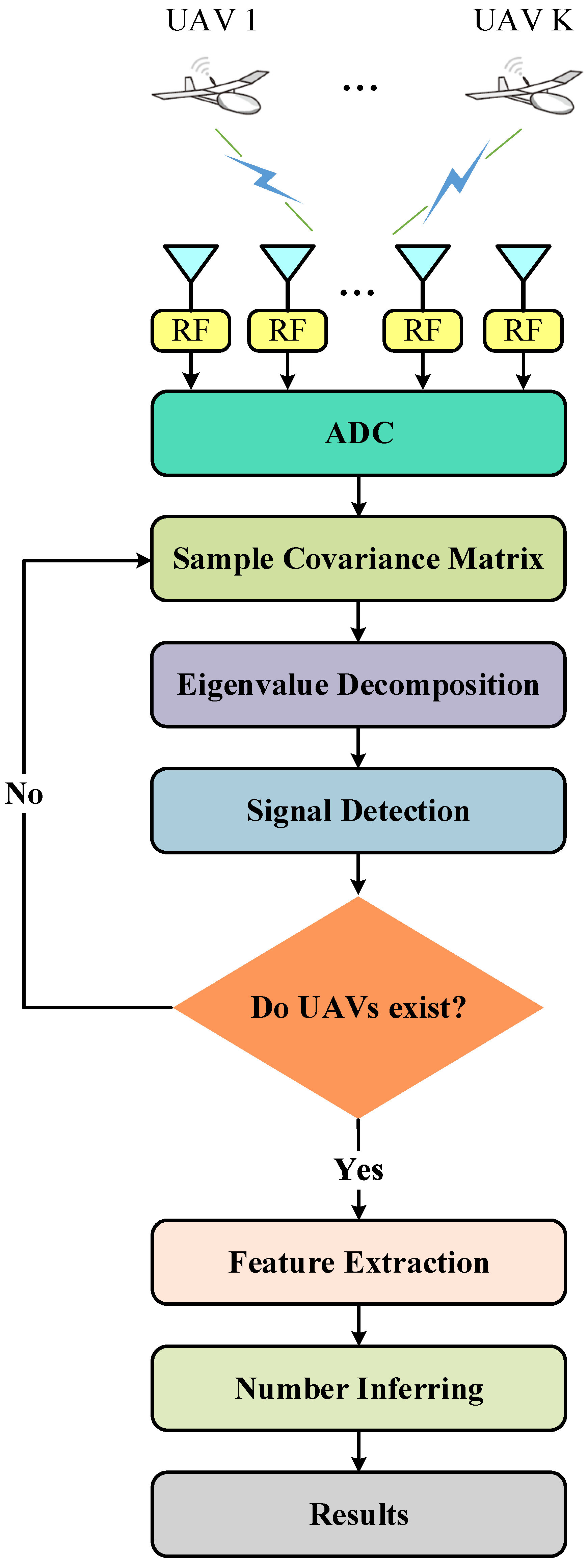
• A DOA preprocessing system is proposed for obtaining the number of UAV emitters via a massive MIMO array. The main steps of this system include signal detection and inferring the number of emitters. The received signals are first inputted into signal detectors. If the detection result shows the presence of emitters, this signal is further transmitted to signal classifiers to determine the number of emitters.
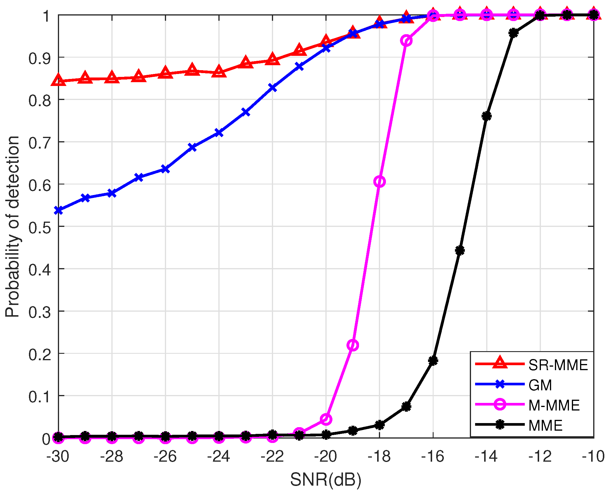
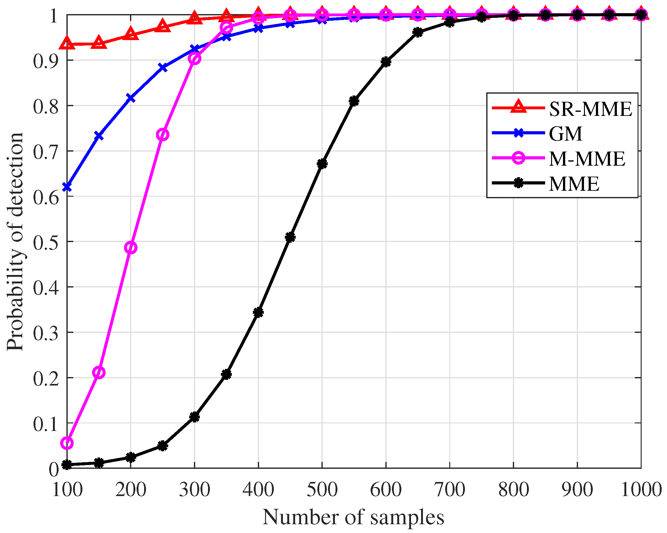
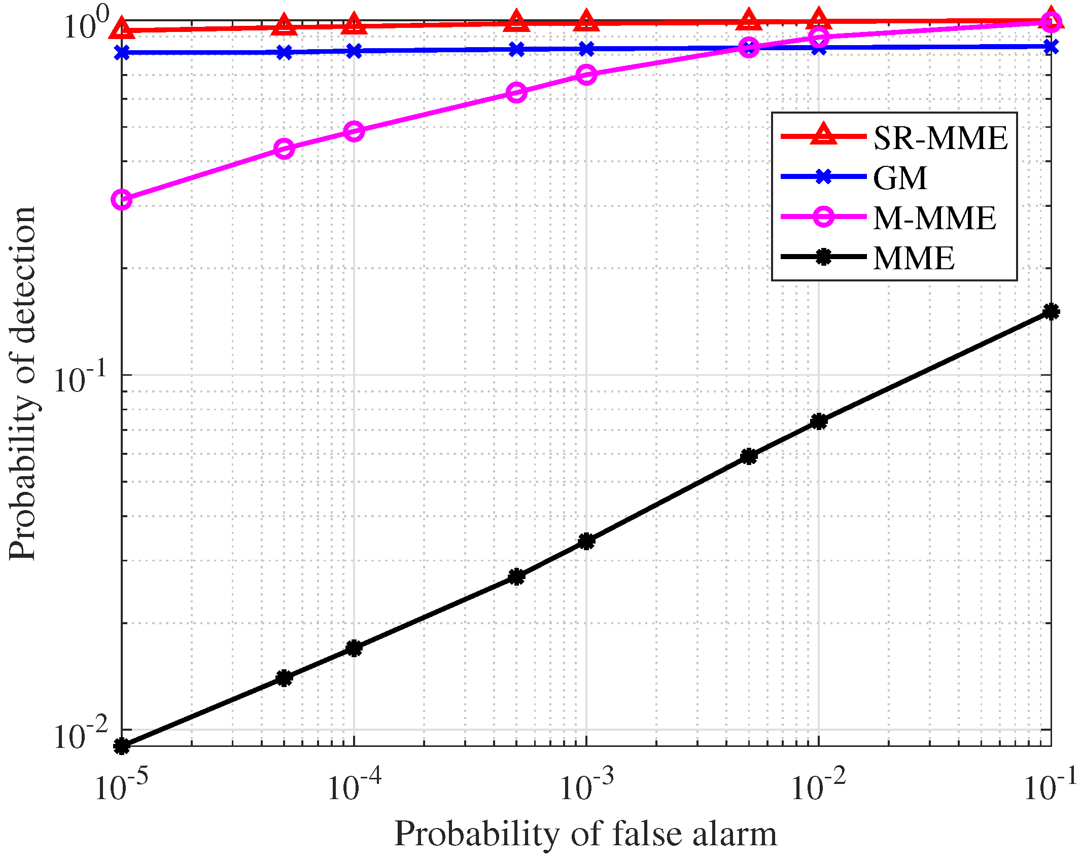
• Two high-precision signal detectors, the square root of the maximum eigenvalue times the minimum eigenvalue (SR-MME) and the geometric mean (GM), are proposed in Section 3. Their thresholds and probability of detection are also derived with the aid of random matrix theories. The simulation results show that SR-MME and GM have significant improvement in detection performance compared with the MME detector proposed in [27] and the M-MME detector proposed in [36], even though the SNR is very low and the number of samples is small. The simulation results also show that SR-MME and GM can maintain a low false alarm probability while achieving a high detection probability.
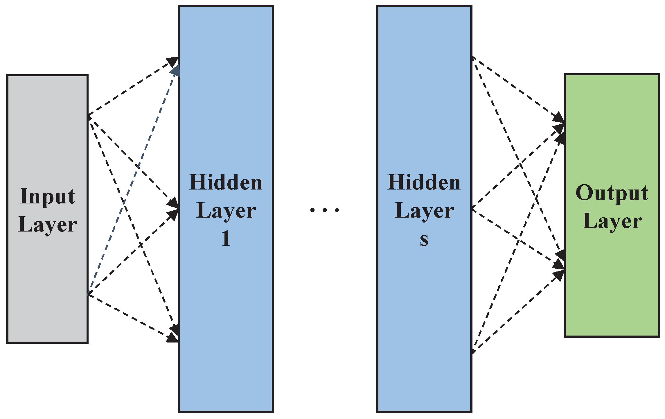
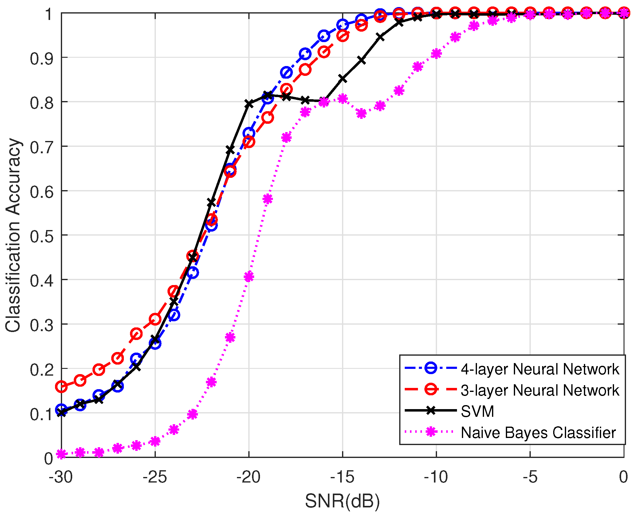
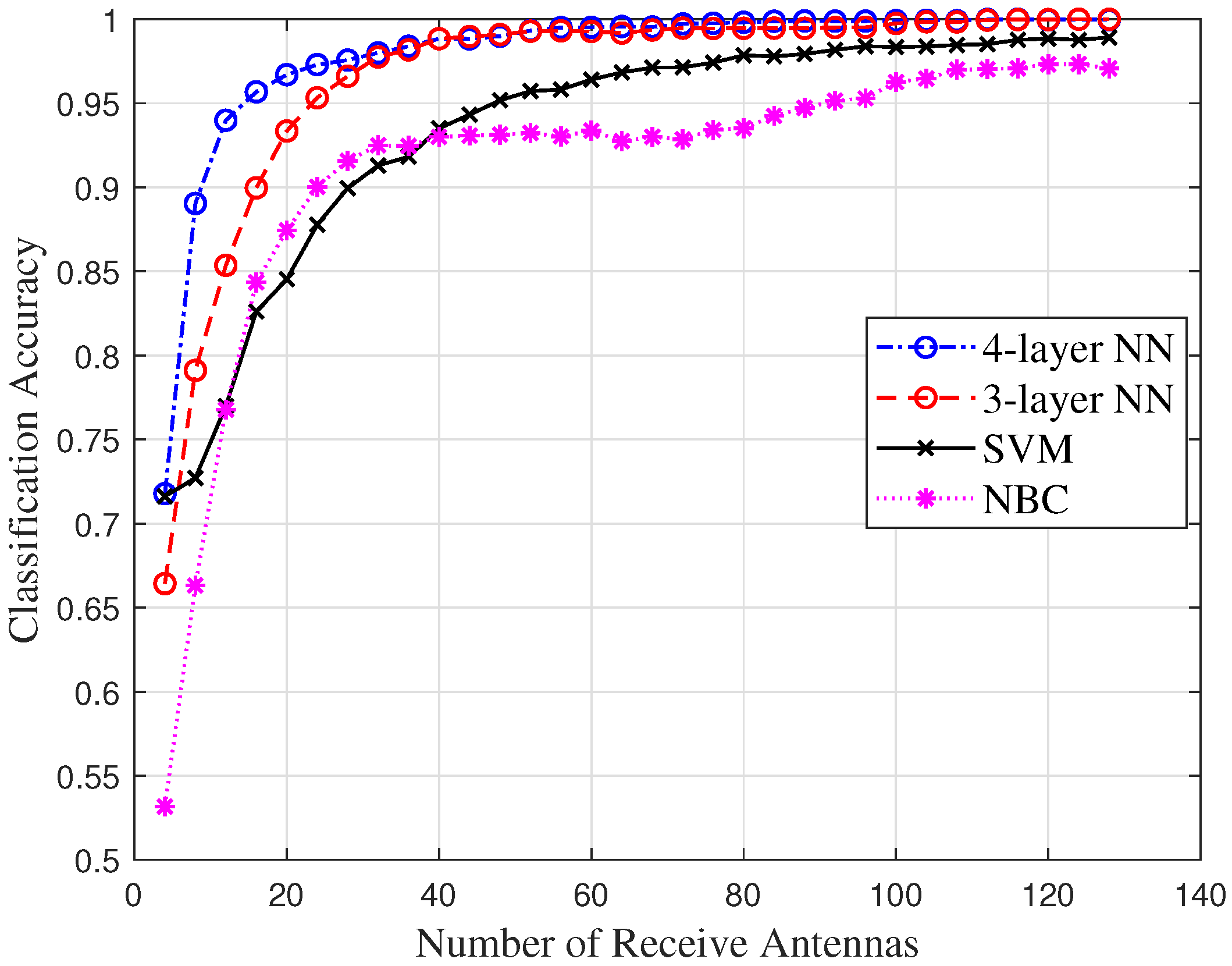
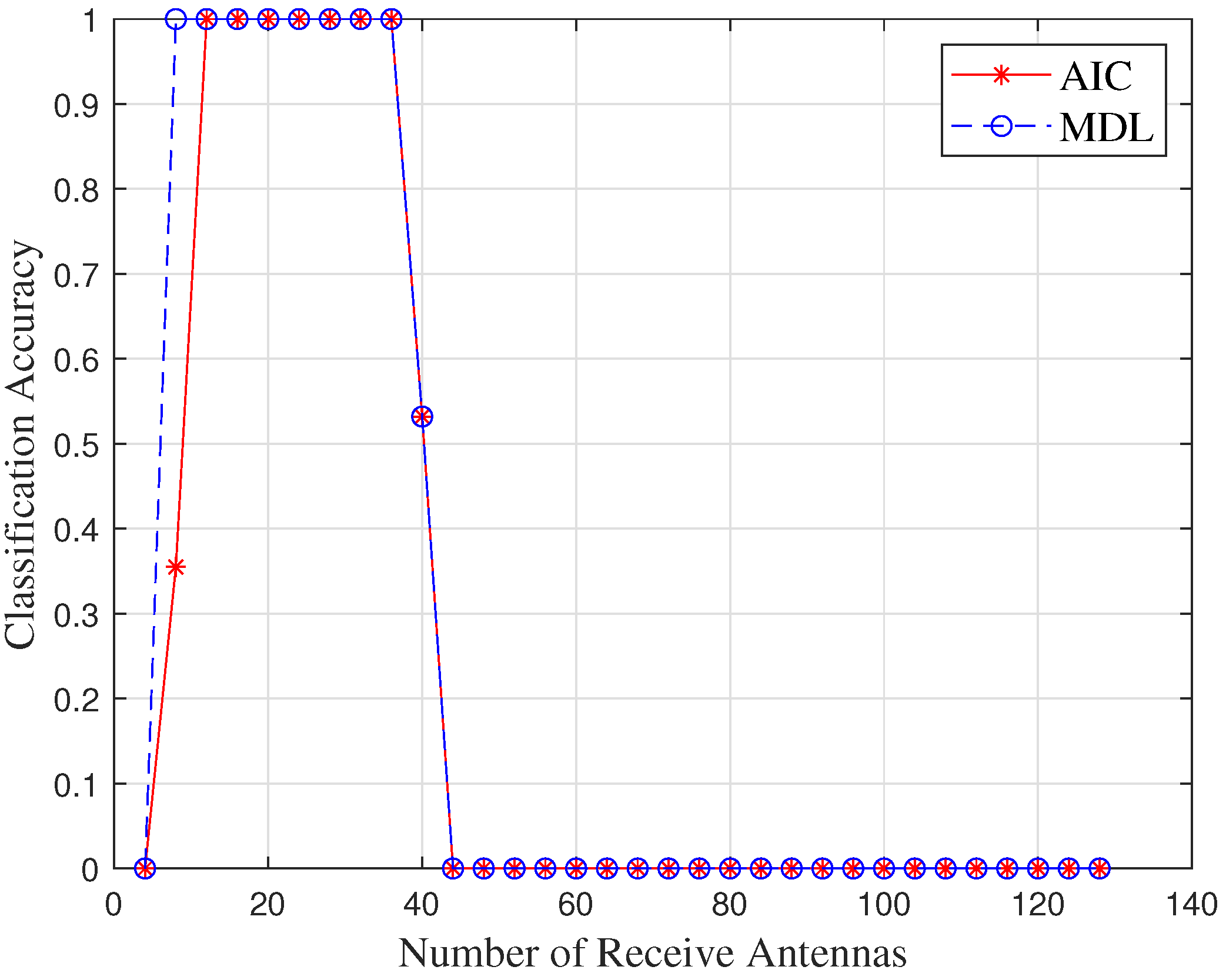
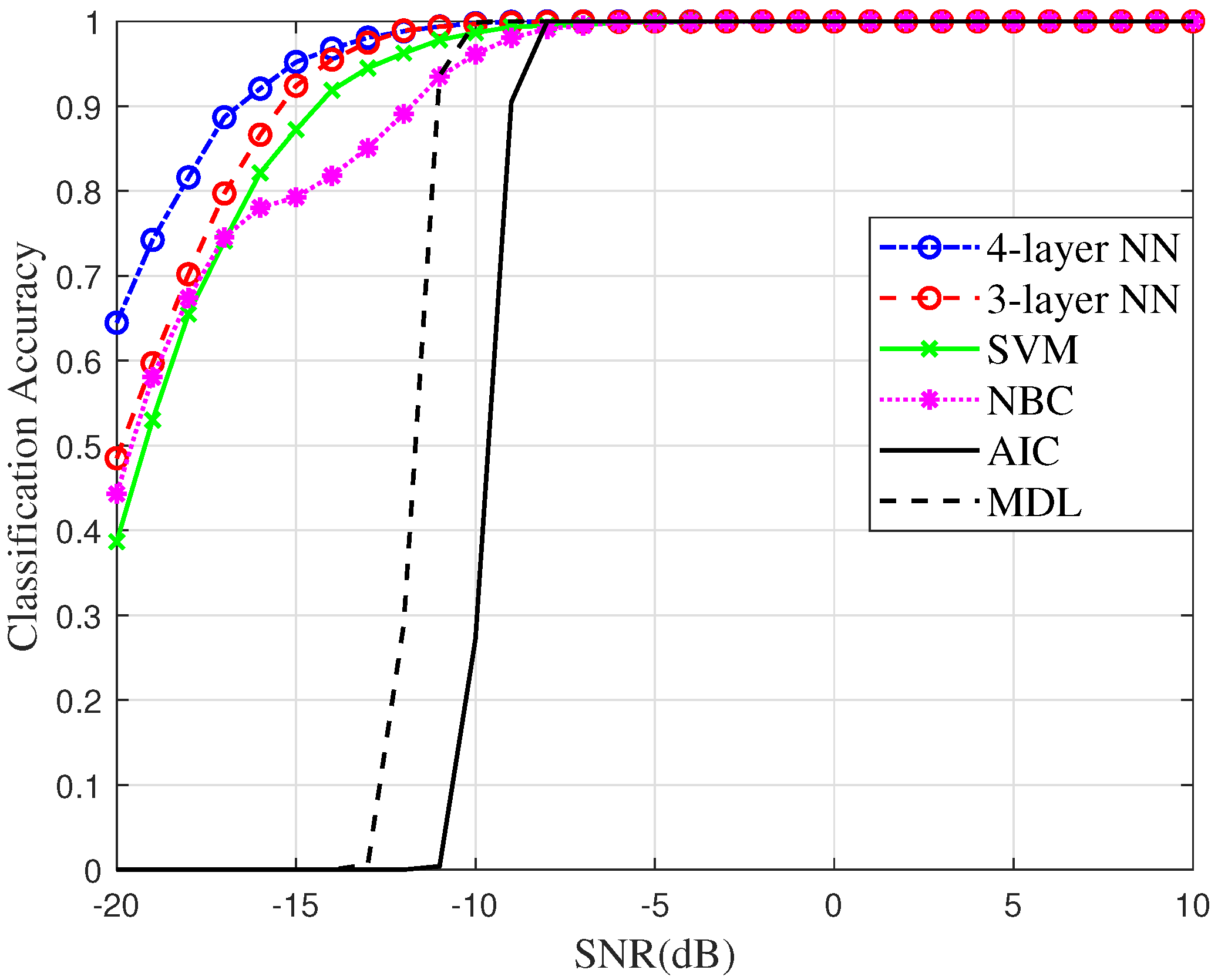
• Since the existence of emitters is known, we innovatively introduce machine learning-based classifiers to infer their number, including multi-layer neural networks (ML-NNs), support vector machine (SVM), and naive Bayesian classifier (NBC). Important features which make up feature vectors are also extracted from eigenvalue sequences of signals’ sample covariance matrices. The results show that machine learning methods are very suitable for performing signal classification, especially neural networks, because they can achieve a classification accuracy of 70%, even under extreme conditions. Finally, we validate the classification performance of AIC and MDL under different SNR and number of receive antennas. We show that they are unapplicable to scenarios with low SNR and massive MIMO receive arrays compared to machine learning-based methods.

The rest of the paper is organized as follows. In Section 2, we present a specific system model and assumptions. Two high-precision signal detectors are given in Section 3. Section 4 shows how to perform feature extraction on received signals and classify them by machine learning methods. Then, the advantages of the proposed detectors and classifiers are presented through simulation results in Section 5. Finally, Section 6 draws conclusions.

Notation: Matrices, vectors, and scalars are denoted by letters of bold upper case, bold lower case, and lower case, respectively. Signs ${(·)}^T$, ${(·)}^{\ast }$, and ${(·)}^H$ represent transpose, conjugate, and conjugate transpose. ${\mathbf{I}}_M$ denotes the $M\times M$ identity matrix. $\mathrm{diag}\{·\}$ stands for diagonal matrix.

2. System Model

As the system shown in Figure 1, we consider a scenario with K far-field UAV emitters and one massive MIMO receiver equipped with an M-element uniform linear array (ULA). The signals transmitted by the kth UAV are denoted by $s_k\left(t\right)e^{j2\pi f_{c}t}$, where $s_k\left(t\right)$ is the baseband signal and $f_c$ is the carrier frequency. Referring to [37], the received signals at the mth antenna are given by

$$y_m\left(t\right)=\sum _{k=1}^K{s}_k\left(t\right)e^{j2\pi f_{c}t}{e}^{-j2\pi f_c{\tau }_{k,m}}+v_m\left(t\right),$$

(1)

where $v_m\left(t\right)\sim \mathcal{CN}(0,{\sigma }_v^2)$ represents the additive white Gaussian noise (AWGN) term, and ${\tau }_{k,m}$ denotes the propagation delay from the kth UAV to the mth antenna, expressed by

$${\tau }_{k,m}={\tau }_0-\frac{(m-1)dsin{\theta }_k}{c},$$

(2)

where ${\tau }_0$ is the propagation delay from the UAV to the reference point on the receive array, ${\theta }_k$ is the angle of signal incidence from the kth UAV, $d=\lambda /2$ represents the space between array elements, and c denotes the speed of light. Then received signals go through ADC and down converter, and we obtain

$$y_m\left(n\right)=\sum _{k=1}^K{e}^{-j2\pi (m-1)d sin {\theta }_k/\lambda }{s}_k\left(n\right)+v_m\left(n\right),$$

(3)

and by combining all the M antennas, we obtain

$$\mathbf{y}\left(n\right)=\sum _{k=1}^K\mathbf{a}\left({\theta }_k\right)s_k\left(n\right)+\mathbf{v}\left(n\right),$$

(4)

where $\mathbf{v}\left(n\right)={[v_1\left(n\right),\dots ,v_M\left(n\right)]}^T$ denotes the noise vector and

$$\mathbf{a}\left({\theta }_k\right)={[1,e^{-j2\pi d sin {\theta }_k/\lambda },\dots ,e^{-j2\pi (M-1)d sin {\theta }_k/\lambda }]}^T,$$

(5)

is the array manifold.

Initially, it is not clear whether the UAVs exist, so we should consider two situations, including the signals’ presence and only noise [38]. By turning (4) to matrix form, we obtain

$$H_0:\mathbf{y}\left(n\right)=\mathbf{v}\left(n\right)H_1:\mathbf{y}\left(n\right)=\mathbf{A}\mathbf{s}\left(n\right)+\mathbf{v}\left(n\right),$$

(6)

where $\mathbf{s}\left(n\right)={[s_1\left(n\right),\dots ,s_K\left(n\right)]}^T$, $\mathbf{A}=[\mathbf{a}\left({\theta }_1\right),\dots ,\mathbf{a}\left({\theta }_K\right)]$. Then the covariance matrix of the received signal can be expressed by

$${\mathbf{Q}}_{\mathbf{y}}=\mathbf{A}{\mathbf{Q}}_{\mathbf{s}}{\mathbf{A}}^H+{\sigma }_{\mathbf{v}}^2{\mathbf{I}}_M=\sum _{k=1}^K{\sigma }_{\mathbf{s},k}^2\mathbf{a}\left({\theta }_k\right){\mathbf{a}}^H\left({\theta }_k\right)+{\sigma }_{\mathbf{v}}^2{\mathbf{I}}_M.$$

(7)

where ${\mathbf{Q}}_{\mathbf{s}}=\mathrm{E}\left[\mathbf{S}\left(\mathrm{n}\right){\mathbf{S}}^{\mathrm{H}}\left(\mathrm{n}\right)\right]$$=\mathrm{diag}\{{\sigma }_{\mathbf{s},1}^2,\dots ,{\sigma }_{\mathbf{s},K}^2\}$.

Since the base station is equipped with a massive array, $M\gg K$ and $\mathrm{rank}\left(\mathrm{A}\right)=K$. Then the eigenvalues of ${\mathbf{Q}}_{\mathbf{y}}$ satisfy the following properties

$$\underset{\mathrm{signal}\mathrm{subspace}}{\underbrace{{\lambda }_1\ge {\lambda }_2\ge \dots \ge {\lambda }_K}}>\underset{\mathrm{noise}\mathrm{subspace}}{\underbrace{{\lambda }_{K+1}=\dots ={\lambda }_M={\sigma }_{\mathbf{v}}^2}},$$

(8)

and

$${\lambda }_m={\rho }_m+{\sigma }_{\mathbf{v}}^2,$$

(9)

where ${\rho }_1\ge \dots \ge {\rho }_K>{\rho }_{K+1}=\dots ={\rho }_M=0$ are the eigenvalues of $\mathbf{A}{\mathbf{Q}}_{\mathbf{s}}{\mathbf{A}}^H$.

In practice, the covariance matrix of received signal $\mathbf{y}$ cannot be obtained accurately, so the sample covariance matrix of the received signal is usually used to approximate it:

$${\widehat{\mathbf{Q}}}_{\mathbf{y}}=\frac{1}{N}\sum _{n=1}^N\mathbf{y}\left(n\right){\mathbf{y}}^H\left(n\right)=\frac{1}{N}\mathbf{Y}{\mathbf{Y}}^H,$$

(10)

where

$$H_0:\mathbf{Y}=\mathbf{V}{H}_1:\mathbf{Y}=\mathbf{A}\mathbf{S}+\mathbf{V},$$

(11)

and $\mathbf{S}=\left[\mathbf{s}\right(1),\mathbf{s}(2),\dots ,\mathbf{s}(N\left)\right]$, $\mathbf{V}=\left[\mathbf{v}\right(1),\mathbf{v}(2),\dots ,\mathbf{v}(N\left)\right]$.

Figure 1. The procedure of proposed system for inferring the number of UAV emitters by massive MIMO receive array.

3. Signal Detectors

As shown in Figure 1, after the sample covariance matrix of the received signal is obtained, we take eigenvalue decomposition (EVD) on it. For the two situations in (11), eigenvalues are represented by ${\lambda }_1\left({\widehat{\mathbf{Q}}}_{\mathbf{y},H_0}\right)\ge \dots \ge {\lambda }_M\left({\widehat{\mathbf{Q}}}_{\mathbf{y},H_0}\right)$ and ${\lambda }_1\left({\widehat{\mathbf{Q}}}_{\mathbf{y},H_1}\right)\ge \dots \ge {\lambda }_M\left({\widehat{\mathbf{Q}}}_{\mathbf{y},H_1}\right)$, respectively. For convenience, we consider moving the constant $1/N$ to the left-hand side of (10). Assuming ${\sigma }_{\mathbf{v}}^2=1$, we obtain

$$\begin{array}{cc}\hfill & {\mathbf{R}}_{H_0}=\mathbf{V}{\mathbf{V}}^H,\hfill \end{array}$$

(12a)

$$\begin{array}{cc}\hfill & {\mathbf{R}}_{H_1}=N\mathbf{A}{\widehat{\mathbf{Q}}}_{\mathbf{S}}{\mathbf{A}}^H+{\mathbf{R}}_{H_0},\hfill \end{array}$$

(12b)

where ${\mathbf{R}}_{H_0}$ is a Wishart matrix and ${\widehat{\mathbf{Q}}}_{\mathbf{S}}$ is the sample covariance matrix of $\mathbf{S}$. The eigenvalues of ${\mathbf{R}}_{H_0}$ and ${\mathbf{R}}_{H_1}$ can also be expressed as ${\lambda }_1\left({\mathbf{R}}_{H_0}\right)\ge \dots \ge {\lambda }_M\left({\mathbf{R}}_{H_0}\right)$ and ${\lambda }_1\left({\mathbf{R}}_{H_1}\right)\ge \dots \ge {\lambda }_M\left({\mathbf{R}}_{H_1}\right)$, where ${\lambda }_m\left({\mathbf{R}}_{H_0}\right)=N{\lambda }_m\left({\widehat{\mathbf{Q}}}_{\mathbf{y},H_0}\right)$ and ${\lambda }_m\left({\mathbf{R}}_{H_1}\right)=N{\lambda }_m\left({\widehat{\mathbf{Q}}}_{\mathbf{y},H_1}\right)$. Since ${\mathbf{R}}_{H_0}$ is a complex Gaussian Wishart matrix, its largest eigenvalue should follow Tracy–Widom distribution of order 2 [39]:

$$\frac{{\lambda }_{\max }\left({\mathbf{R}}_{H_0}\right)-\mu }{\nu }\stackrel{d}{\to }{\mathcal{TW}}_2,$$

(13)

where

$$\begin{array}{cc}\hfill & \mu ={(\sqrt{M}+\sqrt{N})}^2,\hfill \end{array}$$

(14a)

$$\begin{array}{cc}\hfill & \nu =\sqrt{\mu }{\left(\frac{1}{\sqrt{M}}+\frac{1}{\sqrt{N}}\right)}^{1/3},\hfill \end{array}$$

(14b)

are center and scaling parameters. Then the cumulative distribution function (CDF) of the largest eigenvalue, i.e., $F\left(x\right)$, can be approximated as

$$F\left(x\right)\approx F_2\left(\frac{x-\mu }{\nu }\right),$$

(15)

where $F_2\left(x\right)$ denotes the distribution function of ${\mathcal{TW}}_2$. Referring to [40,41], it is defined as

$$F_2\left(x\right)=\exp \left\{-{\int }_x^{\infty }(a-x)q^2\left(a\right)da\right\},$$

(16)

where $q\left(a\right)$ is the solution of Painlevé II differential equation

$$q^{″}\left(a\right)=aq\left(a\right)+2q^3\left(a\right).$$

(17)

with boundary condition $q\left(a\right)\sim Ai\left(a\right)$ as $a\to \infty$, where $Ai\left(a\right)$ represents the Airy function [42]. The value of $F_2\left(x\right)$ can be computed by using software packages such as [43].

In addition, for the Wishart matrix ${\mathbf{R}}_{H_0}$, if $\underset{N\to +\infty }{lim}\frac{M}{N}=z(z\in [0,1])$, its maximum and minimum eigenvalues can be approximated as ${(\sqrt{N}+\sqrt{M})}^2$ and ${(\sqrt{N}-\sqrt{M})}^2$, respectively. Next we will present several high-performance signal detectors based on the knowledge given earlier.

3.1. Proposed SR-MME Detector

The SR-MME detector is defined as the square root of the maximum eigenvalue times the minimum eigenvalue, and is given by

$$\sqrt{{\lambda }_{\max }\left({\widehat{\mathbf{Q}}}_{\mathbf{y}}\right){\lambda }_{\min }\left({\widehat{\mathbf{Q}}}_{\mathbf{y}}\right)}\underset{H_0}{\overset{H_1}{\gtrless }}{\gamma }_1,$$

(18)

where ${\lambda }_{\max }\left({\widehat{\mathbf{Q}}}_{\mathbf{y}}\right)$, ${\lambda }_{\min }\left({\widehat{\mathbf{Q}}}_{\mathbf{y}}\right)$ are maximum and minimum eigenvalues, respectively, of sample covariance matrix ${\widehat{\mathbf{Q}}}_{\mathbf{y}}$, and ${\gamma }_1$ denotes the judgment threshold.

At the end of judgment, there will be four possible results: true positive (TP), false positive (FP), true negative (TN), false negative (FN). From a probabilistic perspective, we know $P_{TP}+P_{TN}=1$ and $P_{FP}+P_{FN}=1$, where the probability of FP is also called false alarm (FA) probability, so only TP and FP situations need to be addressed. Therefore, $P_{FA}$ of the SR-MME detector is defined as

$$\begin{array}{cc}\hfill P_{FA}& =P\left(\sqrt{{\lambda }_{\max }\left({\widehat{\mathbf{Q}}}_{\mathbf{y},H_0}\right){\lambda }_{\min }\left({\widehat{\mathbf{Q}}}_{\mathbf{y},H_0}\right)}>{\gamma }_1\right)\hfill \\ \hfill & =P\left({\lambda }_{\max }\left({\mathbf{R}}_{H_0}\right)>\frac{{\left(N{\gamma }_1\right)}^2}{{\lambda }_{\min }\left({\mathbf{R}}_{H_0}\right)}\right)\hfill \\ \hfill & =P\left(\frac{{\lambda }_{\max }\left({\mathbf{R}}_{H_0}\right)-\mu }{\nu }>\frac{{\left(\frac{N{\gamma }_1}{\sqrt{N}-\sqrt{M}}\right)}^2-\mu }{\nu }\right)\hfill \\ \hfill & =1-F_2\left(\frac{{\left(\frac{N{\gamma }_1}{\sqrt{N}-\sqrt{M}}\right)}^2-\mu }{\nu }\right).\hfill \end{array}$$

(19)

Then the threshold can be derived as

$${\gamma }_1=\frac{\sqrt{N}-\sqrt{M}}{N}\sqrt{\nu F_2^{-1}(1-P_{FA})+\mu }.$$

(20)

When the signal exists, the sample covariance matrix (12a) is no longer a Wishart matrix. As shown in [27], its maximum and minimum eigenvalues can be approximated as

$$\begin{array}{cc}\hfill {\lambda }_{\max }\left({\mathbf{R}}_{H_1}\right)& \approx N{\rho }_1+{\lambda }_{\max }\left({\mathbf{R}}_{H_0}\right),\hfill \end{array}$$

(21a)

$$\begin{array}{cc}\hfill {\lambda }_{\min }\left({\mathbf{R}}_{H_1}\right)& \approx N{\rho }_M+\sqrt{N}(\sqrt{N}-\sqrt{M}),\hfill \end{array}$$

(21b)

The detection probability $P_D$, i.e., $P_{TP}$, is given by

$$\begin{array}{cc}\hfill & P_D=P\left(\sqrt{{\lambda }_{\max }\left({\widehat{\mathbf{Q}}}_{\mathbf{y},H_1}\right){\lambda }_{\min }\left({\widehat{\mathbf{Q}}}_{\mathbf{y},H_1}\right)}>{\gamma }_1\right)\hfill \\ \hfill & =P\left({\lambda }_{\max }\left({\mathbf{R}}_{H_1}\right)>\frac{{\left(N{\gamma }_1\right)}^2}{{\lambda }_{\min }\left({\mathbf{R}}_{H_1}\right)}\right)\hfill \\ \hfill & =P\left(\frac{{\lambda }_{\max }\left({\mathbf{R}}_{H_0}\right)-\mu }{\nu }>\frac{\frac{{\left(N{\gamma }_1\right)}^2}{N{\rho }_M+N-\sqrt{MN}}-N{\rho }_1-\mu }{\nu }\right)\hfill \\ \hfill & =1-F_2\left(\frac{\frac{{\left(N{\gamma }_1\right)}^2}{N{\rho }_M+N-\sqrt{MN}}-{\rho }_1-\mu }{\nu }\right).\hfill \end{array}$$

(22)

3.2. Proposed GM Detector

The geometric mean (GM) detector is defined as

$$\sqrt[M]{\prod _{m=1}^M{\lambda }_m\left({\widehat{\mathbf{Q}}}_{\mathbf{y}}\right)}\underset{H_0}{\overset{H_1}{\gtrless }}{\gamma }_2,$$

(23)

where ${\lambda }_m\left({\widehat{\mathbf{Q}}}_{\mathbf{y}}\right)$ is the eigenvalue of the sample covariance matrix and ${\gamma }_2$ represents the judgment threshold of this detector. Similar to SR-MME detector, the false alarm probability of the GM detector is given by

$$\begin{array}{cc}\hfill & P_{FA}=P\left(\sqrt[M]{\prod _{m=1}^M{\lambda }_m\left({\widehat{\mathbf{Q}}}_{\mathbf{y},H_0}\right)}>{\gamma }_2\right)\hfill \\ \hfill & =P\left({\lambda }_{\max }\left({\mathbf{R}}_{H_0}\right)>{\gamma }_2^M\frac{{\lambda }_{\max }\left({\mathbf{R}}_{H_0}\right)}{\det \left({\widehat{\mathbf{Q}}}_{\mathbf{y},H_0}\right)}\right)\hfill \\ \hfill & =P\left(\frac{{\lambda }_{\max }\left({\mathbf{R}}_{H_0}\right)-\mu }{\nu }>\frac{{\gamma }_2^M\frac{{(\sqrt{N}+\sqrt{M})}^2}{\det \left({\widehat{\mathbf{Q}}}_{\mathbf{y},H_0}\right)}-\mu }{\nu }\right)\hfill \\ \hfill & =1-F_2\left(\frac{{\gamma }_2^M\frac{{(\sqrt{N}+\sqrt{M})}^2}{\det \left({\widehat{\mathbf{Q}}}_{\mathbf{y},H_0}\right)}-\mu }{\nu }\right),\hfill \end{array}$$

(24)

and the threshold is

$${\gamma }_2=\sqrt[M]{\frac{\left(\nu F_2^{-1}(1-P_{FA})+\mu \right)\det \left({\widehat{\mathbf{Q}}}_{\mathbf{y},H_0}\right)}{{(\sqrt{N}+\sqrt{M})}^2}}.$$

(25)

Finally, the detection probability of the GM detector can be expressed by

$$\begin{array}{cc}\hfill & P_D=P\left(\sqrt[M]{\prod _{m=1}^M{\lambda }_m\left({\widehat{\mathbf{Q}}}_{\mathbf{y},H_1}\right)}>{\gamma }_2\right)\hfill \\ \hfill & =P\left({\lambda }_{\max }\left({\mathbf{R}}_{H_0}\right)>{\gamma }_2^M\frac{{\lambda }_{\max }\left({\mathbf{R}}_{H_0}\right)}{\det \left({\widehat{\mathbf{Q}}}_{\mathbf{y},H_1}\right)}\right)\hfill \\ \hfill & =1-F_2\left(\frac{{\gamma }_2^M\frac{{(\sqrt{N}+\sqrt{M})}^2}{\det \left({\widehat{\mathbf{Q}}}_{\mathbf{y},H_1}\right)}-\mu }{\nu }\right).\hfill \end{array}$$

(26)

4. Proposed Classifiers for Inferring the Number of UAV Emitters

The detectors proposed in Section 3 are designed for detecting whether the signals received by the base station are from UAV emitters or noise only. If the UAVs are present, we need to further determine their number. Therefore, a multi-layer neural network (ML-NN) classifier is given in the following. Support vector machine (SVM) classifier and naive Bayesian classifier (NBC) are also discussed as benchmarks.

4.1. Feature Selection and Extraction

As can be seen in Figure 1, after the sampling of the received signal, taking eigenvalue decomposition on the sample covariance matrix ${\widehat{\mathbf{Q}}}_{\mathbf{y}}$, we can obtain eigenvalues ${\widehat{\lambda }}_1\ge {\widehat{\lambda }}_2\ge \dots \ge {\widehat{\lambda }}_M$. Although the sample covariance matrix is only an approximation of the actual received signal covariance matrix, its eigenvalues also approximately satisfy (8) if the sample number N is large enough, i.e., the maximum K eigenvalues belong to signal subspace. Therefore, this character can be used to determine the number of signal emitters. Firstly, the following features of ${\left\{{\widehat{\lambda }}_m\right\}}_{m=1}^M$ are selected to construct the feature space of received signal $\mathbf{Y}$, where

$$\left\{\begin{array}{c}{\widehat{\lambda }}_{\max },{\widehat{\lambda }}_{\min }\hfill \\ \overline{\lambda }=\frac{1}{M}\sum _{m=1}^M{\widehat{\lambda }}_m,\tilde{\lambda }={\left(\prod _{m=1}^M{\widehat{\lambda }}_m\right)}^{1/M}\hfill \\ {\sigma }_{\widehat{\lambda }}=\sqrt{\frac{{\sum }_{m=1}^M{({\widehat{\lambda }}_m-\overline{\lambda })}^2}{M}}.\hfill \end{array}\right.$$

(27)

As the number of emitters grows, the features also increase. In order to enlarge the discrimination between the different signals, we perform log operations on them. Then, the feature vector of any received signal is given by

$$\mathbf{x}=\left(log\left({\widehat{\lambda }}_{\max }\right),log\left({\widehat{\lambda }}_{\min }\right),log\left(\overline{\lambda }\right),log\left(\tilde{\lambda }\right),log\left({\sigma }_{\widehat{\lambda }}\right)\right).$$

(28)

Since the signal received by the base station is derived from different emitters, and it is a typical multiclass problem, machine learning-based methods are very suitable. Assuming there are most K emitters in the coverage area of the base station, we can obtain a K-elements classifier based on the existing training data and then substitute the signal to be detected into this classifier for classification. Then we will introduce several high-performance classification algorithms.

4.2. Proposed Multi-Layer Neural Network Classifier

We first take a set of received signals for training, such as $\mathbf{X}={\left\{({\mathbf{x}}_i,{\mathbf{g}}_i)\right\}}_{i=1,2,\dots }$, where ${\mathbf{g}}_i=[g_{i,1},\dots ,g_{i,k},\dots ,g_{i,K}]$ is the corresponding output vector. It is a unit vector if signal i belongs to class k, $g_{i,k}=1$. As is shown in Figure 2, the input of this neural network is a feature vector defined in (28), and the input layer is constructed of five neurons. Since most K emitters are in the coverage area of the base station, the number of neurons in the output layer is also K and the outputs of these neurons are denoted by $\{{\widehat{g}}_1,{\widehat{g}}_2,\dots ,{\widehat{g}}_K\}$. Assuming there are a total s hidden layers in this network, these hidden layers contain $q_1,q_2,\dots ,q_s$ neurons, respectively. Therefore, referring to [44], the input received by the $j_1$th neuron of hidden layer 1 can be represented as

$${\alpha }_{1,j_1}=\sum _{h=1}^5{v}_{h,j_1}\mathbf{x}\left(h\right),$$

(29)

where $v_{h,j_1}$ is the connection coefficient between the hth neuron of the input layer and the $j_1$th neuron of hidden layer 1. Then, the output of this neuron is given by

$$z_{j_1}^1=f({\alpha }_{1,j_1}-{\delta }_{1,j_1}),$$

(30)

where ${\delta }_{1,j_1}$ denotes the threshold of the jth neuron of hidden layer 1. $f(·)$ is the activation function, and usually a sigmoid function is adopted, which can be defined as

$$\mathrm{sigmoid}\left(x\right)=\frac{1}{1+e^{-x}}.$$

(31)

We can deduce the input and output of the rest of the hidden layers from hidden layer 1, and the output from the $j_s$th neuron of hidden layer s is given as

$$\begin{array}{cc}\hfill z_{j_s}^s& =f({\alpha }_{s,j_s}-{\delta }_{s,j_s})\hfill \\ \hfill & =f\left(\sum _{j_{s-1}=1}^{q_{s-1}}{u}_{j_{s-1},j_s}{z}_{j_{s-1}}^{s-1}-{\delta }_{s,j_s}\right),\hfill \end{array}$$

(32)

where $u_{j_{s-1},j_s}$ represents the connection coefficient between the $j_{s-1}$th neuron of hidden layer $s-1$ and the $j_s$th neuron of hidden layer s. Since the output of the last hidden layer is transmitted to the output layer, the final output of this network is

$${\widehat{g}}_k=f({\beta }_k-{\epsilon }_k)=f\left(\sum _{j_s=1}^{q_s}{w}_{j_s,k}{z}_{j_s}^s-{\epsilon }_k\right),$$

(33)

where $w_{j_s,k}$ is the connection coefficient between hidden layer s and the output layer, and ${\epsilon }_k$ is the threshold of the kth neuron of the output layer.

When the input signal is ${\mathbf{x}}_1$, the ideal output is ${\mathbf{g}}_i$. However, the actual output of this neural network is ${\widehat{\mathbf{g}}}_i=[{\widehat{g}}_{i,1},\dots ,{\widehat{g}}_{i,k},\dots ,{\widehat{g}}_{i,K}]$, then the mean squared error (MSE) between ideal output and actual output is derived as

$$E_i=\frac{1}{K}\sum _{k=1}^K{\left({\widehat{g}}_{i,k}-g_{i,k}\right)}^2,$$

(34)

Based on the classification error, we can update all the $(5q_1+{\sum }_{t=1}^{s-1}{q}_t{q}_{t+1}+q_{s}K)$ connection coefficients and $({\sum }_{t=1}^s{q}_t+K)$ thresholds of this neural network. Taking the $j_s$th neuron of hidden layer s as an example, we obtain

$$\begin{array}{cc}\hfill w_{j_s,k}^{l+1}& =w_{j_s,k}^l+\Delta w_{j_s,k}^l,\hfill \end{array}$$

(35a)

$$\begin{array}{cc}\hfill {\delta }_{s,j_s}^{l+1}& ={\delta }_{s,j_s}^l+\Delta {\delta }_{s,j_s}^l,\hfill \end{array}$$

(35b)

where l represents the number of iterations. According to the gradient descent method, the update terms are defined as

$$\begin{array}{cc}\hfill \Delta w_{j_s,k}^l& =-\eta \frac{\partial E_i}{\partial w_{j_s,k}^l}\hfill \\ \hfill & =-\eta \frac{\partial E_i}{\partial {\widehat{g}}_{i,k}}·\frac{\partial {\widehat{g}}_{i,k}}{\partial {\beta }_k}·\frac{\partial {\beta }_k}{\partial w_{j_s,k}^l}\hfill \\ \hfill & =-\frac{2\eta }{K}{z}_{j_s}^s·G_{i,k},\hfill \end{array}$$

(36)

and

$$\begin{array}{cc}\hfill \Delta {\delta }_{s,j_s}^l& =-\eta \frac{\partial E_i}{\partial {\delta }_{s,j_s}^l}\hfill \\ \hfill & =-\eta \sum _{k=1}^K\frac{\partial E_i}{\partial {\widehat{g}}_{i,k}}·\frac{\partial {\widehat{g}}_{i,k}}{\partial {\beta }_k}·\frac{\partial {\beta }_k}{\partial z_{j_s}^s}·\frac{\partial z_{j_s}^s}{\partial {\delta }_{s,j_s}^l}\hfill \\ \hfill & =-\frac{2\eta }{K}{z}_{j_s}^s(1-z_{j_s}^s)·\sum _{k=1}^K{w}_{j_s,k}^l{G}_{i,k},\hfill \end{array}$$

(37)

where $\eta$ is the learning rate and

$$G_{i,k}={\widehat{g}}_{i,k}(1-{\widehat{g}}_{i,k})({\widehat{g}}_{i,k}-g_{i,k}).$$

(38)

All the parameters in the neural network are updated in each iteration until the parameters change less than a certain threshold or a certain number of iterations is reached. Therefore, the final classification result for signal i is given by

$$C_i=arg\underset{k}{max}{\widehat{g}}_{i,k}^L,$$

(39)

where $C_i\in \{1,2,\dots ,K\}$.

Figure 2. Multi-layer neural network.

4.3. Support Vector Machine Classifier

Since determining the number of signal sources is a K-elements classification problem, it can be decomposed into $K(K-1)/2$ binary classification problems and each of these binary classification problems can be solved by the support vector machine (SVM) method. Given a training sample set $D=\{({\mathbf{x}}_1,g_1),({\mathbf{x}}_2,g_2),\dots ,({\mathbf{x}}_s,g_s)\}$, where $g_i=\{-1,+1\}$, $g_i=-1$ denotes that signal i belongs to class 1 and $g_i=+1$ denotes that this signal belongs to class 2. The separable hyperplane for the sample space can be expressed by

$${\mathbf{w}}^T\mathbf{x}+b=0,$$

(40)

where $\mathbf{w}$ is the normal vector which determines the direction of this hyperplane, and b denotes the bias which is defined as the distance from the hyperplane to the original point. Therefore, the separable hyperplane can be denoted as $(\mathbf{w},b)$.

Assuming the samples can be classified by hyperplane $(\mathbf{w},b)$ accurately, if $g_i=-1$, we can obtain ${\mathbf{w}}^T{\mathbf{x}}_i+b<0$, and if $g_i=+1$, we obtain ${\mathbf{w}}^T{\mathbf{x}}_i+b>0$. Then the following conditions should be satisfied:

$$\left\{\begin{array}{c}{\mathbf{w}}^T{\mathbf{x}}_i+b\ge +1,g_i=+1\hfill \\ {\mathbf{w}}^T{\mathbf{x}}_i+b\le -1,g_i=-1.\hfill \end{array}\right.$$

(41)

The samples closest to the separable hyperplane make the equalities in (41) hold, and they are support vectors. The sum of the distance from the two heterologous support vectors to the hyperplane is called the margin, and it is defined as $\delta =\frac{2}{\parallel \mathbf{w}\parallel }$. For maximizing the margin of the separable hyperplane, the optimization problem can be designed as

$$\begin{array}{cc}\hfill \underset{\mathbf{w},b}{min}& \frac{1}{2}{\parallel \mathbf{w}\parallel }^2\hfill \end{array}$$

(42a)

$$\begin{array}{cc}\hfill \mathrm{s}.\mathrm{t}.& g_i({\mathbf{w}}^T{\mathbf{x}}_i+b)\ge 1.\hfill \end{array}$$

(42b)

Actually, the training samples can hardly be linearly separated in the current sample space. Firstly, we map the samples to a higher-dimensional feature space. Then the model of the separable hyperplane is modified as

$$f\left(\mathbf{x}\right)={\mathbf{w}}^T\varphi \left(\mathbf{x}\right)+b.$$

(43)

Secondly, to avoid overfitting, we introduce the concept of soft margin. This concept allows SVM to make errors in the classification of some samples, i.e., these samples can not satisfy constraint $g_i({\mathbf{w}}^T\varphi \left({\mathbf{x}}_i\right)+b)\ge 1$. Consequently, the optimization problem (42) is transformed to maximize the margin while minimizing the classification error:

$$\begin{array}{cc}\hfill \underset{\mathbf{w},b,{\xi }_i}{min}& \frac{1}{2}{\parallel \mathbf{w}\parallel }^2+C\sum _{i=1}^s{\xi }_i,\hfill \end{array}$$

(44a)

$$\begin{array}{cc}\hfill \mathrm{s}.\mathrm{t}.& g_i({\mathbf{w}}^T\varphi \left({\mathbf{x}}_i\right)+b)\ge 1-{\xi }_i,\hfill \end{array}$$

(44b)

$$\begin{array}{cc}\hfill & {\xi }_i\ge 0.\hfill \end{array}$$

(44c)

where $C>0$ is the regularization constant, ${\xi }_i\ge 0$ is a slack variable, and ${\xi }_i\ge 1$ means sample ${\mathbf{x}}_i$ is misclassified.

Obviously, (44) is a quadratic programming (QP) problem, and it can be solved by the Lagrangian multiplier method. Therefore, the Lagrangian of (44) is given by

$$\begin{array}{cc}\hfill L(\mathbf{w},b,\mathbf{\xi },\mathbf{\alpha },\mathbf{\beta })& =\frac{1}{2}{\parallel \mathbf{w}\parallel }^2+C\sum _{i=1}^s{\xi }_i-\sum _{i=1}^s{\beta }_i{\xi }_i\hfill \\ \hfill & +\sum _{i=1}^s{\alpha }_i\left[1-{\xi }_i-g_i({\mathbf{w}}^T\varphi \left({\mathbf{x}}_i\right)+b)\right],\hfill \end{array}$$

(45)

where ${\alpha }_i\ge 0$ and ${\beta }_i\ge 0$ are Lagrangian multipliers. Computing the partial derivatives of $\mathbf{w},b,{\xi }_i$, we obtain

$$\begin{array}{cc}\hfill & \mathbf{w}=\sum _{i=1}^s{\alpha }_i{g}_i\varphi \left({\mathbf{x}}_i\right),\hfill \end{array}$$

(46a)

$$\begin{array}{cc}\hfill & \sum _{i=1}^s{\alpha }_i{g}_i=0,\hfill \end{array}$$

(46b)

$$\begin{array}{cc}\hfill & C={\alpha }_i+{\beta }_i.\hfill \end{array}$$

(46c)

Taking them into Equation (45), the dual problem of (44) is derived as

$$\begin{array}{cc}\hfill \underset{{\alpha }_i}{max}& \sum _{i=1}^s{\alpha }_i-\frac{1}{2}\sum _{i=1}^s\sum _{j=1}^s{\alpha }_i{\alpha }_j{g}_i{g}_j\kappa ({\mathbf{x}}_i,{\mathbf{x}}_j),\hfill \end{array}$$

(47a)

$$\begin{array}{cc}\hfill \mathrm{s}.\mathrm{t}.& \left(46b\right),\hfill \end{array}$$

(47b)

$$\begin{array}{cc}\hfill & 0\le {\alpha }_i\le C,\hfill \end{array}$$

(47c)

where $\kappa ({\mathbf{x}}_i,{\mathbf{x}}_j)=\varphi {\left({\mathbf{x}}_i\right)}^T\varphi \left({\mathbf{x}}_j\right)$ is the kernel function.

Since (44) contains the inequality constraint, the above optimization procedure must satisfy the KKT conditions

$$\left\{\begin{array}{c}{\alpha }_i\ge 0,{\beta }_i\ge 0\hfill \\ g_{i}f\left({\mathbf{x}}_i\right)-1+{\xi }_i\ge 0\hfill \\ {\alpha }_i(g_{i}f\left({\mathbf{x}}_i\right)-1+{\xi }_i)=0\hfill \\ {\xi }_i\ge 0,{\beta }_i{\xi }_i=0.\hfill \end{array}\right.$$

(48)

4.4. Naive Bayesian Classifier

As given in (28), three features of the ith signal are considered in our problem. We assume that the five features are independent of each other, then according to Bayes’ theorem, the probability that the ith signal belongs to a certain class is

$$P\left(c_k\right|{\mathbf{x}}_i)=\frac{P\left(c_k\right)P\left({\mathbf{x}}_i\right|c_k)}{P\left({\mathbf{x}}_i\right)}=\frac{P\left(c_k\right)P\left({\mathbf{x}}_i\right|c_k)}{{\sum }_{k=1}^{K}P\left({\mathbf{x}}_i\right|c_k)P\left(c_k\right)},$$

(49)

where $c_k,k\in D=\{1,2,\dots ,K\}$ is the label for classification. Therefore, the NBC for our problem can be verified as

$$h\left({\mathbf{x}}_i\right)=arg\underset{k\in D}{max}P\left(c_k\right)P\left({\mathbf{x}}_i\right|c_k).$$

(50)

The training process is based on the training set to estimate the class prior probability $P\left(c_k\right)$ and conditional probability $P\left({\mathbf{x}}_i\right|c_k)$. Since the features in (28) are continuous, we can suppose $P\left({\mathbf{x}}_i\right|c_k)\sim \mathcal{N}({\mu }_k,{\Sigma }_k)$, where ${\mu }_k$ and ${\Sigma }_k$ are the mean and covariance matrix of feature vectors for all training samples that belong to class k. Therefore, the conditional probability can be represented by its PDF as

$$P\left({\mathbf{x}}_i\right|c_k)=\frac{1}{{\left(\sqrt{2\pi }\right)}^5{|\Sigma |}^{1/2}}{e}^{-\frac{1}{2}{({\mathbf{x}}_i-{\mu }_k)}^T{\Sigma }_k^{-1}({\mathbf{x}}_i-{\mu }_k)}.$$

(51)

Then, we can compute the logarithm of (50). Finally, the NBC can be transformed as

$$\begin{array}{cc}\hfill h\left({\mathbf{x}}_i\right)=arg\underset{k\in D}{max}& ln\left(P\left(c_k\right)P\left({\mathbf{x}}_i\right|c_k)\right)\hfill \\ \hfill =arg\underset{k\in D}{max}& \left(lnP\left(c_k\right)-\frac{5}{2}ln2\pi -\frac{1}{2}ln\left|{\Sigma }_k\right|\right.\hfill \\ \hfill & \left.-\frac{1}{2}{({\mathbf{x}}_i-{\mu }_k)}^T{\Sigma }_k^{-1}({\mathbf{x}}_i-{\mu }_k)\right).\hfill \end{array}$$

(52)

5. Simulation Results

In this section, representative simulation results are given to show the high performance of signal detectors and classifiers proposed in this paper. Next, we will compare the two proposed signal detectors with existing detectors.

5.1. Signal Detectors

Firstly, it is assumed that there are three UAV emitters in the coverage area of the base station, i.e., $K=3$ and the signals used in this simulation are randomly generated signals. After sampling the received signal, we can obtain the sample covariance matrix. The largest eigenvalue of the noise-only sample covariance matrix (${\mathbf{R}}_{H_0}$) follows Tracy–Widom distribution of order 2, so we want to use its statistical properties to derive $P_{FA}$, $P_D$, and $\gamma$ of the signal detectors. However, (17) is difficult to evaluate, since we cannot obtain the CDF of ${\mathcal{TW}}_2$. Fortunately, M. Prähofer and H. Spohn fitted this function and gave tables for the CDF of the Tracy–Widom distribution in [45]. We may select a part of the values and put them in Table 1. To highlight the advantages of our proposed signal detectors, we also introduce two existing detectors for comparison. The two detectors, M-MME and MME [27], are defined as

$$\begin{array}{cc}\hfill \mathbf{M}-\mathbf{MME}:& \frac{{\lambda }_{\max }\left({\widehat{\mathbf{Q}}}_{\mathbf{y}}\right)+{\lambda }_{\min }\left({\widehat{\mathbf{Q}}}_{\mathbf{y}}\right)}{2}\underset{H_0}{\overset{H_1}{\gtrless }}{\gamma }_4,\hfill \end{array}$$

(53a)

$$\begin{array}{cc}\hfill \mathbf{MME}:& \frac{{\lambda }_{\max }\left({\widehat{\mathbf{Q}}}_{\mathbf{y}}\right)}{{\lambda }_{\min }\left({\widehat{\mathbf{Q}}}_{\mathbf{y}}\right)}\underset{H_0}{\overset{H_1}{\gtrless }}{\gamma }_3.\hfill \end{array}$$

(53b)

Table 1. Numerical table for the Tracy–Widom distribution of order 2.

t	−3.70	−2.90	−1.80	−0.60	−0.23	0.49	1.32	2.06	2.68
$F_2\left(t\right)$	0.01	0.1	0.5	0.9	0.95	0.99	0.999	0.9999	0.99999

As can be seen in Figure 3, the relationship between SNR and probability of detection is plotted, where the probability of false alarm $P_{FA}={10}^{-4}$, the number of receive antennas $M=64$, the number of snapshots $N=100$, and the final results are obtained from 5000 Monte-Carlo simulations. Among these four detectors, SR-MME has the best performance across all SNR values, especially in the low-SNR region. In extremely poor communication conditions, i.e., SNR in the range from −30 dB to −20 dB, M-MME and MME can hardly detect the presence of the signal sources, while SR-MME can keep the detection probability above 85%, so we can say that SR-MME is the best signal detector for the low-SNR situations. For the GM detector, its detection probability is slightly less than SR-MME in the low-SNR situation, but it still has a great improvement compared to the other two detectors.

Figure 3. Probability of detection versus SNR, $P_{FA}={10}^{-4}$, $N=100$.

Figure 4 presents the detection probability of these four signal detectors with the number of samples, where $M=64$, $P_{FA}={10}^{-4}$ and SNR = −20 dB. The overall trend of the curves in this figure is similar to Figure 3, with SR-MME still the best performing of these four signal detectors and achieving a detection probability of at least 93%. The detection performance of the GM detector also improves as the number of samples increases, especially when N ranges between 100 and 200. GM has a significant improvement compared with M-MME and MME. Therefore, the robust performance of SR-MME and GM at a lower number of samples can help us save lots of time and spatial resources, and not at the cost of a loss of detection performance.

Figure 4. Probability of detection versus number of samples, SNR = −20 dB, $P_{FA}={10}^{-4}$.

Figure 5 shows the most commonly used indicator in the field of threshold detection, the Receiver Operating Characteristic (ROC) curve. It evaluates a detector comprehensively in terms of both detection probability and false alarm probability. The parameters involved in this simulation are $M=64$, $N=200$, and SNR = −20 dB. The ROC curve of SR-MME is above the other three curves, so it is the best detector for the overall performance. Correspondingly, the MME has the worst performance. For GM and M-MME, due to a cross-over of their ROC curves, the area under ROC curve (AUC) is introduced for comparing their performance. Since the axes in this figure employ scientific counting, after converting it to ordinary coordinates, the AUC value of M-MME is larger than GM. From this perspective, M-MME performs better than GM. However, in practice, we would prefer a relatively low false alarm probability, so GM will be more useful, since it can guarantee a low false alarm probability while maintaining a high detection probability.

Figure 5. ROC curve, SNR = −20 dB, $N=200$.

5.2. Signal Classifiers

After the presence of the emitters is determined by the signal detectors, we need to further determine the number of emitters. According to the three machine learning-based signal classifiers, the first step is to design an appropriate training set. As mentioned in Section 4, the feature vector of received signals is given by (28), so the training set is defined as

$$\left\{{\mathbf{X}}_1,\dots ,{\mathbf{X}}_k,\dots ,{\mathbf{X}}_K\right\},$$

(54)

where

$${\mathbf{X}}_k=\left\{\left({\mathbf{x}}_{k,1},k\right),\left({\mathbf{x}}_{k,2},k\right),\dots ,\left({\mathbf{x}}_{k,i},k\right),\dots \right\},$$

(55)

and $K\in \{1,2,3\}$. For the training of ML-NN, the epoch size is 400, and the learning rate is set as 0.01. The input layer and output layer have five neurons and three neurons, respectively, and the hidden layer size of the three-layer NN is 10; the four-layer NN has two hidden layers, and their sizes are 7 and 5.

In order to compare the complexity of the ML-based methods mentioned in our work, Table 2 gives the training duration of each classifier at different amounts of training data. The neural network takes more training time as the number of training samples is small. When the amount of training data reaches 50, the average training duration of SVM exceeds the three-layer neural network. Unlike other classifiers, the change in the number of training samples has less impact on NBC.

Table 2. Average training duration of different classifiers.

Classifiers	Number of Training Samples
	10	20	30	40	50	100
4-layer Neural Network	0.734149	0.809213	0.936686	1.038361	1.133686	1.660306
3-layer Neural Network	0.629034	0.705787	0.799842	0.875255	0.949917	1.356083
SVM	0.221015	0.333413	0.520857	0.753500	1.007692	3.077889
NBC	0.090488	0.092070	0.093222	0.094849	0.095326	0.113129

Figure 6 plots the relationship between the classification accuracy of the four classifiers and SNR, where $M=64$, $N=200$, and K = 3 in the test. This figure shows that ML-NNs have much stronger performance than NBC in all the SNR regions, and the accuracy of SVM is obviously lower than ML-NNs when $\mathrm{SNR}\ge -18$ dB. Since neural networks have strong learning ability, the deeper networks will cause overfitting and result in the decrease in classification accuracy; we only consider 3L-NN and 4L-NN in this work.

Figure 6. Classification accuracy versus SNR, $M=64$.

By observing the curves of the signal detectors and the signal classifiers about SNR in Figure 3 and Figure 6, we can find when SNR = −20 dB and $P_{FA}={10}^{-4}$; the $P_D$ of SR-MME can achieve 95%. Since $P_{FA}+P_{AN}=1$, SR-MME almost separates all the noise while ensuring a high signal detection rate. However, for the optimal neural network-based signal classifier, its classification accuracy at SNR = −20 dB is also only about 70%, that is, if the noise is directly added to the classification process, nearly 30% of the noise will be misclassified as signals. Therefore, we believe that adding the step of signal detection is necessary. Moreover, the time required to perform one signal detection was approximately 0.04 s, and the training duration required for the four-layer neural network after adding noise is also increased to about 1.02 s when the number of training sample is 10. Therefore, using the signal detectors can also save time.

In Figure 7, we show classification accuracy varying with the number of received antennas when SNR = −15 dB, and other conditions are the same as Figure 6. In general, the array containing 64 antennas or more can be called a massive array. Therefore, as can be seen in this figure, the classification accuracy of neural networks can approach nearly 100% when a massive receive array is adopted. The performance of SVM and NBC is worse than the neural network with a massive receive array.

Figure 7. Classification accuracy versus number of receive antennas, SNR = −15 dB.

5.3. Analysis of Classic Classifiers

AIC and MDL are two classic information-theoretic criteria for model selection, which were proposed by Akaike [15,46], Schwartz [16], and Rissanen [17]. In Akaike’s works, the AIC criterion is defined as

$$\mathrm{AIC}\left(m\right)=-2log{L}_m^{(M-m)N}+2m(2M-m),$$

(56)

where $m\in \{0,1,\dots ,M-1\}$ and

$$L_m=\frac{{\prod }_{i=m+1}^M{\widehat{\lambda }}_i^{1/(M-m)}}{\frac{1}{M-m}{\sum }_{i=m+1}^M{\widehat{\lambda }}_i}.$$

(57)

The classification results of received signals are determined by AIC criterion as

$$\mathrm{AIC}\left(C\right)=min\left(\mathrm{AIC}\left(0\right),\mathrm{AIC}\left(1\right),\dots ,\mathrm{AIC}(M-1)\right),$$

(58)

where C is the number of emitters.

Similarly, the definition of the MDL criterion is given as

$$\mathrm{MDL}\left(m\right)=-2log{L}_m^{(M-m)N}+\frac{1}{2}m(2M-m)logN.$$

(59)

MDL modified the bias term based on AIC, leading to improved classification performance. The classification result of MDL is

$$\mathrm{MDL}\left(C\right)=min\left(\mathrm{MDL}\left(0\right),\mathrm{MDL}\left(1\right),\dots ,\mathrm{MDL}(M-1)\right).$$

(60)

The former papers only verified the work performance of AIC and MDL with a small-sized receiving array, such as arrays with around eight antennas. To find out whether these two methods can maintain good performance with a massive receive array, we present a curve between their classification accuracy and the number of receive antennas. Unfortunately, as shown in Figure 8, AIC and MDL can only achieve good performance when the number of receive antennas is between 8 and 36. Once the number of receive antennas exceeds 36, their classification accuracy drops sharply until the number of emitters is completely inaccessible at 44 antennas. By analyzing the definitions of AIC and MDL, since the number of receive antennas is equal to the number of possible classifications, the corresponding model complexity increases when the number of antennas increases. If the model is too complex, the values of AIC and MDL will increase, and this will result in overfitting. Thus, we can conclude that AIC and MDL are not applicable for scenarios using massive receive arrays.

Figure 8. Classification accuracy versus number of receive antennas for AIC and MDL, SNR = 0 dB.

To compare the performance differences between traditional and machine learning-based methods, we plot the classification accuracy of these methods with SNR in Figure 9, where $M=32$. Although this is not a massive array scenario, the machine learning-based method still has higher classification accuracy than the AIC and MDL. Therefore, machine learning-based signal classifiers are robust and are applicable to a broader SNR range and array size.

Figure 9. Classification accuracy versus SNR, $M=32$.

6. Conclusions

In order to provide the vital prior knowledge for DOA estimation, a DOA preprocessing system containing signal detectors and ML-based signal classifiers has been proposed for inferring the number of UAV emitters in a massive MIMO system. Two high-precision signal detectors, i.e., SR-MME and GM, can quickly and accurately judge the presence of the signal emitters based on the statistical characteristics of the received signals and the threshold detection theory. Simulation results showed that the proposed SR-MME and GM have much better detection performance than existing detectors like MME and M-MME, especially in the low-SNR region and situations with a small number of samples. After determining the presence of signals, the specific number of emitters can be further determined by ML-based classifiers including ML-NN, SVM, and NBC. Compared to traditional methods, like AIC and MDL, the proposed methods can work well with a massive MIMO array and have higher accuracy when SNR is low. In conclusion, we believe that the proposed system and method will be helpful for the future implementation of UAV massive MIMO communications.

References

- Zeng, Y.; Zhang, R.; Lim, T.J. Wireless communications with unmanned aerial vehicles: Opportunities and challenges. IEEE Commun. Mag. 2016, 54, 36–42. [Google Scholar] [CrossRef]
- Huang, Y.; Wu, Q.; Lu, R.; Peng, X.; Zhang, R. Massive MIMO for cellular-connected UAV: Challenges and promising solutions. IEEE Commun. Mag. 2021, 59, 84–90. [Google Scholar] [CrossRef]
- Wang, C.X.; Haider, F.; Gao, X.; You, X.H.; Yang, Y.; Yuan, D.; Aggoune, H.M.; Haas, H.; Fletcher, S.; Hepsaydir, E. Cellular architecture and key technologies for 5G wireless communication networks. IEEE Commun. Mag. 2014, 52, 122–130. [Google Scholar] [CrossRef]
- Saad, W.; Bennis, M.; Chen, M. A vision of 6G wireless systems: Applications, trends, technologies, and open research problems. IEEE Netw. 2019, 34, 134–142. [Google Scholar] [CrossRef]
- Zhang, Z.; Xiao, Y.; Ma, Z.; Xiao, M.; Ding, Z.; Lei, X.; Karagiannidis, G.K.; Fan, P. 6G wireless networks: Vision, requirements, architecture, and key technologies. IEEE Veh. Technol. Mag. 2019, 14, 28–41. [Google Scholar] [CrossRef]
- Chandhar, P.; Larsson, E.G. Massive MIMO for connectivity with drones: Case studies and future directions. IEEE Access 2019, 7, 94676–94691. [Google Scholar] [CrossRef]
- Harris, P.; Malkowsky, S.; Vieira, J.; Bengtsson, E.; Tufvesson, F.; Hasan, W.B.; Liu, L.; Beach, M.; Armour, S.; Edfors, O. Performance characterization of a real-time massive MIMO system with LOS mobile channels. IEEE J. Sel. Areas Commun. 2017, 35, 1244–1253. [Google Scholar] [CrossRef]
- Geraci, G.; Garcia-Rodriguez, A.; Azari, M.M.; Lozano, A.; Mezzavilla, M.; Chatzinotas, S.; Chen, Y.; Rangan, S.; Di Renzo, M. What will the future of UAV cellular communications be? A flight from 5G to 6G. IEEE Commun. Surv. Tuts. 2022, 24, 1304–1335. [Google Scholar] [CrossRef]
- Bai, L.; Huang, Z.; Cheng, X. A Non-Stationary Model with Time-Space Consistency for 6G Massive MIMO mmWave UAV Channels. IEEE Trans. Wireless Commun. 2022, 22, 2048–2064. [Google Scholar] [CrossRef]
- Chandhar, P.; Danev, D.; Larsson, E.G. Massive MIMO for communications with drone swarms. IEEE Trans. Wireless Commun. 2017, 17, 1604–1629. [Google Scholar] [CrossRef]
- Huang, L.; Qian, C.; So, H.C.; Fang, J. Source enumeration for large array using shrinkage-based detectors with small samples. IEEE Trans. Aerosp. Electron. Syst. 2015, 51, 344–357. [Google Scholar] [CrossRef]
- Krim, H.; Viberg, M. Two decades of array signal processing research: The parametric approach. IEEE Signal Process. Mag. 1996, 13, 67–94. [Google Scholar] [CrossRef]
- Aquino, S.; Vairavel, G. A Review of Direction of Arrival Estimation Techniques in Massive MIMO 5G Wireless Communication Systems. In Proceedings of the Fourth International Conference on Communication, Computing and Electronics Systems: ICCCES 2022; Springer: Berlin/Heidelberg, Germany, 2023; pp. 15–34. [Google Scholar]
- Björnson, E.; Sanguinetti, L.; Wymeersch, H.; Hoydis, J.; Marzetta, T.L. Massive MIMO is a reality—What is next? Five promising research directions for antenna arrays. Digit. Signal Process. 2019, 94, 3–20. [Google Scholar] [CrossRef]
- Akaike, H. A new look at the statistical model identification. IEEE Trans. Autom. Control 1974, 19, 716–723. [Google Scholar] [CrossRef]
- Schwarz, G. Estimating the dimension of a model. Ann. Stat. 1978, 6, 461–464. [Google Scholar] [CrossRef]
- Rissanen, J. Modeling by shortest data description. Automatica 1978, 14, 465–471. [Google Scholar] [CrossRef]
- Stoica, P.; Selen, Y. Model-order selection: A review of information criterion rules. IEEE Signal Process. Mag. 2004, 21, 36–47. [Google Scholar] [CrossRef]
- Lu, Z.; Zoubir, A.M. Generalized Bayesian information criterion for source enumeration in array processing. IEEE Trans. Signal Process. 2012, 61, 1470–1480. [Google Scholar] [CrossRef]
- Lu, Z.; Zoubir, A.M. Flexible detection criterion for source enumeration in array processing. IEEE Trans. Signal Process. 2012, 61, 1303–1314. [Google Scholar] [CrossRef]
- Williams, D.B.; Johnson, D.H. Using the sphericity test for source detection with narrow-band passive arrays. IEEE Trans. Acoust. Speech Signal Process. 1990, 38, 2008–2014. [Google Scholar] [CrossRef]
- Brcich, R.F.; Zoubir, A.M.; Pelin, P. Detection of sources using bootstrap techniques. IEEE Trans. Signal Process. 2002, 50, 206–215. [Google Scholar] [CrossRef]
- Wax, M.; Adler, A. Detection of the Number of Signals by Signal Subspace Matching. IEEE Trans. Signal Process. 2021, 69, 973–985. [Google Scholar] [CrossRef]
- Cabric, D.; Mishra, S.M.; Brodersen, R.W. Implementation issues in spectrum sensing for cognitive radios. In Proceedings of the Conference Record of the Thirty-Eighth Asilomar Conference on Signals, Systems and Computers, Pacific Grove, CA, USA, 7–10 November 2004; Volume 1, pp. 772–776. [Google Scholar]
- Cabric, D.; Tkachenko, A.; Brodersen, R.W. Spectrum sensing measurements of pilot, energy, and collaborative detection. In Proceedings of the Milcom 2006-2006 IEEE Military Communications Conference, Washington, DC, USA, 23–25 October 2006; pp. 1–7. [Google Scholar]
- Gardner, W.A. Exploitation of spectral redundancy in cyclostationary signals. IEEE Signal Process. Mag. 1991, 8, 14–36. [Google Scholar] [CrossRef]
- Zeng, Y.; Liang, Y.C. Eigenvalue-based spectrum sensing algorithms for cognitive radio. IEEE Trans. Commun. 2009, 57, 1784–1793. [Google Scholar] [CrossRef]
- Zhang, R.; Lim, T.J.; Liang, Y.C.; Zeng, Y. Multi-antenna based spectrum sensing for cognitive radios: A GLRT approach. IEEE Trans. Commun. 2010, 58, 84–88. [Google Scholar] [CrossRef]
- Liu, C.; Li, H.; Wang, J.; Jin, M. Optimal eigenvalue weighting detection for multi-antenna cognitive radio networks. IEEE Trans. Wirel. Commun. 2016, 16, 2083–2096. [Google Scholar] [CrossRef]
- Yang, M.; Ai, B.; He, R.; Huang, C.; Ma, Z.; Zhong, Z.; Wang, J.; Pei, L.; Li, Y.; Li, J. Machine-learning-based fast angle-of-arrival recognition for vehicular communications. IEEE Trans. Veh. Technol. 2021, 70, 1592–1605. [Google Scholar] [CrossRef]
- Bithas, P.S.; Michailidis, E.T.; Nomikos, N.; Vouyioukas, D.; Kanatas, A.G. A survey on machine-learning techniques for UAV-based communications. Sensors 2019, 19, 5170. [Google Scholar] [CrossRef]
- Jiang, C.; Zhang, H.; Ren, Y.; Han, Z.; Chen, K.C.; Hanzo, L. Machine learning paradigms for next-generation wireless networks. IEEE Wirel. Commun. 2016, 24, 98–105. [Google Scholar] [CrossRef]
- Thilina, K.M.; Choi, K.W.; Saquib, N.; Hossain, E. Machine learning techniques for cooperative spectrum sensing in cognitive radio networks. IEEE J. Sel. Areas Commun. 2013, 31, 2209–2221. [Google Scholar] [CrossRef]
- Zhuang, Z.; Xu, L.; Li, J.; Hu, J.; Sun, L.; Shu, F.; Wang, J. Machine-learning-based high-resolution DOA measurement and robust directional modulation for hybrid analog-digital massive MIMO transceiver. Sci. China Inf. Sci. 2020, 63, 1–18. [Google Scholar] [CrossRef]
- Shu, F.; Liu, L.; Yang, L.; Jiang, X.; Xia, G.; Wu, Y.; Wang, X.; Jin, S.; Wang, J.; You, X. Spatial Modulation: An Attractive Secure Solution to Future Wireless Network. arXiv 2021, arXiv:2103.04051. [Google Scholar] [CrossRef]
- Jie, Q.; Zhan, X.; Shu, F.; Ding, Y.; Shi, B.; Li, Y.; Wang, J. High-performance Passive Eigen-model-based Detectors of Single Emitter Using Massive MIMO Receivers. arXiv 2021, arXiv:2108.02011. [Google Scholar] [CrossRef]
- Zhang, R.; Shim, B.; Wu, W. Direction-of-Arrival Estimation for Large Antenna Arrays With Hybrid Analog and Digital Architectures. IEEE Trans. Signal Process. 2021, 70, 72–88. [Google Scholar] [CrossRef]
- Chen, C.E.; Lorenzelli, F.; Hudson, R.E.; Yao, K. Stochastic maximum-likelihood DOA estimation in the presence of unknown nonuniform noise. IEEE Trans. Signal Process. 2008, 56, 3038–3044. [Google Scholar] [CrossRef]
- Chiani, M. Distribution of the largest eigenvalue for real Wishart and Gaussian random matrices and a simple approximation for the Tracy–Widom distribution. J. Multivar. Anal. 2014, 129, 69–81. [Google Scholar] [CrossRef]
- Wei, L.; Tirkkonen, O. Analysis of scaled largest eigenvalue based detection for spectrum sensing. In Proceedings of the 2011 IEEE International Conference on Communications (ICC), Kyoto, Japan, 5–9 June 2011; pp. 1–5. [Google Scholar]
- Tracy, C.A.; Widom, H. The distributions of random matrix theory and their applications. In Proceedings of the New Trends in Mathematical Physics: Selected Contributions of the XVth International Congress on Mathematical Physics; Springer: Berlin/Heidelberg, Germany, 2009; pp. 753–765. [Google Scholar]
- Fokas, A.S.; Its, A.R.; Novokshenov, V.Y.; Kapaev, A.A.; Kapaev, A.I.; Novokshenov, V.I. Painlevé Transcendents: The Riemann-Hilbert Approach; Number 128; American Mathematical Society: Providence, RI, USA, 2006. [Google Scholar]
- Perry, P.; Johnstone, I.; Ma, Z.; Shahram, M. Rmtstat: Distributions and Statistics from Random Matrix Theory. R Software Package Version. 2009. Available online: https://cran.rstudio.com/web/packages/RMTstat/index.html (accessed on 6 April 2023).
- Hagan, M.T.; Demuth, H.B.; Beale, M. Neural Network Design; PWS Publishing Co.: Boston, MA, USA, 1997. [Google Scholar]
- Prähofer, M.; Spohn, H. Exact scaling functions for one-dimensional stationary KPZ growth. J. Stat. Phys. 2004, 115, 255–279. [Google Scholar] [CrossRef]
- Akaike, H. Information theory and an extension of the maximum likelihood principle. In Selected Papers of Hirotugu Akaike; Springer: Berlin/Heidelberg, Germany, 1998; pp. 199–213. [Google Scholar]
Disclaimer/Publisher’s Note: The statements, opinions and data contained in all publications are solely those of the individual author(s) and contributor(s) and not of MDPI and/or the editor(s). MDPI and/or the editor(s) disclaim responsibility for any injury to people or property resulting from any ideas, methods, instructions or products referred to in the content. |
© 2023 by the authors. Licensee MDPI, Basel, Switzerland. This article is an open access article distributed under the terms and conditions of the Creative Commons Attribution (CC BY) license (https://creativecommons.org/licenses/by/4.0/).