Research on the Cooperative Passive Location of Moving Targets Based on Improved Particle Swarm Optimization

Abstract

Aiming at the cooperative passive location of moving targets by UAV swarm, this paper constructs a passive location and tracking algorithm for a moving target based on the A optimization criterion and the improved particle swarm optimization (PSO) algorithm. Firstly, the localization method of cluster cooperative passive localization is selected and the measurement model is constructed. Then, the problem of improving passive location accuracy is transformed into the problem of obtaining more target information. From the perspective of information theory, using the A criterion as the optimization target, the passive localization process for static targets is further deduced. The Recursive Neural Network (RNN) is used to predict the probability distribution of the target’s location in the next moment so as to improve the localization method and make it suitable for the localization of moving targets. The particle swarm algorithm is improved by using grouping and time period strategy, and the algorithm flow of moving target location is constructed. Finally, through the simulation verification and algorithm comparison, the advantages of the algorithm in this paper are presented.

1. Introduction

As electromagnetic space has become the fifth-dimensional battlefield after “land, sea, air, and sky”, the importance and research efforts of various countries in electromagnetic space have increased considerably. When using and radiating electromagnetic waves, the position of electromagnetic space is exposed, and passive location emerges as the times require [1,2,3,4,5]. However, the location accuracy of passive location decreases significantly with the increase in the distance from the target, and the location efficiency is highly related to the spatial position distribution of the location points. With the rapid development of UAV technology, UAV has gradually become a new type of combat force in the future battlefield with its unique advantages. Utilizing the distributed characteristics of UAV swarms to optimize their spatial distribution and trajectory has become a new way to improve the ability to passively locate targets.

The current research on passive location can be divided into two main directions. The first is to study and improve the location accuracy algorithm, such as improving the time of arrival (TOA) [6], time difference of arrival (TDOA) [7], received signal strength (RSS) [8], and angle of arrival (AOA) [9,10]. Since this article does not involve the improvement of the location algorithm, it will not be considerably discussed here.

The other major direction is to optimize the spatial location of passive location points to improve location performance. It mainly includes two research contents: optimizing the time-series spatial position of a single station and the spatial distribution position of multiple stations. For a single-station location, [11] deduced the factors affecting the location error based on the AOA-based airborne platform location method and constructs a method to reduce the single-station error. The authors of [12,13] extend the passive motion location of a single station to a multi-station, and optimized the corresponding location mode and designed a new objective function.

In studying the optimal configuration of a multi-station location, the general paradigm is to first select or design a certain location index as the objective function. Then, through theoretical derivation or numerical calculation, the aircraft coordinate parameters under the optimal objective function are obtained, which is the optimal configuration of passive location.

In [14,15], geometric dilution of precision (GDOP) is used as the objective function of location, and the corresponding optimization function is designed to further improve the accuracy of a passive location. The authors of [16] took the AOA location system as the research object and deduced the conditions of the optimal passive location configuration with the minimum circular error probable (CEP) as the criterion. In [17,18], the Fisher information matrix (FIM) was considered as the objective function to study the optimal multi-aircraft passive location configuration when FIM is the largest. In [19,20], the value of the Cramer–Rao lower bound (CRLB) determinant was used as the objective function to study the optimal location configuration of multiple stations under the TDOA location system.

Table 1. Comparison of main work.

Functions Implemented	Algorithm in This Paper	Article [8]	Article [13]	Article [20]
Improved location algorithm	Yes	Yes	Yes	No
Location using multiple stations	Yes	No	No	Yes
Real-time optimization trajectory	Yes	No	No	No
Positioning by target’s motion characteristics	Yes	No	No	No

shows a comparison of the main work and related research of this article and the selection of the articles from the above-mentioned literature that conducted in-depth research into this field of study.

It can be seen from the above-mentioned literature and Table 1 that research on passive location at this stage has mainly focused on the improvement of the passive location method and static station deployment. That is, by designing various criteria to improve the accuracy of passive location algorithms or based on different location systems, research has been conducted on optimizing the station layout. However, there is little research on the cooperative passive location of moving targets. At the same time, the method of static station placement cannot be directly applied to the problem of the cooperative passive location of moving objects because the passive location of stationary targets has no constraints on the target point. The location of moving targets is a sequential decision-making problem. That is, the optimization result in the next moment is subject to the constraints of the position in the present moment and the performance parameters of the platform. The subsequent location performance is also affected by the location accuracy of the previous sequence. Although the localization of stationary targets cannot be directly used to solve the problem of localization of dynamic targets, the two are not completely unrelated. It can learn from the research ideas and methods of stationary target location, combined with the characteristics of the moving target location. Thus, we aim to improve the location method and promote its scope of application.

The results of the above-mentioned literature also focus on obtaining the optimal spatial configuration. For the static layout of the site, the above-mentioned research has a strong practical significance. However, for a spatial motion platform such as an unmanned aerial vehicle cluster, the optimal configuration can be obtained directly, while ignoring the process of forming the optimal configuration, which requires a lot of time and computing resources. Therefore, it is necessary to optimize the space location of UAVs in real time and to achieve global optimization gradually.

Based on the perspective of information theory, this paper optimizes the spatial trajectory of each UAV in the UAV swarm to improve the location efficiency. The main contributions are as follows:

• The real-time trajectory planning for the passive location of the UAV cluster is implemented based on the RSS model.
• Using the improved deep learning network to correct the target location probability parameters in the positioning algorithm, a more accurate positioning of the moving target is achieved.
• The depth network can identify the target movement trend in complex mixed noise, which provides a method to solve the problem of recognition in complex noise.
• Designing particle grouping and time period to improve the particle swarm optimization algorithm, the algorithm effect is improved.

The article is organized as follows. The passive location principle of the cluster and the corresponding measurement model are constructed in Section 2. The optimization process of static target and dynamic target location is analyzed, and the optimization target function for the passive location of a moving target is constructed and derived in Section 3. To address the shortcomings of particle swarm optimization, the grouping and time period strategies are used to improve it in Section 4. The optimization function and corresponding constraints for moving target localization are constructed, and the passive location optimization process based on improved particle swarm optimization algorithm are presented in Section 5. Simulation verification and algorithm comparison are performed to highlight the advantages of the method in Section 6. The discussion and final conclusion are presented in Section 7 and Section 8, respectively.

2. Location Model and Optimization Criteria

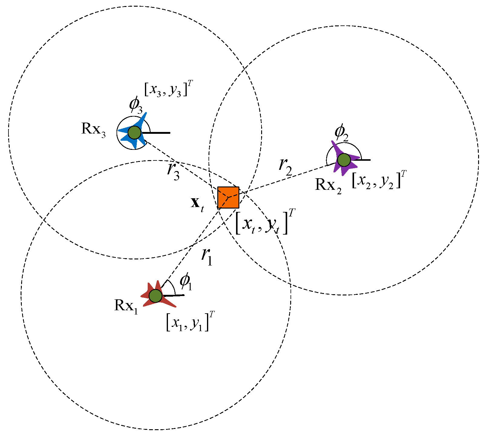
2.1. Principles of RSS

Due to the attenuation of electromagnetic signals as they propagate in space, the attenuation model of the electromagnetic signal is first constructed and the corresponding parameters are determined. Then, according to the strength of the signal received by the platforms in different positions, the position of the target can be calculated. This is the principle of received signal strength (RSS) [21,22,23,24].

Therefore, it is only necessary to obtain the strength of the signal received by each platform and the location parameters of each platform, and then passively locate the target by using RSS, as shown in Figure 1.

In Figure 1, the target radiates electromagnetic signals and its coordinates are R_t = [x_t, y_t]^T. The three platforms Rx₁, Rx₂, and Rx₃ receive radiation signals. Combined with the constructed signal attenuation model, the distance r_i between the target to be located and each detection platform can be obtained. The RSS location equation is:

$$\{\begin{array}{c}\sqrt{{(x_t-x_1)}^2+{(y_t-y_1)}^2}=r_1\\ \sqrt{{(x_t-x_2)}^2+{(y_t-y_2)}^2}=r_2\\ \sqrt{{(x_t-x_3)}^2+{(y_t-y_3)}^2}=r_3\end{array}$$

(1)

By solving Formula (1), the RSS envelope of each receiving platform in Figure 1 can be obtained. The place where the three circles overlap each other in Figure 1 is the area where the target is located.

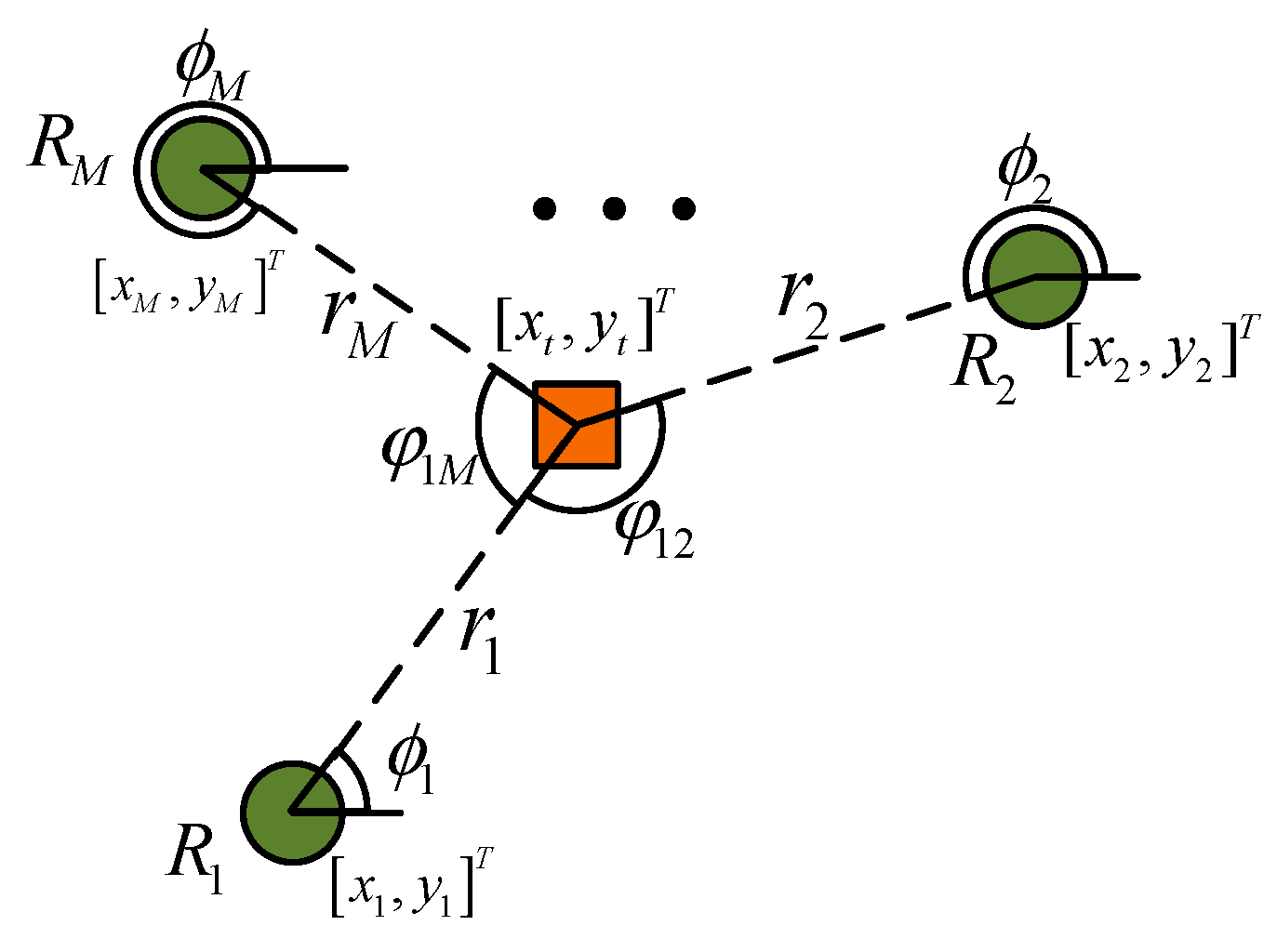
2.2. Measurement Model

This section builds a measurement model for the passive location of targets by UAV swarms. The positioning target studied in this paper was located on the ground or sea, and the height was set to zero. It was also assumed that the UAV flies on the same altitude plane. Therefore, the positioning of this article did not consider the issue of height.

Assuming that there are M UAVs in the UAV swarm, the positional parameters and spatial relationship between the UAV swarm and the target are shown in Figure 2.

The location of the target is R_t = [x_t, y_t]^T. The position and velocity of the i-th UAV are R_i = [x_i, y_i]^T and Rv_i = [vx_i, vy_i]^T, I = 1, 2, …, M, respectively. The connecting line between the drone and the target has an included angle ${\varphi }_i$ with the x-axis. The distance from the target is r_i = ||R_i − R_t||₂, and the angle between any two UAVs and the target is φ_ij, j = 1, 2, …, M.

The attenuation model of the signal in the atmosphere is:

$$p_s=p_o-10{\gamma }_i{\log }_{10}{d}_i$$

(2)

where p_o is the equivalent radiated power of the target-radiated signal. That is, the product of the target-radiated power and the antenna gain. As these two parameters are not the concern of the research in this paper, they are not introduced in detail here. γ_i is the attenuation factor of the electromagnetic wave, and di is the length of the signal propagation path. This paper assumed that the signal is not refracted. That is, di is the distance r_i between the UAV and the target [25]. Then, the signal strength p_s of the signal reaching the UAV receiving end can be calculated by Formula (2).

Due to the existence of electromagnetic interference and clutter in the atmosphere and the thermal noise of the system in the signal receiver, the actual signal p_ir(k) received by the receiver of the i-th UAV at time k can be expressed as:

$$p_{ir}\left(k\right)=p_{is}\left(k\right)+n\left(k\right)$$

(3)

Among them, n(k) represents the measurement error that obeys the Gaussian distribution, that is, n(k) ~ N(0, ${\sigma }_i^2\left(d_i\right)$). The error is related to the distance d_i between the targets, satisfying:

$${\sigma }_i^2\left(d_i\right)=d_i^{\alpha }{\sigma }_0^2$$

(4)

where ${\sigma }_0^2$ is a constant and is the basic unit of measure for variance. α is the path attenuation factor. According to Formulas (2)–(4) and the signal P_ir(k) received by each UAV at time k, the matrix of the received signal strength distribution of the UAV swarm can be obtained as P_r(k). The P_r(k) covariance matrix is ${\sigma }_p=\mathrm{diag}\left({\sigma }_1^2\left(k\right),{\sigma }_2^2\left(k\right),\dots {\sigma }_M^2\left(k\right)\right)$. Then, the signal received by the UAV swarm can be denoted as $P_r\left(k\right)~N\left(P_s\left(k\right),{\sigma }_p\right)$, where P_s(k) represents the estimated target position using the pure signal that reaches the UAV.

After acquiring the signal energy of each point, the distance r from the target to the sensor can be estimated according to the signal attenuation model. Since the positions of the UAVs themselves are known, the multiple circles shown in Figure 1 can then be obtained using Formula (1). The overlapping areas of the different circles are the target position.

It can be seen that positioning accuracy is related to the accuracy of the signal attenuation model. The attenuation characteristics and corresponding parameters of the signal attenuation model are accurate, and the distance between the UAV and the target can be estimated well. Otherwise, the error is large. Scholars have conducted in-depth research on this and constructed a variety of attenuation models to further ensure the accuracy of distance estimation.

2.3. A Optimization Criterion

CRLB represents the theoretical limit of the error estimation performance when making unbiased estimates. In practice, CRLB can be obtained by calculating the inverse matrix of the FIM.

Evidently, the performance of CRLB is highly correlated with the accuracy of the measured parameters. The more precise the measurement, the lower the error. As shown in Figure 2, the measurement parameters obtained by the UAV about the target are highly correlated with the spatial distribution of the UAV swarm. That is, a different spatial distribution corresponds to a different CRLB. Therefore, based on CRLB, this paper optimized the trajectory of the UAV swarm to achieve the efficiency of the passive location of moving targets.

Since CRLB is in matrix form, it is not easy to use in conventional applications. Scholars have proposed the A optimization criterion for CRLB whose physical meaning is to minimize the mean square error (MSE).

The A optimization criterion can be expressed as:

$$F_A=\arg \min \left[tr\left(CRLB\right)\right]=\arg \min tr\left(J^{-1}\right)$$

(5)

where J represents the FIM of the measurement matrix, and −1 represents the inverse of this matrix. Then, J⁻¹ is CRLB.

3. Configuration Optimization Method for the Passive Location of Moving Target

3.1. Passive Location Methods for Static Objects

The passive location of stationary targets using UAV swarms includes three processes. First, the relationship between CRLB and UAV swarm coordinates is constructed. Then, using the A criterion, the space configuration of the UAV swarm corresponding to the optimal CRLB matrix is obtained. By optimizing each subsequent moment in turn, the trajectory of each UAV in the cluster can be obtained.

Assuming that the position of the target is R_t = [x_t, y_t]^T and the measurement set of M UAVs at a certain moment is P_r, FIM can be expressed as:

$$J=\left[\begin{array}{cc}{J}_{xx}& J_{xy}\\ J_{yx}& J_{yy}\end{array}\right]$$

(6)

The elements of the i-th row and the j-th column of the four matrices in Formula (6) can be expressed as:

$$\{\begin{array}{c}{J}_{xx}^{i,j}=E\left[\frac{\partial }{\partial x_{ti}}\ln (f(P_r;R_t))\frac{\partial }{\partial x_{tj}}\ln (f(P_r;R_t))\right]\\ J_{xy}^{i,j}=E\left[\frac{\partial }{\partial x_{ti}}\ln (f(P_r;R_t))\frac{\partial }{\partial y_{tj}}\ln (f(P_r;R_t))\right]\\ J_{xy}^{i,j}=E\left[\frac{\partial }{\partial y_{ti}}\ln (f(P_r;R_t))\frac{\partial }{\partial x_{tj}}\ln (f(P_r;R_t))\right]\\ J_{yy}^{i,j}=E\left[\frac{\partial }{\partial y_{ti}}\ln (f(P_r;R_t))\frac{\partial }{\partial y_{tj}}\ln (f(P_r;R_t))\right]\end{array}$$

(7)

where f(P_r; R_t) is the probability density distribution function of P_r, namely:

$$f(P_r;R_t)=\frac{1}{{\left(2\pi \right)}^{M/2}\sqrt{\det ({\sigma }_p)}}\exp \left[-\frac{1}{2}{(P_r-R_t)}^T{\sigma }_p^{-1}(P_r-R_t)\right]$$

(8)

According to the definition of FIM and as shown in Formula (7), it is necessary to obtain J_xx by continuously calculating the derivative twice. x_ti and x_tj are related, that is, the second derivative is not zero.

The horizontal axis position x_t and the vertical axis position y_t of the target coordinates are independent of each other. Being independent of each other means that both J_yx and J_xy are 0. Then, Formula (6) can be rewritten as:

$$J=\left[\begin{array}{cc}{J}_{xx}& 0\\ 0& J_{yy}\end{array}\right]$$

(9)

Similarly, since the horizontal and vertical coordinates of the target are relatively independent, the processes of obtaining J_xx and J_yy are independent of each other, and the calculation process is similar. This section analyzes J_xx.

Substituting Formula (8) into Formula (7), we obtained [26]:

$$J_{xx}^{i,j}=\frac{1}{{\sigma }_p^2}\frac{\partial P_r}{\partial x_{ti}}\frac{\partial P_r}{\partial x_{tj}}+\frac{1}{2}\frac{1}{{\sigma }_p^2}\frac{\partial {\sigma }_p}{\partial x_{ti}}\frac{\partial {\sigma }_p}{\partial x_{tj}}$$

(10)

The right side of the equal sign of Formula (10) can be regarded as the sum of two parts, which can be expressed as:

$$\begin{array}{c}{J}_{xx}^{i,j}=J_{xx1}^{i,j}+J_{xx2}^{i,j}\\ \{\begin{array}{c}{J}_{xx1}^{i,j}={\nabla }_{R_{tx}}{P}_r{}^T{\sigma }_p^{-1}{\nabla }_{R_{tx}}{P}_t\\ J_{xx2}^{i,j}=\frac{1}{2}Tr\left({\sigma }_p^{-1}\frac{\partial {\sigma }_p}{\partial x_i}{\sigma }_p^{-1}\frac{\partial {\sigma }_p}{\partial x_j}\right)\end{array}\end{array}$$

(11)

Among them, ${\nabla }_{R_{tx}}{P}_r{}^T$ is the Jacobian matrix obtained after the derivation of the target abscissa R_tx using the measured value $P_r{}^T$, which is expressed as:

$$J_{1,1}=\frac{50}{{\left(\ln (10)\right)}^2{\sigma }_0^2}{\displaystyle \sum _{i=1}^M\frac{{\gamma }_i^2\left(1+\cos 2{\varphi }_i\right)}{d_i^{a+2}}}$$

(12)

$$J_{1,2}=J_{2,1}=\frac{50}{{\left(\ln (10)\right)}^2{\sigma }_0^2}{\displaystyle \sum _{i=1}^M\frac{{\gamma }_i^2\cos 2{\varphi }_i}{d_i^{a+2}}}$$

(13)

$$J_{2,2}=\frac{50}{{\left(\ln (10)\right)}^2{\sigma }_0^2}{\displaystyle \sum _{i=1}^M\frac{{\gamma }_i^2\left(1-\cos 2{\varphi }_i\right)}{d_i^{a+2}}}$$

(14)

The meanings of the parameters in Formulas (11)–(13) are the same as those in Formulas (2)–(4), which are not repeated here.

In Formula (11), Tr represents the trace of the matrix. Then, the two partial derivatives are:

$$\frac{\partial {\sigma }_p}{\partial x_i}={\sigma }_0^2\left[\begin{array}{cccc}{d}_1^{\alpha -1}\cos {\varphi }_1& 0& \cdots & 0\\ 0& d_2^{\alpha -1}\cos {\varphi }_2& \cdots & 0\\ ⋮& ⋮& \ddots & ⋮\\ 0& 0& \cdots & d_M^{\alpha -1}\cos {\varphi }_M\end{array}\right]$$

(15)

$$\frac{\partial {\sigma }_p}{\partial x_j}={\sigma }_0^2\left[\begin{array}{cccc}{d}_1^{\alpha -1}\sin {\varphi }_1& 0& \cdots & 0\\ 0& d_2^{\alpha -1}\sin {\varphi }_2& \cdots & 0\\ ⋮& ⋮& \ddots & ⋮\\ 0& 0& \cdots & d_M^{\alpha -1}\sin {\varphi }_M\end{array}\right]$$

(16)

To further simplify Formula (11), let:

$${\beta }_i=\frac{{\alpha }^2}{d_i^2}+\frac{25{\gamma }_i^2}{{\left(\ln (10)\right)}^2{\sigma }_0^2{d}_i^{a+2}}$$

(17)

Then, J_xx can be expressed as:

$$J_{xx}=\left[\begin{array}{cc}{\displaystyle \sum _{i=1}^M{\beta }_i}+{\displaystyle \sum _{i=1}^M{\beta }_i\cos 2{\varphi }_i}& {\displaystyle \sum _{i=1}^M{\beta }_i\sin 2{\varphi }_i}\\ {\displaystyle \sum _{i=1}^M{\beta }_i\sin 2{\varphi }_i}& {\displaystyle \sum _{i=1}^M{\beta }_i}-{\displaystyle \sum _{i=1}^M{\beta }_i\cos 2{\varphi }_i}\end{array}\right]$$

(18)

Then, the corresponding CRLB can be expressed as:

$$J_{xx}^{-1}=\frac{1}{\det (J_{xx})}\left[\begin{array}{cc}{\displaystyle \sum _{i=1}^M{\beta }_i}-{\displaystyle \sum _{i=1}^M{\beta }_i\cos 2{\varphi }_i}& -{\displaystyle \sum _{i=1}^M{\beta }_i\sin 2{\varphi }_i}\\ -{\displaystyle \sum _{i=1}^M{\beta }_i\sin 2{\varphi }_i}& {\displaystyle \sum _{i=1}^M{\beta }_i}+{\displaystyle \sum _{i=1}^M{\beta }_i\cos 2{\varphi }_i}\end{array}\right]$$

(19)

The value of the J_xx determinant can be expressed as:

$$\begin{array}{ll}\det (J_{xx})& =\frac{1}{4}\left[{\left({\displaystyle \sum _{i=1}^M{\beta }_i}\right)}^2-{\left({\displaystyle \sum _{i=1}^M{\beta }_i\cos (2{\varphi }_i)}\right)}^2-{\left({\displaystyle \sum _{i=1}^M{\beta }_i\sin (2{\varphi }_i)}\right)}^2\right]\\ & =\frac{1}{2}{\displaystyle \sum _{i=1}^M{\displaystyle \sum _{j=i+1}^M{\beta }_i{\beta }_j\left[1-\cos \left(2{\varphi }_i-2{\varphi }_j\right)\right]}}\end{array}$$

(20)

Then, according to the A optimization criterion, the objective function can be expressed as:

$$F_x^{opt}=\arg \min tr(J_{xx}^{-1})=\arg \min \frac{8{\displaystyle \sum _{i=1}^M{\beta }_i}}{{\displaystyle \sum _{i=1}^M{\displaystyle \sum _{j=i+1}^M{\beta }_i{\beta }_j\left[1-\cos \left(2{\varphi }_i-2{\varphi }_j\right)\right]}}}$$

(21)

Combining Formulas (21) and (17), it can be seen that the location accuracy of the target abscissa x_t is related to the distance di between each UAV and the target. It is also related to the angle difference ${\varphi }_i-{\varphi }_j$ between any two drones.

Formula (21) only involves the estimation of the target abscissa x_t. The estimation of the target ordinate y_t is the same as x_t; thus, Formula (10) is modified as:

$$J_{yy}^{i,j}=\frac{1}{{\sigma }_p^2}\frac{\partial P_r}{\partial y_{ti}}\frac{\partial P_r}{\partial y_{tj}}+\frac{1}{2}\frac{1}{{\sigma }_p^2}\frac{\partial {\sigma }_p}{\partial y_{ti}}\frac{\partial {\sigma }_p}{\partial y_{tj}}$$

(22)

The subsequent operation process is completely similar to J_xx in the previously mentioned article and is not repeated in this article.

Since the horizontal and vertical coordinates of the targets are independent of each other, the effects of directly calculating J as well as J_xx and J_yy are equivalent. Therefore, the optimization objective function for the passive location of stationary targets is:

$$F^{opt}=\arg \min \left(F_x^{opt}+F_y^{opt}\right)$$

(23)

3.2. The Main Difference between the Location of Moving Objects and Stationary Objects

The key difference between the location of moving targets and stationary targets is f(P_r; R_t) in Formula (8), that is, the probability density distribution function of the target position changes in different trends with the location of the target.

In the process of locating a stationary target, since there is no prior information as a support, the target obeys a uniform distribution on the x-axis and y-axis. That is, f(P_r; R_t) obeys an equal probability distribution on the abscissa and ordinate axes. Then, as the location progresses, it obeys the Gaussian distribution.

In the process of locating the moving target, as the location continues, the coordinates of the target in the next moment does not obey a uniform distribution on the entire coordinate axis. Instead, the f(P_r; R_t) of the target position in the next moment should be derived by combining the existing multiple location results and the target movement trend.

That is, the main difference between the location of moving objects and stationary objects is that, in the process of location moving objects, the probability density f(P_r; R_t) of the spatial distribution of the objects should be adjusted in real time.

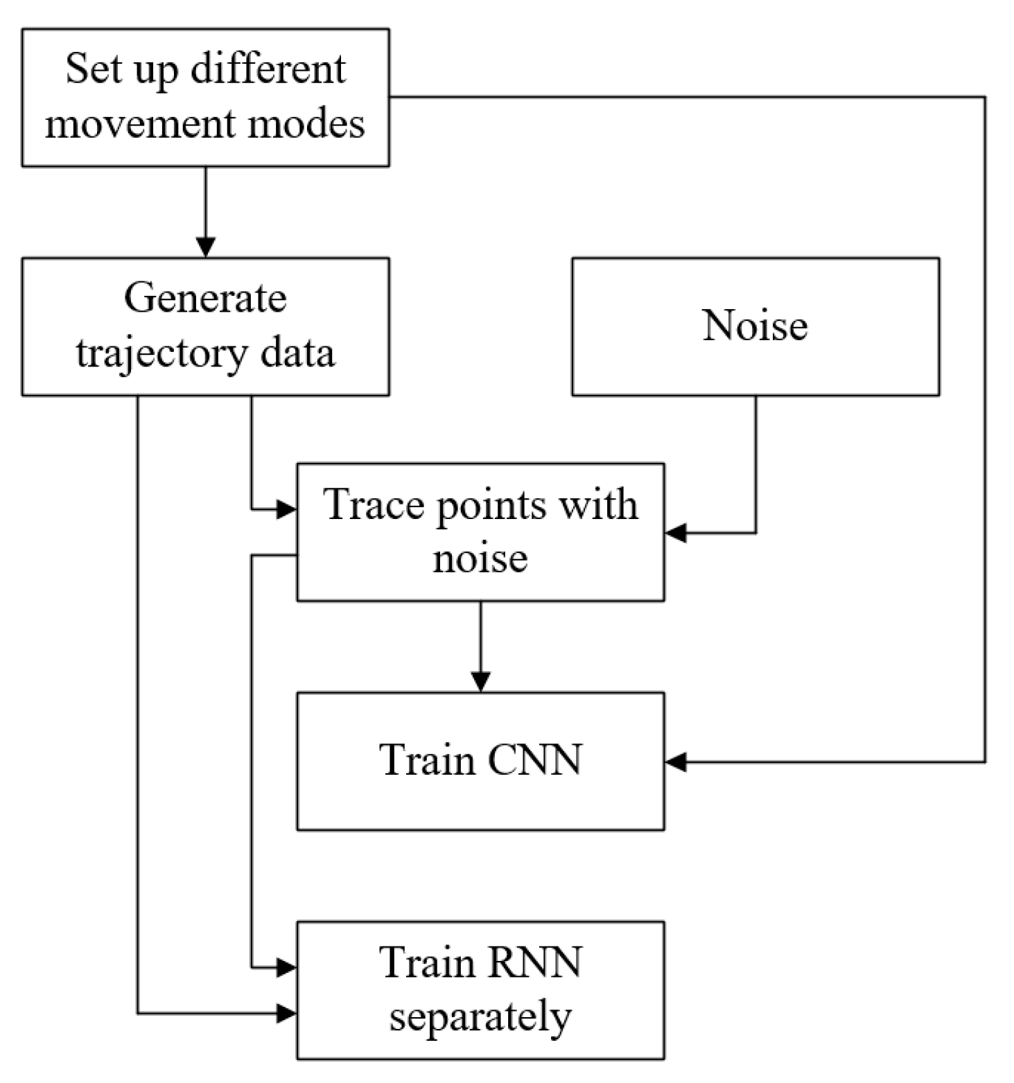
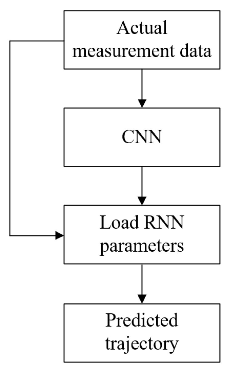
3.3. Probability Distribution Determination Method Based on Deep Combinatorial Network

With the continuous location, the probability distribution characteristics and parameters of f(P_r; R_t) continue to change. However, due to differences in target characteristics and intent, it is impossible to obtain a common or unambiguous expression. Therefore, this section adopts an approach based on deep combinatorial networks. By training the deep combinatorial network, a large number of iterations predicts the position of the target in the next moment. Thus, probability is replaced by frequency, and the probability density function of the spatial distribution of the target is quantified.

In order to improve the accuracy of target location prediction, the motion state of the target must be identified first. The discrimination of the motion state is essentially a classification problem. Because the types of target motion patterns are fixed, that is, the total number of categories for classification is determined, this paper utilized convolutional neural networks (CNN) to determine the motion state. The target trajectory prediction is actually the prediction of the time series. A recursive neural network (RNN) has good processing ability for time-series data.

Therefore, this section uses CNN and RNN to build a combined network architecture to achieve target intent recognition and trajectory prediction. The network is divided into two parts: offline training and online application; offline training is shown in Figure 3.

The specific process of offline training in Figure 3 can be described as:

Step 1: Set the target motion state and generate trajectory parameters in combination with performance indicators. Then, data corresponding to different motion states are generated. It is assumed that the target motion state includes three types: Constant Velocity (CV), Constant Acceleration (CA), and Constant Turn Rate (CT).

Step 2: Combine the characteristics of the environment and noise to generate the corresponding noise.

Step 3: Train the CNN for recognizing motion states.

Step 4: Train the RNN network parameters for predicting the trajectories of different motion states.

Through the above process, the CNN and RNN network training can be achieved.

Among them, Step 4 trains the corresponding network parameters according to the different motion states of the target, which can improve the applicability of the network and further improve the prediction accuracy.

The specific process of online application in Figure 4 can be described as:

Step 1: Use the RSS passive location method to obtain the trajectory parameters of the target. Input it into the CNN to identify the motion state of the target.

Step 2: According to the identified motion state, select and load the corresponding RNN network parameters.

Step 3: Input the trajectory parameters of the target into the RNN to obtain the predicted trajectory points of the target.

To date, the single prediction of the target trajectory using the deep combination network has been achieved.

The core purpose of constructing a combined network is not to accurately predict the position of the target, but to obtain f(P_r; R_t) in Formula (8). When used online, step 3 is repeatedly executed to obtain the predicted values of the multiple sets of target positions. Frequency is used instead of probability, as f(P_r; R_t) of the target in the next moment.

This way of obtaining f(P_r; R_t) is not limited by the probability density distribution function and corresponding parameters. At the same time, it does not require sufficient professional knowledge and mathematical skills to obtain the probability density distribution function of the target in the next moment. This method is easy to operate and the results are more accurate.

At the same time, this strategy has another advantage. In practical situations, environmental noise is generally a mixture of multiple different parameters and distribution types of noise, and has time-varying characteristics. However, it is impossible to obtain the type and corresponding parameters of each noise in this mixed noise. This also leads to actual noise being much more complex than theoretical noise and inability to build a theoretical model of environmental noise. Furthermore, subsequent quantitative analysis and formula derivation cannot be carried out. The CNN network in this paper can construct noise distribution based on actual measured parameters. The CNN network can be trained using the previously measured target and noise measurements. This research can greatly improve the accuracy of trajectory recognition in complex noise backgrounds.

Although deep learning can be used to predict the position of the target, it is still necessary to combine the FIM to optimize the spatial position of the UAV and improve the passive location accuracy. Therefore, its essence is still an NP-hard problem, and it is difficult to obtain an analytical solution.

Therefore, this paper improved the particle swarm algorithm and optimized the spatial position and trajectory of the UAV to improve the accuracy of the passive location of moving targets. There are two main reasons for using the PSO algorithm in this article.

The first reason is that it is difficult to obtain the expression of the parameter f(P_r; R_t) through theoretical derivation. Due to such constraints, even if f(P_r; R_t) is set, deriving an analytical solution is extremely difficult and not universal. Therefore, this article used intelligent optimization algorithms to solve it.

The second reason is that, compared to many other intelligent optimization algorithms, the PSO algorithm is recognized as being the fastest. The in-depth research that has been conducted on PSO is sufficient to ensure the effectiveness of PSO and, also due to the extensive research on PSO, its algorithm has good stability.

4. Improved Particle Swarm Optimization Algorithm

4.1. Particle Swarm Optimization Algorithm and Its Shortcomings

Particle swarm optimization (PSO) [27,28] was established by observing the predation characteristics of birds. The algorithm is simple to operate, efficient in searches, and has been widely used in many fields.

Assume that the dimension of the search space to be optimized is D, the total number of particles is N, and the total number of search iterations is T. Then, the updated iterative formula for optimization is:

$$v_{id}^{t+1}=\omega v_{id}^t+c_1{r}_1\left(p_{ibest}^t-x_{id}^t\right)+c_2{r}_2\left(p_{gbest}^t-x_{id}^t\right)$$

(24)

$$x_{id}^{t+1}=x_{id}^t+v_{id}^{t+1}$$

(25)

where $v_i^t=\left(v_{i1}^t,v_{i2}^t,\cdots ,v_{iD}^t\right)$ represents the set of velocities of the i-th particle in each dimension during the t-th iteration; $x_i^t$ represents the set of particle position, i = 1, 2, …, N, d = 1 , 2, …, D, t = 1, 2, …, T; ω is the inertia coefficient; c₁ and c₂ are learning factors; and r₁ and r₂ are random numbers uniformly distributed between [0, 1]. $p_{ibest}^t$ and $p_{gbest}^t$ are the best positions in individual history and population history, respectively.

Then, the fitness function corresponding to the particle position is calculated. The better the fitness, the better the position of the particle. All particles adjust their speed direction and move towards a better position by comparing their fitness functions with that of other particles.

The above is the core formula and basic principle of the PSO algorithm. It can be seen that the PSO algorithm only needs to adjust the flying speed of the particles to achieve optimization.

Although PSO can easily achieve the local optimal solution, especially for typical multimodal functions, its search efficiency is limited. This is due to the fact that particles are easily influenced by other particles. Some particles are affected by other better particles when they do not search a certain area completely. All move towards the position of the optimal particle at this stage, resulting in premature maturity.

If it is possible to conduct a complete and thorough search of each area, a global comparison can be established. Or during the movement, a detailed search for the area within the movement track can be performed. This can reduce the possibility of falling into a local optimum. Therefore, this paper constructs a time-period-based hierarchical PSO improvement strategy to improve the search performance of PSO.

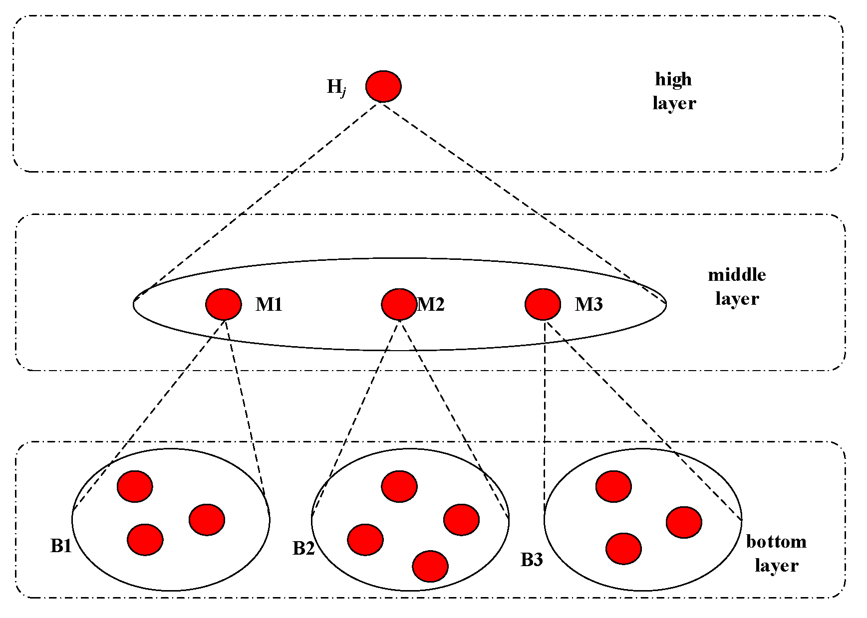
4.2. Time-Period-Based Hierarchical PSO

The architecture of the time-period-based hierarchical PSO is shown in Figure 5.

The core idea of layering is to construct three groups according to the distribution of particles: bottom layer, middle layer, and high layer. The bottom layer is explored in real time, and after interaction, the fitness function is compared to obtain the middle and high layers. The bottom layer of each group only interacts with the group, which ensures that an area is fully searched. At the same time, the best bottom layer data in this group are used as the middle layer. Then, the middle layer interacts occasionally, which balances the contradiction between the global and local searches. Afterwards, the middle and high layers guide the work of the lower layers, and the upper layers of different ethnic groups occasionally interact, thereby changing the movement pattern.

In the above discussion, how the particles are grouped and how often the particles between the middle and high layers exchange information seriously affect the algorithm performance. For this reason, it is introduced in detail later.

4.3. Particle Grouping Strategy

First, the initial population is randomly generated, and the initial position of each particle is obtained. Particles are grouped using the hierarchical clustering method. Hierarchical clustering method combines particles with similar distances into a group. In this way, particles that are close to each other can be clustered, and the result is shown in Figure 6.

The relationship between particles can be directly seen from Figure 6. Then, the number of groups is set, and the particles in the group are obtained. As shown in Figure 6, using the hierarchical clustering method, the result obtained is a typical binary tree structure. This structure is more intuitive. The red and blue lines are the grouped lines. If set to four groups, the particles below the red line become a group according to the cross-linking relationship of the grouping. The above is the process of grouping particles.

The hierarchical clustering method is a mature algorithm, and as there is a corresponding code in MATLAB, it is not repeated in this article.

After that, the particles start to be optimized. In the initial stage, the fitness function corresponding to each particle position is calculated. Then, a comparison within the group is performed to obtain the optimal particle within the group. That is, $p_{Mbest}^t$ is the best particle of the bottom layer, and it also becomes the particle of the middle layer. Afterwards, each middle-layer particle is compared to obtain the position $p_{Hbest}^t$ of the optimal particle of the group, that is, the high-level particles in Figure 5. Then, Formula (24) can be modified as:

$$v_{id}^{t+1}=\omega v_{id}^t+c_1{r}_1\left(p_{ibest}^t-x_{id}^t\right)+c_2{r}_2\left(p_{Mbest}^t-x_{id}^t\right)+c_3{r}_3\left(p_{Hbest}^t-x_{id}^t\right)$$

(26)

The parameter definitions in Formula (26) are the same as those in Formula (24), and are therefore not repeated here.

It can be seen from Formula (26) that the improved PSO is less affected by the global optimal solution. At the same time, each ethnic group searches for the optimal solution within its own territory as much as possible. This enables the adequate exploration of multiple regions. Occasional high-level interactions between groups can ensure that each group moves toward the optimal solution within the group. Ultimately, the possibility of the premature maturity of the PSO algorithm is reduced.

4.4. Time Period

The frequency of interaction between particles in the middle layer affects the direction of particle optimization. Therefore, this paper constructs a pattern of time periods to optimize the interaction frequency of the middle layer.

Assuming that the update times of the middle and high particles are t_M and t_H, respectively, that is, the middle layer optimal is updated only after every t_M iterations, Formula (26) is further modified as:

$$\begin{array}{ll}{v}_{id}^{t+1}& =\omega v_{id}^t+c_1{r}_1\left(p_{ibest}^t-x_{id}^t\right)+\frac{\mathrm{mod}\left(t,t_M\right)}{t_M}{r}_2\left(p_{Mbest}^t-x_{id}^t\right)\\ & +\frac{\mathrm{mod}\left(t,t_H\right)}{t_H}{r}_3\left(p_{Hbest}^t-x_{id}^t\right)\end{array}$$

(27)

where mod(a,b) is the remainder operation, that is, the remainder obtained after dividing a by b.

In Formula (27), when the mod operation result is small, it means that the corresponding optimal value has just been updated. At this time, it is more focused on letting the particles search in their respective areas to obtain a better $p_{ibest}^t$ for subsequent updates. As the search progresses, the mod results gradually increase, and the particles move closer to the local optimum. It is ensured that, before the next update of the local optimal value, the particle performed a more comprehensive search for the region where it is located, thereby reducing the possibility of falling into the local optimal value.

However, as the search progresses, particles within a group do not always belong to the same group. Instead, they regroup after multiple searches. This ensures a comprehensive search of the area. Therefore, in this paper, after every t_G search, all particles were regrouped according to the hierarchical clustering method in the previous section to improve the search efficiency.

The idea of the time period is borrowed from the clock model. That is, important parameters, such as the hour hand, should be updated slowly. Exploratory particles, such as the minute and second hands, should be updated faster. In this way, the effective search for the full dimension is better achieved, and the possibility of falling into a local optimum is reduced.

To sum up, this section improves the PSO algorithm by designing the particle grouping architecture and building the time period.

4.5. Algorithm Complexity Analysis

Due to the few parameters involved, the PSO algorithm has a significantly better optimization speed than other intelligent algorithms. Therefore, the improvement of the PSO algorithm should not affect its algorithm speed as much as possible. Therefore, this section analyzes the computational complexity of the improved algorithm to ensure that the speed of the algorithm does not drop significantly.

In terms of iterative update strategy, comparing Formulas (24) and (27), it can be seen that the original PSO considers the influence of individual historical optimal and global optimal on particle velocity. The improved PSO increases the impact of local optima on the speed. The amount of calculation becomes 1.5 times the original, but only the subtraction operation is performed without changing the complexity of the algorithm.

In terms of coefficients, the improved algorithm adjusts the learning factor c1 to mod operation. This operation is linear, and only needs to be performed once per iteration and the result recorded. That is, in each iteration, only one operation is performed. At the same time, subsequent particles directly use this result without repeating the calculation. The added computation has little impact compared to iterative operations.

At the level of algorithm architecture, in each iteration process, the original PSO algorithm compares the fitness functions of all particles. Thereby, the maximum value among the N fitness functions is obtained. In the improved PSO algorithm, due to the design of the time period, although the comparison is also required, the comparison within the group is mainly performed. Compared with the global comparison of the original PSO algorithm, the computational complexity of the improved PSO algorithm is significantly reduced. Although the improved algorithm also involves global comparison, due to the hierarchical structure and time period, the fitness function and the number of comparisons involved in this comparison are significantly lower than the global comparison of the original algorithm.

In the improved algorithm, the hierarchical clustering method is used to group the particles. This method needs to calculate the distance matrix between particles and then classify them according to the distance. However, due to the design of the time period, regrouping is performed only once after t_G searches. Compared with the original algorithm, each particle needs to update the fitness function corresponding to the calculation, and the increased calculation amount of the improved algorithm is very small.

To sum up, the time-period-based hierarchical PSO improvement strategy constructed in this paper only approximately increased the amount of computation to 1.5 times that of the original PSO, without changing the algorithm’s complexity. Therefore, the improved algorithm still retains the efficient characteristics of PSO.

5. Passive Location Algorithm Flow of the Moving Target Based on Improved PSO

5.1. Objective Function

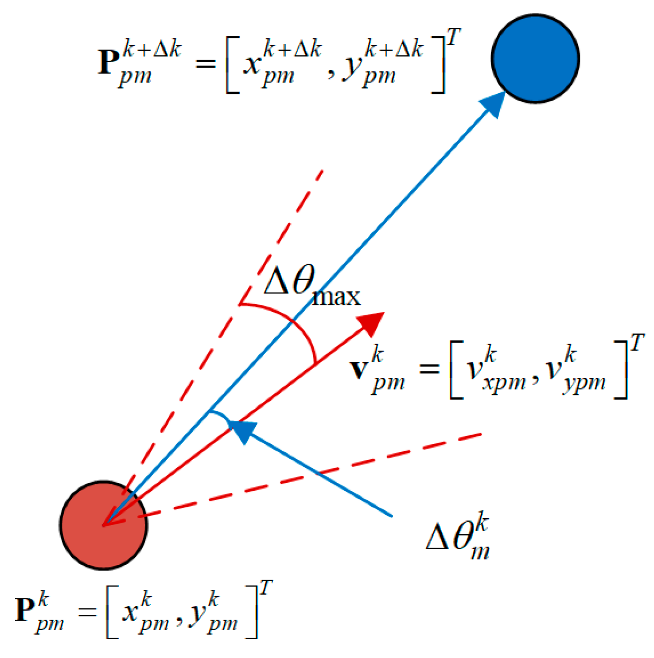
Using UAV swarms to locate moving targets is an asymptotically optimal process. Therefore, not only the location effect in the present moment, but also the subsequent impact of the decision in the present moment, should be considered. In this way, the best location effect can be achieved at a faster speed.

Assuming a time k, the subsequent motion state of the UAV swarm and the target is shown in Figure 7.

The coordinate of the i-th UAV in our UAV swarm is x_i(k) and the target coordinate is R_t(k).

At this time, the model predictive control (MPC) method was adopted. That is, the optimization method of predicting H steps and executing one step was adopted. On the basis of Formula (23), the objective function is adjusted as:

$$F{H}^{opt}=\arg \min {\displaystyle \sum _{i=0}^{H-1}{\gamma }^i{F}^{opt}\left(k+i\right)}$$

(28)

where γ is the decay factor. The MPC method used in Formula (28) is relatively mature, and is not repeated in this paper.

5.2. Constraints

Constraints mainly include individual motion constraints and obstacle avoidance constraints, as well as cluster communication constraints and collision avoidance constraints.

It was assumed that the motion state of the UAV is at k and the next moment, that is, the motion state at the moment k + Δk, as shown in Figure 8.

The position and speed of m-th UAV at time k are $P_m^k=[x_m^k,y_m^k]$ and ${\mathrm{v}}_m^k=[v_{xm}^k,v_{ym}^k]$. Taking it as the initial condition, it was optimized to obtain the position and velocity in the next moment as $P_m^{k+\Delta k}=[x_m^{k+\Delta k},y_m^{k+\Delta k}]$ and ${\mathrm{v}}_m^{k+\Delta k}=[v_m^{k+\Delta k},v_m^{k+\Delta k}]$, respectively. The corresponding relationship is shown in Figure 8. Then, the motion constraints should be satisfied, namely:

$$\{\begin{array}{c}{P}_m^{k+\Delta k}=P_m^k+v_m^k\Delta k\\ {\Vert P_m^{k+\Delta k}-P_m^k\Vert }_2\le {\Vert v_m^k\Vert }_2\Delta k\end{array}$$

(29)

where ${\Vert \Vert }_2$ means to take the 2-norm. The relationship between the speeds is:

$$v_m^{k+\Delta k}=v_m^k+\Delta v_m^k$$

(30)

where $\Delta v_m^k$ is the value of the velocity change, which should satisfy:

$$\{\begin{array}{c}{\Vert \Delta v_m^k\Vert }_2\le \Delta v_{\max }\\ v_{\min }\le {\Vert v_m^{k+\Delta k}\Vert }_2\le v_{\max }\end{array}$$

(31)

That is, the speed and the amount of speed change cannot exceed their allowable limit.

Similarly, the change amount $\Delta {\theta }_m^k$ of the UAV direction can be calculated according to the velocity vector at two moments, which should satisfy:

$$\Delta {\theta }_m^k\le \Delta {\theta }_{\max }$$

(32)

where | | represents the absolute value.

The above are the motion constraints that the UAV should meet.

The remaining three constraints are mainly reflected in the spatial distance. Among them, the individual obstacle avoidance constraints are mainly that the minimum distance between the UAV and the obstacle during the entire flight process cannot be lower than the set safe distance.

The communication constraints of the swarm require that, for any UAV, there is at least one UAV whose distance to the UAV is less than the set communication distance.

The collision avoidance constraint is the opposite, requiring that the distance between any two UAVs is not lower than the set collision avoidance distance.

The above three constraints are relatively simple and are not described in detail in this article.

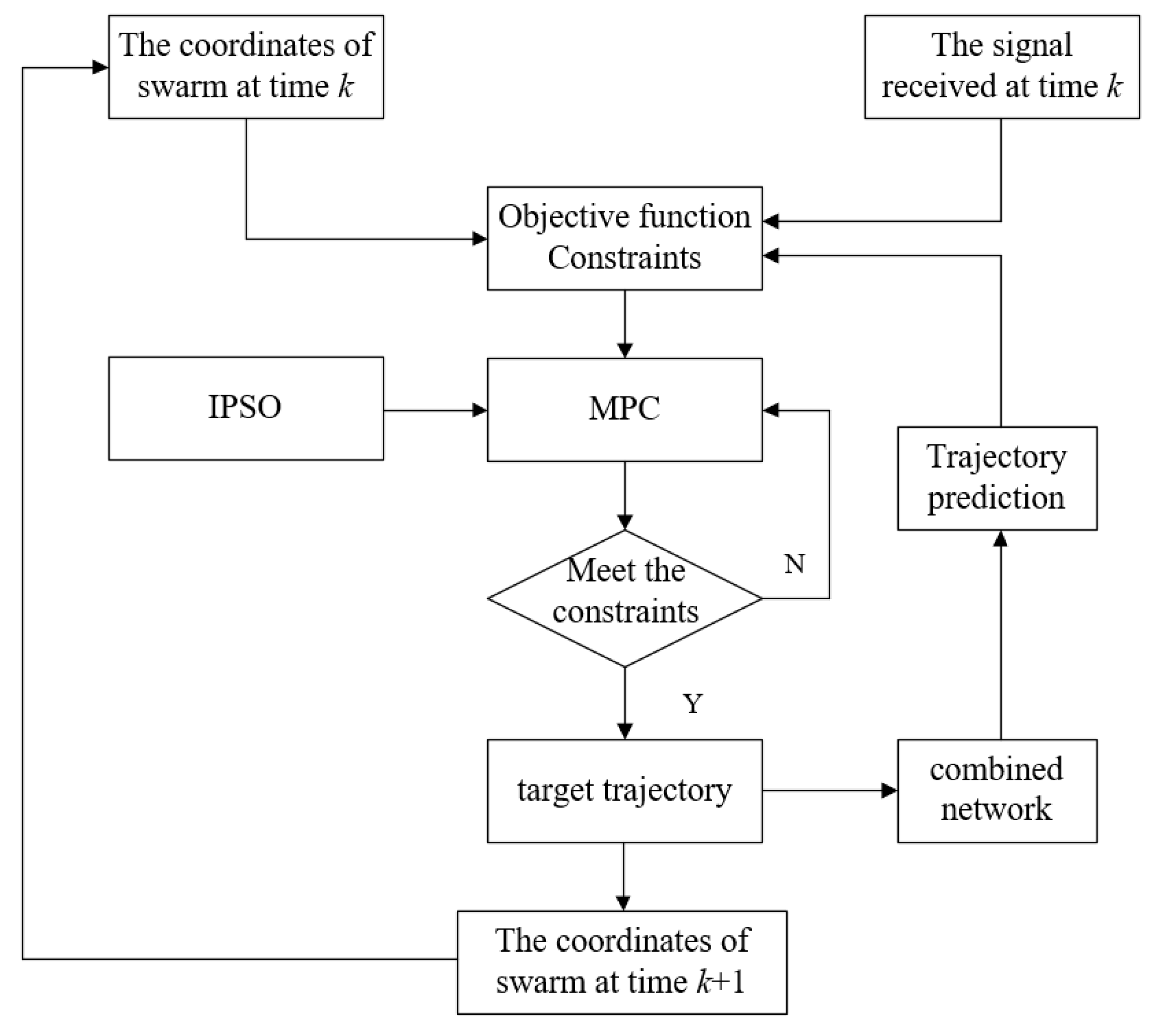
5.3. Algorithm Optimization Process

In order to achieve the passive location of moving targets, the construction algorithm flow is shown in Figure 9.

The algorithm flow of Figure 9 can be described as:

Step 1: Obtain the position of each UAV in swarm at time k and the signals received by each platform.

Step 2: Construct the objective function shown in Formula (28) and construct the corresponding constraints. Use the improved PSO algorithm and MPC for optimization.

Step 3: Judge whether the result satisfies the constraint conditions; if not, return to Step 2; if it is satisfied, execute Step 4.

Step 4: Construct a time series of the location points obtained at this time and the previous five moments. It is fed into the combined network to predict the target trajectory. The predicted result is used to correct f(P_r; R_t) in Formula (8).

Step 5: Obtain the optimal coordinates of each drone in the next moment and then update the position of the drone. Determine whether the final optimization time k is reached. If it is not reached, return to Step 1; otherwise, the optimization ends.

The above is the algorithm flow of using UAV swarm to locate the moving target.

6. Simulation and Verification

To verify the performance of the algorithm in this paper, it was assumed that the target run for 60 min, 1–20 min for CV, 21–40 min for CT, and 41–60 min for CA.

Five UAVs took off near (0,0) with a speed limit of 200 m/min and performed the cooperative passive location of the target.

The simulation environment was I7-10750H, with 2.60 GHz dominant frequency and 16 G memory, and the simulation experiment was made on a platform based on MATLAB 2020b.

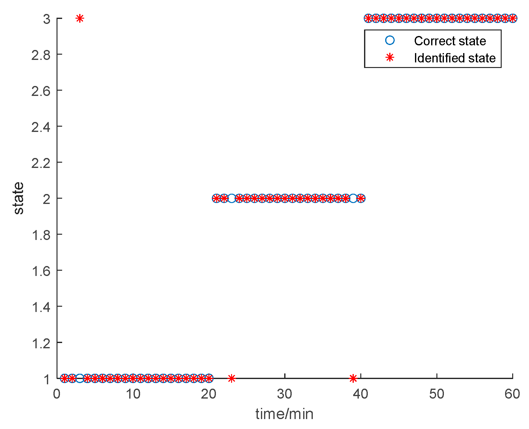
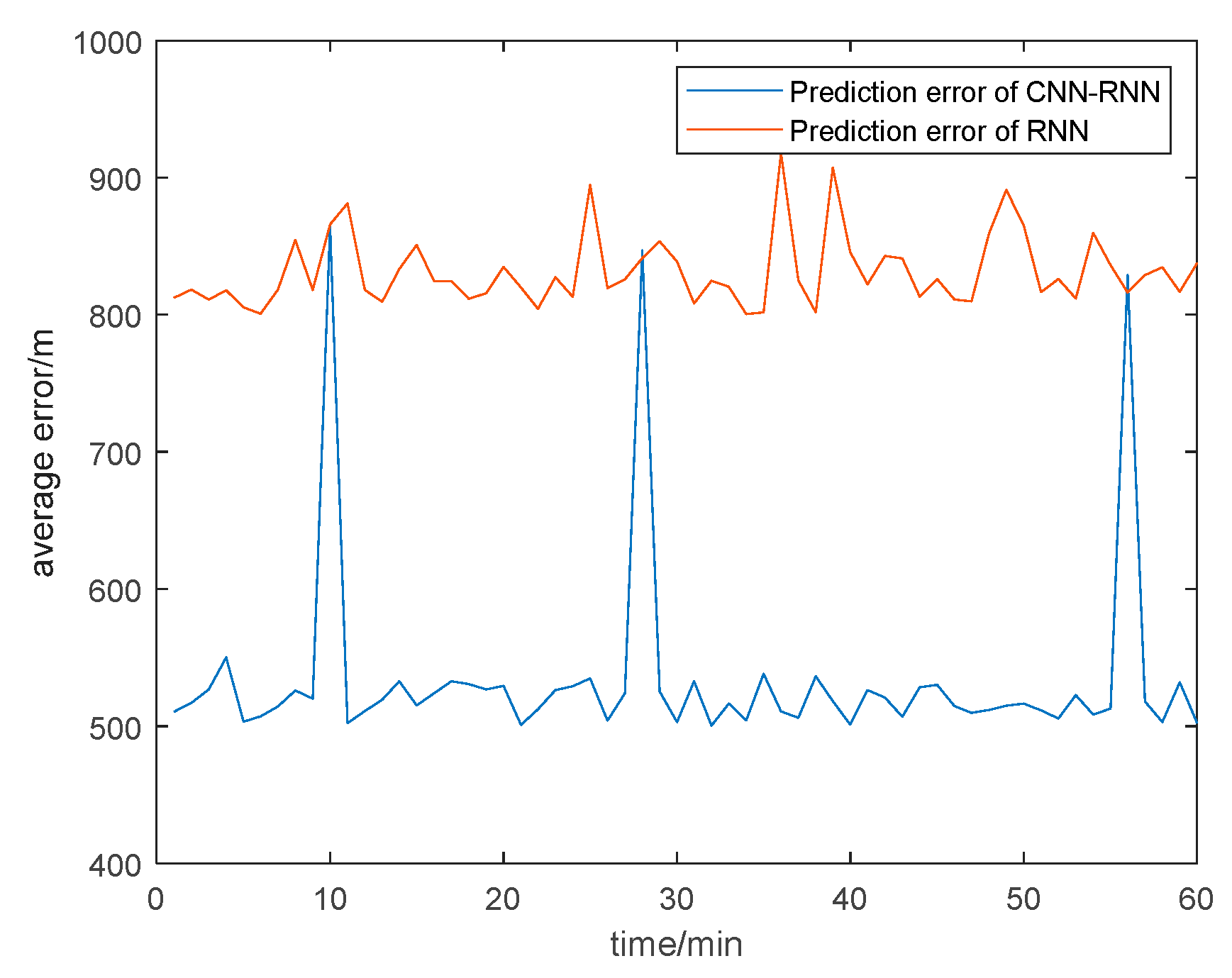
6.1. Performance Verification of Deep Networks

To verify the performance of the network built in Section 3.3, this section conducts simulation experiments on the network.

The data used to train the CNN network were the track data added with standard Gaussian white noise. At the same time, it was necessary to identify the target’s motion state in this minute; so, the training data were 60 s, which means to generate a data sequence with a length of 60 based on the above motion state and corresponding time. The output of the training was the motion state of the trajectory, namely, the three motion states of CV, CA, and CT. This article set 60 points per minute. The target movement lasted for a total of 60 min. To ensure sufficient training data, 360,000 sets of data were generated for training, and an additional 3600 sets of data were generated for testing. The test was passed when the test error was set to not less than 95%.

Since the length of the data used for training was only 60, the data were not long. Thus, the number of network layers was set to 7, that is, 5 of them were hidden layers, the learning rate was 0.3, eight neurons per layer, and the number of iterations was 2000. Comparing the algorithm with IMM-EKF [29], the result is shown in Figure 10.

From Figure 10, it can be seen that CNN has three errors and IMM-EKF has six. CNN is more accurate than IMM-EKF. This is because the basic function of CNN is recognition, and the recognition effect will increase with the increase in training data. However, the recognition effect of IMM-EKF is affected by noise, and the performance does not change with the amount of training data. Therefore, CNN is more suitable for target motion state recognition.

The data used to train the CNN-RNN composite network were input for 60 points, that is, the position of the target and the motion state identified by the CNN per second. The output was 60 track points that predict the target for the next minute. A total of 360,000 sets of data were used for training and an additional 3600 sets for testing. The training was completed after the number of iterations was reached.

Because the length of the data used for training was only 60, the number of RNN network layers was set to 8 layers, that is, 6 layers were hidden layers, the learning rate was 0.3, 8 neurons per layer, and the number of iterations was 50,000. Comparing the algorithm with the classical RNN, the result is shown in Figure 11.

As can be seen from Figure 11, the prediction results of the CNN-RNN network were generally better than that of RNN. This is because there are actually three sets of RNN networks with different parameters in CNN-RNN. That is, after the CNN identifies the target motion state, the RNN loads the corresponding parameters to perform the prediction. With more targeted networks, the results will certainly be more accurate. However, once the CNN recognizes an error, the error spikes, as shown in Figure 11.

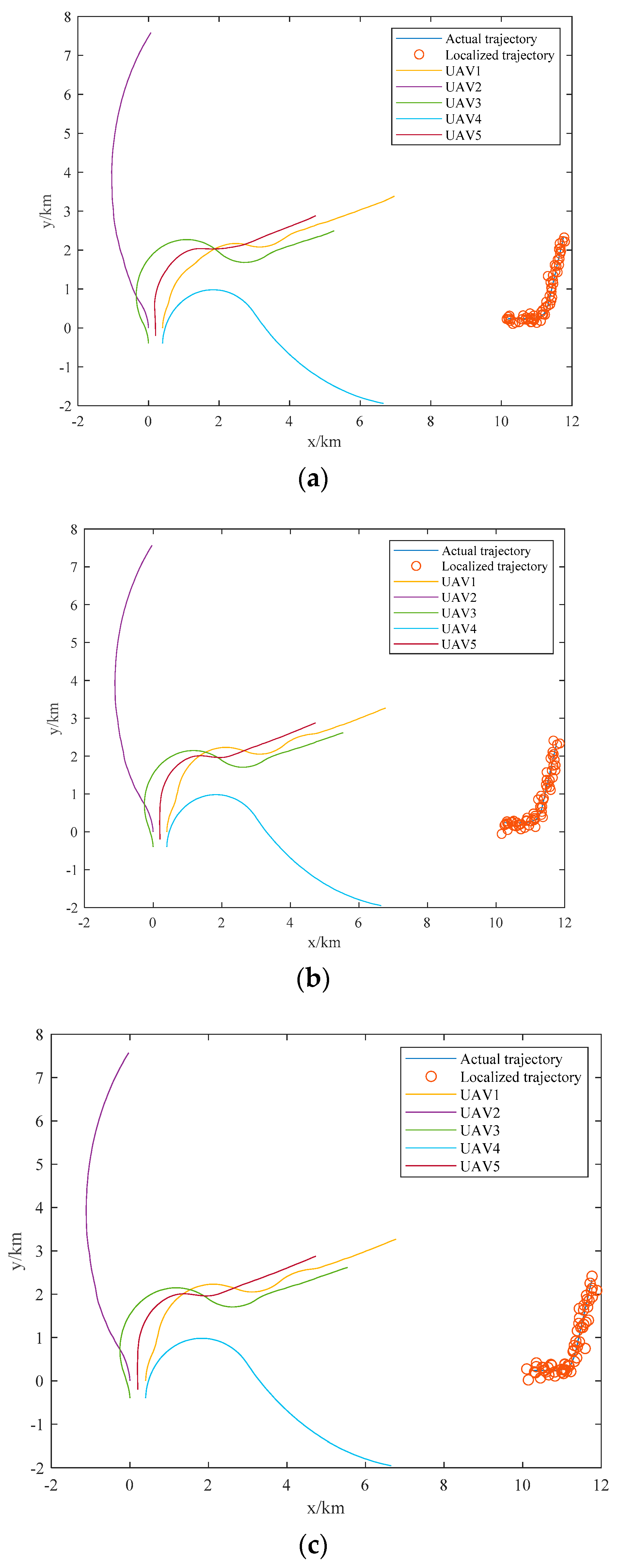
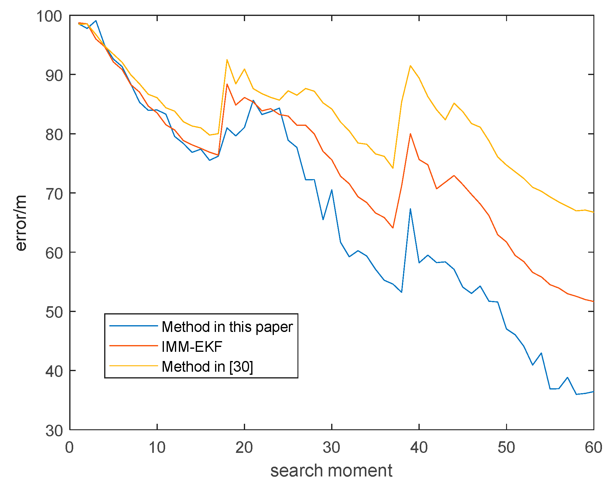
6.2. Passive Location Performance Verification and Algorithm Comparison

The algorithm in this paper, the IMM-EFK in [29], and the location method in [30] were compared, and the results are shown in Figure 12.

By comparing the three sets of results in Figure 12, it can be seen that the location points of the algorithm in this paper are more coincident with the target trajectory.

It can be seen from Figure 12b that the method of IMM-EKF has better localization accuracy. However, when the motion state of the target is converted, the IMM-EKF cannot quickly identify the change of the motion state of the target. At the same time, after identification, it is difficult to quickly establish a new tracking equation, resulting in a significant decrease in the location efficiency at this time.

Literature [30] uses Doppler rate to improve the accuracy of moving target positioning based on time delay and Doppler shift. Meanwhile, literature [30] establishes a pseudolinear set of equations by introducing some additional variables. The analytic solution for moving target positioning is given. The positioning CRLB is derived. However, by comparing Figure 12a,c, it can be seen that the positioning method in literature [30] differs from that in this paper in positioning accuracy. There are two main reasons.

The first is that, as can be seen from Figure 12c, the method in literature [30] has always had a large error. This is because the method in literature [30] does not consider the sequential nature of target motion, treating each localization as an independent localization. As a result, its positioning performance will not improve with the progress of positioning. The second reason is that the method in literature [30] does not achieve real-time planning for the trajectory of unmanned aerial vehicles, but rather provides the ultimate ideal location point distribution method. The real-time optimization is not achieved, and motion conditions such as platform motion are not considered. This results in poor performance during the positioning process.

The core reason why the algorithm in this paper is superior to other algorithms is that this paper constructs a model of cooperative passive location from the perspective of clusters. This article does not disassemble the five UAV into a “2 + 3” model, but optimizes the five UAVs as a whole. It can be seen from Figure 12a that among the 5 UAVs, 3 UAVs are flying towards the target, which is pulling in the relative distance between the cluster and the target. The 2 UAVs flew towards a wide area, increasing the observation angles of different drones. This also conforms to Formula (21), that is, the UAV swarm adjusts the distance and angle factors that affect the location accuracy.

The algorithm in this paper obtains better location performance by adjusting the distance between the cluster and the target and forming different observation angles at the same time.

In order to further quantify and compare the location performance. Under the condition that the simulation conditions remain unchanged, 30 Monte Carlo experimental simulations are carried out for each algorithm. Take the average value of the errors at each moment to obtain a comparison chart, as shown in Figure 13.

As can be seen from Figure 13, the algorithm in this paper has two obvious advantages over other algorithms. One is that the MPC is involved in the algorithm in this paper, so its error decreases significantly faster than other algorithms.

The other is that the stability of the algorithm in this paper is stronger. When the motion state of the target changes, it is difficult for each algorithm to judge the change in the state at the first time, so there is a sudden change in error in Figure 13. By comparison, it can be seen that, because the algorithm in this paper uses a combined network, the error is less affected. At the same time, the algorithm also stabilizes faster.

To further compare the effectiveness of the positioning methods, this section counts the positioning time of 30 Monte Carlo experiments of the above three methods. The results are shown in

Table 2. Comparison of time consumption of the three positioning algorithms.

Time Consumption	Algorithm in This Paper	IMM-EKF	Method in [30]
Average total time	163.26	205.81	732.42
Average time for each point	2.71	3.43	12.21

.

As can be seen from Table 2, the algorithm in this paper is superior to the other two algorithms in terms of efficiency. This is because, when using IMM-EKF to determine the motion state of a target, it is necessary to calculate the probability of the target’s motion state in the next moment based on its previous motion trajectory. The algorithm in this paper only needs to input the trajectory into the trained network, and can directly predict the position of the target in the next moment, which is faster.

The method in [30] provides an analytical solution, which can intuitively see the relationship between factors affecting the target’s positioning accuracy and quantification. However, in the solution process of [30], it involves performing inverse operations on a large number of matrices, Which seriously affects the speed of the algorithm. Therefore, it takes a long time.

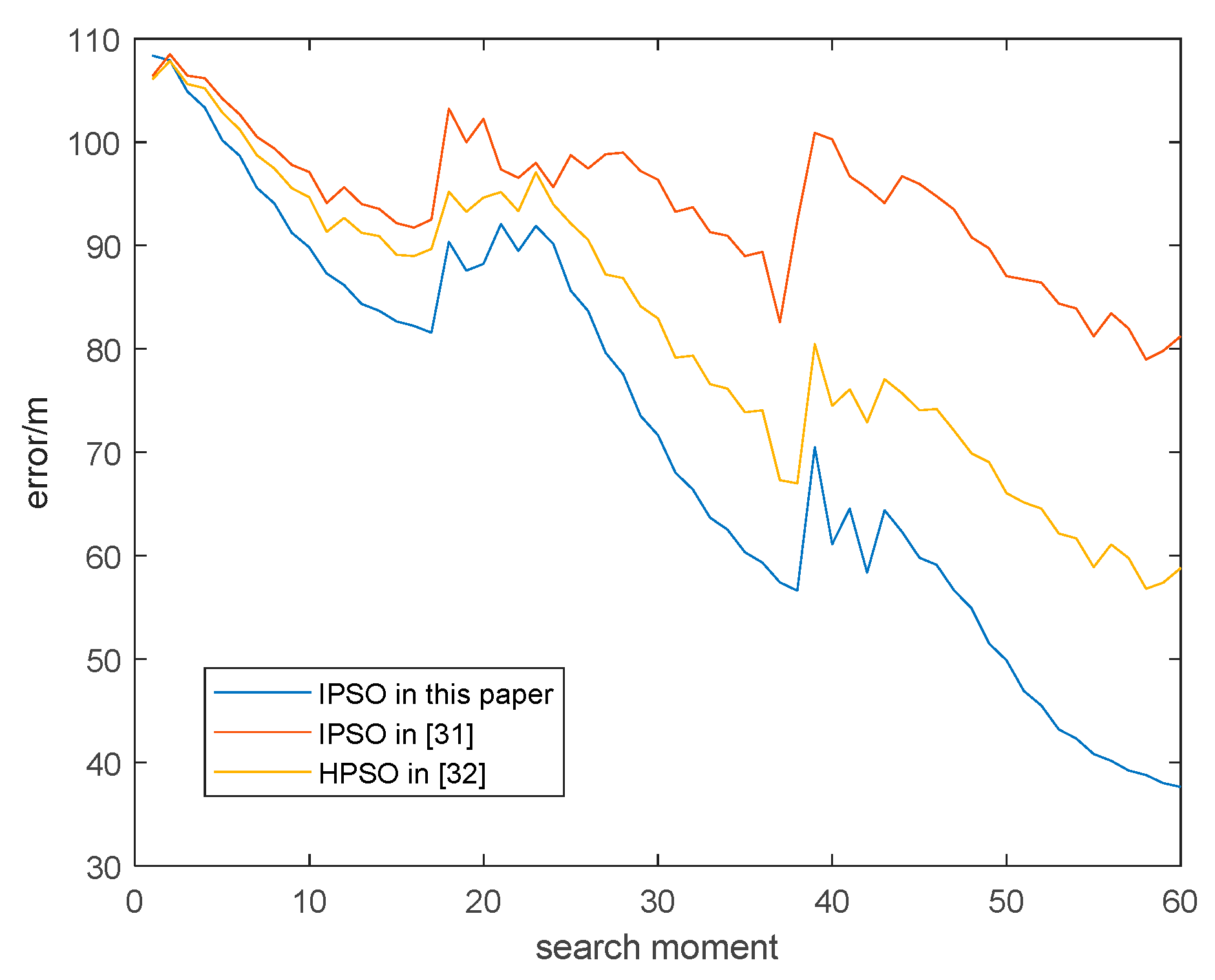
6.3. Optimization Algorithm Performance Comparison

In order to further measure and compare the performance of the improved PSO algorithm, the improved PSO in this paper was compared with the PSO in [31] and the Holonic-PSO in [32]. The simulation conditions were the same, and 30 Monte Carlo simulations were performed to obtain a comparison chart of the mean error value, as shown in Figure 14.

It can be seen from Figure 14 that the performance of the algorithm in this paper is more stable, because the algorithm in this paper can perform a more global search and improve the algorithm efficiency.

The method in [31] is more focused on enabling PSO particles to jump out of the local optimization with maximum probability, thereby achieving global search. To achieve this goal, Formulas (5)–(7) in [31] set a method for generating approximately random search directions. This setting can reduce the possibility of falling into a local optimum, but this near-random approach has no significant effect on improving search performance.

The improvement idea of this article was inspired by [32] to group particles for search. One disadvantage of [32] is that its particle search strategy, i.e., the updated equation of particle state, is artificially adjusted. In the iterative process of [32], the first 80% of searches and the last 20% of searches use different update equations. However, in [32], a simple comparative experiment shows that the ratio of 80% to 20% is better, without indicating whether it is optimal. Obviously, this ratio may vary depending on the issue.

At the same time, there is another reason why the method in this article is superior to the above two methods. What this article aimed to solve is a sequential decision-making problem. The optimization results of the previous moment affect the next moment. The positioning accuracy of the previous moment is good, providing a good initial condition for the next moment, and the positioning accuracy of the next moment will not be poor. If the positioning effect at the previous moment is poor, it will also affect the positioning at the next moment. Therefore, over time, compared to the other two methods, the effect of this article becomes better and better.

In order to further compare the performance of the algorithms, the time of the three optimization algorithms is also counted, and the results are shown in

Table 3. Comparison of the time consumption of the three optimization algorithms.

Time Consumption	Algorithm in This Paper	IPSO in [31]	HPSO in [32]
Average total time	163.26	116.46	164.47
Average time for each point	2.71	1.94	2.71

.

Through comparison, it can be seen that the algorithm speed in this article is weaker than IPSO [31], but better than HPSO [32].

The improvement of the IPSO algorithm on the search direction of the particles is still based on a random mode. Compared with the PSO algorithm, this search mode has almost no significant change in the additional computation amount generated by the PSO algorithm. Therefore, IPSO still maintains its high-speed solution efficiency. The algorithm in this paper involves further information interaction between groups and particles, with a significant increase in computational complexity. Therefore, the performance is weaker than IPSO.

Both this algorithm and HPSO [32] involve particle grouping and information interaction. However, in each iteration of the HPSO algorithm, the particle parameters at each level are updated. In this article, by designing a clock cycle, particles at different levels were updated according to the cycle, which reduces the amount of computation. This can also allow different particle populations to conduct more detailed searches of their regions.

Under the main premise of ensuring positioning accuracy, the effectiveness of the algorithm in this paper is even higher.

7. Discussion

This section mainly discusses the main contributions, application scenarios, algorithm deficiencies, and follow-up work of this article.

This paper built a passive location method for moving targets based on RSS for UAV clusters. The target probability distribution network was designed to predict the subsequent location of the target more clearly and easily. Thus, the mature static target positioning method was extended to the target positioning. At the same time, the PSO algorithm was improved in this paper. From the simulation comparison, the improved method had a good performance.

The research results can be applied in many ways, mainly using a UAV cluster to locate a target and achieve navigation without a GPS signal. UAV clusters can also be used to search and rescue people with mobile phones. Sound and electromagnetic information can be collected to build digital maps. It can also locate ships on the sea, or discover and locate concealed radar.

Although this paper has conducted some research work, there are still some limitations. Firstly, the positioning model does not take the altitude direction into account, so in practice, this study is still far from achieving more accurate applications. Secondly, although the network can suppress complex noise, its effect is limited. Finally, the real-time performance of the algorithm needs further design. The PSO algorithm cannot increase speed further, but as UAV clusters are multiple platforms, parallel computing can be considered. It is feasible to exchange computing resources for optimization time.

To overcome these shortcomings, a passive positioning model of UAV in a three-dimensional scene will be built in future research to improve the network to improve its ability of target state recognition under strong noise background. Additionally, a framework of parallel computing will be designed to test and improve the algorithm.

8. Conclusions

In this paper, the problem of improving passive location accuracy will be transformed into the problem of obtaining more target information. Based on RSS and the A criterion, a passive location method for moving objects was constructed. Firstly, the measurement model of cluster passive location was constructed. After that, the relationship between the UAV spatial position and the static target localization effectiveness was derived and constructed. Then, the difference between stationary target and moving target location was analyzed. In order to expand the scope of the application of the algorithm, the prediction of the target position was realized by designing a deep combined network. Thereby, the probability density distribution function required in the passive location process of the moving target was obtained. Considering that trajectory optimization is an NP-Hard problem and addressing the problem that the PSO algorithm easily falls into the local optimum, a layered improvement strategy based on time period was designed to improve PSO performance. Then, a passive location algorithm flow based on the improved PSO was constructed. Through simulation verification and algorithm comparison, the feasibility and performance advantages of the algorithm in this paper were highlighted.

References

1. Zou, Y.; Wan, Q. Asynchronous Time-of-Arrival-Based Source Localization with Sensor Position Uncertainties. IEEE Commun. Lett. 2016, 20, 1860–1863. [Google Scholar] [CrossRef]
2. Dang, L.; Yang, H.; Teng, B. Application of Time-Difference-of-Arrival Localization Method in Impulse System Radar and the Prospect of Application of Impulse System Radar in the Internet of Things. IEEE Access 2018, 6, 44846–44857. [Google Scholar] [CrossRef]
3. Chitte, S.D.; Dasgupta, S.; Ding, Z. Distance Estimation from Received Signal Strength under Log-Normal Shadowing: Bias and Variance. IEEE Signal Process. Lett. 2009, 16, 216–218. [Google Scholar] [CrossRef]
4. Cheng, Y.; Lin, Y. A new received signal strength based location estimation scheme for wireless sensor network. IEEE Trans. Consum. Electron. 2009, 55, 1295–1299. [Google Scholar] [CrossRef]
5. Zhao, Y.; Hu, D.; Liu, Z.; Zhao, Y. Calibrating the Transmitter and Receiver Location Errors for Moving Target Localization in Multistatic Passive Radar. IEEE Access 2019, 7, 118173–118187. [Google Scholar] [CrossRef]
6. Li, B.; Zhao, K.; Shen, X. Dilution of Precision in Location Systems Using both Angle of Arrival and Time of Arrival Measurements. IEEE Access 2020, 8, 192506–192516. [Google Scholar] [CrossRef]
7. Wei, H.; Ye, S. Comments on “A Linear Closed-Form Algorithm for Source Localization from Time-Differences of Arrival”. IEEE Signal Process. Lett. 2008, 15, 895. [Google Scholar] [CrossRef]
8. Abeywickrama, S.; Samarasinghe, T.; Ho, C.K.; Yuen, C. Wireless Energy Beamforming Using Received Signal Strength Indicator Feedback. IEEE Trans. Signal Process. 2018, 66, 224–235. [Google Scholar] [CrossRef]
9. Maric, A.; Kaljic, E.; Njemcevic, P.; Lipovac, V. Projective Approach in Determining Homogeneous Hyperspherical Geometrically-Based Stochastic Channel Model’s Statistics: Angle of Departure, Angle of Arrival and Time of Arrival. IEEE Trans. Wirel. Commun. 2020, 19, 7864–7880. [Google Scholar] [CrossRef]
10. Xu, H.; Zhang, Y.; Ba, B.; Wang, D.; Li, X. Fast Joint Estimation of Time of Arrival and Angle of Arrival in Complex Multipath Environment Using OFDM. IEEE Access 2018, 6, 60613–60621. [Google Scholar] [CrossRef]
11. Schau, H.; Robinson, A. Passive source localization employing intersecting spherical surfaces from time-of-arrival differences. IEEE Trans. Acoust. Speech Signal Process. 1987, 35, 1223–1225. [Google Scholar] [CrossRef]
12. Wang, X.; Huang, Z.; Zhou, Y. Underdetermined DOA estimation and blind separation of non-disjoint sources in time-frequency domain based on sparse representation method. J. Syst. Eng. Electron. 2014, 25, 17–25. [Google Scholar] [CrossRef]
13. Zhang, M.; Guo, F.; Zhou, Y.; Yao, S. A Single Moving Observer Direct Position Determination Method Using Interferometer Phase Difference. Acta Aeronaut. Astronaut. Sin. 2013, 34, 2185–2193. [Google Scholar]
14. Liu, Y.; Guo, F.; Yang, L.; Jiang, W. Source localization using a moving receiver and noisy TOA measurements. Signal Process. 2016, 119, 185–189. [Google Scholar] [CrossRef]
15. Xi, L.; Guo, F.; Le, Y.; Min, Z. Improved solution for geolocating a known altitude source using TDOA and FDOA under random sensor location errors. Electron. Lett. 2018, 54, 597–599. [Google Scholar]
16. Wang, G.H.; Bai, J.; He, Y.; Xiu, J.J. Optimal deployment of multiple passive sensors in the sense of minimum concentration ellipse. IET Radar Sonar Navig. 2009, 3, 8–17. [Google Scholar] [CrossRef]
17. Bishop, A.N.; Fidan, B.; Anderson, B.D.O. Optimality Analysis of Sensor-Target Geometries in Passive Location: Part 2—Time-of-Arrival Based Localization. In Proceedings of the 3rd International Conference on Intelligent Sensors Sensor Networks and Information Processing, Melbourne, VIC, Australia, 3–6 December 2007. [Google Scholar]
18. Bishop, A.N.; Fidan, B.; Anderson, B.D.O. Optimality Analysis of Sensor-Target Geometries in Passive Location: Part 1—Bearing-Only Localization. In Proceedings of the 3rd International Conference on Intelligent Sensors Sensor Networks and Information Processing, Melbourne, VIC, Australia, 3–6 December 2007; pp. 7–12. [Google Scholar]
19. Lui, K.W.K.; So, H.C. A Study of Two-Dimensional Sensor Placement Using Time-Difference-of-Arrival Measurements. Digit. Signal Process. 2009, 19, 650–659. [Google Scholar] [CrossRef]
20. Yang, B.; Scheuing, J. A Theoretical Analysis of 2D Sensor Arrays for TDOA Based Localization; ICASSP: Toulouse, France, 2006; pp. 901–904. [Google Scholar]
21. Wu, Z.; Fu, K.; Jedari, E.; Shuvra, S.R.; Rashidzadeh, R.; Saif, M. A Fast and Resource Efficient Method for Indoor Location Using Received Signal Strength. IEEE Trans. Veh. Technol. 2016, 65, 9747–9758. [Google Scholar] [CrossRef]
22. Xu, S.; Ou, Y.; Zheng, W. Optimal Sensor-Target Geometries for 3-D Static Target Localization Using Received-Signal-Strength Measurements. IEEE Signal Process. Lett. 2019, 26, 966–970. [Google Scholar] [CrossRef]
23. Vaghefi, R.M.; Gholami, M.R.; Buehrer, R.M.; Strom, E.G. Cooperative Received Signal Strength-Based Sensor Localization with Unknown Transmit Powers. IEEE Trans. Signal Process. 2013, 61, 1389–1403. [Google Scholar] [CrossRef] [Green Version]
24. Hemavathi, N.; Meenalochani, M.; Sudha, S. Influence of Received Signal Strength on Prediction of Cluster Head and Number of Rounds. IEEE Trans. Instrum. Meas. 2020, 69, 3739–3749. [Google Scholar] [CrossRef]
25. So, H.C.; Lin, L. Linear Least Squares Approach for Accurate Received Signal Strength Based Source Localization. IEEE Trans. Signal Process. 2011, 59, 4035–4040. [Google Scholar] [CrossRef]
26. Kay, S.M. Fundamentals of Statistical Signal Processing: Estimation Theory; Prentice Hall PTR: Upper Saddle River, NJ, USA, 1993; pp. 47, 73–76. [Google Scholar]
27. Zhang, B.; Zhuang, L.; Gao, L.; Luo, W.; Ran, Q.; Du, Q. PSO-EM: A Hyperspectral Unmixing Algorithm Based on Normal Compositional Model. IEEE Trans. Geosci. Remote Sens. 2014, 52, 7782–7792. [Google Scholar] [CrossRef]
28. Sun, T.; Tang, C.; Tien, F. Post-Slicing Inspection of Silicon Wafers Using the HJ-PSO Algorithm under Machine Vision. IEEE Trans. Semicond. Manuf. 2011, 24, 80–88. [Google Scholar] [CrossRef]
29. Hernandez, M.; Farina, A. PCRB and IMM for Target Tracking in the Presence of Specular Multipath. IEEE Trans. Aerosp. Electron. Syst. 2020, 56, 2437–2449. [Google Scholar] [CrossRef]
30. Yongsheng, Z.; Dexiu, H.; Yongjun, Z.; Zhixin, L. Moving target localization for multistatic passive radar using delay, Doppler and Doppler rate measurements. J. Syst. Eng. Electron. 2020, 31, 939–949. [Google Scholar] [CrossRef]
31. Mistry, K.; Zhang, L.; Neoh, S.C.; Lim, C.P.; Fielding, B. A Micro-GA Embedded PSO Feature Selection Approach to Intelligent Facial Emotion Recognition. IEEE Trans. Cybern. 2017, 47, 1496–1509. [Google Scholar] [CrossRef] [Green Version]
32. Roshanzamir, M.; Balafar, M.A.; Razavi, S.N. Empowering particle swarm optimization algorithm using multi agents’ capability: A holonic approach. Knowl. Based Syst. 2017, 136, 58–74. [Google Scholar] [CrossRef]
Figure 1. Schematic diagram of RSS location.
Drones 07 00264 g001
Figure 2. Schematic diagram of the passive location of the UAV swarm.
Drones 07 00264 g002
Figure 3. The process of offline training.
Drones 07 00264 g003
Figure 4. The process of online application.
Drones 07 00264 g004
Figure 5. Schematic diagram of the layered architecture.
Drones 07 00264 g005
Figure 6. Schematic diagram of the hierarchical clustering method results.
Drones 07 00264 g006
Figure 7. Movement situation diagram.
Drones 07 00264 g007
Figure 8. Schematic diagram of motion constraints.
Drones 07 00264 g008
Figure 9. Flowchart of the passive location algorithm for the moving target by UAV swarm.
Drones 07 00264 g009
Figure 10. Comparison of the recognition results.
Drones 07 00264 g010
Figure 11. Comparison of the average error.
Drones 07 00264 g011
Figure 12. Comparison of algorithm optimization results. (a) Optimization results of the algorithm in this paper; (b) IMM−EKF optimization results; and (c) the results of the location method in [30].
Drones 07 00264 g012
Figure 13. Comparison of average errors [30].
Drones 07 00264 g013
Figure 14. Error comparison chart [31,32].
Drones 07 00264 g014