Article

Off-Policy Deep Reinforcement Learning for Path Planning of Stratospheric Airship

1
Aerospace Information Research Institute, Chinese Academy of Sciences, Beijing 100094, China
2
University of Chinese Academy of Sciences, Beijing 100190, China
*
Author to whom correspondence should be addressed.
Drones 2025, 9(9), 650; https://doi.org/10.3390/drones9090650
Submission received: 29 July 2025 / Revised: 5 September 2025 / Accepted: 11 September 2025 / Published: 16 September 2025
(This article belongs to the Special Issue Design and Flight Control of Low-Speed Near-Space Unmanned Systems)

Abstract

The stratospheric airship is a vital platform in near-space applications, and achieving autonomous transfer has become a key research focus to meet the demands of diverse mission scenarios. The core challenge lies in planning feasible and efficient paths, which is difficult for traditional algorithms due to the time-varying environment and the highly coupled multi-system dynamics of the airship. This study proposes a deep reinforcement learning algorithm, termed reward-prioritized Long Short-Term Memory Twin Delayed Deep Deterministic Policy Gradient (RPL-TD3). The method incorporates an LSTM network to effectively capture the influence of historical states on current decision-making, thereby improving performance in tasks with strong temporal dependencies. Furthermore, to address the slow convergence commonly seen in off-policy methods, a reward-prioritized experience replay mechanism is introduced. This mechanism stores and replays experiences in the form of sequential data chains, labels them with sequence-level rewards, and prioritizes high-value experiences during training to accelerate convergence. Comparative experiments with other algorithms indicate that, under the same computational resources, RPL-TD3 improves convergence speed by 62.5% compared to the baseline algorithm without the reward-prioritized experience replay mechanism. In both simulation and generalization experiments, the proposed method is capable of planning feasible paths under kinematic and energy constraints. Compared with peer algorithms, it achieves the shortest flight time while maintaining a relatively high level of average residual energy.

1. Introduction

Stratospheric airship is a class of lighter-than-air vehicles that operate in the stratosphere and are capable of long-duration station-keeping [1,2]. They offer advantages such as low operational cost, high payload capacity, and the ability to remain aloft for extended periods. Due to their large frontal area and high drag coefficient, the motion of stratospheric airships is highly susceptible to wind conditions [3,4]. As a primary platform for near-space applications, a stratospheric airship can be equipped with various mission payloads to support early warning and surveillance, communication relay, and disaster prevention and mitigation [5,6,7,8,9]. In 2024, the Sceye airship [10] successfully completed a long-duration flight exceeding 28 h. The airship is capable of flying at night by utilizing solar energy stored during the day, enabling persistent high-altitude hovering. This technological advancement significantly enhances the potential for real-time monitoring of climate-related disasters, particularly in detecting wildfires and methane leaks. To better fulfill mission objectives and meet the demands of diverse real-world scenarios, rapid deployment from launch sites to goal areas—i.e., path planning—has become a critical challenge that may limit the large-scale adoption of stratospheric airship [11].
Path planning has been widely applied in various domains, including maritime vessels [12,13], robotics [14], unmanned aerial vehicles (UAVs) [15], space missions [16], and ground vehicles [17], offering valuable insights for the path planning of stratospheric airships. Unlike these platforms, low-dynamic stratospheric airship has propulsion capabilities that are on the same order of magnitude as wind speeds, making them highly susceptible to wind field influences during flight. Their path planning is closely coupled with complex wind fields, and classical algorithms such as A* [18], Rapidly Exploring Random Trees (RRT) [19], and Genetic Algorithms (GA) [20] often struggle to perform effectively in dynamic and time-sequential wind environments.
Due to the dynamic wind fields, as well as the high energy consumption, large inertia, and limited propulsion of a stratospheric airship, the path planning problem is characterized by significant uncertainty and complexity. In recent years, with the rapid advancement of artificial intelligence (AI), reinforcement learning (RL) algorithms have demonstrated remarkable effectiveness in addressing path planning problems in domains such as robotics [21] and autonomous flight [22]. Unlike traditional methods, reinforcement learning algorithms are task-driven and guided by reward functions, enabling them to solve optimization problems in path planning while satisfying various constraints [23]. Deep reinforcement learning (DRL) builds upon RL by leveraging the powerful representational capacity of neural networks to approximate Q-functions or policies, allowing agents to learn effective strategies in large-scale, complex environments.
In recent years, numerous researchers have made significant progress in applying DRL algorithms to the path planning of stratospheric aerostats [24,25,26,27]. Zheng et al. [28] proposed DR3QN, an improved version of the Deep Q-Network (DQN), which incorporates Long Short-Term Memory (LSTM) layers to process sequential data, thereby enhancing path planning performance in discrete action spaces under dynamic and complex wind fields. However, since DQN is limited to discrete action spaces, Liu et al. [29] employed an on-policy DRL algorithm—Proximal Policy Optimization (PPO)—to train flight policies, enabling stratospheric airship to autonomously perform hybrid tasks involving station-keeping and point-to-point transfer within wind-resistance-constrained continuous action spaces. On-policy methods require large amounts of data for learning and suffer from low data efficiency. Moreover, they are prone to becoming trapped in local optima when the initial action set is poorly chosen. In contrast, off-policy methods make more efficient use of collected data through experience replay buffers, enabling the learning of improved policies [30]. Qi et al. [31] developed a kinematic and environmental model of a stratospheric airship by comprehensively accounting for vehicle dynamics and environmental factors such as wind fields and solar radiation. They applied the off-policy Soft Actor–Critic (SAC) algorithm to plan energy- and time-optimal trajectories under dynamic wind conditions. Wang et al. [32] also applied the SAC algorithm to address the airship path planning problem. Unlike our approach, their work explicitly considered cold cloud environments that affect the thermal equilibrium of aerostats and generated feasible trajectories by avoiding these regions. Hou et al. [33] applied an off-policy deep reinforcement learning algorithm—Twin Delayed Deep Deterministic Policy Gradient (TD3)—to perform trajectory planning for a stratospheric airship in stochastic wind fields, aiming to avoid deviation from the planned path or exceeding the designated area. However, this study only trained and tested the model using random wind fields and did not take the airship’s energy consumption model into account.
Although off-policy methods offer high data efficiency, they often suffer from slow convergence or even non-convergence in complex long-horizon decision-making tasks such as stratospheric airship path planning [28,32,34,35]. A typical example is the H-TD3 algorithm used in reference [35], which requires approximately 200,000 iterations to gradually converge, resulting in an extremely time-consuming training process. Such prolonged training severely limits both the practical applicability of the algorithm and the efficiency of related research. The core cause of this problem lies in the nature of long-horizon decision-making, which leads to high temporal correlation in experience trajectories and makes it difficult for sparse reward signals to propagate effectively. As a result, standard experience replay mechanisms in off-policy algorithms such as TD3 and SAC suffer from low sampling efficiency and poor prioritization, making it challenging to efficiently extract key patterns of successful experience from massive, long-duration interaction data. To address this issue, many researchers have proposed using Prioritized Experience Replay (PER) and other prioritized experience replay methods to accelerate learning [36,37,38]. PER quantifies the priority of experience value (typically using temporal difference error (TD-error) as the metric) and performs weighted replay of high-value experience samples [39]. However, this approach exhibits several limitations when applied to long-sequence decision-making problems: Traditional PER’s over-reliance on immediate TD-error may lead to entrapment in local high-reward regions. More critically, its storage and replay mechanisms focus on individual timestep state samples, thereby neglecting the influence of temporal dynamics in long-horizon decision tasks.
To address the above challenges, particularly to enhance the efficiency of temporal dependency utilization in long-horizon experience sequences, this study adopts the core concept of Episodic Experience Replay (EER) [40,41]. By storing and replaying complete experience trajectories, EER effectively preserves the coherence of sequential decision-making, thereby providing a solid foundation for reward propagation and policy optimization in long-horizon tasks.
Inspired by this, this study focuses on a weakly powered stratospheric airship with thrust levels comparable to ambient wind speeds, and proposes improvements to the off-policy deep reinforcement learning method TD3. To overcome the aforementioned convergence bottleneck and significantly improve training efficiency, we propose a novel algorithm: reward-prioritized Long Short-Term Memory Twin Delayed Deep Deterministic Policy Gradient (RPL-TD3), which integrates high-reward prioritized experience replay with a long short-term memory (LSTM) network. This algorithm addresses key limitations of existing research—particularly the difficulty and slowness of convergence in off-policy methods for complex tasks—by introducing the following performance-enhancing innovations:
  • The high-reward prioritized experience replay (HR-PER) mechanism innovatively adopts an episode-based sequential storage structure that preserves the complete temporal trajectory of agent–environment interactions. The cumulative reward of each episode is used as a novel metric for assessing its learning value.
  • We propose an adaptive decay scaling mechanism that addresses the issue of premature convergence to suboptimal policies in traditional PER. This mechanism weakens prioritization during early training to encourage exploration and gradually intensifies it later to accelerate convergence.
  • This work also innovatively integrates a LSTM network into the Actor–Critic framework of TD3. This design enables the airship to capture the dynamic evolution patterns of wind fields and their sustained effects on its motion state, thereby significantly enhancing the model’s perception of environmental dynamics and its adaptability.
The symbols used in this paper are listed in Table 1. The remainder of this article is organized as follows: Section 2 describes the modeling of the stratospheric airship, environment, and Markov Decision Process (MDP). Section 3 details the proposed RPL-TD3 algorithm and the reward-prioritized experience replay mechanism. Section 4 presents simulation results and performance comparisons with baseline algorithms. Finally, Section 5 concludes the article and outlines directions for future work.

2. Task Model for Path Planning

This chapter begins by outlining the path planning problem for a stratospheric airship and the fundamental assumptions. It then presents the time-sequential uncertainty wind field environment model, as well as the kinematic and energy consumption models of the controlled airship. Since this problem is formulated as a classical MDP, the MDP theory and model design are provided in Section 2.4.

2.1. Problem Description and Basic Assumptions

Stratospheric airship path planning refers to the process of designing an optimal route under given constraints, based on the wind field environment and the airship model, with a goal-oriented approach. Different constraints—such as energy, propulsion, time, and distance—and varying mission objectives—such as directed transfer and station-keeping—result in diverse path selection strategies. Compared to other agent path planning problems, a stratospheric airship is more sensitive to dynamic wind fields, which constitute the greatest challenge in its path planning. In the scenario considered in this study, the path planning problem focuses on directed transfer: once the start and goal points are defined, the airship moves within the flight area from the start point to the goal point under the combined influence of the wind field and its own propulsion capabilities, as illustrated in Figure 1.
In this study, the following simplifications are made based on the actual motion and control characteristics of a stratospheric airship:
  • It is assumed that the wind characteristics remain constant within a fixed time interval and a minimum spatial grid, i.e., a spatiotemporal grid cell with a minimum resolution.
  • The planning time step is set to 15 min. Within each step, closed-loop control of the airship’s speed and attitude is assumed to be achievable. Therefore, action execution is considered instantaneous in this problem.
  • Since stratospheric airship predominantly operates in the horizontal (isobaric) plane due to their limited altitude-adjustment capability, this study considers only two-dimensional motion.

2.2. Time-Sequential Uncertainty Wind Field Model

In this study, the baseline wind field data are derived from ERA5, the fifth-generation atmospheric reanalysis dataset provided by the European Centre for Medium-Range Weather Forecasts (ECMWF) [42]. The data have a spatial resolution of 0.25° and a temporal resolution of one hour. A pressure level of 50 hPa is selected to represent the target stratospheric altitude, and based on this, a two-dimensional time-sequential dynamic wind field is constructed for autonomous airship path planning.
Due to inevitable discrepancies between wind field forecast models and actual atmospheric conditions, the wind data used for path planning contains a certain degree of uncertainty. To make the planning process more realistic, this uncertainty is modeled as noise within the wind field, resulting in the construction of an uncertain wind field model. The wind field consists of zonal and meridional components, each affected by independent Gaussian-distributed uncertainty noise [43].
Both the zonal and meridional wind noise components follow a Gaussian distribution, and their probability density function is given in Equation (1).
f G S V W S , V W S ¯ , σ W S = 1 σ W S 2 π exp ( V W S V W S ¯ ) 2 2 σ W S 2
In the equation, σ W S = ρ V W S ¯ , V W S ¯ denotes the actual wind speed from the reanalysis wind field data, around which the entire wind speed distribution is centered. The value of ρ is determined by the ratio of the difference between the mean wind speed in the local region and the actual wind speed at the current state, as defined in Equation (2), where V W S a l l ¯ represents the average wind speed of all states in the local region.
ρ = V W S ¯ V W S a l l ¯ V W S ¯

2.3. Stratospheric Airship Agent Model

2.3.1. Kinematic Model

The motion state of the airship is determined by its position, velocity, and heading, where the velocity consists of two components: wind speed and self-propulsion. Specifically, the position is denoted as l a t , l o n , where l a t and l o n represent latitude and longitude, respectively. The meridional and zonal wind components are denoted by W S v and W S u , respectively. The airship’s self-propulsion is generated by its propulsion system, consisting of motors and propellers. Unlike conventional aircraft, vertical equilibrium in an airship is maintained by buoyancy. Under ideal conditions—assuming no gas leakage—the buoyancy and weight are balanced, and the airship maintains stability in roll and pitch axes. Therefore, changes in roll and pitch angles are minimal and can be neglected.
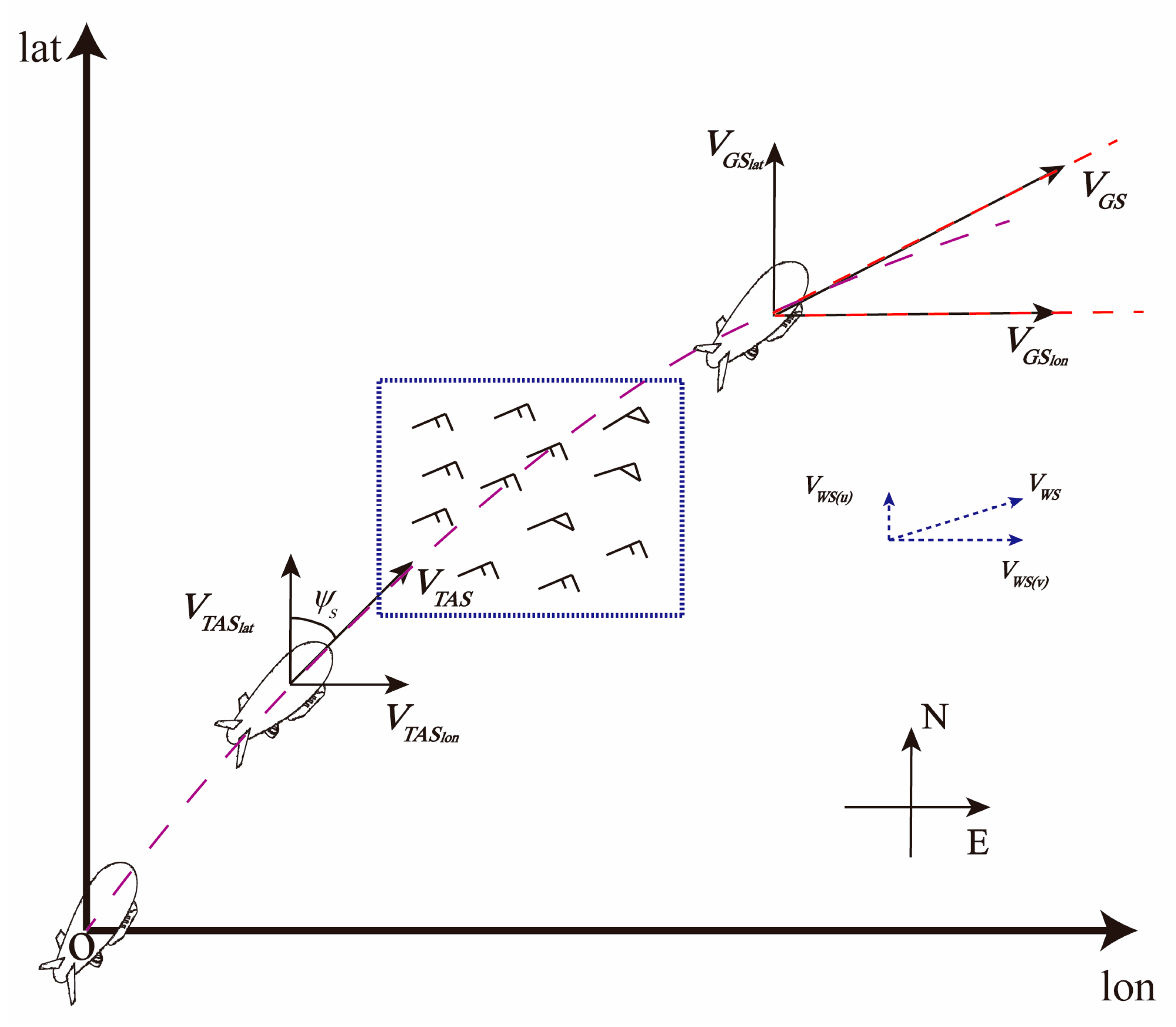
The kinematic model of the stratospheric airship developed in this study considers only speed and heading, and neglects sideslip. Under the influence of the wind field, the actual velocity of the airship—i.e., its ground speed V G S —is the vector sum of its true airspeed V T A S and the wind speed at its current state V W S , as shown in Equation (3), where x denotes the displacement.
V G S = V T A S + V W S V G S l o n V G S l a t = V T A S l o n + V W S ( v ) V T A S l a t + V W S ( u ) x ˙ = V G S
The airship’s true airspeed direction is aligned with its heading, which is defined as the angle ψ s between the true airspeed vector and the true north axis, as illustrated in Figure 2. The purple dashed line represents the mission path planned for the airship.

2.3.2. Energy Model

The energy model of the stratospheric airship mainly consists of three components: energy harvesting, consumption, and storage. Energy harvesting relies on a photovoltaic solar panel array mounted on the upper surface of the airship, which captures direct solar irradiance during daytime to support flight. This constitutes the primary energy source for the airship, as described in Equation (4).
W c e l l = η s × q s × S s
Here, W c e l l denotes the power generated by the solar cells, η s represents the photovoltaic conversion efficiency, and S s is the solar cell area.
q s = 0 t f l y I D × sin θ h d t
In the equation, I D denotes the solar direct irradiance per unit area per unit time. This value depends on the specific days selected throughout the year. In this study, the maximum duration of 20 days is chosen for experiments, and I D is calculated based on the formula provided by [44]. θ h represents the solar elevation angle, t denotes the time, and t f l y denotes the total flight duration.
Solar radiation collection mainly depends on the solar elevation angle, which is related to the airship’s current position and time, as expressed in Equation (6).
sin θ h = sin l a t × sin δ + cos l a t × cos δ × cos Ω
In the equations, δ and Ω denote the solar declination angle and hourly angle, respectively, with their calculation formulas given in Equations (7) and (8). Here, N is the number of experimental days selected within the year, N 0 is the total number of days in a year, and k 1 e n e r g y is a coefficient referenced from [31].
δ = k 1 e n e r g y cos 2 π N + 10 N 0
Ω = π 12 × t 12
The airship’s energy consumption primarily consists of three parts: the energy consumed by the propulsion system to drive the airship’s movement W d t , the energy used by the payload during the flight mission W p l , and the energy consumed by measurement, control, and avionics systems W c o n t r o l , as expressed in Equation (9).
W t o t a l = W d t + W p l + W c o n t r o l
This study considers the practical scenario where the energy consumed by the payload and the control system during the mission is constant within each time step. Based on this assumption, the above formula is simplified as follows:
W t o t a l = W d t + W p l + W c o n t r o l = P d t + P K × t
In the equation, P d t represents the power consumed by the propulsion system, and P K denotes the combined power of the payload and control systems within a single minimum time step. The propulsion system consists of motors driving propellers, and its power consumption can be expressed by the following combined formula:
P d t = F × V T A S η p r o t × η m o t F = 1 2 ρ a i r × S r e f × C D × V T A S 2
In the equation, η p r o t denotes the propeller efficiency, the motor efficiency η m o t , and the thrust generated by the propulsion system. ρ a i r represents the atmospheric density at the operating altitude, the reference area of the airship S r e f . In this study, the airship’s propulsion is provided by two motors controlling the east–west and north–south velocities separately.
The energy storage model is primarily used to store surplus energy in a battery when the power generated by the solar panel array exceeds the energy consumption. This stored energy can then be used to supplement power during periods of insufficient generation, as shown in Equation (12). W l i denotes the remaining energy in the battery, and W 0 represents the rated capacity of the battery. Based on practical engineering considerations, W 0 is set to 400 kWh in this study.
W l i = W c e l l W t o t a l     i f   W l i < W 0
In addition, to comprehensively characterize the energy status of the airship’s storage battery, the state of charge ( S O C ) is introduced as a key parameter. The S O C represents the battery’s charge level and is defined as the ratio of the remaining energy W l i to the rated capacity of the battery W 0 .
S O C = W l i W 0 × 100 %

2.4. MDP Model

2.4.1. Markov Decision Process

An agent selects an action a F t to execute based on the state s F t at the current time step t . After executing the action a F t , the state transitions from s F t to s F t + 1 and receives an environmental reward R F t + 1 . The process of the agent selecting actions is considered to have the Markov property, and this process is known as an MDP [45]. A Markov Decision Process is defined by a five-tuple M , which is
M = S F , A F , P a , R F , γ S F s F 1 , s F 2 , , s F t , A F a F 1 , a F 2 , , a F t , P a s F t , s F t + 1 = p s F t + 1 , R F t + 1 | s F t , R F t R F t + 1 = R F s F t , a F t
S F is the set of all possible states, where s F t S F represents the state at time step t ; A F is the set of all possible actions, where a F t A F represents the action executed at time step t ; P a s F t , s F t + 1 is the state transition probability in a complex and time-varying environment, representing the probability of transitioning from the current state s F t to a new state s F t + 1 after executing action a F t . Since the reinforcement learning algorithm used in this study falls under the category of model-free methods, the state transition process is modeled as deterministic, with the transition probability equal to 1. R F is the immediate reward function, R F t + 1 is the reward obtained after executing action a F t in state s F t . γ is the discount factor, with a range of 0 , 1 . The larger the γ , the greater the emphasis the agent places on future rewards. The following sections provide detailed descriptions of the state space, action space, and reward function design.

2.4.2. States and Actions

The state space is a fusion of environmental perception and airship state features. Environmental perception primarily includes real-time position, the real-time wind speed of the time-sequential uncertainty wind field, and the goal location. Thus, the environmental perception state is defined as l a t , l o n , V W S u , V W S v , θ W D , l a t g o a l , l o n g o a l , where θ W D denotes the wind direction at the airship’s current location. The airship’s internal state features are derived from a mathematical model that captures the dynamic changes in the airship’s state under the combined effects of the wind field, energy cycle status, and action strategy. Specifically, the mapped parameters include the battery energy state S O C . The input state is therefore represented as shown in Equation (15).
s F = l a t , l o n , V W S u , V W S v , θ W D , l a t g o a l , l o n g o a l , S O C , t f l y
Considering that the control variable for the airship is true airspeed, the basic action is defined as a combination of true airspeed and heading angle. The airship’s true speed is adjusted by varying the motor’s rotational speed, while the heading angle is denoted by ψ s . These two elements together form the basic action. It is worth noting that the airship has an energy threshold. When its energy level drops below this threshold, it ceases movement and only maintains essential communications and system operations, as shown in Equation (16).
a F = V T A S , ψ s V T A S 0     i f   W l i W min   a n d   W c e l l W t o t a l V T A S V T A S max

2.4.3. Reward Function

In the field of reinforcement learning, the reward model serves as the criterion by which an agent evaluates the actions taken under a given state. Therefore, careful design of the reward function, denoted as R F , is essential. The reward model proposed in this study is a composite reward composed of five components: goal reward R g o a l ¯ , distance penalty R d i s ¯ , boundary penalty R o u t ¯ , time reward R t ¯ , and energy reward R e n e r g y ¯ . These components work together to influence the agent’s behavior and guide it toward the desired objective. Specifically, to ensure that the autonomous transfer task is completed within the designated area, both a boundary penalty and a sparse positive reward near the goal are necessary. In addition, to encourage the agent to move toward the goal, the Euclidean distance between the agent’s current position and the goal is introduced as a distance-based reward, as shown in Equation (17). To prevent the agent from remaining stationary, the distance to the goal is assigned a negative reward—i.e., the closer the agent gets to the goal, the smaller the penalty compared to remaining in place.
D i s s F t , · = l a t s F t l a t g o a l 2 + l o n s F t l o n g o a l 2
The time–energy composite reward model incorporates an energy reward, in which the remaining energy in the storage system at the end of the flight is integrated into the reward function as the energy-related reward R e n e r g y ¯ = S O C . Additionally, the flight must satisfy a minimum energy threshold constraint throughout the process, as described in Equation (16). This model jointly considers two key factors—energy and time—to strike a balance between them, thereby producing a path that better aligns with the comprehensive performance requirements of real-world applications. By adjusting k 4 , k 5 , i.e., the relative weighting between time and energy in the model, the reward function can be flexibly adapted to different task requirements and priorities. Accordingly, customized path planning schemes can be optimized based on the specific time and energy requirements of different missions.
R F = k 1 × R g o a l ¯ + k 2 × R d i s ¯ + k 3 × R o u t ¯ + k 4 × R t ¯ + k 5 × R e n e r g y ¯
Among these reward functions, R g o a l ¯ and R o u t ¯ are the main reward items, and their magnitude should be consistent. R d i s ¯ , R t ¯ , and R e n e r g y ¯ as auxiliary rewards also need to be controlled within the same order of magnitude. The value of the main reward item is approximately ten times that of the secondary reward item, which can be achieved by adjusting the weight of each reward item.
To systematically identify the suitable parameter configuration, a grid search was conducted over a predefined hyperparameter space. This process aimed to determine the combination of reward weights that enables the agent to balance the objectives of time and energy. The search space was defined with reasonable ranges and step sizes for each weight parameter, ensuring comprehensive coverage of potential configurations while keeping the computation tractable. Finally, the weight parameters k 1 , , k 5 were determined as 0.25, 0.06, 0.25, 0.34, and 0.10, respectively.

3. Method

In this chapter, we provide a detailed description of the TD3 algorithm combined with high-reward prioritized experience replay and LSTM (RPL-TD3), designed to address the path planning problem for a stratospheric airship. The algorithm is based on an LSTM network and incorporates a high-reward prioritized experience replay mechanism (HR-PER). This approach not only enhances performance by capturing historical state information via the LSTM but also accelerates the convergence of the TD3 algorithm through the HR-PER mechanism. Section 3.1 firstly introduces the baseline algorithms DDPG and TD3; Section 3.2 then addresses the common challenge of slow convergence in off-policy methods by proposing the innovative high-reward prioritized replay mechanism. The final section presents the overall algorithm framework of RPL-TD3.

3.1. Twin Delayed Deep Deterministic Policy Gradient

In recent years, with the rapid advancement of artificial intelligence technology, DRL algorithms have been widely applied across various fields. These methods can generally be categorized into on-policy and off-policy approaches based on whether the data used to update the policy is generated by the current policy. On-policy methods require the agent to update its policy using data generated by the current policy itself [46]. Representative algorithms include REINFORCE, A2C (Advantage Actor–Critic), and the widely used PPO. Compared to on-policy methods, off-policy approaches allow the agent to update its policy using data from a replay buffer containing past experiences, enabling training with samples collected by different policies (including historical ones), thereby improving sample efficiency. For example, Twin Delayed Deep Deterministic Policy Gradient (TD3) is an advanced off-policy deep reinforcement learning algorithm capable of handling continuous state and action spaces [47]. TD3 is an improvement upon the Deep Deterministic Policy Gradient (DDPG) algorithm, representing a deterministic deep reinforcement learning approach within the Actor–Critic framework. DDPG was developed by extending the discrete-action-space DQN to continuous action spaces through the introduction of an Actor network. Instead of selecting discrete actions, DDPG improves action quality by following the gradient of the Q-value provided by the Critic network, thus addressing continuous control problems [46,48]. However, similar to DQN, DDPG suffers from the issue of overestimation of Q-values. To address this overestimation, TD3 combines DDPG with Double DQN, employing two networks to represent different Q-values and using the minimum Q-value as the target for updates, thereby mitigating persistent overestimation, as shown in Equation (19). Furthermore, TD3 adds noise to the actions output by the Actor target network and delays the Actor network updates to enhance algorithm stability.
y r , s = r + γ min i = 1 , 2 Q θ i s , π ϕ s + ε ε a ~ c l i p N a 0 , σ a , n , n

3.2. Algorithm Improvements

3.2.1. LSTM Network Architecture

The LSTM network is a specialized architecture of recurrent neural networks (RNNs), primarily designed to address the problems of vanishing and exploding gradients encountered when training on long sequences. Since the airship path planning problem involves long-sequence decision-making, LSTM is well-suited for long-duration and long-distance navigation tasks.
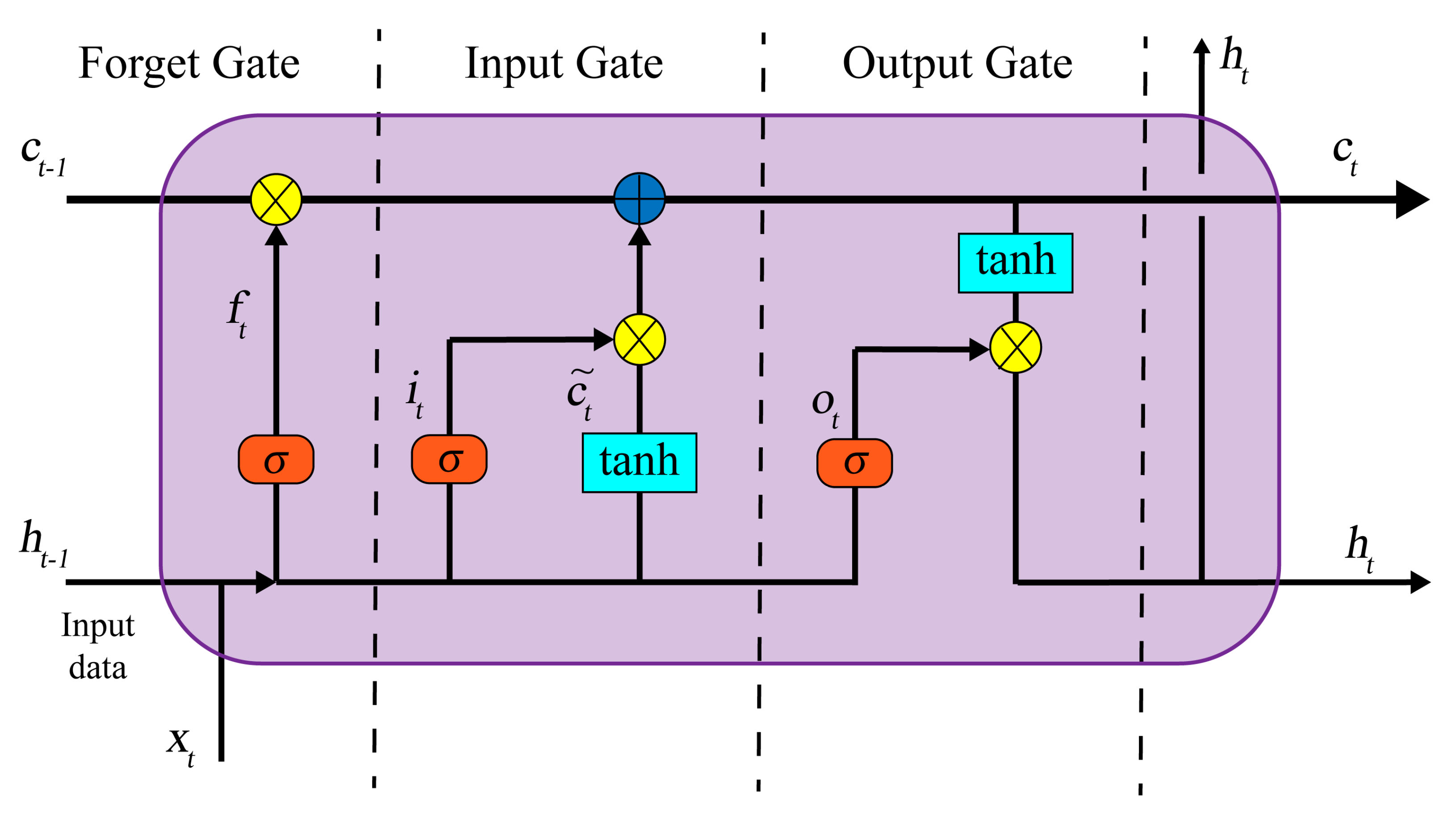
Conventional RNNs suffer from significant vanishing gradient issues when processing sequential data, especially for long sequences, where information from early time steps struggles to propagate effectively to later steps. This limitation arises from their simple recurrent structure. The core advantage of LSTM lies in its gating mechanisms, which effectively retain historical features, enabling superior performance on long sequences compared to conventional RNNs. The LSTM architecture consists of three gating mechanisms—input gate i t , forget gate f t , and output gate o t —and two state vectors: the cell state c t and the hidden state h t .
The network model, as shown in Figure 3, consists of three main computational processes: the forget process, the memory selection process, and the output process. Firstly, the neuron receives inputs, including the previous time step’s output h t 1 , the previous cell state c t 1 , and the current input x t . These inputs pass through the forget gate, which selectively removes information with smaller weights (discarded values f t ), followed by the input gate, which determines the information to be updated i t and the current cell state c ˜ t . Finally, in the output phase, the outputs of the forget gate and input gate combine to produce the long-term information and short-term information, which are stored and passed on to the next neuron. These processes can be represented by the following equations:
f t = σ W f × h t 1 , x t + b f i t = σ W i × h t 1 , x t + b i c ˜ t = tanh W c × h t 1 , x t + b c c t = f t × c t 1 + i t × c ˜ t o t = σ W o × h t 1 , x t + b o h t = o t × tanh c t

3.2.2. High-Reward Prioritized Experience Replay Mechanism (HR-PER)

The TD3 algorithm is a typical representative of off-policy methods. Like other off-policy algorithms, it suffers from challenges such as difficult and slow convergence, especially as the environment becomes more complex, where convergence becomes increasingly challenging. In this study, the stratospheric airship path planning task involves a multi-model coupled system navigating within a time-sequential environment, thus exhibiting high complexity. Therefore, this study proposes a high-reward prioritized experience replay mechanism, which is an improvement based on PER and EER. The mechanism will be explained from two perspectives: experience storage and retrieval, and priority assignment.
In traditional experience replay, experiences are stored and retrieved based on individual time-step samples—each interaction between the agent and the environment at a given moment, represented as a tuple of state, action, reward, and next state s F t , a F , R F , s F t + 1 , is stored as an independent experience i in the replay buffer. During training, traditional experience replay randomly samples experiences from the replay buffer to update model parameters. Although random sampling breaks temporal correlations between data, which may aid training stability, it disrupts the temporal structure inherent in the sequence. Since the stratospheric wind field environment is highly dynamic and time-sequential, and the airship path planning task involves long-term decision-making, the dependencies between consecutive time-step states are crucial for representing both the planning task and environmental dynamics. Therefore, purely random sampling from the replay buffer severs the temporal continuity, often hindering effective acceleration of convergence and making it difficult to learn reasonable policies early in training.
In RPL-TD3, inspired by EER, experience sampling is optimized to significantly accelerate convergence. This sampling approach stores each episode of agent–environment interactions as a sequential data chain in the replay buffer. During sampling, a random starting point in the chain is selected to extract a segment of length L i for training. This method preserves the broad sample utilization of random sampling while maintaining the temporal continuity of the experience chain, thus addressing the temporal disruption problem in traditional experience replay.
Moreover, to enhance the efficiency of utilizing valuable data during training, we draw on the concept of PER, where the importance of each experience is labeled to ensure that high-value experiences are sampled more frequently. The mainstream methods for assigning experience priority include proportional priority sampling and rank-based priority sampling. Both methods have shown comparable performance in experiments. However, since the reward values of experience sequences R i in this study vary significantly, rank-based priority sampling is adopted. Experiences are ranked by their reward values, and the sampling probability of each experience p i is assigned based on Equation (21).
p i = 1 r a n k i
In this study, the priority of sampled experiences is evaluated based on the total reward of the sequence. Accordingly, the sampling probability is no longer uniform, but instead follows a non-uniform distribution determined by the sampling criterion, as shown in Equation (22).
p i = p i 1 α k p k 1 α
If the learning process greedily focuses on repeatedly sampling only the highest-value experiences—i.e., the neural network is consistently updated using a fixed “subset of experiences”—it may easily lead to local optima or overestimation issues. To address this problem, a scaling factor 1 α is introduced, which follows a decay strategy. As training progresses, the scaling factor 1 α gradually decreases with the number of episodes n e p , controlled by a decay coefficient β . This allows the priority of high-value experiences to gradually increase, thereby accelerating model convergence. To ensure training stability, 1 α delayed parameter updates are employed, meaning the update is performed only once every c e p episode. The decay follows an exponential form, as shown in Equation (23):
1 α n e p + 1 = 1 α n e p × exp β × n e p     i f   n e p % c e p = 0
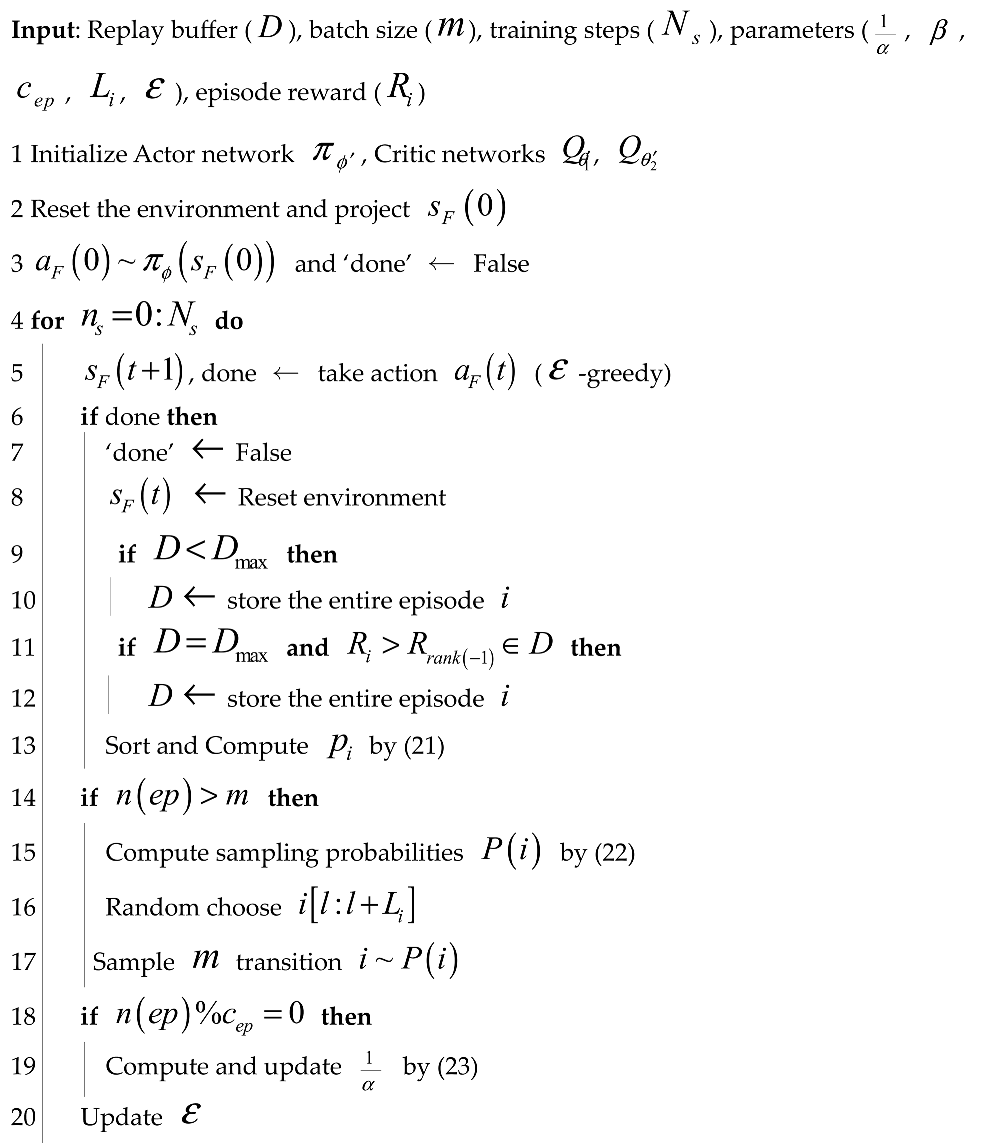
The detailed algorithmic procedure of the high-reward prioritized experience replay mechanism is presented in Algorithm 1.
Algorithm 1: HR-PER Algorithm
Drones 09 00650 i001

3.3. RPL-TD3 Algorithm Procedure

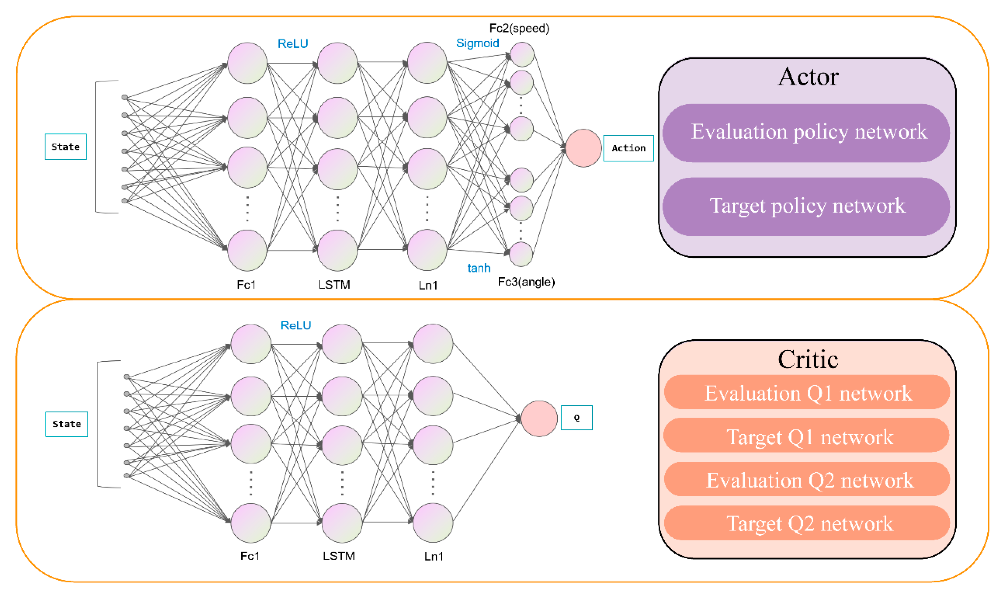
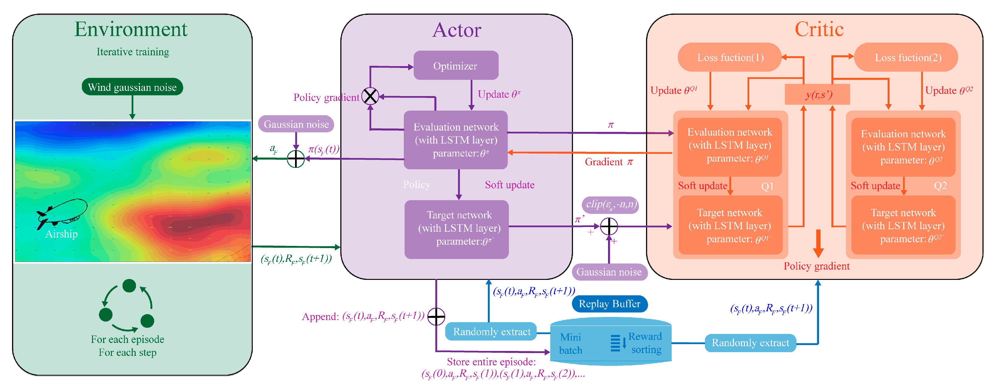
The RPL-TD3 algorithm extends the original TD3 framework by incorporating an LSTM network and a high-reward prioritized experience replay mechanism. The network architecture of RPL-TD3 is illustrated in Figure 4. The architecture consists of fully connected layers, an LSTM hidden layer, layer normalization, and an output layer. Notably, the Actor network contains two separate fully connected output layers—one outputs the desired velocity of the airship, and the other outputs the desired heading angle. The Sigmoid and Tanh functions are used as activation functions for these layers, respectively. The outputs are then combined to form the final desired action of the airship.
The airship then executes the desired action within the simulation environment. The environment calculates the next state and the corresponding immediate reward based on the current state and the received action. The RPL-TD3 algorithm collects this interaction data to form experience samples, which are stored and sampled using the high-reward prioritized replay mechanism. The Actor and Critic networks use the sampled experiences and the temporal features extracted by the LSTM to perform policy evaluation and improvement. This process continuously enhances the decision-making capability of the airship. Figure 5 illustrates the dynamic interaction between the RPL-TD3 algorithm and the simulation environment.

4. Experiments

In this chapter, the proposed RPL-TD3 algorithm is employed to train the stratospheric airship agent model within a simulation environment, aiming to accomplish path planning tasks under time-sequential uncertainty wind field conditions. Comparative experiments are conducted with other baseline algorithms, such as DDPG and TD3, to evaluate the performance of the proposed algorithm in autonomous transfer tasks. Finally, Section 4.3 presents the simulation results for the path planning task and the generalization experiments across multiple scenarios.

4.1. Experiment Setup

The experimental platform is configured with an Intel Xeon Silver 4214R CPU, an NVIDIA Tesla A40 GPU, and runs on the Ubuntu 20.04 operating system. The simulation environment is developed in Python 3.10, built upon the standard OpenAI Gym 0.25.2 framework, while all algorithmic implementations are based on PyTorch 2.5.1.
The simulation environment is constructed using ERA5 wind field data from January of a certain year, based on the time-sequential uncertainty wind field model described in Section 2.2. The stratospheric airship agent model follows the specification outlined in Section 2.3. Detailed simulation parameters are provided in Table 2.

4.2. Training of the Stratospheric Airship Path Planning Model

The simulation environment in this study considers only the influence of the wind field on the motion of the airship. At the beginning of training, two random locations within the regional wind field are selected as the starting and goal positions for the airship. A training episode terminates when the stratospheric airship moves out of bounds, its energy consumption falls below the minimum threshold, it reaches the vicinity of the goal point, or the maximum number of steps is exceeded. To ensure the fairness of the comparative experiments and the reliability of the conclusions, all algorithms in this study were implemented using widely validated standard network architectures and parameter settings. Specifically, the Actor and Critic networks of the baseline DDPG and TD3 algorithms employed fully connected layers with 128 neurons, optimized with Adam, with a replay buffer size of 3 × 10⁶ and a batch size of 128. For L-DDPG and L-TD3, the only modification was the replacement of the fully connected hidden layers with LSTM layers, while all other hyperparameters remained unchanged. The proposed RPL-TD3 algorithm was further built upon L-TD3 by introducing the HR-PER mechanism, with detailed parameter configurations summarized in Table 3.
During the early stages of training, the airship lacks a clear understanding of the primary task, which results in inefficient movement toward the goal due to the absence of a reasonable velocity strategy. As training progresses and historical decision data accumulates in the experience replay buffer, the airship agent gradually learns to focus on reaching the goal point. Due to the sparse reward setting, the agent initially fails to learn from distance-based, time-based, and energy-related rewards during flight, resulting in a relatively low average reward. After extensive training, the agent gradually learns to recognize auxiliary rewards, navigate more directly toward the goal, and refine its energy management strategies during flight to maintain a consistently high battery state of charge. The gradual increase in maximum reward values indicates that the model is converging.
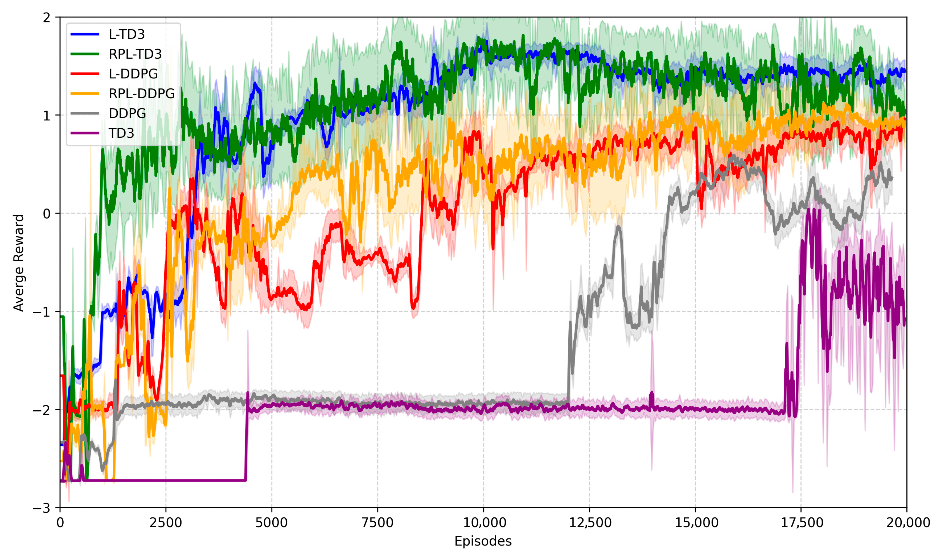
To evaluate the convergence performance of the proposed improved algorithm, comparative experiments were conducted among different algorithms, as illustrated in Figure 6. The blue, green, and purple curves correspond to the L-TD3 algorithm (TD3 with an LSTM layer), the proposed RPL-TD3 algorithm, and the baseline TD3 algorithm, respectively. The red, orange, and gray curves represent the L-DDPG algorithm (DDPG with an LSTM layer), the RPL-DDPG algorithm (DDPG with both high-reward prioritized replay and LSTM), and the baseline DDPG algorithm, respectively.
After 20,000 training iterations, the baseline algorithms TD3 and DDPG exhibited poor convergence performance, struggling to learn stable and high-reward planning policies. In contrast, the L-TD3 and L-DDPG algorithms, which incorporate LSTM layers, demonstrated significantly improved convergence characteristics, achieving higher average rewards upon convergence compared to the baseline methods. This improvement is primarily attributed to the fact that the baseline algorithms rely solely on fully connected layers to capture instantaneous state information, lacking memory capabilities. Given that the task involves strong temporal dependencies, LSTM networks—with their unique gated architecture comprising input, forget, and output gates, and recursive propagation of hidden and cell states—effectively model complex dependencies across historical time sequences, thereby significantly enhancing the algorithm’s performance.
As shown in the figure, L-TD3 requires approximately 4000 episodes to converge, whereas L-DDPG exhibits significant fluctuations in average reward throughout the training period. This indicates that simply incorporating LSTM layers does not effectively address the slow and difficult convergence issues commonly associated with off-policy algorithms. In contrast, RPL-TD3 and RPL-DDPG integrate a high-reward prioritized experience replay mechanism, which markedly improves both convergence performance and speed, as clearly evidenced by the figure. Specifically, compared to L-DDPG, RPL-DDPG nearly converges after 5000 episodes with reduced fluctuations in average reward, demonstrating enhanced convergence stability. Compared with L-TD3, RPL-TD3 converges after only 1500 episodes, representing a 62.5% increase in convergence speed. In summary, the proposed high-reward prioritized experience replay mechanism effectively accelerates convergence speed and improves convergence quality. In addition, although both RPL-TD3 and RPL-DDPG incorporate HR-PER, their final convergence performance and stability still exhibit significant differences. RPL-TD3 converges much faster than RPL-DDPG and achieves a higher average reward after convergence. The fundamental reason for this difference lies in the underlying base algorithms. As an improved version of DDPG, TD3 introduces three key mechanisms—Double Q-learning, Target Policy Smoothing, and Delayed Policy Update—which effectively alleviate the overestimation issue of Q-values commonly observed in DDPG. Consequently, even when integrated with the same LSTM and HR-PER modules, RPL-TD3, built on the more stable and robust TD3 foundation, naturally outperforms its DDPG-based counterpart. This comparison further validates that the proposed HR-PER mechanism serves as an effective “performance booster,” while its ultimate effectiveness remains constrained by the performance ceiling of the base algorithm on which it is applied.

4.3. Simulation Results of RPL-TD3

4.3.1. Comparative Simulation Experiments of RPL-TD3

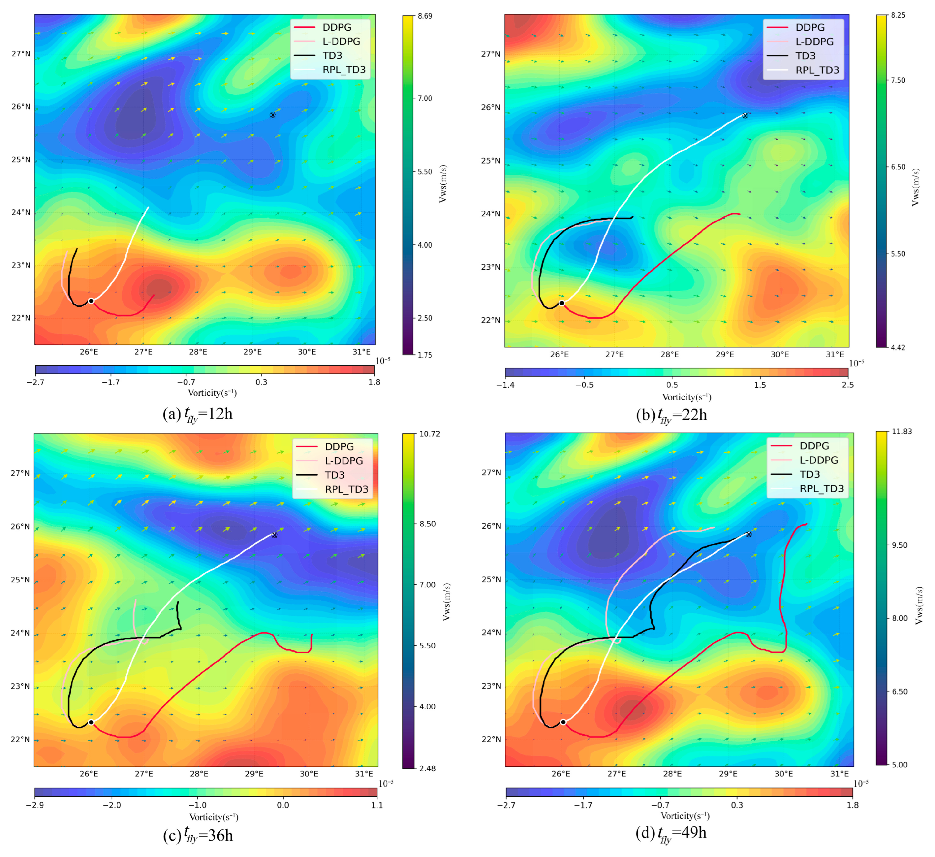
In Section 4.2, we trained path planning models using various algorithms. In this section, we conduct task testing within a designated area, including comparative experiments and generalization validation, to analyze and compare their performance in path planning tasks. Figure 7 shows the comparative results of four algorithms on a specific path planning task. The red, pink, black, and white lines represent the results of DDPG, L-DDPG, TD3, and RPL-TD3, respectively. The task is to plan a route from the start point (26.03° E, 22.35° N) to the goal point (28.12° E, 22.22° N) to complete an autonomous transfer mission. Figure 7 presents the planning results at four different time intervals, i.e., different time steps. At t f l y = 22   h , the path planned by the RPL-TD3 algorithm remained entirely within favorable tailwind regions, enabling the airship to utilize advantageous wind conditions and complete the planning task first, while the other algorithms failed to finish. At t f l y = 49   h , the TD3 algorithm also completed the planning task. The other two algorithms eventually reached the goal at t f l y = 55   h , 68   h , respectively. Comparing the four algorithms, we find that the path planned by RPL-TD3 is smoother and requires the shortest planning time.
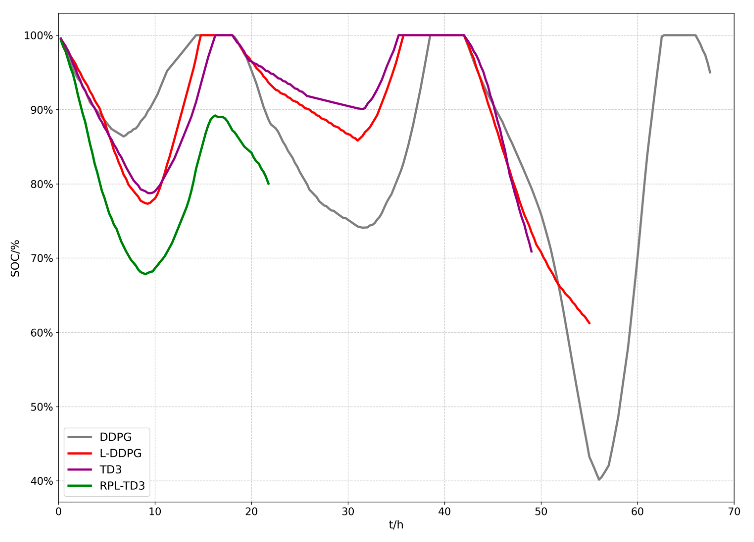
Figure 8 illustrates the S O C variation in the airship’s battery during the mission. It can be seen that at the start of the flight, since it is early morning with low solar irradiance, the airship’s power supply mainly relies on the stored battery energy, causing the S O C to gradually decrease from 100%. As the flight progresses, solar irradiance increases, and once the absorbed energy exceeds the airship’s current consumption, the battery begins to recharge, resulting in a rise in S O C .
The S O C curves of the energy storage batteries for the four algorithms correspond to the path planning results shown in Figure 8, with specific parameters detailed in Table 4. From the S O C variations, it can be observed that all four algorithms successfully completed the tasks within the minimum energy constraints, with average energy levels remaining above 80% throughout the missions. Among the evaluated methods, the TD3 algorithm achieved the highest energy efficiency, with an average residual energy of 96.51% and a minimum of 86.51%. The RPL-TD3 algorithm recorded an average residual energy of 89.63% and a minimum of 67.83%. Compared with the traditional TD3 algorithm, the proposed TD3-based approach exhibits only a slight difference in energy consumption, but reduces the task completion time by 27.25 h. This improvement is attributed to the lower path redundancy and the effective exploitation of favorable wind conditions enabled by the RPL-TD3 algorithm. In summary, the RPL-TD3 algorithm demonstrates superior performance in path planning tasks under both time and energy constraints, outperforming other comparable methods.

4.3.2. Generalization Experiments

To verify the model’s reliability, this study designed multi-scenario generalization experiments by randomly selecting start and end points within a designated area to construct diverse task scenarios, simulating real-world path planning tasks. The testing process was conducted 500 times within the same time-sequential uncertainty wind field. Results show that the RPL-TD3 algorithm achieved a path planning success rate of 93.3%. It is noteworthy that the unsuccessful cases were primarily attributed to extreme wind conditions (such as persistent headwinds or drastic wind direction changes), where the airship’s propulsion was insufficient to overcome the wind disturbances within the limited time frame.
The final navigation outcomes are shown in Figure 9, with only partial scenario results presented. The specific test parameters corresponding to these scenarios, such as flight time, are shown in Table 5. The upper right corner of each subplot annotates the latitude and longitude coordinates of the start and goal positions. The red curve represents the path planned by the algorithm, the black dot indicates the start position, and the cross marks the goal position. When the airship enters the threshold area around the goal point (shown as the dashed circle in the figure), it is considered to have reached the goal. In Figure 9, the airship successfully reaches the goal point in various task scenarios. The airship’s model constraints, goal location, and wind field model all influence the choice of the optimal policy, i.e., the optimal action sequence, which results in variations in the planned paths. Overall, the RPL-TD3 algorithm can successfully plan relatively smooth paths. It has learned an efficient and stable planning strategy that significantly reduces path redundancy while satisfying model constraints.
The final navigation outcomes are shown in Figure 9, with only partial scenario results presented. The specific test parameters corresponding to these scenarios, such as flight time, are shown in Table 5. The upper right corner of each subplot annotates the latitude and longitude coordinates of the start and goal positions. The red curve represents the path planned by the algorithm, the black dot indicates the start position, and the cross marks the goal position. When the airship enters the threshold area around the goal point (shown as the dashed circle in the figure), it is considered to have reached the goal. In Figure 9, the airship successfully reaches the target point in various task scenarios. The airship’s model constraints, goal location, and wind field model all influence the choice of the optimal policy, i.e., the optimal action sequence, which results in variations in the planned paths. Overall, the RPL-TD3 algorithm can successfully plan relatively smooth paths. It has learned an efficient and stable planning strategy that significantly reduces path redundancy while satisfying model constraints.
To further evaluate the generalization capability and robustness of the model under different environments, small-sample tests were conducted using wind field data from March and May of a certain year. In March, the average wind speed was 12.31 m/s with a maximum of 23.34 m/s, while in May, the average wind speed was 6.72 m/s with a maximum of 20.56 m/s. The results indicate that the path planning success rates of the proposed RPL-TD3 algorithm were 73.33% and 86.67%, respectively. This result demonstrates the algorithm’s adaptability and stability under different wind field conditions. In particular, it remained effective in path planning during the extreme meteorological conditions of March, showcasing strong potential for practical applications.

5. Discussion and Conclusions

This study focuses on the path planning task of a stratospheric airship under a time-sequential uncertainty wind field. By introducing innovative mechanisms such as LSTM networks and reward-prioritized experience replay, the performance of deep reinforcement learning algorithms in terms of convergence and policy capability is improved. Through simulations and comparative experiments, we demonstrate the effectiveness of the proposed method in autonomous transfer tasks of a stratospheric airship.
  • Based on the mathematical model of stratospheric airship path planning, this study uses the airship’s state and environmental information as observation data, with true airspeed and heading angle combined as action outputs. A time–energy composite reward model is designed to guide the agent’s learning. By interacting with the environment to train the deep neural network, a suitable and stable planning policy eventually converged.
  • The proposed RPL-TD3 algorithm enhances planning capability by integrating an LSTM network, aiming to improve performance in strongly time-dependent path planning tasks. Additionally, to address the slow and difficult convergence of off-policy algorithms, a reward-prioritized experience replay mechanism is introduced, prioritizing high-value experiences to accelerate convergence. Comparative experiments show that RPL-TD3 exhibits strong convergence, with a 62.5% improvement in convergence speed compared to versions without reward-prioritized replay.
  • Simulation results demonstrate that the proposed method is capable of generating feasible paths under kinematic and energy constraints. Compared with other baseline algorithms, it achieves the shortest flight time while maintaining a relatively high level of average residual energy. Furthermore, in multi-scenario generalization experiments, the RPL-TD3 algorithm attained a 93.3% success rate and significantly reduced path redundancy while satisfying model constraints.
However, this study only considers the impact of wind fields on the airship path planning task, and the generalization experiments are validated using wind field data from a single month. In practical applications, various environmental factors, such as high-altitude cold clouds, can significantly affect flight missions. In addition, seasonal variations also influence stratospheric wind fields. Future research will focus on incorporating more realistic flight environment models and introducing cross-seasonal and multi-year wind field data for training and testing, in order to enhance the robustness of path planning algorithms under complex conditions and to further advance the application of artificial intelligence in this field.

Author Contributions

Methodology, J.X.; Investigation, S.C.; Writing—original draft, J.X.; Writing—review & editing, J.M.; Visualization, J.L.; Supervision, W.H.; Funding acquisition, W.H. All authors have read and agreed to the published version of the manuscript.

Funding

This research was funded by the National Key R&D Program of China, grant number 2022YFB3207300.

Data Availability Statement

The original contributions presented in the study are included in the article, further inquiries can be directed to the corresponding author.

Conflicts of Interest

The authors declare no conflicts of interest.

References

  1. Belmont, A.D.; Dartt, D.G.; Nastrom, G.D. Variations of stratospheric zonal winds, 20–65 km, 1961–1971. J. Appl. Meteorol. Climatol. 2010, 14, 585–594. [Google Scholar] [CrossRef]
  2. Hong, Y.J. Aircraft Technology of Near Space; National University of Defense Technology Press: Beijing, China, 2012; pp. 9–12. [Google Scholar]
  3. Schaefer, I.; Kueke, R.; Lindstrand, P. Airships as unmanned platforms: Challenge and chance. In Proceedings of the 1st UAV Conference, Portsmouth, VA, USA, 20–23 May 2002; p. 3423. [Google Scholar]
  4. d’Oliveira, F.A.; Melo, F.C.L.D.; Devezas, T.C. High-altitude platforms—Present situation technology trends. J. Aerosp. Technol. Manag. 2016, 8, 249–262. [Google Scholar] [CrossRef]
  5. Manikandan, M.; Pant, R.S. Research and advancements in hybrid airships—A review. Prog. Aerosp. Sci. 2021, 127, 100741. [Google Scholar] [CrossRef]
  6. Shaw, J.A.; Nugent, P.W.; Kaufman, N.A.; Pust, N.J.; Mikes, D.; Knierim, C.; Faulconer, N.; Larimer, R.M.; DesJardins, A.C.; Knighton, W.B. Multispectral imaging systems on tethered balloons for optical remote sensing education and research. J. Appl. Remote Sens. 2012, 6, 063613. [Google Scholar] [CrossRef]
  7. Golkar, A. Experiential systems engineering education concept using stratospheric balloon missions. IEEE Syst. J. 2019, 14, 1558–1567. [Google Scholar] [CrossRef]
  8. Jones, W.V. Evolution of scientific ballooning and its impact on astrophysics research. Adv. Space Res. 2014, 53, 1405–1414. [Google Scholar] [CrossRef]
  9. Azinheira, J.; Carvalho, R.; Paiva, E.; Cordeiro, R. Hexa-Propeller Airship for Environmental Surveillance and Monitoring in Amazon Rainforest. Aerospace 2024, 11, 249. [Google Scholar] [CrossRef]
  10. S. INC. Sceye Airships. 2021. Available online: https://www.sceye.com/ (accessed on 10 March 2025).
  11. Alam, M.I.; Pasha, A.A.; Jameel, A.G.A.; Ahmed, U. High Altitude Airship: A Review of Thermal Analyses and Design Approaches. Arch. Comput. Methods Eng. 2023, 30, 2289–2339. [Google Scholar] [CrossRef]
  12. Chen, P.; Huang, Y.; Papadimitriou, E.; Mou, J.; van Gelder, P. Global path planning for autonomous ship: A hybrid approach of fast marching square and velocity obstacles methods. Ocean Eng. 2020, 214, 107793. [Google Scholar] [CrossRef]
  13. Sands, T. Virtual sensoring of motion using Pontryagin’s treatment of Hamiltonian systems. Sensors 2021, 21, 4603. [Google Scholar] [CrossRef] [PubMed]
  14. Vashisth, A.; Rückin, J.; Magistri, F.; Stachniss, C.; Popović, M. Deep reinforcement learning with dynamic graphs for adaptive informative path planning. IEEE Robot. Autom. Lett. 2024, 9, 7747–7754. [Google Scholar] [CrossRef]
  15. Yang, Y.; Fu, Y.; Xin, R.; Feng, W.; Xu, K. Multi-UAV Trajectory Planning Based on a Two-Layer Algorithm Under Four-Dimensional Constraints. Drones 2025, 9, 471. [Google Scholar] [CrossRef]
  16. MTipaldi, R.; Iervolino, P.R. Massenio, Reinforcement learning in spacecraft control applications: Advances, prospects, and challenges. Annu. Rev. Control 2022, 54, 1–23. [Google Scholar] [CrossRef]
  17. Xie, G.; Fang, L.; Su, X.; Guo, D.; Qi, Z.; Li, Y.; Che, J. Research on Risk Avoidance Path Planning for Unmanned Vehicle Based on Genetic Algorithm and Bezier Curve. Drones 2025, 9, 126. [Google Scholar] [CrossRef]
  18. Cândido, B.; Rodrigues, C.; Moutinho, A.; Azinheira, J.R. Modeling, Altitude Control, and Trajectory Planning of a Weather Balloon Subject to Wind Disturbances. Aerospace 2025, 12, 392. [Google Scholar] [CrossRef]
  19. Luo, Q.; Sun, K.; Chen, T.; Zhang, Y.-F.; Zheng, Z.-W. Trajectory planning of stratospheric airship for station-keeping mission based on improved rapidly exploring random tree. Adv. Space Res. 2024, 73, 992–1005. [Google Scholar] [CrossRef]
  20. Hu, Z.D.; Xia, Q.; Cai, H. Various Stochastic Search Algorithms for High-Altitude Airship Trajectory Planning. Comput. Simul. 2007, 7, 55–58. [Google Scholar]
  21. Sun, H.; Zhang, W.; Yu, R.; Zhang, Y. Motion planning for mobile robots—Focusing on deep reinforcement learning: A systematic review. IEEE Access 2021, 9, 69061–69081. [Google Scholar] [CrossRef]
  22. Zhao, X.; Yang, R.; Zhong, L.; Hou, Z. Multi-UAV Path Planning and Following Based on Multi-Agent Reinforcement Learning. Drones 2024, 8, 18. [Google Scholar] [CrossRef]
  23. Panov, A.I.; Yakovlev, K.S.; Suvorov, R. Grid path planning with deep reinforcement learning: Preliminary results. Procedia Comput. Sci. 2018, 123, 347–353. [Google Scholar] [CrossRef]
  24. Bellemare, M.G.; Candido, S.; Castro, P.S.; Gong, J.; Machado, M.C.; Moitra, S.; Ponda, S.S.; Wang, Z. Autonomous navigation of stratospheric balloons using reinforcement learning. Nature 2020, 588, 77–82. [Google Scholar] [CrossRef]
  25. Xu, Z.; Liu, Y.; Du, H.; Lv, M. Station-keeping for high-altitude balloon with reinforcement learning. Adv. Space Res. 2022, 70, 733–751. [Google Scholar] [CrossRef]
  26. Bai, F.; Yang, X.; Deng, X.; Ma, Z.; Long, Y. Station keeping control method based on deep reinforcement learning for stratospheric aerostat in dynamic wind field. Adv. Space Res. 2024, 75, 752–766. [Google Scholar] [CrossRef]
  27. Luo, Q.; Sun, K.; Chen, T.; Zhu, M.; Zheng, Z. Stratospheric airship fixed-time trajectory planning based on reinforcement learning. Electron. Res. Arch. 2025, 33, 1946–1967. [Google Scholar] [CrossRef]
  28. Zheng, B.; Zhu, M.; Guo, X.; Ou, J.; Yuan, J. Path planning of stratospheric airship in dynamic wind field based on deep reinforcement learning. Aerosp. Sci. Technol. 2024, 150, 109173. [Google Scholar] [CrossRef]
  29. Liu, S.; Zhou, S.; Miao, J.; Shang, H.; Cui, Y.; Lu, Y. Autonomous Trajectory Planning Method for Stratospheric Airship Regional Station-Keeping Based on Deep Reinforcement Learning. Aerospace 2024, 11, 753. [Google Scholar] [CrossRef]
  30. Hausknecht, M.; Stone, P.; Mc, O. On-policy vs. off-policy updates for deep reinforcement learning. In Deep Reinforcement Learning: Frontiers and Challenges, IJCAI 2016 Workshop; AAAI Press: New York, NY, USA, 2016. [Google Scholar]
  31. Qi, L.; Yang, X.; Bai, F.; Deng, X.; Pan, Y. Stratospheric airship trajectory planning in wind field using deep reinforcement learning. Adv. Space Res. 2025, 75, 620–634. [Google Scholar] [CrossRef]
  32. Wang, Y.; Zheng, B.; Lou, W.; Sun, L.; Lv, C. Trajectory planning of stratosphere airship in wind-cloud environment based on soft actor-critic. In Proceedings of the 2024 IEEE International Conference on Artificial Intelligence in Engineering and Technology (IICAIET), Kota Kinabalu, Malaysia, 26–28 August 2024; pp. 401–406. [Google Scholar]
  33. Hou, J.; Zhu, M.; Zheng, B.; Guo, X.; Ou, J. Trajectory Planning Based On Continuous Decision Deep Reinforcement Learning for Stratospheric Airship. In Proceedings of the 2023 China Automation Congress (CAC), Chongqing, China, 17–19 November 2023; pp. 1508–1513. [Google Scholar]
  34. He, Y.; Guo, K.; Wang, C.; Fu, K.; Zheng, J. Path Planning for Autonomous Balloon Navigation with Reinforcement Learning. Electronics 2025, 14, 204. [Google Scholar] [CrossRef]
  35. Lv, C.; Zhu, M.; Guo, X.; Ou, J.; Lou, W. Hierarchical reinforcement learning method for long-horizon path planning of stratospheric airship. Aerosp. Sci. Technol. 2025, 160, 110075. [Google Scholar] [CrossRef]
  36. Neves, D.E.; Ishitani, L.; do Patrocinio Junior, Z.K.G. Advances and challenges in learning from experience replay. Artif. Intell. Rev. 2024, 58, 54. [Google Scholar] [CrossRef]
  37. Özalp, R.; Varol, N.K.; Taşci, B.; Uçar, A. A review of deep reinforcement learning algorithms and comparative results on inverted pendulum system. Mach. Learn. Paradig. Adv. Deep. Learn.-Based Technol. Appl. 2020, 18, 237–256. [Google Scholar]
  38. Hou, Y.; Liu, L.; Wei, Q.; Xu, X.; Chen, C. A novel DDPG method with prioritized experience replay. In Proceedings of the 2017 IEEE International Conference on Systems, Man, and Cybernetics (SMC), Banff, AB, Canada, 5–8 October 2017; pp. 316–321. [Google Scholar]
  39. Schaul, T.; Quan, J.; Antonoglou, I.; Silver, D. Prioritized experience replay. arXiv 2016, arXiv:1511.05952. [Google Scholar] [CrossRef]
  40. Hassani, H.; Nikan, S.; Shami, A. Traffic navigation via reinforcement learning with episodic-guided prioritized experience replay. Eng. Appl. Artif. Intell. 2024, 137, 109147. [Google Scholar] [CrossRef]
  41. Smierzchała, Ł.; Kozłowski, N.; Unold, O. Anticipatory Classifier System With Episode-Based Experience Replay. IEEE Access 2023, 11, 41190–41204. [Google Scholar] [CrossRef]
  42. Hersbach, H.; Bell, B.; Berrisford, P.; Biavati, G.; Horányi, A.; Muñoz Sabater, J.; Nicolas, J.; Peubey, C.; Radu, R.; Rozum, I.; et al. ERA5 Hourly Data on Single Levels from 1979 to Present. Copernic. Clim. Change Serv. (C3s) Clim. Data Store (Cds) 2018, 10. [Google Scholar]
  43. Wolf, M.T.; Blackmore, L.; Kuwata, Y.; Fathpour, N.; Elfes, A.; Newman, C. Probabilistic motion planning of balloons in strong, uncertain wind fields. In Proceedings of the 2010 IEEE International Conference on Robotics and Automation, Piscataway, NJ, USA, 3–7 May 2010; pp. 1123–1129. [Google Scholar]
  44. Li, J.; Liao, J.; Liao, Y.; Du, H.; Luo, S.; Zhu, W.; Lv, M. An approach for estimating perpetual endurance of the stratospheric solar-powered platform. Aerosp. Sci. Technol. 2018, 79, 118–130. [Google Scholar] [CrossRef]
  45. Shani, G.; Heckerman, D.; Brafman, R.I. An MDP-based recommender system. J. Mach. Learn. Res. 2005, 6, 1265–1295. [Google Scholar]
  46. Andrychowicz, M.; Raichuk, A.; Stańczyk, P.; Orsini, M.; Girgin, S.; Marinier, R.; Hussenot, L.; Geist, M.; Pietquin, O.; Michalski, M.; et al. What matters in on-policy reinforcement learning? a large-scale empirical study. arXiv 2020, arXiv:2006.05990. [Google Scholar]
  47. Fujimoto, S.; Hoof, H.; Meger, D. Addressing function approximation error in actor-critic methods. In Proceedings of the International Conference on Machine Learning, Stockholm, Sweden, 3 July 2018; pp. 1587–1596. [Google Scholar]
  48. Lillicrap, T.P.; Hunt, J.J.; Pritzel, A.; Heess, N.; Erez, T.; Tassa, Y.; Silver, D.; Wierstra, D. Continuous control with deep reinforcement learning. arXiv 2015, arXiv:1509.02971. [Google Scholar]
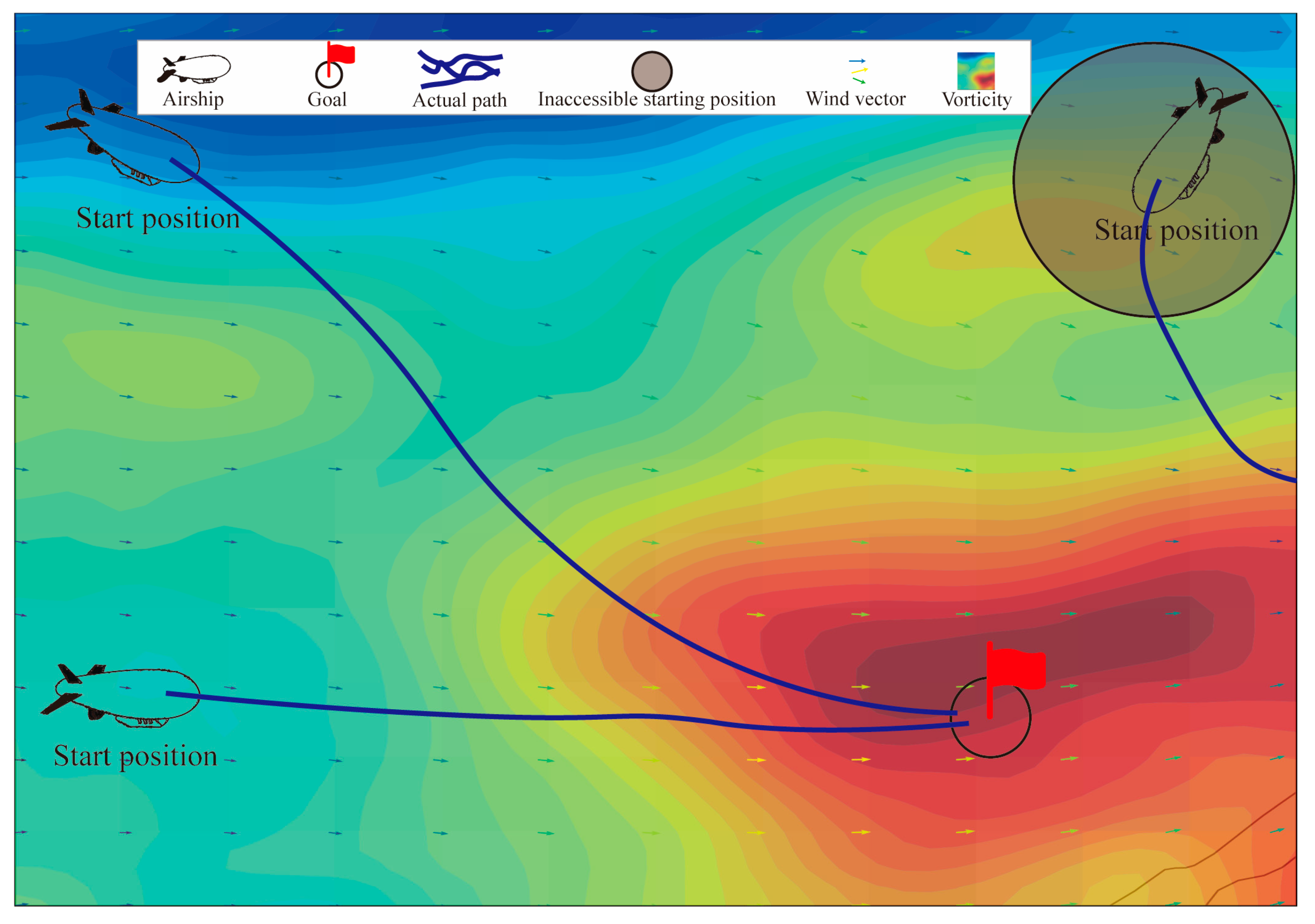
Figure 1. Illustration of the airship path planning task scenario.
Drones 09 00650 g001
Figure 2. Airship movement characteristics.
Drones 09 00650 g002
Figure 3. The LSTM network iterative calculation process.
Drones 09 00650 g003
Figure 4. The Actor and Critic network structure of the RPL-TD3 algorithm.
Drones 09 00650 g004
Figure 5. The RPL-TD3 algorithm and environment interaction process.
Drones 09 00650 g005
Figure 6. Comparison of training results for RPL-TD3, RPL-DDPG, L-TD3, L-DDPG, TD3, and DDPG (evaluation metric: average reward; higher values indicate better performance).
Drones 09 00650 g006
Figure 7. Path planning results of four algorithms (red, pink, black, and white represent DDPG, L-DDPG, TD3, and RPL-TD3, respectively).
Drones 09 00650 g007
Figure 8. Planning results of four algorithms: energy storage battery S O C curves.
Drones 09 00650 g008
Figure 9. Generalization validation results of RPL-TD3 algorithm.
Drones 09 00650 g009
Table 1. Summary of notations.
SymbolDescription
f G S V W S , V W S ¯ , σ W S Probability distribution function of meridional and zonal wind speed (average wind speed and standard deviation)
V W S a l l ¯ , ρ the average wind speed of all states in the local region and the Gaussian distribution coefficient
W S v , W S u , θ W D Meridional wind, zonal wind, and wind direction angle
V G S , V T A S , V W S , ψ s Airship ground speed, true airspeed, wind speed at its location, and heading angle
W c e l l , W l i , W 0 , W min Solar cells generate energy, the remaining energy of storage batteries, the rated capacity of batteries, and the minimum energy threshold for normal system operation
W t o t a l , W d t , W p l , W c o n t r o l The total energy consumption of the airship, propulsion system energy consumption, payload energy consumption, and measurement, avionics control system energy consumption
P d t , P K The total power of the airship propulsion system and the power consumption of other parts
η s , η p r o t , η m o t Solar cell photovoltaic conversion efficiency, airship propulsion system propeller efficiency, and motor efficiency
S s , S r e f The total area of solar cells on the stratospheric airship and the reference area of the stratospheric airship
q s , I D The power generation of solar cells per unit area and the direct solar irradiance per unit area per unit time
θ h , δ , Ω Solar elevation angle, solar declination angle, and hourly angle
ρ a i r , C D Atmospheric density and drag coefficient at the flight altitude of the stratospheric airship
N , N 0 The number of experimental days and the total number of days selected within one year
t f l y , S O C Total flight time and the state of charge for storage battery
s F t , a F t The agent’s state and action taken by the agent at time t
M S F , A F , P a , R F , γ MDP five-tuple (state space, action space, state transition probability, reward function, discount factor)
R g o a l ¯ , R d i s ¯ , R o u t ¯ , R t ¯ , R e n e r g y ¯ Agent rewards upon goal reward, distance penalty, boundary penalty, time reward, and energy reward
D i s s F t , · The distance function between the current position and the goal position of the stratospheric airship agent
k 1 , k 2 , k 3 , k 4 , k 5 Reward function R F weight parameters
y r , s , Q θ i , π ϕ Critic network target value, Critic network estimate value and Actor network policy
ε Exploration rate of the agent’s decision-making
θ π , θ Q Actor network parameters and Critic network parameters
ε a , N a 0 , σ a , n Target policy for smoothing noise, noise distribution, and clipping limit
i t , f t , o t The information of the input gate, forget gate and output gate of the LSTM neuron
c t , h t LSTM neuron cell state (combination of long- and short-term information) and hidden state (short-term memory)
x t , c ˜ t Current input and current state of LSTM neuron
σ , W f , b f Sigmoid layer (in LSTM), weight matrix, and bias vector
i , L i , R i , p i , P i Individual experience, experience sequence length, reward of individual experience, self-sampling probability of individual experience, and sampling probability
1 α , β Adaptive decay scaling factor and decay coefficient
n s , N s Current training step and total training steps
n e p , c e p Current episode and delayed update episode
Table 2. Simulation environment parameters.
ParametersValue
Wind field spatial resolution0.25°
Wind field time resolution1 h
Maximum true speed of airship15 m/s
Minimum energy of airship S O C 20%
Wing field size21.5° N–22.75° N, 25° E–31.25° E
Table 3. Experiment parameters.
ParametersValue
Batch size m 128
Hidden layer dimension128
Discount rate γ 0.99
Replay buffer D 3 × 10⁶
OptimizerAdam
Actor learning rate3 × 10−4
Critic learning rate3 × 10−4
Experience sequence length L i 1 × 10³
Delayed policy update frequency2
Target policy smoothing regularization1 × 10−2
Time-step interval15 min
Table 4. Path planning results of four algorithms.
AlgorithmDDPGL-DDPGTD3RPL-TD3
Flight time  t f l y 67.5 h55 h49 h21.75 h
Average energy  S O C 84.70%88.54%91.77%89.63%
Min energy  S O C 40.15%61.25%70.87%67.83%
Table 5. Generalization verification results of RPL-TD3 algorithm in different scenarios.
ScenarioStartGoalFlight Time t f l y Average Energy S O C
1(25.50° E, 23.55° N)(28.37° E, 26.85° N)21.25 h92.23%
2(28.99° E, 24.03° N)(26.98° E, 23.16° N)8.75 h69.78%
3(28.46° E, 25.56° N)(30.88° E, 25.30° N)28.25 h89.55%
4(31.11° E, 24.55° N)(29.33° E, 26.57° N)9.50 h76.34%
5(26.47° E, 22.30° N)(28.56° E, 25.62° N)18.00 h93.23%
6(26.02° E, 22.58° N)(30.23° E, 24.44° N)30.50 h85.78%
7(27.36° E, 24.85° N)(30.91° E, 23.10° N)22.50 h90.30%
8(26.12° E, 23.84° N)(29.67° E, 21.84° N)48.75 h80.26%
9(31.12° E, 25.86° N)(28.12° E, 22.22° N)33.00 h74.35%
10(29.04° E, 24.36° N)(30.25° E, 26.13° N)11.25 h78.85%
11(27.09° E, 25.84° N)(25.11° E, 25.85° N)4.50 h83.24%
12(25.54° E, 26.60° N)(30.85° E, 26.30° N)27.75 h90.18%
13(25.91° E, 25.56° N)(27.90° E, 27.12° N)12.75 h81.66%
14(26.19° E, 22.26° N)(29.59° E, 22.95° N)22.50 h88.49%
15(29.77° E, 24.49° N)(26.87° E, 24.75° N)7.00 h71.28%
16(29.85° E, 25.78° N)(30.72° E, 24.03° N)4.50 h80.49%
17(26.91° E, 25.93° N)(30.36° E, 26.29° N)13.50 h87.54%
18(26.47° E, 22.30° N)(28.56° E, 25.62° N)13.00 h84.88%
19(26.22° E, 22.91° N)(26.69° E, 27.01° N)24.50 h84.83%
20(26.00° E, 22.98° N)(30.02° E, 24.33° N)15.25 h76.45%
Disclaimer/Publisher’s Note: The statements, opinions and data contained in all publications are solely those of the individual author(s) and contributor(s) and not of MDPI and/or the editor(s). MDPI and/or the editor(s) disclaim responsibility for any injury to people or property resulting from any ideas, methods, instructions or products referred to in the content.