Error-Constrained Fixed-Time Synchronized Trajectory Tracking Control for Unmanned Airships with Disturbances

Abstract

This work focuses on fixed-time synchronized trajectory tracking control for unmanned airships subject to time-varying error constraints and unknown disturbances. First, to guarantee strict adherence to prescribed performance bounds, an error transformation function (ETF) is integrated into the control algorithm, which can ensure all tracking errors remain within specified constraints throughout the convergence process. Then, a Norm-Normalized sign (NNS) function is incorporated to develop the control scheme, guaranteeing simultaneous convergence of all tracking error components. Additionally, a novel fixed-time synchronized disturbance observer (FTSDO) is constructed and implemented to achieve precise disturbance estimation while ensuring synchronous convergence of the estimation errors. Finally, the developed control strategy is analytically verified to guarantee fixed-time synchronized stability (FTSS). To assess its performance, multiple simulations are executed. The results clearly demonstrate the proposed control scheme enables the airship to track the prescribed trajectory precisely in fixed time, and the convergence of all tracking error components is achieved synchronously.

1. Introduction

The development of unmanned systems has revolutionized their applications, such as enabling access to extreme operational environments inaccessible to manned systems, order-of-magnitude cost reductions in aerial operations, and extended-endurance missions [1]. As a distinctive kind of unmanned aerial vehicles, unmanned airships, possessing the ability to stay aloft for months, ideally, have attracted considerable interest owing to their promising commercial and military applications. In contrast to other passive aircraft requiring continuous human intervention, unmanned airships are capable of accurately tracking prescribed trajectories autonomously with validated control strategies. However, airships represent complex multivariable dynamical systems exhibiting inherent nonlinearities, strong inter-axis coupling, and susceptibility to multiple unknown disturbances arising from the stratosphere’s highly dynamic and uncertain operational environment. Consequently, advanced trajectory tracking control methods are required, rendering this field a crucial focus of continued research. Notably, various advanced methods including reinforcement learning [2,3] control, sliding mode control [4,5], model predictive control (MPC) [6,7], and backstepping control [8,9] have been applied to tackle these challenges. For example, Airaldi et al. [6] innovatively embedded a reinforcement learning method into the MPC framework. Starting from a model-inexact and suboptimally tuned MPC controller, this approach effectively learned to improve control policy. The authors in [10] established an innovative sliding mode controller for underactuated systems, employing a Newton–Euler formulation that achieved all-state stabilization of quadrotor vehicles despite model uncertainties and persistent disturbances.

Within the motion control of the unmanned vehicle, finite-time and fixed-time control have spurred a proliferation of related achievements. In theory, the stabilization time of finite-time controllers varies with initial conditions, leading to limited applications under scenario of unknown initial conditions [11]. Furthermore, fixed-time control has been developed and possesses a predefined convergent time independent of initial condition, ensuring preferable predictability [12,13]. In recent years, significant progress has been made in fixed-time control of unmanned vehicles. Notably, Zhang et al. [14] proposed an innovative approach that synergistically integrated fixed-time control with event-triggered strategies to address formation control challenges. Subsequently, Xie et al. [15] extended this method to multi-spacecraft systems by developing a dual-mode event/self-triggered fault-tolerant control framework, achieving communication efficiency through dynamic threshold adaptation and computation reduction via a novel nonlinear self-triggering mechanism, while ensuring Zeno-free precise attitude coordination under disturbances, uncertainties, and input constraints. Meanwhile, Sun et al. [16] devised a novel sliding manifold for underwater vehicle stabilization under external perturbations, enabling output-feedback tracking with fixed-time convergence independent of initial conditions. To address broader resource constraints, Song et al. [17] established an adaptive control scheme that not only guaranteed fixed-time convergence but also reduced communication loads while eliminating Zeno phenomena. More recently, Li et al. [18] constructed an advanced adaptive fuzzy control framework for multi-automatic underwater vehicle systems, specifically addressing model inaccuracies and environmental disturbances.

However, concentrating solely on finite-time or fixed-time control schemes may be insufficient, as practical systems frequently require the simultaneous execution of multiple actions [19]. For instance, space robots necessitate advanced synchronized control strategies to execute high-accuracy, multi-faceted, and coordinated operational tasks [20,21]. Fulfilling these essential demands has yielded remarkable technical accomplishments. In a foundational work, Li et al. [22] demonstrated that time-synchronized control could guarantee the simultaneous convergence of all state variables to an origin-containing compact region, irrespective of initial conditions. Building upon this paradigm, Jang et al. [23] established a backstepping-based synchronization framework with predefined-time convergence for multiple-input multiple-output systems, enabling zero-error stabilization of all tracking outputs within specified time intervals. More recently, Wang et al. [24] established a rigorous synchronization architecture ensuring concurrent state convergence through topological constraints. Similarly, in high-precision missions of unmanned airships, ensuring the synchronous convergence of tracking error components is a critical objective.

In practice, the error constraints of airships are also inevitable. Specifically, to conduct representative tasks such as ground target tracking, surveillance, and search-and-rescue operations, tracking errors must remain within preset thresholds. Recent years have witnessed significant advances in control strategies for constrained systems [25,26], among which the error transformation function emerged as a particularly effective approach. For example, the research by Ding et al. [27] laid the groundwork by developing a prescribed-time finite-time control framework for autonomous underwater vehicle trajectory tracking. Building upon this pioneering work, Wang et al. [28] developed a sliding mode controller combined with an error transfer function, which ensured precise tracking of autonomous surface vehicle systems, strictly confining tracking errors within predetermined boundaries throughout the convergence process. Subsequently, Zhang et al. [29] extended this advanced approach by proposing an innovative error-constrained function approximation method. That method, based on tracking-error-dependent normalized functions, was specifically designed to tackle system error constraint issues. By implementing that approach, the unmanned underwater vehicle’s dynamic model was successfully transformed into a function-approximated model, which not only accurately captured the system’s dynamic characteristics but also streamlined the controller design process.

Furthermore, considering inaccuracies in the dynamic model and external aerodynamic perturbations, to achieve precise tracking, various advanced disturbance observers (DOs) have been developed in the related literature, including finite-time DO [30], and fixed-time DO. To address disturbances from modeling inaccuracies and environment perturbations, in [31], a special fixed-time disturbance observer was introduced into the control framework, enabling statistically efficient estimation and effectively reducing undesired chattering in the control inputs. In order to achieve the prescribed-time stability of the observer, a prescribed-time error disturbance observer was constructed by Sun et al. in [32] to simultaneously estimate both the dynamic coupling effects and unknown disturbances within a preset convergence time regardless of initial conditions. Additionally, there have also been other approaches integrating observers to handle the unknown disturbances. The authors in [33] introduced an adaptive observation capable of real-time estimation and compensation for coexisting time-dependent delays and unmodeled disturbances. Meanwhile, by incorporating a discontinuous signum function into the continuous disturbance observer design established in [34], the chattering phenomenon was effectively attenuated. Building upon this modified observer structure, a control scheme was developed to guarantee system convergence within a bounded time interval that was not influenced by initial conditions.

Regarding unmanned airships, little existing research on trajectory tracking control for unmanned airships simultaneously addresses error constraints and synchronous convergence, both of which are urgently required in practical applications. Inspired by the preceding analysis, this research developed a fixed-time synchronized framework to overcome the trajectory tracking control problem of unmanned airships under prescribed error constraints and unknown environment perturbations. The principal innovations and distinguishing contributions of the developed control methodology are delineated as below:

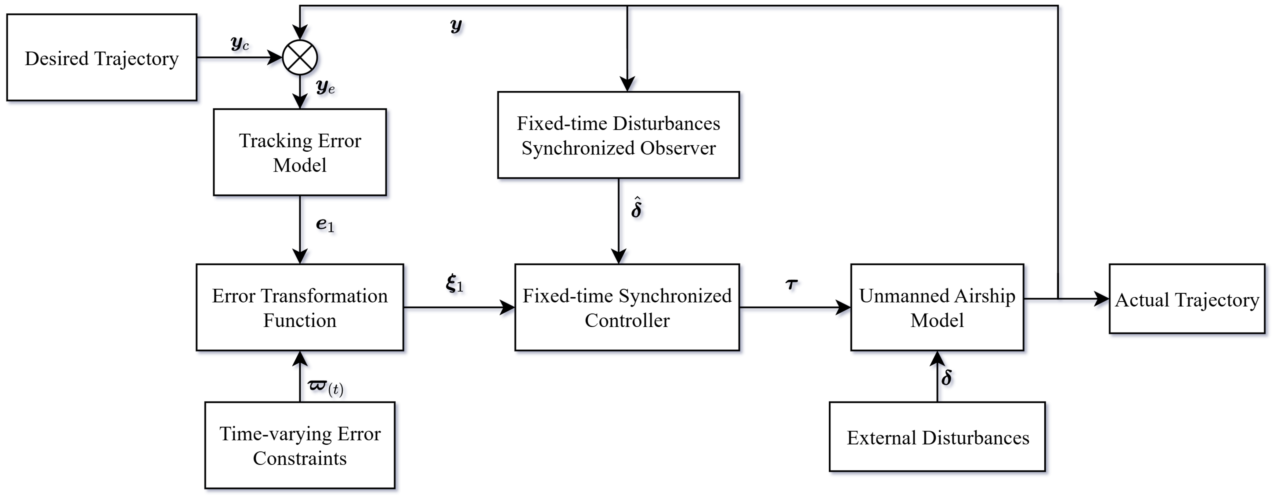
• For accurate trajectory tracking, the error should be confined to a specified range, ensuring compliance with practical performance criteria. Through the implementation of the error transformation function (ETF), the tracking errors are systematically transformed, enforcing tracking errors strictly confined in prescribed time-varying error boundaries throughout the tracking process.
• Distinct from conventional nonlinear control approaches that are irrespective of synchronization of each state convergence, built upon the Norm-Normalized sign (NNS) function, this work establishes a control algorithm, effectively ensuring simultaneous stabilization of all tracking error and estimation error components.
• In contrast to DOs that solely ensure fixed-time disturbance estimation, this work proposes a fixed-time synchronized disturbance observer (FTSDO) to achieve the exact reconstruction of uncertain disturbances while guaranteeing the synchronous fixed-time convergence of all estimation errors.

This work is organized as follows. Fundamental definitions and supporting mathematical lemmas are systematically organized in Section 2. Encompassing model transformation processes and articulating the control objective, Section 3 introduces the detailed dynamical model of the airship. Section 4 concentrates on establishing the FTSDO and designing tracking control scheme for the airship. To experimentally confirm the performance of the established control algorithm, comprehensive graphical simulations are described in Section 5. The principal contributions and delineated prospective research directions are consolidated in Section 6.

2. Preliminaries

Definition 1. 

In accordance with the theories in [22], based on

$${\mathit{sign}}_{\mathrm{n}}\left(\mathit{z}\right)\triangleq \left\{\begin{array}{cc}{\displaystyle \frac{\mathit{z}}{\parallel \mathit{z}\parallel }},\hfill & \mathit{z}\ne 0,\hfill \\ 0,\hfill & \mathit{z}=0.\hfill \end{array}\right.$$

(1)

the NNS function $\mathit{sig}\left(\mathit{z}\right)$ in this paper is introduced as follows:

$$\begin{array}{c}\hfill \begin{array}{cc}\hfill & {\mathit{sig}}^n\left(\mathit{z}\right)={\parallel \mathit{z}\parallel }^n{\mathit{sign}}_n\left(\mathit{z}\right)\hfill \end{array}\end{array}$$

(2)

where $\mathit{z}\in {\mathbb{R}}^n$ and ${\mathit{sig}}^n\left(\mathit{z}\right)$ are continuous for $n>0$.

Lemma 1 

([35]). Consider a nonlinear dynamical system expressed as $\dot{\mathit{z}}=\mathcal{F}\left(\mathit{z}\left(t\right)\right),\mathit{z}\left(0\right)={\mathit{z}}_0$, where $\mathit{z}\in {\mathbb{R}}^n$, and $\mathcal{F}(0,t)=0,\forall t\ge 0$. This system exhibits fixed-time stability if a Lyapunov function candidate $V\left(\mathit{z}\right)$ can be selected to fulfill the following inequality

$$\dot{V}\left(\mathit{z}\right)\le -{\left({\gamma }_1{V}^a\left(\mathit{z}\right)+{\gamma }_2{V}^b\left(\mathit{z}\right)\right)}^{\rho }$$

(3)

where $\{{\gamma }_1,{\gamma }_2,a,b,\rho \}>0$, $b\rho >1$, and $a\rho <1$. The convergence time $T_1$ can be expressed as follows:

$$T_1\le {\displaystyle \frac{1}{{\gamma }_1^{\rho }(1-a\rho )}}+{\displaystyle \frac{1}{{\gamma }_2^{\rho }(b\rho -1)}}$$

(4)

Lemma 2 

([36]). For the nonlinear system analyzed in Lemma 1, the system exhibits fixed-time synchronized stability (FTSS) with the convergence time

$$T_2\le {\displaystyle \frac{1}{{\gamma }_1^{\rho }(1-a\rho )}}+{\displaystyle \frac{1}{{\gamma }_2^{\chi }(b\rho -1)}}$$

(5)

provided that the conditions stated below are fulfilled:

1. 

The same constants ${\gamma }_1,{\gamma }_2,a,b,\rho$, and $V\left(\mathit{z}\right)$ in Lemma 1 satisfy the inequality in (3).

2. 

The system state $\mathit{z}$ maintains ratio persistence:

$${\displaystyle \frac{\mathit{z}}{\parallel \mathit{z}\parallel }}=\eta {\displaystyle \frac{\mathcal{Y}\left(\mathit{z}\right)}{\parallel \mathcal{Y}\left(\mathit{z}\right)\parallel }}$$

(6)

where $\eta \in \{+1,-1\}$ denotes the direction of ratio persistence.

Lemma 3 

([37]). Consider the dynamical system described by

$$\dot{\mathit{\xi }}=-{\kappa }_1{\mathit{sig}}^r\left(\mathit{\xi }\right)-{\kappa }_2{\mathit{sig}}^s\left(\mathit{\xi }\right)$$

(7)

where $\mathit{\xi }\in {\mathbb{R}}^m$ denotes the state vector, ${\kappa }_1$, ${\kappa }_2$, r, and s are strictly positive parameters with $0<r={\displaystyle \frac{r_1}{r_2}}<1$ and $1<s={\displaystyle \frac{s_1}{s_2}}$, where $r_1$, $r_2$, $s_1$, and $s_2$ are positive odd integers. This system exhibits FTSS with the convergence time bounded by

$$T_3\le {\displaystyle \frac{2^{\frac{1-r}{2}}}{{\kappa }_1(1-r)}}+{\displaystyle \frac{2^{\frac{1-s}{2}}}{{\kappa }_2(s-1)}}$$

(8)

3. Problem Statement

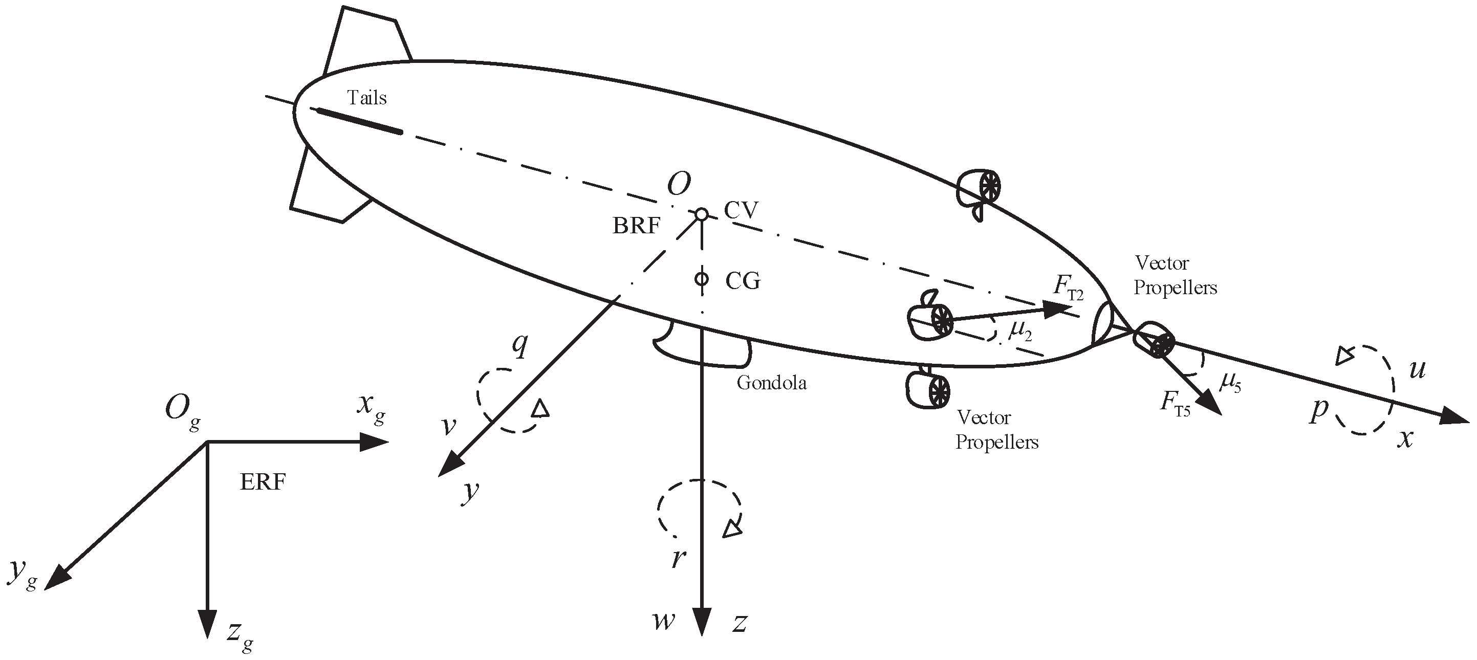
3.1. Airship Model

As depicted in Figure 1 [38], the inertial position vector $\mathit{\zeta }={\left[x,y,z\right]}^{\mathrm{T}}$ defines the vehicle’s centroid location in the Earth-fixed reference frame (ERF), while the attitude orientation $\mathit{\gamma }={\left[\varphi ,\theta ,\psi \right]}^{\mathrm{T}}$ describes its Euler angle configuration. Based on the body reference frame (BRF), the velocity components are represented by $\mathit{v}={\left[u,v,w\right]}^{\mathrm{T}}$ for translational motion and $\mathit{\omega }={\left[p,q,r\right]}^{\mathrm{T}}$ for rotational dynamics. The 6-DOF kinematic model for unmanned airships is mathematically established as

$$\left[\begin{array}{c}\dot{\mathit{\zeta }}\\ \dot{\mathit{\gamma }}\end{array}\right]=\left[\begin{array}{cc}{\mathit{R}}_{\zeta }\left(\theta ,\varphi ,\psi \right)& {\mathit{O}}_{3\times 3}\\ {\mathit{O}}_{3\times 3}& {\mathit{R}}_{\gamma }\left(\theta ,\varphi ,\psi \right)\end{array}\right]\left[\begin{array}{c}\mathit{v}\\ \mathit{\omega }\end{array}\right]$$

(9)

with

$${\mathit{R}}_{\mathit{\gamma }}(\theta ,\varphi ,\psi )=\left[\begin{array}{ccc}1& {\mathcal{T}}_{\theta }{\mathcal{S}}_{\varphi }& {\mathcal{T}}_{\theta }{\mathcal{C}}_{\varphi }\\ 0& {\mathcal{C}}_{\varphi }& -{\mathcal{S}}_{\varphi }\\ 0& {\mathcal{S}}_{\varphi }/{\mathcal{C}}_{\theta }& {\mathcal{C}}_{\varphi }/{\mathcal{C}}_{\theta }\end{array}\right]$$

(10)

and

$${\mathit{R}}_{\mathit{\zeta }}(\theta ,\varphi ,\psi )=\left[\begin{array}{ccc}{\mathcal{C}}_{\theta }{\mathcal{C}}_{\psi }& {\mathcal{S}}_{\theta }{\mathcal{C}}_{\psi }{\mathcal{S}}_{\varphi }-{\mathcal{C}}_{\varphi }{\mathcal{S}}_{\psi }& {\mathcal{S}}_{\varphi }{\mathcal{S}}_{\psi }+{\mathcal{S}}_{\theta }{\mathcal{C}}_{\psi }{\mathcal{C}}_{\varphi }\\ {\mathcal{C}}_{\theta }{\mathcal{S}}_{\psi }& {\mathcal{C}}_{\varphi }{\mathcal{C}}_{\psi }+{\mathcal{S}}_{\theta }{\mathcal{S}}_{\psi }{\mathcal{S}}_{\varphi }& -{\mathcal{S}}_{\varphi }{\mathcal{C}}_{\psi }+{\mathcal{S}}_{\theta }{\mathcal{S}}_{\psi }{\mathcal{C}}_{\varphi }\\ -{\mathcal{S}}_{\theta }& {\mathcal{C}}_{\theta }{\mathcal{S}}_{\varphi }& {\mathcal{C}}_{\theta }{\mathcal{C}}_{\varphi }\end{array}\right]$$

(11)

where ${\mathcal{S}}_{·}$, ${\mathcal{C}}_{·}$, and ${\mathcal{T}}_{·}$ denote $sin(·)$, $cos(·)$, and $tan(·)$, respectively.

Then, the dynamic model is formulated as follows:

$$\mathit{M}\left[\begin{array}{c}\dot{\mathit{v}}\\ \dot{\mathit{\omega }}\end{array}\right]+\mathit{N}=\mathit{F}+\mathit{\tau }+\mathit{\delta }$$

(12)

where

$$\mathit{M}=\left[\begin{array}{cc}m{\mathit{I}}_{3\times 3}& -m{{\mathit{r}}_C^{\prime }}^{\times }+{\mathit{M}}^{\prime }\\ m{{\mathit{r}}_C^{\prime }}^{\times }& {\mathit{I}}_O^{\prime }+{\mathit{I}}_O\end{array}\right]$$

(13)

$$\mathit{F}=\left[\begin{array}{c}{\mathit{f}}_a+{\mathit{f}}_g-{\mathit{f}}_b\\ {\mathit{m}}_a+{\mathit{m}}_g+{\mathit{m}}_b\end{array}\right]$$

(14)

$$\mathit{N}=\left[\begin{array}{c}m\mathit{\omega }\times \left(\mathit{\omega }\times {\mathit{r}}_C^{\prime }\right)+\left(m{\mathit{I}}_{3\times 3}+{\mathit{M}}^{\prime }\right)\mathit{\omega }\times \mathit{v}\\ m{\mathit{r}}_C^{\prime }\times \left(\mathit{\omega }\times \mathit{v}\right)+\mathit{\omega }\times \left({\mathit{I}}_O\mathit{\omega }\right)\end{array}\right]$$

(15)

Among the equations supplied, ${\mathit{I}}_O$ denotes the inertia matrix of the airship, and its mass is symbolized by m. The additional mass and inertia are represented by the matrices ${\mathit{M}}_O^{\prime }$ and ${\mathit{I}}_O^{\prime }$, respectively. The vector ${\mathit{r}}_C^{\prime }$ represents the displacement from the center of volume (CV) to the center of gravity (CG). Additionally, ${{\mathit{r}}_C^{\prime }}^{\times }$ represents the skew-symmetric matrix of ${\mathit{r}}_C^{\prime }$. The forces acting on the system include ${\mathit{f}}_g$, ${\mathit{f}}_b$, and ${\mathit{f}}_a$, which correspond to gravity, buoyancy, and aerodynamic forces, respectively. Similarly, ${\mathit{m}}_g$, ${\mathit{m}}_b$, and ${\mathit{m}}_a$ denote the respective torque components. The system inputs are represented by the vector $\mathit{\tau }\in {\mathbb{R}}^6$, encompassing both control forces and torques. Unknown disturbances are denoted by $\mathit{\delta }\in {\mathbb{R}}^6$. Briefly, (9) and (12) can be presented in the subsequent form:

$$\left\{\begin{array}{c}\dot{\mathit{y}}=\mathit{R}\mathit{x}\hfill \\ \mathit{M}\dot{\mathit{x}}=\mathit{F}-\mathit{N}+\mathit{\tau }+\mathit{\delta }\hfill \end{array}\right.$$

(16)

with $\mathit{y}={\left[{\mathit{\zeta }}^{\mathrm{T}},{\mathit{\gamma }}^{\mathrm{T}}\right]}^{\mathrm{T}}$, $\mathit{x}={\left[{\mathit{v}}^{\mathrm{T}},{\mathit{\omega }}^{\mathrm{T}}\right]}^{\mathrm{T}}$, and $\mathit{R}=\mathrm{diag}\{{\mathit{R}}_{\zeta },{\mathit{R}}_{\gamma }\}$.

Remark 1. 

Acknowledging the inherent challenges in modeling airship dynamics due to their large-scale configuration, significant uncertainties exist in the dynamic model. The stratospheric wind field introduces non-negligible perturbations to the system dynamics by exerting additional aerodynamic effects. Moreover, subject to current sensor technologies, real-time and precise measurements of stratospheric wind profiles face fundamental limitations. Consequently, both the inherent modeling uncertainties and wind-induced perturbations are consolidated into the disturbance $\mathit{\delta }$ in (16).

3.2. Model Transformation

The desired trajectory and velocity commands are defined as ${\mathit{y}}_c={\left[{\mathit{\zeta }}_c^{\mathrm{T}},{\mathit{\gamma }}_c^{\mathrm{T}}\right]}^{\mathrm{T}}$ and ${\mathit{x}}_c={\left[{\mathit{v}}_c^{\mathrm{T}},{\mathit{\omega }}_c^{\mathrm{T}}\right]}^{\mathrm{T}}$, respectively. Based on (11), it can be derived that

$${\mathit{R}}_{\zeta }^{-1}={\mathit{R}}_{\zeta }^{\mathrm{T}},{\dot{\mathit{R}}}_{\zeta }\left({\mathit{\gamma }}_c\right)={\mathit{R}}_{\zeta }\left({\mathit{\gamma }}_c\right)\mathit{S}\left({\mathit{\omega }}_c\right)$$

(17)

with

$$\mathit{S}\left({\mathit{\omega }}_c\right)=\left[\begin{array}{ccc}0& -r_c& q_c\\ r_c& 0& -p_c\\ -q_c& p_c& 0\end{array}\right]$$

(18)

Subsequently, the desired velocities and their derivatives can be calculated as

$$\left\{\begin{array}{c}{\mathit{v}}_c={\mathit{R}}_{\zeta }^{\mathrm{T}}\left({\mathit{\gamma }}_c\right){\dot{\mathit{\zeta }}}_c,{\dot{\mathit{v}}}_c={\mathit{R}}_{\zeta }^{\mathrm{T}}\left({\mathit{\gamma }}_c\right)\left({\ddot{\mathit{\zeta }}}_c-{\mathit{R}}_{\zeta }\left({\mathit{\gamma }}_c\right)\mathit{S}\left({\mathit{\omega }}_c\right){\mathit{v}}_c\right)\hfill \\ {\mathit{\omega }}_c={\mathit{R}}_{\gamma }^{-1}\left({\mathit{\gamma }}_c\right){\dot{\mathit{\gamma }}}_c,{\dot{\mathit{\omega }}}_c={\mathit{R}}_{\gamma }^{-1}\left({\mathit{\gamma }}_c\right)\left({\ddot{\mathit{\gamma }}}_c-{\dot{\mathit{R}}}_{\gamma }\left({\mathit{\gamma }}_c\right){\mathit{\omega }}_c\right)\hfill \end{array}\right.$$

(19)

with

$${\mathit{R}}_{\gamma }^{-1}({\theta }_c,{\varphi }_c,{\psi }_c)=\left[\begin{array}{ccc}1& 0& -{\mathcal{S}}_{{\theta }_c}\\ 0& {\mathcal{C}}_{{\varphi }_c}& {\mathcal{S}}_{{\varphi }_c}{\mathcal{C}}_{{\theta }_c}\\ 0& -{\mathcal{S}}_{{\varphi }_c}& {\mathcal{C}}_{{\varphi }_c}{\mathcal{C}}_{{\theta }_c}\end{array}\right]$$

(20)

$${\dot{\mathit{R}}}_{\gamma }({\theta }_c,{\varphi }_c,{\psi }_c)=\left[\begin{array}{ccc}0& {\displaystyle \frac{{\dot{\theta }}_c{\mathcal{S}}_{{\varphi }_c}}{{\mathcal{S}}_{{\theta }_c}^2}}+{\dot{\varphi }}_c{t}_{{\theta }_c}{\mathcal{C}}_{{\varphi }_c}& {\displaystyle \frac{{\dot{\theta }}_c{\mathcal{C}}_{{\varphi }_c}}{{\mathcal{C}}_{{\theta }_c}^2}}-{\dot{\varphi }}_c{\mathcal{T}}_{{\theta }_c}{\mathcal{S}}_{{\varphi }_c}\\ 0& -{\dot{\varphi }}_c{\mathcal{S}}_{{\varphi }_c}& -{\dot{\varphi }}_c{\mathcal{C}}_{{\varphi }_c}\\ 0& {\displaystyle \frac{{\dot{\theta }}_c{\mathcal{S}}_{{\varphi }_c}{\mathcal{S}}_{{\theta }_c}+{\dot{\varphi }}_c{\mathcal{C}}_{{\varphi }_c}{\mathcal{C}}_{{\theta }_c}}{{\mathcal{C}}_{{\theta }_c}^2}}& {\displaystyle \frac{{\dot{\theta }}_c{\mathcal{C}}_{{\varphi }_c}{\mathcal{S}}_{{\theta }_c}-{\dot{\varphi }}_c{\mathcal{S}}_{{\varphi }_c}{\mathcal{C}}_{{\theta }_c}}{{\mathcal{C}}_{{\theta }_c}^2}}\end{array}\right]$$

(21)

The position error and the attitude error are defined by ${\mathit{y}}_e=\mathit{y}-{\mathit{y}}_c$ and ${\mathit{x}}_e=\mathit{x}-{\mathit{x}}_c$, respectively, and ${\mathit{R}}_c=\mathrm{diag}\{{\mathit{R}}_{\zeta }\left({\theta }_c,{\varphi }_c,{\psi }_c\right),{\mathit{R}}_{\gamma }\left({\theta }_c,{\varphi }_c,{\psi }_c\right)\}$. Therefore, (16) can be reformulated through tracking error dynamics as

$$\left\{\begin{array}{c}{\dot{\mathit{y}}}_e=\left(\mathit{R}-{\mathit{R}}_c\right){\mathit{x}}_c+\mathit{R}{\mathit{x}}_e\hfill \\ \mathit{M}{\dot{\mathit{x}}}_e=\mathit{F}-\mathit{N}+\mathit{\tau }-\mathit{M}{\dot{\mathit{x}}}_c\hfill \end{array}\right.$$

(22)

Substituting ${\mathit{e}}_1={\mathit{y}}_e$ and ${\mathit{e}}_2={\dot{\mathit{y}}}_e$ into (22) yields the tracking error model

$$\left\{\begin{array}{c}{\dot{\mathit{e}}}_1={\mathit{e}}_2\hfill \\ {\dot{\mathit{e}}}_2=\mathit{R}{\mathit{M}}^{-1}\mathit{\delta }+\mathfrak{F}\left({\mathit{e}}_1,{\mathit{e}}_2\right)+\mathit{R}{\mathit{M}}^{-1}\mathit{\tau }\hfill \end{array}\right.$$

(23)

where

$$\begin{array}{cc}\hfill \mathfrak{F}\left({\mathit{e}}_1,{\mathit{e}}_2\right)=& \mathit{R}{\mathit{M}}^{-1}\left(\mathit{F}-\mathit{N}-\mathit{M}{\dot{\mathit{x}}}_c\right)+\left(\dot{\mathit{R}}-{\dot{\mathit{R}}}_c\right){\mathit{x}}_c\hfill \\ \hfill & +\left(\mathit{R}-{\mathit{R}}_c\right){\dot{\mathit{x}}}_c-\dot{\mathit{R}}{\mathit{R}}^{-1}\left(\mathit{R}-{\mathit{R}}_c\right){\mathit{x}}_c+\dot{\mathit{R}}{\mathit{R}}^{-1}{\mathit{e}}_2\hfill \end{array}$$

(24)

3.3. Control Objective

The architecture of the proposed control scheme is presented in Figure 2. The control objective involves synthesizing a control input $\mathit{\tau }$ for system (23) to ensure the airship accurately follows the reference trajectory ${\mathit{y}}_c$. Specifically, the tracking error ${\mathit{e}}_1$ is required to be driven to a small, bounded vicinity of the origin in fixed time, while strictly adhering to prescribed time-varying constraint boundaries throughout the convergence process. Moreover, the convergence of all components of ${\mathit{e}}_1$ should be achieved synchronously.

4. Main Results

4.1. Fixed-Time Synchronized Observer Design

To precisely estimate the disturbances in (23), an FTSDO was constructed as follows.

For this target, we began by reformulating the tracking error dynamics as

$${\dot{\mathit{e}}}_2=-k_1{\mathit{e}}_2+\mathit{R}{\mathit{M}}^{-\mathbf{1}}\mathit{\tau }+{\mathit{\delta }}^{\ast }$$

(25)

where the synthesized disturbance term ${\mathit{\delta }}^{\ast }$ was expressed as

$${\mathit{\delta }}^{\ast }=k_1{\mathit{e}}_2+\mathfrak{F}({\mathit{e}}_1,{\mathit{e}}_2)+\mathit{R}{\mathit{M}}^{-\mathbf{1}}\mathit{\delta }$$

(26)

with $k_1>0$. Following the structure of (25), an auxiliary state variable ${\dot{\widehat{\mathit{e}}}}_2$ was established

$${\dot{\widehat{\mathit{e}}}}_2=-k_1{\widehat{\mathit{e}}}_2+\mathit{R}{\mathit{M}}^{-1}\mathit{\tau }$$

(27)

Subsequently, using two intermediate variables ${\mathit{s}}_1={\mathit{e}}_2-{\widehat{\mathit{e}}}_2$ and ${\mathit{s}}_2=k_2{\mathit{s}}_1$ (where $k_2>0$), substituting (25) and (27) into ${\mathit{s}}_1$, the dynamic system could be transformed to

$$\left\{\begin{array}{c}{\dot{\mathit{s}}}_1=-k_1{\mathit{s}}_1+{\mathit{\delta }}^{\ast }\hfill \\ {\mathit{s}}_2=k_2{\mathit{s}}_1\hfill \end{array}\right.$$

(28)

Following the formulations (25)–(28), the FTSDO was as follows:

$$\left\{\begin{array}{l}{\dot{\widehat{\mathit{s}}}}_1={\displaystyle \frac{{\dot{\mathit{s}}}_2}{k_2}}+{\alpha }^{\ast }{sig}^{p^{\ast }}\left({\tilde{\mathit{s}}}_1\right)+{\beta }^{\ast }{sig}^{g^{\ast }}\left({\tilde{\mathit{s}}}_1\right)\hfill \\ {\widehat{\delta }}^{\ast }={\displaystyle \frac{k_1{k}_2{\widehat{\mathit{s}}}_1+{\dot{\mathit{s}}}_2}{k_2}}\hfill \\ \widehat{\delta }=\mathit{M}{\mathit{R}}^{-1}\left({\widehat{\delta }}^{\ast }-k_1{\mathit{e}}_2-\mathfrak{F}\left({\mathit{e}}_1,{\mathit{e}}_2\right)\right)\hfill \end{array}\right.$$

(29)

where ${\tilde{\mathit{s}}}_1={\mathit{s}}_1-{\widehat{\mathit{s}}}_1$, $\{k_2$, ${\alpha }^{\ast }$, ${\beta }^{\ast }\}>0$, and $p^{\ast }$ and $g^{\ast }$ satisfy similar conditions as r and s in Lemma 3.

Theorem 1. 

By appropriately selecting the parameters $k_1$, $k_2$, ${\alpha }^{\ast }$, ${\beta }^{\ast }$, $p^{\ast }$, and $g^{\ast }$, the FTSDO (29) can guarantee that all estimation error components $\tilde{\mathit{\delta }}=\mathit{\delta }-\widehat{\mathit{\delta }}$ achieve fixed-time synchronous convergence to a compact region containing the origin, and there exists $T_{\delta }>0$, $\forall t\ge T_{\delta }$, the inequality $\parallel \tilde{\mathit{\delta }}\parallel \le {\mathit{ϵ}}^{\ast }$ holds, where ${\mathit{ϵ}}^{\ast }$ can be driven to an arbitrarily small value through proper parameter selection.

Proof of Theorem 1. 

Substituting (28) and (29) into the derivative of $\tilde{\mathit{s}}$, the following results are obtained

$$\begin{array}{cc}\hfill {\dot{\tilde{\mathit{s}}}}_1& ={\dot{\mathit{s}}}_1-{\dot{\widehat{\mathit{s}}}}_1\hfill \\ \hfill & ={\dot{\mathit{s}}}_1-{\displaystyle \frac{{\dot{\mathit{s}}}_2}{k_2}}-{\alpha }^{\ast }{\mathrm{sig}}^{p^{\ast }}\left({\tilde{\mathit{s}}}_1\right)-{\beta }^{\ast }{\mathrm{sig}}^{g^{\ast }}\left({\tilde{\mathit{s}}}_1\right)\hfill \\ \hfill & =-{\alpha }^{\ast }{\mathrm{sig}}^{p^{\ast }}\left({\tilde{\mathit{s}}}_1\right)-{\beta }^{\ast }{\mathrm{sig}}^{g^{\ast }}\left({\tilde{\mathit{s}}}_1\right)\hfill \end{array}$$

(30)

According to Lemma 3, ${\tilde{\mathit{s}}}_1$ is FTSS with the convergence time $T_{\delta }$ calculated by (8).

Then, combining (26) with (29), the estimation error $\tilde{\mathit{\delta }}$ admits a representation

$$\begin{array}{cc}\hfill \tilde{\mathit{\delta }}& =\mathit{M}{\mathit{R}}^{-1}\left({\mathit{\delta }}^{\ast }-{\widehat{\mathit{\delta }}}^{\ast }\right)\hfill \\ \hfill & =\mathit{M}{\mathit{R}}^{-1}\left({\mathit{\delta }}^{\ast }-{\displaystyle \frac{k_1{k}_2{\widehat{\mathit{s}}}_1-k_1{k}_2{\mathit{s}}_1+k_2{\mathit{\delta }}^{\ast }}{k_2}}\right)\hfill \\ \hfill & =k_1\mathit{M}{\mathit{R}}^{-1}{\tilde{\mathit{s}}}_1\hfill \end{array}$$

(31)

By invoking (30) and (31), it follows that the estimation error $\tilde{\mathit{\delta }}$ also achieves synchronous convergence to a small region around zero for all $t>T_{\mathit{\delta }}$. This inherently demonstrates that all components of the disturbance $\mathit{\delta }$ are synchronously reconstructed by its estimation $\widehat{\mathit{\delta }}$ in fixed time. This brings the proof to its completion. □

4.2. Fixed-Time Synchronized Controller Design

In this section, a fixed-time synchronized controller (denoted as FTSS controller) based on the ETF is developed. The disturbance $\mathit{\delta }$ is estimated by the FTSDO constructed in Section 4.1. The design of the FTSS controller follows a backstepping procedure, which is detailed in the following.

Definition 2 

([28]). A smooth function ${\mathbb{F}}_i\left({\mathit{ϵ}}_i\right)$, where i is a positive integer, is termed an ETF if it fulfills the subsequent conditions:

1. 

Smooth, monotonically increasing;

2. 

$-1<{\mathbb{F}}_i\left({\mathit{ϵ}}_i\right)<1$;

3. 

${lim}_{{\mathit{ϵ}}_i\to -\infty }{\mathbb{F}}_i\left({\mathit{ϵ}}_i\right)=-1$, ${lim}_{{\mathit{ϵ}}_i\to +\infty }{\mathbb{F}}_i\left({\mathit{ϵ}}_i\right)=1$;

where ${\mathit{ϵ}}_i$ is the transformed error.

Combining the airship tracking error model with the error transformation function based on Definition 2, an error transformation function can be selected as

$$\mathbb{F}\left({\mathit{ϵ}}_{\mathbf{1}}\right)={\displaystyle \frac{{\mathit{e}}_1}{{\mathit{\varpi }}_{\left(t\right)}}}={\displaystyle \frac{2}{\pi }}arctan\left({\mathit{ϵ}}_1\right)$$

(32)

with time-varying constraint boundary ${\mathit{\varpi }}_{\left(t\right)}$ predefined as ${\mathit{\varpi }}_{\left(t\right)}={\mathbf{\Omega }}_t^{\ast }+({\mathbf{\Omega }}_0-{\mathbf{\Omega }}_t^{\ast })exp(-\mathit{\lambda }t)$, and ${\mathbf{\Omega }}_t^{\ast }$, ${\mathbf{\Omega }}_0$, and $\mathit{\lambda }$ are predefined constant vectors.

Consequently, the transformed error ${\mathit{ϵ}}_1$ is given by

$${\mathit{ϵ}}_1={\mathbb{F}}^{-1}\left({\displaystyle \frac{{\mathit{e}}_1}{{\mathit{\varpi }}_{\left(t\right)}}}\right)=tan\left({\displaystyle \frac{\pi {\mathit{e}}_1}{2{\mathit{\varpi }}_{\left(t\right)}}}\right)$$

(33)

where $|{\mathit{e}}_1|$ is bounded by $|{\mathit{e}}_{1\left(0\right)}|\le |{\mathit{\varpi }}_{\left(0\right)}|$.

To implement the backstepping control design, two intermediate variables ${\mathit{\xi }}_1$ and ${\mathit{\xi }}_2$ are defined as

$$\left\{\begin{array}{c}{\mathit{\xi }}_1=tan\left({\displaystyle \frac{\pi {\mathit{e}}_1}{2{\mathit{\varpi }}_{\left(t\right)}}}\right)\hfill \\ {\mathit{\xi }}_2={\mathit{e}}_2-{\mathit{e}}_2^{\ast }\hfill \end{array}\right.$$

(34)

$\mathit{Step}$ 1. For the purpose of facilitating the subsequent controller design, the intermediate control law ${\mathit{e}}_2^{\ast }$ can be selected as

$${\mathit{e}}_2^{\ast }={\displaystyle \frac{{\mathit{e}}_1{\dot{\mathit{\varpi }}}_{\left(t\right)}}{{\mathit{\varpi }}_{\left(t\right)}}}+{\mathit{\Omega }}^{-1}{\mathit{\psi }}_1$$

(35)

with

$${\mathit{\psi }}_1=-{\alpha }_1{\mathrm{sig}}^{p_1}\left({\mathit{\xi }}_1\right)-{\beta }_1{\mathrm{sig}}^{g_1}\left({\mathit{\xi }}_1\right)$$

(36)

where ${\alpha }_1$, ${\beta }_1$, $p_1$, and $g_1$ are chosen as constants similar to ${\kappa }_1$, ${\kappa }_2$, r, and s, respectively, in Lemma 3.

According to (33) and (34), the derivative of ${\mathit{\xi }}_1$ can be calculated as

$${\dot{\mathit{\xi }}}_1=\mathit{\Omega }\left({\dot{\mathit{e}}}_1-{\displaystyle \frac{{\mathit{e}}_1{\dot{\mathit{\varpi }}}_{\left(t\right)}}{{\mathit{\varpi }}_{\left(t\right)}}}\right)$$

(37)

where $\mathit{\Omega }={\displaystyle \frac{\pi }{2{\mathit{\varpi }}_{\left(t\right)}}}{sec}^2\left({\displaystyle \frac{\pi {\mathit{e}}_1}{2{\mathit{\varpi }}_{\left(t\right)}}}\right)$.

Integrating (35) with (37) establishes

$${\dot{\mathit{\xi }}}_1=\mathit{\Omega }{\mathit{\xi }}_2+{\mathit{\psi }}_1$$

(38)

For the stability of ${\mathit{\xi }}_1$, a Lyapunov function can be chosen as follows:

$$V_1=\sum _{i=1}^6{\displaystyle \frac{1}{2}}{\xi }_{1i}^{\mathrm{T}}{\xi }_{1i}$$

(39)

Combining (38) with (39), the derivative of $V_1$ is obtained through calculation as

$${\dot{V}}_1=\sum _{i=1}^6{\xi }_{1i}^{\mathrm{T}}{\dot{\xi }}_{1i}=\sum _{i=1}^6{\xi }_{1i}^{\mathrm{T}}{\Omega }_i{\xi }_{2i}+\sum _{i=1}^6{\xi }_{1i}^{\mathrm{T}}{\psi }_{1i}$$

(40)

where ${\xi }_{1i}$ and ${\dot{\xi }}_{1i}$ are the ith element of ${\mathit{\xi }}_1$ and its derivatives ${\dot{\mathit{\xi }}}_1$, respectively; ${\psi }_{1i}$ and ${\Omega }_i$ are the ith element of ${\mathit{\psi }}_1$ and $\mathit{\Omega }$.

$\mathit{Step}$ 2. Subsequently, for the purpose of stabilizing ${\mathit{\xi }}_1$ and ${\mathit{\xi }}_2$, the control input $\mathit{\tau }$ takes the following form

$$\begin{array}{cc}\hfill \mathit{\tau }=& \mathit{M}{\mathit{R}}^{-1}\left(-\mathfrak{F}\left({\mathit{e}}_1,{\mathit{e}}_2\right)+{\displaystyle \frac{({\dot{\mathit{e}}}_1{\dot{\mathit{\varpi }}}_{\left(t\right)}+{\mathit{e}}_1{\ddot{\mathit{\varpi }}}_{\left(t\right)}){\mathit{\varpi }}_{\left(t\right)}-{\mathit{e}}_1{\dot{\mathit{\varpi }}}_{\left(t\right)}^2}{{\mathit{\varpi }}_{\left(t\right)}^2}}\right.\hfill \\ \hfill & \left.+{\displaystyle \frac{{\dot{\mathit{\psi }}}_1\mathit{\Omega }-{\mathit{\psi }}_1\dot{\mathit{\Omega }}}{{\mathit{\Omega }}^2}}+{\mathit{\psi }}_2-\mathit{R}{\mathit{M}}^{-1}\widehat{\mathit{\delta }}\right)\hfill \end{array}$$

(41)

where

$$\dot{\mathit{\Omega }}={\displaystyle \frac{\pi {\mathit{e}}_1}{2{\mathit{\varpi }}^2\left(t\right)}}\left(-{sec}^2\left({\displaystyle \frac{\pi {\mathit{e}}_1}{2{\mathit{\varpi }}_{\left(t\right)}}}\right)+{sec}^2\left({\displaystyle \frac{\pi {\mathit{e}}_1}{2{\mathit{\varpi }}_{\left(t\right)}}}\right)tan\left({\displaystyle \frac{\pi {\mathit{e}}_1}{2{\mathit{\varpi }}_{\left(t\right)}}}\right)·{\mathit{\varrho }}^{\ast }\right)$$

(42)

with

$${\mathit{\varrho }}^{\ast }={\displaystyle \frac{{\dot{\mathit{e}}}_1}{{\mathit{\varpi }}_{\left(t\right)}}}-{\displaystyle \frac{{\mathit{e}}_1{\dot{\mathit{\varpi }}}_{\left(t\right)}}{{\mathit{\varpi }}_{\left(t\right)}^2}}$$

(43)

$$\begin{array}{cc}\hfill {\mathit{\psi }}_2& =-{\alpha }_2{\mathrm{sig}}^{p_2}\left({\mathit{\xi }}_2\right)-{\beta }_2{\mathrm{sig}}^{g_2}\left({\mathit{\xi }}_2\right),\hfill \end{array}$$

(44)

$$\begin{array}{cc}\hfill {\dot{\mathit{\psi }}}_1& =-\left({\mathit{\rho }}_1{\mathit{\xi }}_1{\mathit{\xi }}_1^{\mathrm{T}}{\dot{\mathit{\xi }}}_1+{\mathit{\rho }}_2{\dot{\mathit{\xi }}}_1\right),\hfill \end{array}$$

(45)

with

$${\mathit{\rho }}_1={\alpha }_1(p_1-1){\mathit{\xi }}_1^{p_1-3}+{\beta }_1(g_1-1){\mathit{\xi }}_1^{g_1-3},$$

(46)

$${\mathit{\rho }}_2={\alpha }_1{\mathit{\xi }}_1^{p_1-1}+{\beta }_1{\mathit{\xi }}_1^{g_1-1}$$

(47)

In this step, the following Lyapunov function is selected as follows:

$$V_2=\sum _{i=1}^6{\displaystyle \frac{1}{2}}{\xi }_{2i}^{\mathrm{T}}{\xi }_{2i}$$

(48)

where ${\xi }_{2i}$ is the ith element of ${\mathit{\xi }}_2$.

Through the synthesis of (23), (34), and (35), the derivative of ${\mathit{\xi }}_2$ is derived as

$$\begin{array}{cc}\hfill {\dot{\mathit{\xi }}}_2& =\mathfrak{F}\left({\mathit{e}}_1,{\mathit{e}}_2\right)+\mathit{R}{\mathit{M}}^{-1}\mathit{\tau }-{\displaystyle \frac{({\dot{\mathit{e}}}_1{\dot{\mathit{\varpi }}}_{\left(t\right)}+{\mathit{e}}_1{\ddot{\mathit{\varpi }}}_{\left(t\right)}){\mathit{\varpi }}_{\left(t\right)}-{\mathit{e}}_1{\dot{\mathit{\varpi }}}_{\left(t\right)}^2}{{\mathit{\varpi }}_{\left(t\right)}^2}}\hfill \\ \hfill & -{\displaystyle \frac{{\dot{\mathit{\psi }}}_1\mathit{\Omega }-{\mathit{\psi }}_1\dot{\mathit{\Omega }}}{{\mathit{\Omega }}^2}}+\mathit{R}{\mathit{M}}^{-1}\mathit{\delta }\hfill \end{array}$$

(49)

By applying equations (41) and (49), it follows that

$${\dot{\mathit{\xi }}}_2={\mathit{\psi }}_2+\mathit{R}{\mathit{M}}^{-1}\tilde{\mathit{\delta }}$$

(50)

Combining (48), (49), and (50), we can obtain

$$\begin{array}{cc}\hfill {\dot{V}}_2& =\sum _{i=1}^6{\xi }_{1i}^{\mathrm{T}}{\mathsf{\Omega }}_i{\xi }_{2i}+\sum _{i=1}^6{\xi }_{1i}^{\mathrm{T}}{\psi }_{1i}+\sum _{i=1}^6{\xi }_{2i}^{\mathrm{T}}{\dot{\xi }}_{2i}\hfill \\ \hfill & =\sum _{i=1}^6{\xi }_{1i}^{\mathrm{T}}{\mathsf{\Omega }}_i{\xi }_{2i}+\sum _{i=1}^6{\xi }_{1i}^{\mathrm{T}}{\psi }_{1i}+\sum _{i=1}^6{\xi }_{2i}^{\mathrm{T}}{\psi }_{2i}+{\mathit{\xi }}_2^{\mathrm{T}}\mathit{R}{\mathit{M}}^{-1}\tilde{\mathit{\delta }}\hfill \end{array}$$

(51)

where ${\dot{\xi }}_{2i}$ and ${\psi }_{2i}$ are the ith element of ${\dot{\mathit{\xi }}}_2$ and ${\mathit{\psi }}_2$, respectively.

Remark 2 

([22]). The derivative calculations referenced in (46) adhere to the following rules

$${\displaystyle \frac{\partial }{\partial \mathit{\xi }}}{\mathit{sig}}^{p+1}\left(\mathit{\xi }\right)=p{∥\mathit{\xi }∥}^{p-2}\mathit{\xi }{\mathit{\xi }}^{\mathrm{T}}+{∥\mathit{\xi }∥}^p{\mathit{I}}_m$$

(52)

$${\displaystyle \frac{\partial }{\partial \mathit{\xi }}}{∥\mathit{\xi }∥}^{p+1}=(p+1){∥\mathit{\xi }∥}^{p-1}\mathit{\xi }$$

(53)

$${\displaystyle \frac{\partial }{\partial t}}{∥\mathit{\xi }∥}^{p+1}=(p+1){∥\mathit{\xi }∥}^{p-1}{\mathit{\xi }}^T\dot{\mathit{\xi }}$$

(54)

where the state vector $\mathit{\xi }\in {\mathbb{R}}^m$, and the constant $n\in \mathbb{R}$.

4.3. Stability Analysis

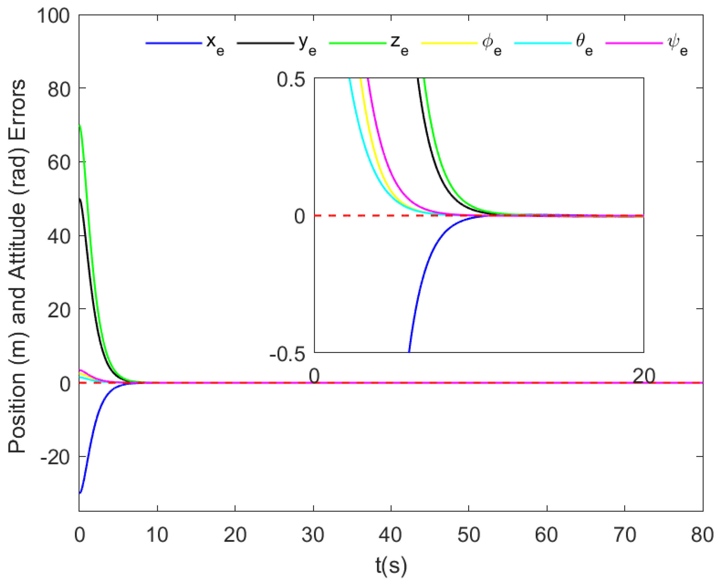
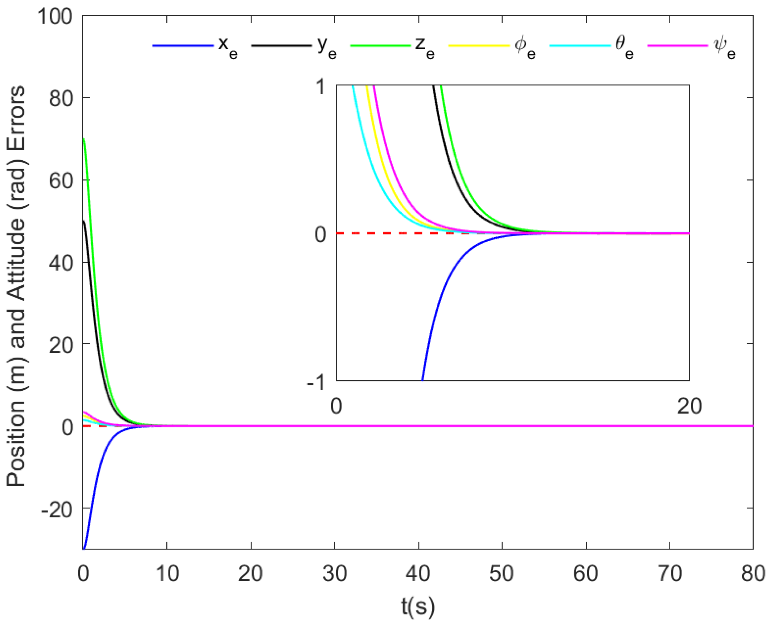
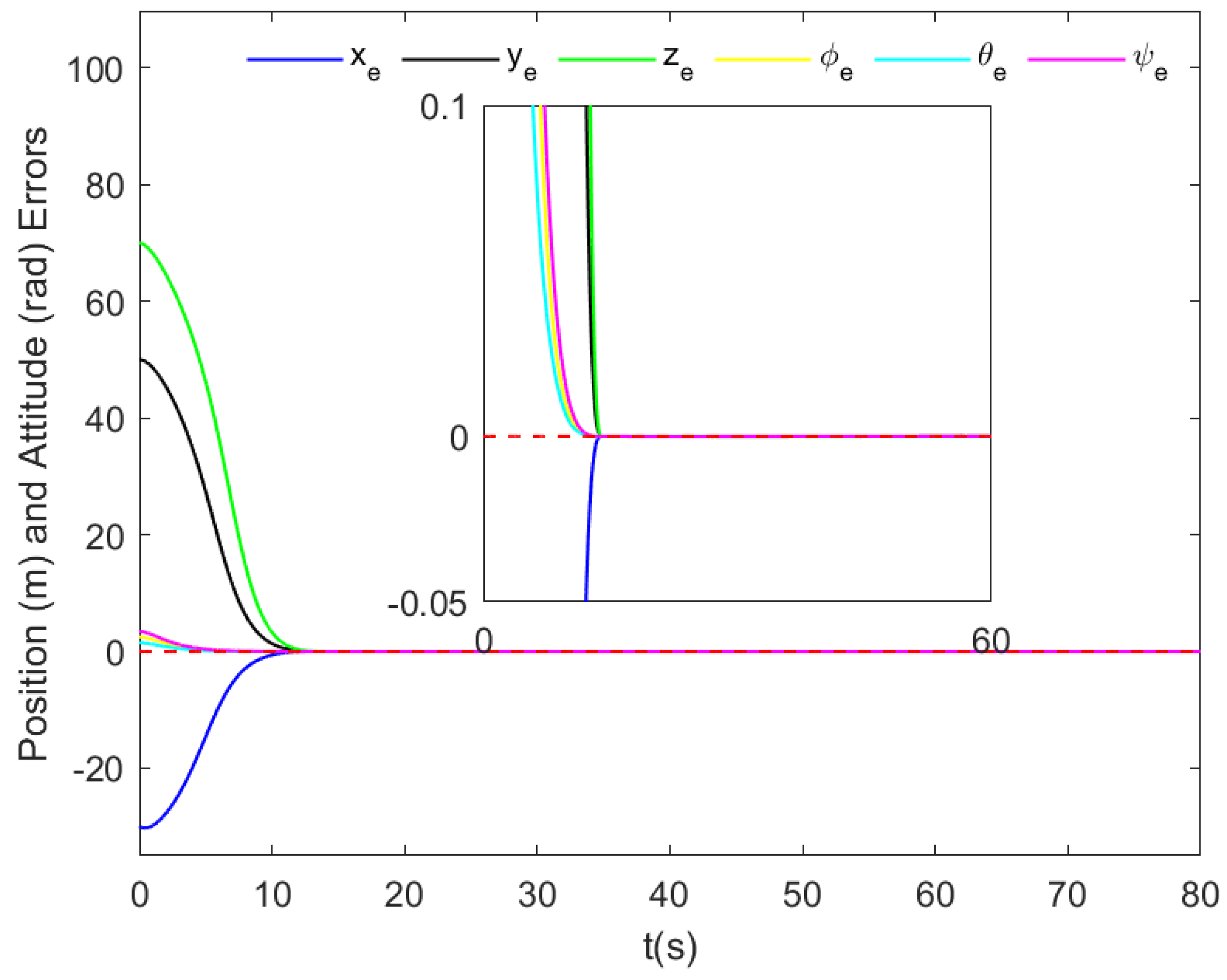
Theorem 2. 

Considering the error-constrained system (23) with predetermined constraint boundaries ${\mathit{\varpi }}_{\left(t\right)}$ and unknown disturbances $\mathit{\delta }$, the FTSDO (29) and control law (41) are developed. By appropriately selecting the design parameters ${\alpha }_1,{\alpha }_2,{\beta }_1,{\beta }_2,p_1,p_2,g_1$, and $g_2$, the proposed control law $\mathit{\tau }$ guarantees all components of tracking error vectors ${\mathit{e}}_1$ simultaneously converge to a small region around zero in fixed time without violating the error constraint ${\mathit{\varpi }}_{\left(t\right)}$.

Proof of Theorem 2. 

Inspired by the aforementioned analysis, the Lyapunov function can be finally selected as

$$V=V_1+V_2=\sum _{i=1}^6{\displaystyle \frac{1}{2}}{\xi }_{1i}^{\mathrm{T}}{\xi }_{1i}+\sum _{i=1}^6{\displaystyle \frac{1}{2}}{\xi }_{2i}^{\mathrm{T}}{\xi }_{2i}$$

(55)

By integrating (40), (51), and (55), the following can be obtained

$$\dot{V}=\sum _{i=1}^6{\xi }_{1i}^{\mathrm{T}}{\dot{\xi }}_{1i}+\sum _{i=1}^6{\xi }_{2i}^{\mathrm{T}}{\dot{\xi }}_{2i}$$

(56)

Combining (40) and (51) with (56) yields

$$\dot{V}=\sum _{i=1}^6{\xi }_{1i}^{\mathrm{T}}{\Omega }_i{\xi }_{2i}+\sum _{i=1}^6{\xi }_{1i}^{\mathrm{T}}{\psi }_{1i}+\sum _{i=1}^6{\xi }_{2i}^{\mathrm{T}}{\psi }_{2i}+{\mathit{\xi }}_2^{\mathrm{T}}\mathit{R}{\mathit{M}}^{-1}\tilde{\mathit{\delta }}$$

(57)

Inserting (36) and (44) into (57) leads to

$$\begin{array}{cc}\hfill \dot{V}& =\sum _{i=1}^6{\xi }_{1i}^{\mathrm{T}}{\Omega }_i{\xi }_{2i}-\sum _{i=1}^6{\alpha }_1{∥{\xi }_{1i}∥}^{1+p_1}-\sum _{i=1}^6{\beta }_1{∥{\xi }_{1i}∥}^{1+g_1}\hfill \\ \hfill & -\sum _{i=1}^6{\alpha }_2{∥{\xi }_{2i}∥}^{1+p_2}-\sum _{i=1}^6{\beta }_2{∥{\xi }_{2i}∥}^{1+g_2}+{\mathit{\xi }}_2^{\mathrm{T}}\mathit{R}{\mathit{M}}^{-1}\tilde{\mathit{\delta }}\hfill \end{array}$$

(58)

Through the application of Young’s inequality, we derive that

$$\begin{array}{cc}\hfill \dot{V}& \le {\displaystyle \frac{{\left({\mathsf{\Omega }}_i^{\ast }\right)}^2}{2}}\left(\sum _{i=1}^6\parallel {\xi }_{1i}{\parallel }^{1+g_1}+\sum _{i=1}^6{\parallel {\xi }_{2i}\parallel }^{1+g_2}\right)-\sum _{i=1}^6{\alpha }_1\parallel {\xi }_{1i}{\parallel }^{1+p_1}-\sum _{i=1}^6{\beta }_1{\parallel {\xi }_{1i}\parallel }^{1+g_1}\hfill \\ \hfill & -\sum _{i=1}^6{\alpha }_2\parallel {\xi }_{2i}{\parallel }^{1+p_2}-\sum _{i=1}^6{\beta }_2{\parallel {\xi }_{2i}\parallel }^{1+g_2}+{\mathit{\xi }}_2^{\mathrm{T}}\mathit{R}{\mathit{M}}^{-1}\tilde{\mathit{\delta }}\hfill \\ \hfill & \le -\sum _{i=1}^6{\alpha }_1\parallel {\xi }_{1i}{\parallel }^{1+p_1}-\sum _{i=1}^6{\alpha }_2\parallel {\xi }_{2i}{\parallel }^{1+p_2}-\sum _{i=1}^6{\gamma }_1{\parallel {\xi }_{1i}\parallel }^{1+g_1}\hfill \\ \hfill & -\sum _{i=1}^6{\gamma }_2{\parallel {\xi }_{2i}\parallel }^{1+g_2}+{\mathit{\xi }}_2^{\mathrm{T}}\mathit{R}{\mathit{M}}^{-1}\tilde{\mathit{\delta }}\hfill \end{array}$$

(59)

where ${\Omega }_i^{\ast }=max\{{\Omega }_i,1\}$, ${\gamma }_1={\beta }_1-{\displaystyle \frac{{\left({\Omega }_i^{\ast }\right)}^2}{2}}$, and ${\gamma }_2={\beta }_2-{\displaystyle \frac{{\left({\Omega }_i^{\ast }\right)}^2}{2}}$.

The parameters are defined as follows:

$p=min\{p_1,p_2\}$, $g=min\{g_1,g_2\}$, $\alpha =min\{{\alpha }_1,{\alpha }_2\}$, $\beta =min\{{\gamma }_1,{\gamma }_2\}$

Through rigorous analysis, we demonstrate that

$$\begin{array}{cc}\hfill \dot{V}& \le -{\alpha }_1{V}_1^{{\displaystyle \frac{1+p}{2}}}-{\alpha }_2{V}_2^{{\displaystyle \frac{1+p}{2}}}-{\gamma }_1{V}_1^{{\displaystyle \frac{1+g}{2}}}-{\gamma }_2{V}_2^{{\displaystyle \frac{1+g}{2}}}+{\mathit{\xi }}_2^{\mathrm{T}}\mathit{R}{\mathit{M}}^{-1}\tilde{\mathit{\delta }}\hfill \\ \hfill & \le -\alpha V^{{\displaystyle \frac{1+p}{2}}}-\beta V^{{\displaystyle \frac{1+g}{2}}}+{\mathit{\xi }}_2^{\mathrm{T}}\mathit{R}{\mathit{M}}^{-1}\tilde{\mathit{\delta }}\hfill \end{array}$$

(60)

• Based on Theorem 1, $\parallel \tilde{\mathit{\delta }}\parallel \le {ϵ}^{\ast }$, for all $t\ge T_{\delta }$, and ${ϵ}^{\ast }$ is arbitrarily small. Therefore, all tracking errors are fixed-time stable according to Lemma 1. Combining (50) with Lemma 3, ${\mathit{\psi }}_2$ exhibits FTSS with the convergence time $T_{h_2}$. Then, from (38), we have $\dot{{\mathit{\xi }}_{\mathbf{1}}}={\mathit{\psi }}_1$, and ${\mathit{e}}_1$ and ${\mathit{e}}_2$ achieve synchronized stability with the convergence time $T_{h_1}$. Consequently, $\forall t>T_{h_1}+T_{h_2}+T_{\delta }$, all tracking errors exhibit FTSS.
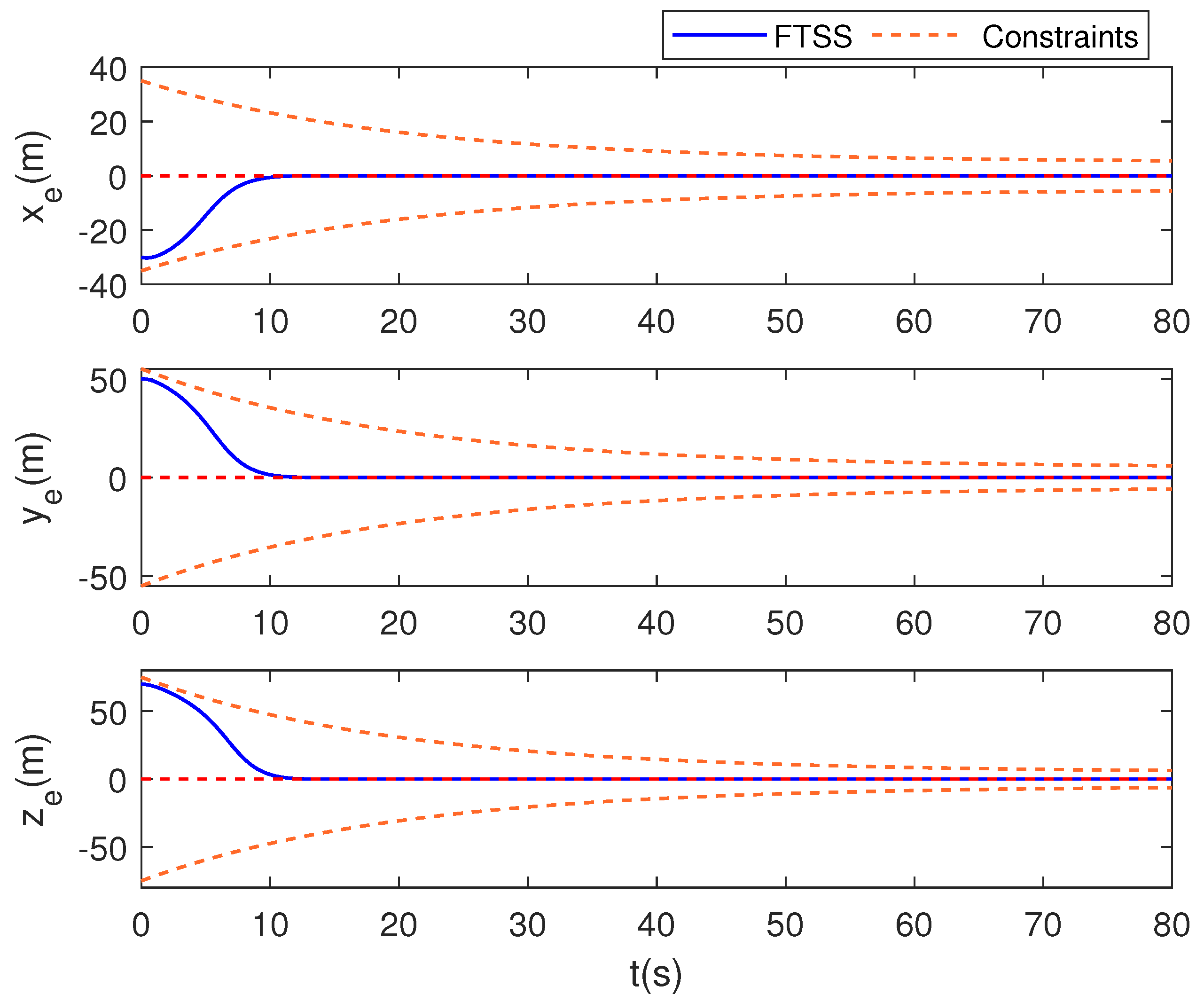
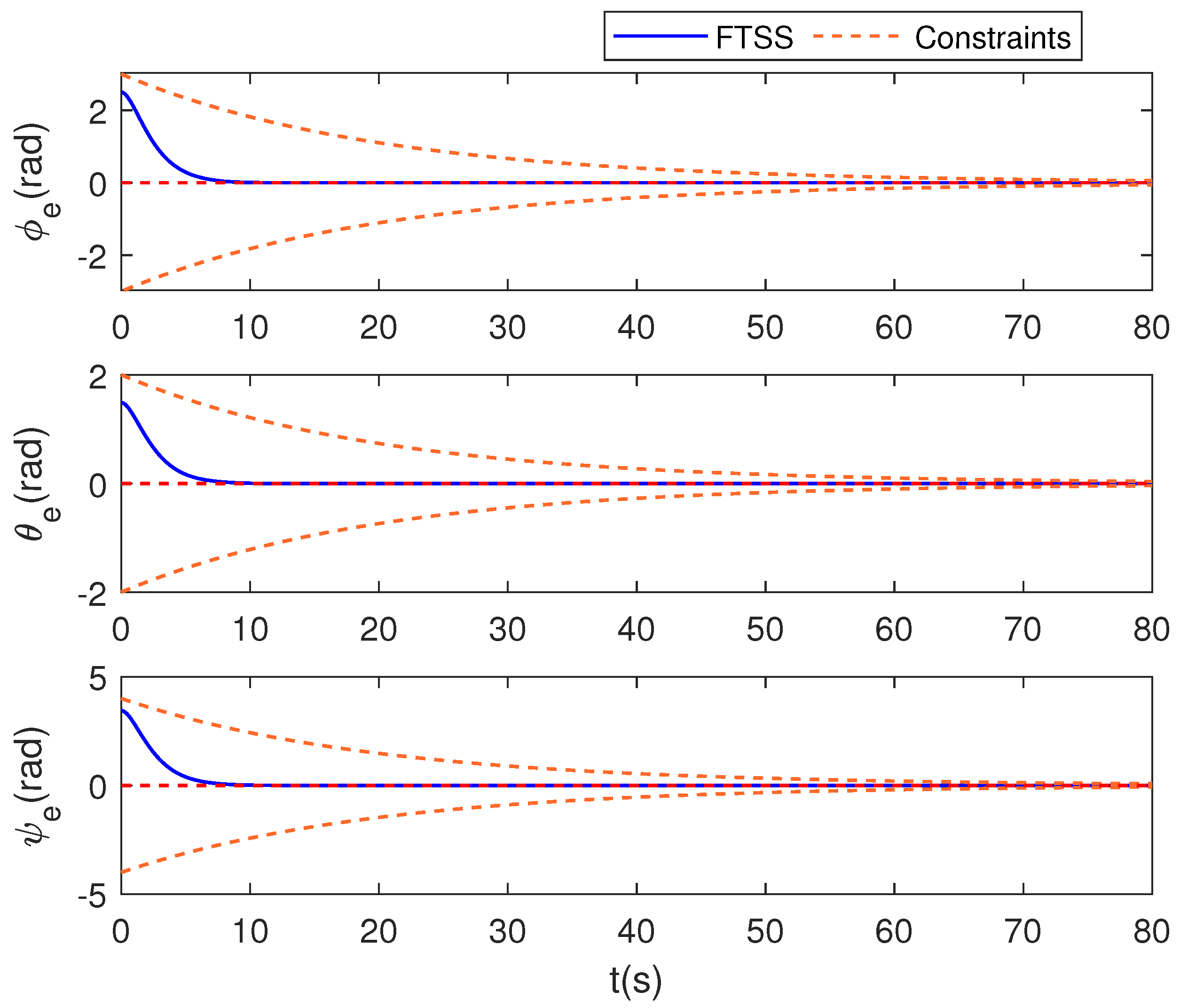
• Furthermore, considering inequality (60), since $V_{1i}\to \infty$ if and only if $\parallel {\mathit{e}}_1\parallel \to {\mathit{\varpi }}_{\left(0\right)}$, and given the initial condition $\parallel {\mathit{e}}_{1\left(0\right)}\parallel \le \parallel {\mathit{\varpi }}_{\left(0\right)}\parallel$, we can rigorously establish that the error constraint ${\mathit{\varpi }}_{\left(t\right)}$ remains strictly satisfied throughout the convergence process.

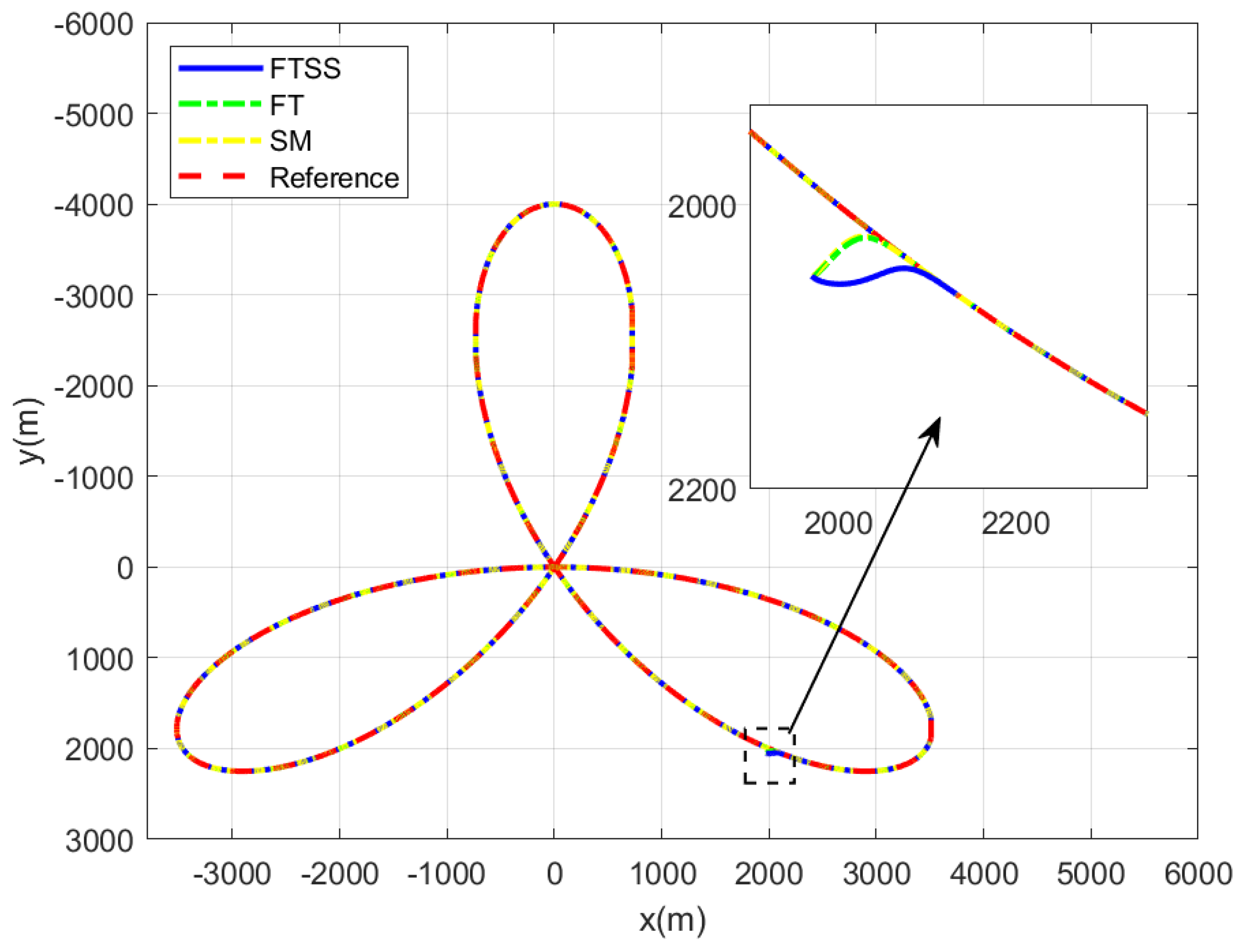
These analytical conclusions finalize the proof. □

Remark 3. 

The control algorithm established in this work can be further applied to other unmanned platforms, such as autonomous underwater vehicles and fixed-wing drones. Remarkably, these unmanned systems operate in environments exhibiting substantial parallels with the operational conditions of unmanned airships addressed in this research, characterized by a low dynamic fluid and persistent external hydrodynamic/aerodynamic disturbances. Furthermore, the inherent strong coupling and pronounced nonlinearity observed in the unmanned airship’s dynamics and control systems bear fundamental similarities to the system characteristics of these unmanned platform vehicles. Through proper modification, the proposed control architecture possesses the potential for effective implementation across related unmanned platforms.

5. Simulation

In this section, a numerical validation of the established tracking control scheme through comprehensive simulation studies are provided. The detailed physical parameters followed the benchmark configuration established in [38], and the reference trajectory of the airship throughout this paper was defined as follows:

$${\mathit{\zeta }}_d\left(t\right)=\left[\begin{array}{c}{x}_d\\ y_d\\ z_d\end{array}\right]={10}^3\times \left[\begin{array}{c}2\times {\mathcal{S}}_{0.005t}+2\times {\mathcal{C}}_{0.0025t}\\ 2\times {\mathcal{S}}_{0.0025t}+2\times {\mathcal{C}}_{0.005t}\\ -19-{10}^{-4}t\end{array}\right]\mathrm{m}$$

(61)

where the desired attitude is denoted as

$${\mathit{\gamma }}_d\left(t\right)=\left[\begin{array}{c}{\varphi }_d\\ {\theta }_d\\ {\psi }_d\end{array}\right]=\left[\begin{array}{c}0\\ arctan2\left({\dot{z}}_d,\sqrt{{\dot{x}}_d^2+{\dot{y}}_d^2}\right)\\ arctan2\left({\dot{y}}_d,{\dot{x}}_d\right)\end{array}\right]\mathrm{rad}.$$

(62)

Remark 4. 

The applied trajectory (three-leaf rose) in (61) demonstrates significant advantages over conventional circular or helical trajectories as a reference tracking trajectory for unmanned airships. Specifically, its sufficient complexity enables the comprehensive validation of airship flight performance under diverse path-following scenarios. The trajectory exhibits complete curvature characteristics, including low-curvature and high-curvature segments with smooth, continuous-curvature transitions. Notably, the trajectory covers an 8 km × 8 km horizontal operational range and a 19 km altitude range in the vertical dimension, matching the actual mission profile of unmanned airships closely.

The initial conditions of the airship were delineated as follows:

$$\begin{array}{cc}\hfill & \mathit{\zeta }={\left[1970,2050,18930\right]}^{\mathrm{T}}\mathrm{m},\mathit{v}={\left[10,0,0\right]}^{\mathrm{T}}\mathrm{m}/\mathrm{s}\hfill \\ \hfill & \mathit{\gamma }={\left[{\displaystyle \frac{\pi }{72}},{\displaystyle \frac{\pi }{90}},{\displaystyle \frac{\pi }{6}}\right]}^{\mathrm{T}}\mathrm{rad},\mathit{\omega }={\left[0,0,0\right]}^{\mathrm{T}}\mathrm{rad}/\mathrm{s}\hfill \end{array}$$

(63)

The constraint boundary parameters for the ETF and external disturbances were defined as follows:

$$\begin{array}{cc}\hfill & {\mathbf{\Omega }}_{0_{\zeta }}={\left[50,75,100\right]}^{\mathrm{T}}\mathrm{m},{\mathbf{\Omega }}_{0_{\gamma }}={\left[3,2,4\right]}^{\mathrm{T}}\mathrm{rad}\hfill \\ \hfill & {\mathbf{\Omega }}_{t_{\zeta }^{\ast }}={\left[5,5,5\right]}^{\mathrm{T}}\mathrm{m},{\mathbf{\Omega }}_{t_{\gamma }^{\ast }}={\left[{\displaystyle \frac{0.1\pi }{180}},{\displaystyle \frac{0.1\pi }{180}},{\displaystyle \frac{0.1\pi }{180}}\right]}^{\mathrm{T}}\mathrm{rad}\hfill \\ \hfill & {\mathit{\lambda }}_{\zeta }={\left[0.05,0.05,0.05\right]}^{\mathrm{T}}\mathrm{m},{\mathit{\lambda }}_{\gamma }={\left[0.05,0.05,0.05\right]}^{\mathrm{T}}\mathrm{rad}\hfill \\ \hfill & \mathit{\delta }=5\times {10}^3\times \left[\begin{array}{c}0.5+2{\mathcal{S}}_{0.1t}\\ 0.4+1.5{\mathcal{C}}_{0.1t}\\ 0.6+1.5{\mathcal{S}}_{0.1t}\\ -2+2{\mathcal{S}}_{0.1t}\\ 1.5+1.5{\mathcal{S}}_{0.1t}\\ 1.5+2{\mathcal{C}}_{0.1t}\end{array}\right]\hfill \end{array}$$

(64)

For the purpose of validating the performance of the presented control strategy, comparisons were executed by adding the following controllers:

• A finite-time controller (denoted as FT controller), whose control law is presented in (65)–(66);

  $${\mathit{\tau }}_{FT}=-{\mathit{MR}}^{-\mathbf{1}}(({\mathit{\hslash }}_{FT1}+{\displaystyle \frac{{\mathit{\hslash }}_{FT1}}{2}}){\mathit{e}}_2+({\mathit{\hslash }}_{FT2}+{\displaystyle \frac{{\mathit{\hslash }}_{FT2}}{2}}){\mathit{ϵ}}_{FT}+\mathfrak{F}\left({\mathit{e}}_1,{\mathit{e}}_2\right)+{\mathit{RM}}^{-\mathbf{1}}\widehat{\mathit{\delta }})$$

  (65)

  $${\mathit{ϵ}}_{FT}={\mathit{e}}_2+({\mathit{\hslash }}_{SM1}+{\displaystyle \frac{{\mathit{\hslash }}_{SM1}}{2}}){\mathit{e}}_1$$

  (66)
• A sliding-mode controller (denoted as SM controller), whose control law is presented in (67)–(68).

  $${\mathit{\tau }}_{SM}=-{\mathit{MR}}^{-\mathbf{1}}(\mathfrak{F}\left({\mathit{e}}_1,{\mathit{e}}_2\right)+{\mathbf{c}}_{\mathit{SM}}{\dot{\mathit{e}}}_1+{\mathit{RM}}^{-\mathbf{1}}\widehat{\mathit{\delta }}+{\mathit{\rho }}_{SM}{\mathit{S}}_{SM}+{\mathbf{k}}_{SM}{\left|{\mathit{S}}_{SM}\right|}^{\mathbf{ð}}\mathrm{sign}\left({\mathit{S}}_{SM}\right))$$

  (67)

  $${\mathit{S}}_{SM}={\dot{\mathit{e}}}_1+{\mathbf{c}}_{SM}{\mathit{e}}_1$$

  (68)

The algorithm parameters of the established control scheme are listed in

Table 1. Algorithm parameters of the control schemes.

FTSS		FT		SM		FTSDO
Parameter	Value	Parameter	Value	Parameter	Value	Parameter	Value
${\alpha }_1$	0.3	${\hslash }_{FT1}$	0.8	$c_{SM}$	0.8	${\alpha }^{\ast }$	2
${\alpha }_2$	0.6	${\hslash }_{FT2}$	0.8	${\rho }_{SM}$	0.4	${\beta }^{\ast }$	2
${\beta }_1$	0.3	${\hslash }_{FT1}$	0.5	$k_{SM}$	2	$p^{\ast }$	0.65
${\beta }_2$	0.6	${\hslash }_{FT2}$	0.5	ð	2	$g^{\ast }$	1.1
$p_1$	0.65	–	–	–	–	$k_1$	0.05
$p_2$	0.65	–	–	–	–	$k_2$	3
$g_1$	1.1	–	–	–	–	–	–
$g_2$	1.1	–	–	–	–	–	–

. Respectively, FTSDO parameters: ${\alpha }^{\ast }$, ${\beta }^{\ast }$, $p^{\ast }$, $g^{\ast }$, $k_1$, $k_2$; proposed FTSS controller parameters: ${\alpha }_1$, ${\alpha }_2$, ${\beta }_1$, ${\beta }_2$, $p_1$, $p_2$, $g_1$, $g_2$; FT controller parameters: ${\mathit{\hslash }}_{FT1},{\mathit{\hslash }}_{FT2},{\mathit{\hslash }}_{FT1},{\mathit{\hslash }}_{FT2}$; and SM controller parameters: ${\mathit{c}}_{\mathit{SM}},{\mathit{\rho }}_{SM},{\mathit{k}}_{SM},\mathbf{ð}$.

A comparative analysis of the experimental results is depicted in Figure 3, Figure 4, Figure 5, Figure 6, Figure 7, Figure 8, Figure 9, Figure 10, Figure 11, Figure 12, Figure 13, Figure 14, Figure 15 and Figure 16. As depicted in Figure 3, all three controllers demonstrated the capability to drive the airship to track a complex spatial curved trajectory. A detailed comparison of the tracking results mapped onto the three planes of an orthogonal Cartesian coordinate system, along with partial enlarged views in Figure 4 and Figure 5, revealed all controllers were capable of rapidly tracking the reference trajectory with high precision.

As evidenced in Figure 6 and Figure 7, the position and attitude tracking errors of the FTSS controller were consistently maintained within the predetermined time-varying bounds during the convergence process, demonstrating its excellent ability to handle time-varying tracking error constraints through the established ETF framework. This validated the established controller’s capability to comply with the mission-required accuracy specifications.

A salient feature observed in Figure 8, Figure 9 and Figure 10 is that the FT controller and SM controller both exhibited significant variability in the convergence times of position and attitude errors. In contrast, the FTSS controller guaranteed the simultaneous fixed-time convergence of these errors. Similarly, as shown in Figure 11 and Figure 12 with the partial enlarged views, a clear inconsistency could be observed in the convergence times of the velocity and angular velocity errors of the FT controller and SM controller. On the other hand, as shown in Figure 13, the FTSS controller was capable of driving all error components towards the neighborhood of the origin synchronously within a fixed-time bound. The comparative results in Figure 8, Figure 9, Figure 10, Figure 11, Figure 12 and Figure 13 conclusively demonstrate the outstanding superiority of the FTSS controller in synchronization convergence performance.

Subsequently, Figure 14 and Figure 15 present the control inputs of these controllers including force inputs in Figure 14 and torque inputs in Figure 15. By combining Figure 8, Figure 9, Figure 10, Figure 11, Figure 12, Figure 13, Figure 14 and Figure 15, it can be concluded that the convergence time of the controller was negatively correlated with the magnitude of the system input, which means a larger input fluctuation was often accompanied by a faster convergence speed. Additionally, after the system reached stability, the input of these controller curves largely coincided, indicating that the control inputs were primarily focused on counteracting environmental disturbances.

Finally, Figure 16 presents the estimation errors obtained by the FTSDO. It is evident that all components of the estimation errors approached the vicinity of zero simultaneously and promptly, demonstrating that the FTSDO accurately estimated unknown disturbances with guaranteed synchronized convergence properties.

6. Conclusions

This work discussed the synchronized trajectory tracking in fixed time of unmanned airships considering error constraints and unknown perturbations. An FTSDO was developed to achieve precise disturbance estimation, featuring simultaneous convergence of all estimation error components to zero in fixed time. An innovative ETF was applied to strictly enforce tracking error constraints within prescribed bounds during the convergence process. To achieve synchronous fixed-time convergence in both trajectory tracking and disturbance estimation, the NNS function was integrated into the FTSS controller and FTSDO framework. A rigorous mathematical analysis demonstrated the proposed control scheme’s synchronized fixed-time stability, with numerical simulations confirming its advanced control performance. In future research endeavors, the primary focus will be on the development of full-state constrained controllers for unmanned airships using a partially synchronized control scheme, which will ensure prioritized convergence of attitude errors, followed by precise position tracking.

References

1. Durán-Delfín, J.; García-Beltrán, C.D.; Guerrero-Sánchez, M.E.; Valencia-Palomo, G.; Hernández-González, O. Modeling and Passivity-Based Control for a convertible fixed-wing VTOL. Appl. Math. Comput. 2024, 461, 128298. [Google Scholar] [CrossRef]
2. Zheng, B.; Zhu, M.; Guo, X.; Ou, J.; Yuan, J. Path planning of stratospheric airship in dynamic wind field based on deep reinforcement learning. Aerosp. Sci. Technol. 2024, 150, 109173. [Google Scholar] [CrossRef]
3. Sun, R.; Ahn, C.K.; Liu, D.; Wang, W.; Zhang, C. Near-asteroid spacecraft formation control with prescribed-performance: A dynamic event-triggered reinforcement learning control approach. Aerosp. Sci. Technol. 2025, 161, 110138. [Google Scholar] [CrossRef]
4. Ye, Z.; Cai, G.; Xu, H.; Shang, Y.; Hu, C. Prescribed Performance Sliding Mode Fault-Tolerant Tracking Control for Unmanned Morphing Flight Vehicles with Actuator Faults. Drones 2025, 9, 292. [Google Scholar] [CrossRef]
5. Mechali, O.; Xu, L. Distributed fixed-time sliding mode control of time-delayed quadrotors aircraft for cooperative aerial payload transportation: Theory and practice. Adv. Space Res. 2023, 71, 3897–3916. [Google Scholar] [CrossRef]
6. Airaldi, F.; De Schutter, B.; Dabiri, A. Reinforcement Learning with Model Predictive Control for Highway Ramp Metering. IEEE Trans. Intell. Transp. Syst. 2025, 26, 5988–6004. [Google Scholar] [CrossRef]
7. Taheri, S.; Amiri, A.J.; Razban, A. Real-world implementation of a cloud-based MPC for HVAC control in educational buildings. Energy Convers. Manag. 2024, 305, 118270. [Google Scholar] [CrossRef]
8. Li, Y.; Tong, S. Adaptive backstepping control for uncertain nonlinear strict-feedback systems with full state triggering. Automatica 2024, 163, 111574. [Google Scholar] [CrossRef]
9. Li, Y.; Fan, Y.; Li, K.; Liu, W.; Tong, S. Adaptive optimized backstepping control-based RL algorithm for stochastic nonlinear systems with state constraints and its application. IEEE Trans. Cybern. 2021, 52, 10542–10555. [Google Scholar] [CrossRef]
10. Montoya-Morales, J.; Guerrero-Sánchez, M.; Valencia-Palomo, G.; Hernández-González, O.; López-Estrada, F.; Hoyo-Montaño, J. Real-time robust tracking control for a quadrotor using monocular vision. Proc. Inst. Mech. Eng. Part G J. Aerosp. Eng. 2023, 237, 2729–2741. [Google Scholar] [CrossRef]
11. Wang, Y.; Zong, G.; Yang, D.; Shi, K. Finite-time adaptive tracking control for a class of nonstrict feedback nonlinear systems with full state constraints. Int. J. Robust Nonlinear Control 2022, 32, 2551–2569. [Google Scholar] [CrossRef]
12. Zhou, B.; Michiels, W.; Chen, J. Fixed-time stabilization of linear delay systems by smooth periodic delayed feedback. IEEE Trans. Autom. Control 2021, 67, 557–573. [Google Scholar] [CrossRef]
13. Yu, L.; He, G.; Wang, X.; Zhao, S. Robust fixed-time sliding mode attitude control of tilt trirotor UAV in helicopter mode. IEEE Trans. Ind. Electron. 2021, 69, 10322–10332. [Google Scholar] [CrossRef]
14. Zhang, Y.; Zhu, M.; Chen, T.; Zheng, Z. Distributed event-triggered fixed-time formation and trajectory tracking control for multiple stratospheric airships. ISA Trans. 2022, 130, 63–78. [Google Scholar] [CrossRef]
15. Xie, X.; Sheng, T.; Chen, X. Dynamic event-triggered and self-triggered fault-tolerant attitude control for multiple spacecraft systems with uncertainties and input saturation. IEEE Trans. Aerosp. Electron. Syst. 2024, 60, 2922–2933. [Google Scholar] [CrossRef]
16. Sun, H.; Zong, G.; Cui, J.; Shi, K. Fixed-time sliding mode output feedback tracking control for autonomous underwater vehicle with prescribed performance constraint. Ocean Eng. 2022, 247, 110673. [Google Scholar] [CrossRef]
17. Song, X.; Sun, P.; Song, S.; Stojanovic, V. Event-driven NN adaptive fixed-time control for nonlinear systems with guaranteed performance. J. Frankl. Inst. 2022, 359, 4138–4159. [Google Scholar] [CrossRef]
18. Li, X.; Qin, H.; Li, L.; Xue, Y. Adaptive fixed-time fuzzy formation control for multiple AUV systems considering time-varying tracking error constraints and asymmetric actuator saturation. Ocean. Eng. 2024, 297, 116936. [Google Scholar] [CrossRef]
19. Hu, X.; Wei, X.; Gong, Q.; Gu, J. Adaptive synchronization of marine surface ships using disturbance rejection without leader velocity. ISA Trans. 2021, 114, 72–81. [Google Scholar] [CrossRef]
20. Gao, Y.; Li, D.; Ge, S.S. Time-synchronized tracking control for 6-DOF spacecraft in rendezvous and docking. IEEE Trans. Aerosp. Electron. Syst. 2021, 58, 1676–1691. [Google Scholar] [CrossRef]
21. Zhai, A.; Wang, J.; Zhang, H.; Lu, G.; Li, H. Adaptive robust synchronized control for cooperative robotic manipulators with uncertain base coordinate system. ISA Trans. 2022, 126, 134–143. [Google Scholar] [CrossRef] [PubMed]
22. Li, D.; Ge, S.S.; Lee, T.H. Time-Synchronized Control: Analysis and Design; Springer: New York, NY, USA, 2022. [Google Scholar]
23. Jang, S.G.; Yoo, S.J. Predefined-time-synchronized backstepping control of strict-feedback nonlinear systems. Int. J. Robust Nonlinear Control 2023, 33, 7563–7582. [Google Scholar] [CrossRef]
24. Wang, D.; Ge, S.S.; Liang, X.; Li, D. Time-synchronized formation control of unmanned surface vehicles. IEEE Trans. Intell. Veh. 2024. early access. [Google Scholar] [CrossRef]
25. Guan, H.; Sui, S.; Sui, Y.; Chen, C.P. NN-based adaptive event-triggered predefined time control of flexible joint robot with full-state error constraints. Neurocomputing 2025, 631, 129658. [Google Scholar] [CrossRef]
26. Pan, Y.; Chen, Y.; Liang, H. Event-triggered predefined-time control for full-state constrained nonlinear systems: A novel command filtering error compensation method. Sci. China Technol. Sci. 2024, 67, 2867–2880. [Google Scholar] [CrossRef]
27. Ding, Z.; Wang, H.; Sun, Y.; Qin, H. Adaptive prescribed performance second-order sliding mode tracking control of autonomous underwater vehicle using neural network-based disturbance observer. Ocean Eng. 2022, 260, 111939. [Google Scholar] [CrossRef]
28. Wang, Y.; Zong, G.; Zhao, X.; Yi, Y. Adaptive practical fixed-time synchronized tracking control of ASV with prescribed performance. Automatica 2024, 166, 111716. [Google Scholar] [CrossRef]
29. Zhang, L.; Wang, P.; Qian, C.; Hua, C. Adaptive Trajectory Tracking Error Constraint Control of Unmanned Underwater Vehicle Based on a Fully Actuated System Approach. J. Syst. Sci. Complex. 2024, 37, 2633–2653. [Google Scholar] [CrossRef]
30. He, H.; Wang, N.; Huang, D.; Han, B. Active vision-based finite-time trajectory-tracking control of an unmanned surface vehicle without direct position measurements. IEEE Trans. Intell. Transp. Syst. 2024, 25, 12151–12162. [Google Scholar] [CrossRef]
31. Huang, Y.; Zhu, M.; Zheng, Z.; Feroskhan, M. Fixed-time autonomous shipboard landing control of a helicopter with external disturbances. Aerosp. Sci. Technol. 2019, 84, 18–30. [Google Scholar] [CrossRef]
32. Sun, L.; Sun, K.; Guo, X.; Yuan, J.; Zhu, M. Prescribed-time error-constrained moving path following control for a stratospheric airship with disturbances. Acta Astronaut. 2023, 212, 307–315. [Google Scholar] [CrossRef]
33. Hernández-González, O.; Targui, B.; Valencia-Palomo, G.; Guerrero-Sánchez, M.E. Robust cascade observer for a disturbance unmanned aerial vehicle carrying a load under multiple time-varying delays and uncertainties. Int. J. Syst. Sci. 2024, 55, 1056–1072. [Google Scholar] [CrossRef]
34. An, S.; Wang, L.; He, Y. Robust fixed-time tracking control for underactuated AUVs based on fixed-time disturbance observer. Ocean Eng. 2022, 266, 112567. [Google Scholar] [CrossRef]
35. Polyakov, A. Nonlinear feedback design for fixed-time stabilization of linear control systems. IEEE Trans. Autom. Control 2011, 57, 2106–2110. [Google Scholar] [CrossRef]
36. Li, D.; Ge, S.S.; Lee, T.H. Fixed-time-synchronized consensus control of multiagent systems. IEEE Trans. Control. Netw. Syst. 2020, 8, 89–98. [Google Scholar] [CrossRef]
37. Li, D.; Yu, H.; Tee, K.P.; Wu, Y.; Ge, S.S.; Lee, T.H. On time-synchronized stability and control. IEEE Trans. Syst. Man, Cybern. Syst. 2021, 52, 2450–2463. [Google Scholar] [CrossRef]
38. Luo, X.; Zhu, M.; Zhang, Y.; Zheng, Z.; Chen, T. Self-triggered fuzzy trajectory tracking control for the stratospheric airship. Adv. Space Res. 2024, 74, 5874–5889. [Google Scholar] [CrossRef]
Figure 1. The structure and coordinate system of the unmanned airship.
Drones 09 00403 g001
Figure 2. Architecture of the control scheme of the unmanned airship.
Drones 09 00403 g002
Figure 3. Three–dimensional trajectory tracking performance of the airship.
Drones 09 00403 g003
Figure 4. x–y plane trajectory tracking performance of the airship.
Drones 09 00403 g004
Figure 5. x–z and y–z plane trajectory tracking performance of the airship.
Drones 09 00403 g005
Figure 6. Position tracking errors of the FTSS controller.
Drones 09 00403 g006
Figure 7. Attitude tracking errors of the FTSS controller.
Drones 09 00403 g007
Figure 8. Position and attitude tracking errors of the FT controller.
Drones 09 00403 g008
Figure 9. Position and attitude tracking errors of the SM controller.
Drones 09 00403 g009
Figure 10. Position and attitude tracking errors of the FTSS controller.
Drones 09 00403 g010
Figure 11. Linear velocity and angular velocity errors of the FT controller.
Drones 09 00403 g011
Figure 12. Linear velocity and angular velocity errors of the SM controller.
Drones 09 00403 g012
Figure 13. Linear velocity and angular velocity errors of the FTSS controller.
Drones 09 00403 g013
Figure 14. Force input of the airship.
Drones 09 00403 g014
Figure 15. Torque input of the airship.
Drones 09 00403 g015
Figure 16. Disturbance estimation errors of the FTSDO.
Drones 09 00403 g016