A Robust Aerodynamic Design Optimization Methodology for UAV Airfoils Based on Stochastic Surrogate Model and PPO-Clip Algorithm

Abstract

Unmanned Aerial Vehicles (UAVs) are widely used in meteorology and logistics due to their unique advantages nowadays. During their lifecycle, uncertainties—such as flight condition variations—can significantly affect both design and performance, making Robust Aerodynamic Design Optimization (RADO) essential. However, existing RADO methodologies face high computational cost of uncertainty analysis and inefficiency of conventional optimization algorithms. To address these challenges, this paper proposed a novel RADO methodology integrating a Stochastic Kriging (SK) surrogate model with the PPO-Clip reinforcement learning algorithm, targeting atmospheric uncertainties encountered by turbojet-powered UAVs in transonic cruise. The SK surrogate model, constructed via Maximin Latin Hypercube Sampling and refined using the Expected Improvement infill criterion, enabled efficient uncertainty quantification. Based on the trained surrogate model, a PPO-Clip-based RADO framework with tailored reward and state transition functions was established. Applied to the RAE2822 airfoil under Mach number perturbations, the methodology demonstrated superior reliability and efficiency compared with L-BFGS-B and PSO algorithms.

1. Introduction

With the rapid advancement of technology, Unmanned Aerial Vehicles (UAVs) are emerging as a transformative force across a wide range of fields, owing to their unique advantages and broad application prospects. They have been widely employed in areas such as meteorological research, disaster early warning, geospatial mapping, and logistics delivery. In the entire lifecycle of an UAV—from design and manufacturing through operation—uncertainty is an objective and unavoidable factor. Examples include variations in structural properties due to the material’s physicochemical characteristics and assembly tolerances; deviations in exterior geometry arising during fabrication, use, or maintenance; changes in takeoff weight, flight altitude, and airspeed during operation; and disturbances in atmospheric parameters such as air density, humidity, and wind speed during flight [1]. These uncertainty factors make the performance of the designed UAV highly sensitive, potentially leading to severe degradation or even failure, which can result in increased economic costs and mission failure [2]. If such uncertainties are taken into account and quantitatively assessed during the UAV design phase, their negative impact can be significantly reduced. Design methodologies that explicitly account for uncertainty are commonly called robust design. Robust design seeks to render performance objectives insensitive to small fluctuations in design variables—i.e., to ensure system stability under stochastic influences [3]. First introduced by Taguchi et al. [4], robust design theory rapidly gained widespread acceptance in industry and academia due to its significant practical engineering value. Building on Taguchi’s foundation, robust design methodologies evolved systematically and were extended to aerodynamic optimization in the UAV domain [5]. Robust Aerodynamic Design Optimization (RADO) has thus become a core technology for addressing the multi-source uncertainties inherent in UAV design [6,7,8,9].

Within RADO, two key areas are uncertainty analysis and optimization algorithms. Reliable uncertainty analysis underpins RADO: only rapid and accurate uncertainty analysis can furnish the data necessary to support the design optimization. An effective optimization algorithm lies at the heart of RADO, interlinking all modules of the process and governing the initiation, execution, and termination of the optimization process.

The essence of uncertainty analysis lies in Uncertainty Quantification (UQ), which provides quantitative estimates of how input uncertainties affect system outputs [10]. The central challenge is characterizing solutions when deterministic parameters are modeled as random variables—specifically, computing objective function’s mean and variance—along with other statistical information, such as its probability density function. Advances in computer hardware and numerical methods have made Computational Fluid Dynamics (CFD) a mature tool for RADO, offering lower design cost, shorter computational turnaround, and greater versatility than traditional experiments. However, when quantifying uncertainty in a UAV’s aerodynamic performance, each design point must be evaluated under multiple operating conditions, which demands substantial computational resources and leads to very low efficiency. To address this, surrogate-modeling techniques have become prevalent in UAV aerodynamic optimization to supplant time-consuming numerical simulations, enabling rapid estimation of lift and drag coefficients and pressure distributions. Building on this concept, computationally inexpensive surrogate models can likewise be used during UQ in lieu of expensive CFD analyses, thereby markedly improving efficiency. Now surrogate-based UQ methods fall into two categories: Deterministic Metamodel-Based Approaches (DMBA) and Stochastic Metamodel-Based Approaches (SMBA). DMBA requires separate estimation of the mean and variance at each design point, leading to significant computational overhead; moreover, deterministic surrogate models are not inherently tailored to uncertainty modeling and may fail to capture complex stochastic behavior. In contrast, SMBA offers lower computational cost, targeted treatment of uncertainty, and more reliable statistical responses [11]. Common stochastic surrogate frameworks include Polynomial Chaos (PC) [12,13], Stochastic Radial Basis Functions (Stochastic RBF) [14] surrogate model, and Stochastic Kriging (SK) [3,15,16] surrogate model. The SK surrogate model, as an extension of classical Kriging surrogate model into the stochastic domain, not only retains deterministic Kriging surrogate model’s inherent advantage of addressing spatially uniform uncertainty via the so-called “nugget effect,” but also incorporates both intrinsic and extrinsic uncertainties directly into the model’s Mean Square Error (MSE) formulation, yielding reliable predictions of a system’s mean and variance under uncertainty. This approach has already been applied to RADO of aircraft surfaces [3,17]. Consequently, SK surrogate model offers strong performance and promising prospects for the RADO of UAVs.

Conventional optimization algorithms fall into gradient-based and heuristic categories. Although gradient-based optimization algorithms, such as Stochastic Gradient Descent (SGD) [18] and Limited-memory Broyden–Fletcher–Goldfarb–Shanno with Bound constraints (L-BFGS-B) [19], exhibit efficiency that is largely independent of the number of design variables, they are prone to becoming trapped in local optima [20]. Heuristic algorithms—such as Genetic Algorithms (GA) [21] and Particle Swarm Optimization (PSO) [22]—are relatively easy to implement and offer strong global search capability, but they suffer from a relatively slow convergence rate and limited scalability with respect to the number of design variables, leading to reduced computational efficiency in high-dimensional design spaces [23]. Both classes of algorithms have inherent trade-offs. With the rapid development of Artificial Intelligence (AI), AI-powered optimization algorithms are emerging as promising tools for efficient RADO of UAVs. Among them, Reinforcement Learning (RL) algorithms are gaining increasing traction in UAV design applications. RL operates through continuous interaction between an agent and its environment, where the environment provides state and reward signals, and the agent iteratively refines its policy based on this feedback—learning progressively until it converges to an optimal strategy for handling the environment [24]. Well-known RL methods include Q-learning [25], State-Action-Reward-State-Action (SARSA) [26], Deep Deterministic Policy Gradient (DDPG) [27], Trust Region Policy Optimization (TRPO) [28], Asynchronous Advantage Actor-Critic (A3C) [29], and Proximal Policy Optimization (PPO) [30]. Currently, RL has been primarily applied to control and decision-making tasks in UAV design, such as intelligent air combat [31,32], attitude control [33,34], trajectory planning [35,36], and autonomous obstacle avoidance [37,38]. Among RL algorithms, Proximal Policy Optimization with Clipped Surrogate Objective (PPO-Clip) is a widely used variant of the PPO algorithm. By constraining the magnitude of policy updates, it ensures training stability, making it the most prevalent form of PPO. Due to its strong convergence properties, high stability and computational efficiency, PPO-Clip is particularly well-suited for RADO of UAVs.

As the foundational element of an aircraft’s aerodynamic performance, the airfoil—owing to its simple structure and low-dimensional parametric representation—is frequently chosen as the example in studies on RADO. In recent years, extensive research has been conducted on both UQ techniques and optimization algorithms for robust airfoil design. In terms of UQ, DMBA have evolved from Kriging surrogate model to multi-fidelity surrogate model [39]. Meanwhile, SMBA has progressed from Non-Intrusive Polynomial Chaos (NIPC) [40] to uncertainty-aware deep learning surrogate models [41]. On the optimization algorithms, the field has advanced from traditional multi-objective algorithms to gradient-based approaches. The following are representative studies in recent years on RADO of airfoils: Liu et al. (2022) addressed the RADO of a transonic airfoil under Mach number uncertainty by proposing a novel framework that combined NIPC for UQ, Kriging surrogate modeling, a Lower Confidence Bound (LCB) infill criterion, and the GlobalSearch optimization algorithm. This integrated strategy significantly enhanced aerodynamic robustness—particularly through drag reduction—while reducing the computational cost to just 20.76% of that incurred by conventional deterministic methods [42]. Jofre et al. (2022) proposed an SGD framework incorporating an AdaGrad-style adaptive gradient method, explicitly formulated to manage both aleatoric and epistemic uncertainties in aerodynamic airfoil design. By using a small number of random samples per iteration to estimate both the performance metric and its gradient—and embedding both mean and variance into the optimization objective—they performed robust optimization of the NACA 0012 airfoil across different Reynolds numbers and RANS turbulence models. The computational cost was only a modest factor higher than that of a single-point deterministic design, yet the method substantially reduced uncertainty, achieving more robust aerodynamic performance [43]. Chen et al. (2024) proposed a data-driven framework based on Distributionally Robust Optimization (DRO) to address aerodynamic shape design under uncertainty in flight conditions. The framework constructs ambiguity sets via $\varphi$ divergence to quantify distributional shifts. By theoretically linking DRO with Taguchi methods, it enhanced design robustness. A constrained optimization problem was solved using a stochastic gradient algorithm. In transonic turbulent-flow airfoil design experiments, the method delivered promising preliminary results, improving robustness against distributional shifts [44]. Sharpe et al. (2025) developed NeuralFoil, a hybrid physics-informed machine learning framework designed to address the convergence failures and non-smooth behavior that hinder traditional RADO tools such as XFoil. It introduces a novel surrogate model UQ technique (termed analysis confidence) embedded within a physics-constrained neural architecture. Leveraging its $C^{\infty }$ continuity and compatibility with automatic differentiation, NeuralFoil enables gradient-based optimization. Quantitatively, when matching XFoil-level accuracy, it achieves 8–30× speedups for single-point analyses and up to 1000× acceleration in batched, multipoint evaluations, all while maintaining mean drag prediction errors as low as 0.37%. Within seconds, it can generate optimized airfoils that closely resemble expert-designed configurations, thus substantially enhancing the robustness and efficiency of aerodynamic design workflows [45]. Previous studies have provided a solid foundation for the further development of RADO methodologies for airfoils and have inspired the research direction of this paper.

To overcome the key challenges of high computational cost in UQ and the inefficiency of conventional optimization algorithms in achieving rapid optimization in the current RADO methodologies of UAVs, this paper proposed a new methodology that combines a trained SK surrogate model for rapid and accurate UQ of UAV’s aerodynamic performance with the PPO-Clip algorithm for efficient RADO. Using the commonly employed RAE2822 airfoil for UAVs under Mach number perturbations as a case study, the effectiveness of the proposed methodology was validated through analysis of the optimization results.

The rest of the paper is organized as follows. Section 2 presents the RADO process for UAV airfoils, including the determination of optimization objectives and constraints, the parameterization method for the airfoil, and an overview of the parameter optimization. Section 3 introduces the SK surrogate model used in parameter optimization. A SK surrogate model meeting the required accuracy was trained using Maximin Latin Hypercube Sampling (MM-LHS) combined with the Expected Improvement (EI) infill criterion. Section 4 describes the PPO-Clip algorithm applied in the parameter optimization, detailing the design of the reward and state functions tailored to the RADO objectives and constraints, as well as structural modifications made to the algorithm to enhance its stability and reliability. Section 5 applies the trained SK surrogate model and the modified PPO-Clip algorithm to perform RADO of the RAE2822 airfoil under Mach number perturbations. The optimization results were analyzed and compared with those obtained using L-BFGS-B and PSO algorithms, thereby validating the reliability and efficiency of the proposed RADO methodology. Section 6 presents the conclusions and future outlook.

2. Robust Aerodynamic Design Optimization Process for UAV Airfoils

The RADO process for UAV airfoils is illustrated in Figure 1. It primarily consists of three components: determination of optimization objectives and constraints, airfoil parameterization, and parameter optimization. First, the optimization objectives and constraints are determined based on the RADO problem. Next, the airfoil geometry is parameterized to enable quantitative optimization. Finally, parameter optimization is performed, wherein robust aerodynamic analysis and constraint evaluation yield an integrated optimization objective value integrating both optimization objectives and constraints. This value is iteratively optimized using the PPO-Clip algorithm to identify the optimized airfoil parameters. This section provides a description of each component.

2.1. Determination of Optimization Objectives and Constraints

This paper addresses the issue of atmospheric uncertainties encountered by turbojet-powered UAVs during transonic cruise flights. To minimize the impact of Mach number variations on aerodynamic drag and to enhance cruise efficiency and endurance, an RADO of the UAV airfoil was conducted.

The RADO problem of the UAV airfoil can be formulated as:

$$\begin{array}{l}Min:\hspace{1em}\hspace{1em}z[{\mu }_{cd},{\sigma }_{cd}^2]\\ \hspace{1em}\hspace{1em}\hspace{1em}\hspace{1em}Ma~\mathcal{U}(0.71, 0.75)\\ S.T.\hspace{1em}\hspace{1em} C_l(s,Ma)=0.68\\ \hspace{1em}\hspace{1em}\hspace{1em}\hspace{1em}{\overline{c}}_{max}\ge 0.12\\ \hspace{1em}\hspace{1em}\hspace{1em}\hspace{1em}{\sigma }_{cd}^2\ge 5\times {10}^{-7}\\ \hspace{1em}\hspace{1em}\hspace{1em}\hspace{1em}s\in [-0.2,0.2]\\ Variable: s\end{array}$$

(1)

The RADO problem of the UAV airfoil considers Mach number as an uncertain factor in the flight conditions. The perturbation interval of the Mach number is set to 0.71 to 0.75, reflecting the typical range encountered during high-altitude, long-endurance cruise missions. Here, $Ma~\mathcal{U}(0.71, 0.75)$ represents the assumption that the Mach number is uniformly distributed in the interval [0.71, 0.75]. The objective of optimization is to minimize both the mean of the drag coefficient ${\mu }_{cd}$ and the variance of the drag coefficient ${\sigma }_{cd}^2$. Reducing the mean of the drag coefficient improves the cruise efficiency and endurance of the UAV, while reducing the variance enhances the stability of flight performance under varying atmospheric conditions. This constitutes a multi-objective optimization problem, and $z[{\mu }_{cd},{\sigma }_{cd}^2]$ refers to the use of either the weighted sum approach or by establishing a multi-objective optimization mode to address it. There are four constraints:

• Constant Lift Coefficient Limit: $C_l(s,Ma)=0.68$ indicates that the lift coefficient of the UAV airfoil is fixed at 0.68. Based on this constraint, RADO is carried out for the UAV airfoil.
• Airfoil Thickness Limit: the maximum thickness of the airfoil ${\overline{c}}_{max}$ must be no less than 0.12 to ensure adequate aero-structural strength and safety margins under the UAV’s lightweight structural design.
• Drag Coefficient Variance Limit: the variance of the drag coefficient ${\sigma }_{cd}^2$ should be no less than $5\times {10}^{-7}$ to prevent numerical instability during the computation process caused by excessively small variance.
• Airfoil Parameter Variation Range Limit: the variation range of the airfoil parameters (i.e., airfoil parameter adjustments) $s$ is restricted to $[-0.2,0.2]$ in order to control the extent of optimization. This prevents excessive parameter changes that could hinder convergence or lead to unpredictable aerodynamic characteristics and manufacturing challenges for the UAV airfoil.

Since this paper focused on optimizing the RAE2822 airfoil, the description of the new airfoil was based on the approach of “baseline airfoil parameters + airfoil parameter adjustments,” i.e., new airfoil parameters = RAE2822 baseline airfoil parameters + airfoil parameter adjustments. The airfoil parameter adjustments $s$ serve as the design variables in the optimization process.

2.2. Airfoil Parameterization

To accurately characterize the UAV airfoil geometry using a limited number of variables, this paper employed the Class-Shape Transformation (CST) parameterization method [46,47] which features a small set of control parameters with clear geometric interpretations and strong modeling capability [48]. In this paper, the airfoil geometry was described using 9 design variables, each corresponding to the weight coefficient of a Bernstein polynomial. Specifically, the upper surface of the airfoil is represented by a third-order Bernstein polynomial with 4 variables, while the lower surface is described by a fourth-order polynomial with 5 variables. As an illustrative example,

Table 1. Influence of parametric variables on the geometric shape of the RAE2822 airfoil.

Variable No.	Value	Surface	Controlled Region	Geometric Influence
1	1.259521	Upper	Near leading edge	Controls leading-edge thickness or camber
2	1.518066	Upper	Forward-mid section	Controls mid-fore thickness or camber
3	2.076904	Upper	Aft-mid section	Controls mid-aft thickness or camber
4	1.946289	Upper	Near trailing edge	Controls upper-surface thickness near trailing edge
5	−1.179688	Lower	Near leading edge	Controls leading-edge thickness or camber
6	−1.671875	Lower	Forward-mid section	Controls mid-fore thickness or camber
7	−1.757813	Lower	Aft-mid section	Controls mid-aft thickness or camber
8	−1.210938	Lower	Near trailing edge	Controls lower-surface thickness near trailing edge
9	0.601563	Lower	Trailing edge	Slightly adjusts the trailing-edge camber

presents the parameterization of the RAE2822 airfoil, demonstrating how each of the 9 variables influences specific geometric features.

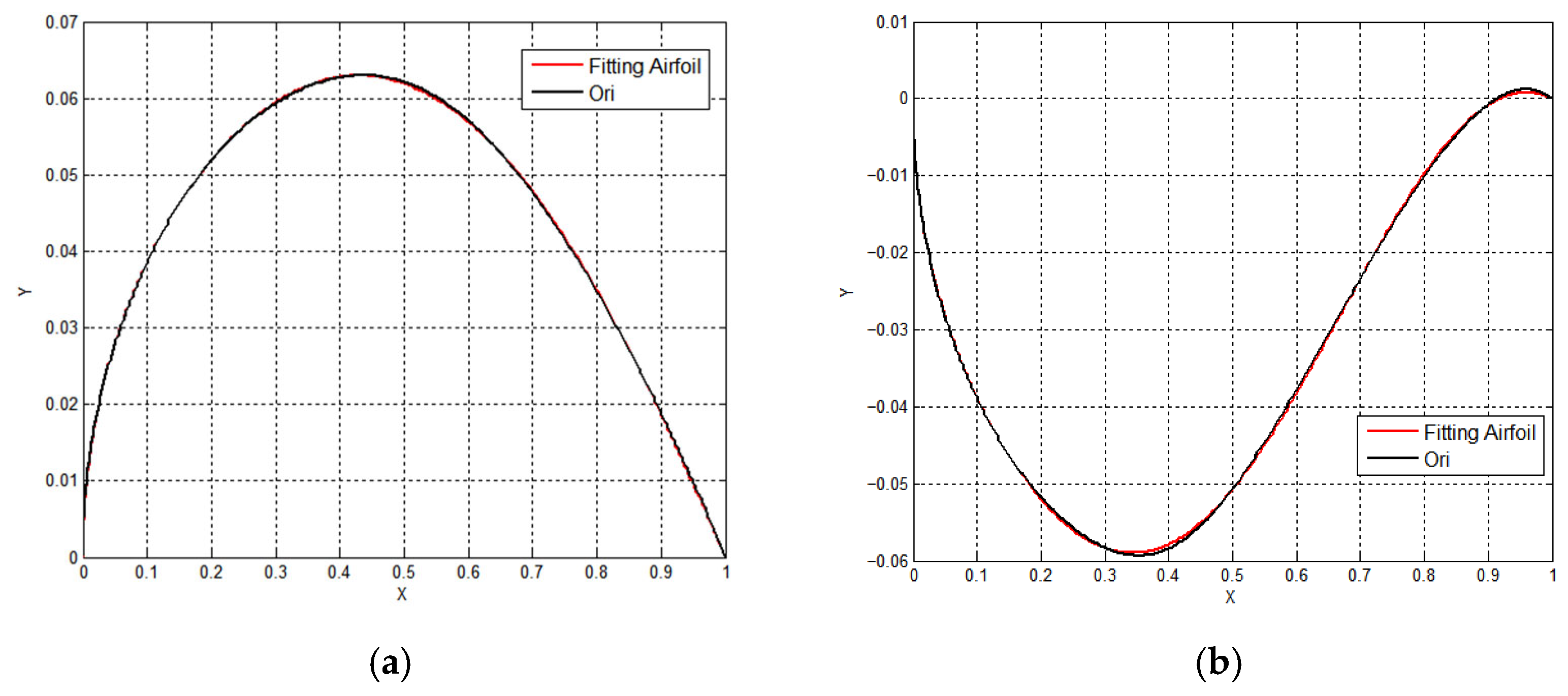
The CST parameterization method is implemented as part of an in-house code, and its effectiveness was validated in Figure 2.

The RAE2822 airfoil was selected as the test case. Figure 2a,b showed the upper and lower surfaces of the airfoil before and after CST parameterization, respectively. As observed, this method could effectively approximate the target airfoil. It also showed that the UAV airfoil could be described with considerable accuracy using fewer variables, which is highly beneficial for UAV design optimization within limited computational resources.

2.3. Overview of Parameter Optimization

The core of the parameter optimization module lies in leveraging the SK surrogate model and the PPO-Clip algorithm to efficiently identify UAV airfoil designs with strong robustness to Mach number perturbations, while satisfying engineering constraints.

The parameter optimization module is composed of robust aerodynamic analysis, constraint evaluation, integrated optimization objective calculation, and the PPO-Clip algorithm optimization. The integrated optimization objective consists of two optimization objectives (minimizing the mean and variance of the drag coefficient) and three constraints (airfoil thickness limit, drag coefficient variance limit, and airfoil parameter variation range limit). The constant lift coefficient limit is directly enforced by the CFD solver, which will be introduced in Section 3, through dynamic adjustment of the cruise angle of attack. Therefore, it does not need to be explicitly included in the computation of the integrated optimization objective or in the subsequent training of the SK surrogate model. Parameter optimization aims to find the airfoil parameter adjustments and updated airfoil parameters that minimize the integrated optimization objective.

For the two optimization objectives, the SK surrogate model is used to compute the mean and variance of the drag coefficient for robust aerodynamic analysis. A weighted-sum approach is applied by assigning different weights to the mean and variance terms of the drag coefficient, thereby transforming the multi-objective optimization problem into a single-objective one. For the three constraints, the designed ThicknessCheck function, VarianceCheck function, soft_clip function, and BoundaryCheck function are used for constraint evaluation. Specifically, the airfoil thickness limit and drag coefficient variance limit are handled by applying penalty terms to individuals that exceed the limits, with the ThicknessCheck function and VarianceCheck function used to obtain the thickness penalty term and variance penalty term, respectively. The airfoil parameter variation range limit is managed using the soft_clip function for soft clipping, and the BoundaryCheck function is used to obtain boundary penalty term to reduce boundary accumulation.

The PPO-Clip algorithm interacts continuously with the environment using the above information to train the optimal policy and obtain the optimized airfoil parameter adjustments and optimized airfoil parameters that meet the integrated optimization objective. The SK surrogate model is employed to rapidly estimate the mean and variance of the drag coefficient, which facilitates the training of the optimal policy represented by a neural network. The detailed parameter optimization process, including the definitions of the ThicknessCheck function, VariancePenalty function, soft_clip function and BoundaryPenalty function will be introduced in Section 4.

3. Construction and Training of the Stochastic Kriging Surrogate Model

Traditional CFD-based UQ is computationally expensive and cannot meet the demand for evaluating large numbers of samples required in the RADO of UAVs. The SK surrogate model, as an efficient stochastic modeling approach, significantly reduces the computational burden associated with evaluating UAV airfoil performance under uncertain flight conditions. In the RADO process for UAV airfoils, the SK surrogate model was employed to quantify the optimization objectives (i.e., the mean and variance of the drag coefficient) for robust aerodynamic analysis. Therefore, constructing and training an accurate SK surrogate model is crucial. This section first provides a brief overview of the construction method for the SK surrogate model, followed by a detailed description of its training process. The training involved sampling using the MM-LHS, assessing the fitting accuracy of the SK model using an error function, and refining the model through the EI infill criterion. Finally, the accuracy of the mean and variance predictions of the drag coefficient from the SK surrogate model was validated using the mean relative error and mean logarithmic error.

3.1. The Construction of the Stochastic Kriging Surrogate Model

The SK surrogate model is a variant of the Kriging surrogate model, specifically designed for uncertainty analysis, and belongs to the class of stochastic models. It is efficient and computationally cost-effective when dealing with problems involving multiple random variables. For most practical uncertainty problems, the uncertainty is inherently unknown and typically inferred through analysis of repeated samples. Based on this, Wang [3] proposed the SK surrogate model based on finite sample sets and introduced intrinsic and extrinsic uncertainties to reconstruct the model’s MSE problem and provided statistical derivations building upon Kriging theory.

The simulation response $Y(x)$ at input state $x$ is modeled as:

$$Y(x)=\mu +M(x)+ϵ$$

(2)

where $\mu$ is a constant mean, $M(x)~N(0,{\sigma }^2)$ represents the extrinsic uncertainty, and $ϵ~N(0,{\sigma }_{ϵ}^2)$ denotes the intrinsic uncertainty (simulation noise).

To account for finite sampling, each design point $x_i$ is evaluated with $m_i$ independent replications, yielding the sample mean

$${\overline{y}}_i={\displaystyle \frac{1}{m_i}}{\displaystyle \sum _{j=1}^{m_i}{y}_i^{(j)}}$$

(3)

and the sample variance

$$s_i^2={\displaystyle \frac{1}{m_i-1}}{\displaystyle \sum _{j=1}^{m_i}{\left(y_i^{(j)}-{\overline{y}}_i\right)}^2}$$

(4)

The extrinsic correlation structure is captured via the covariance matrix $K$, constructed using the Gaussian correlation function:

$$R(x_p,x_q)={\sigma }^2\exp \left(-{\displaystyle \sum _{k=1}^d{\theta }_k}{(x_p^k-x_q^k)}^2\right)$$

(5)

where $\theta =\left\{{\theta }_k\right\}$ are correlation length-scale parameters.

The intrinsic uncertainty is modeled by a diagonal matrix:

$$\Sigma =\mathrm{diag}\left({\displaystyle \frac{{\sigma }_{{ϵ}_1}^2}{m_1}},\dots ,{\displaystyle \frac{{\sigma }_{{ϵ}_n}^2}{m_n}}\right)$$

(6)

The Best Linear Unbiased Predictor (BLUP) for an unobserved state $x_0$ is then expressed as

$$\widehat{y}(x_0)=\mu +r_0^T{(K+\Sigma )}^{-1}(\overline{y}-\mu 1)$$

(7)

where $r_0$ is the vector of covariances between $x_0$ and the observed states. The corresponding MSE of the predictor is given by

$$\mathrm{MSE}={\sigma }^2\left(1-r_0^T{(K+\Sigma )}^{-1}{r}_0\right)$$

(8)

To further quantify the uncertainty, the intrinsic variance at $x_0$, ${\sigma }_{{ϵ}_0}^2$ is predicted as

$${\sigma }_{{ϵ}_0}^2={\mu }_v+r_v^T{(K_v+{\Sigma }_v)}^{-1}(s^2-{\mu }_{v}1)$$

(9)

where ${\mu }_v$ is the mean of the intrinsic variances, and $K_v$, ${\Sigma }_v$, $r_v$ denote the covariance structures of the intrinsic uncertainties.

The model parameters $\theta$, ${\sigma }^2$, and $\mu$ are estimated via Maximum Likelihood Estimation (MLE), by maximizing the log-likelihood function:

$$\log L=-{\displaystyle \frac{1}{2}}\left(n\log (2\pi )+\log |K+\Sigma |+{(\overline{y}-\mu 1)}^T{(K+\Sigma )}^{-1}(\overline{y}-\mu 1)\right)$$

(10)

An important feature of this formulation is its adaptive interpolation-regression capability: as the number of replications $m_i\to \infty$, $\Sigma \to 0$, and the predictor converges to the classical interpolating Kriging model. Conversely, for finite or noisy data, the predictor smoothly transitions to a regression model, providing robust predictions under varying uncertainty levels. This makes the SK model particularly suitable for uncertainty-aware UAV aerodynamic optimization, where both prediction accuracy and UQ are essential.

3.2. The Training of the Stochastic Kriging Surrogate Model

3.2.1. Training Process

The high-fidelity trained SK surrogate model serves as the computational foundation for RADO of UAV airfoils. The training of the SK surrogate model primarily involves sample collection, surrogate model fitting, calculating the error function to assess fitting accuracy, and, if the accuracy is insufficient, adding new samples based on the infill criterion and retraining the model with the updated training set. The schematic of the training process is shown in Figure 3.

First, the samples are collected using the MM-LHS to obtain both the test set and the initial training set. The test set is used to calculate the error function and assess the fitting accuracy of the SK surrogate model to decide whether to output the model. The training set is used to train the SK surrogate model. After fitting the SK surrogate model, the estimated values for the samples in the test set are computed, and the error function is calculated. If the error is below a specified threshold, the SK surrogate model is output. Otherwise, the EI infill criterion is applied to add new samples to the training set, updating it and refitting the SK surrogate model. This process continues until the required model accuracy is achieved or the maximum number of iterations is reached.

3.2.2. Sample Collection

To enhance the uniformity of sample distribution, this paper adopted an improved Latin Hypercube Sampling (LHS) strategy—specifically, the MM-LHS [49]. A total of 1000 samples were generated for the initial training set, 800 for the test set. Each sample includes a 9-dimensional vector of airfoil parameter adjustments, the mean and variance of the drag coefficient, as well as thickness and variance penalty terms. The airfoil parameter adjustments were sampled from a domain $[-0.3,0.3]$, which is slightly larger than the target design space $[-0.2,0.2]$, in order to improve sample uniformity within the UAV-critical target domain and enhance prediction accuracy near its boundaries. The mean and variance of the drag coefficient were obtained by invoking a CFD solver, while the penalty terms were computed using the custom-designed ThicknessCheck and VarianceCheck functions, which will be described in detail in Section 4.

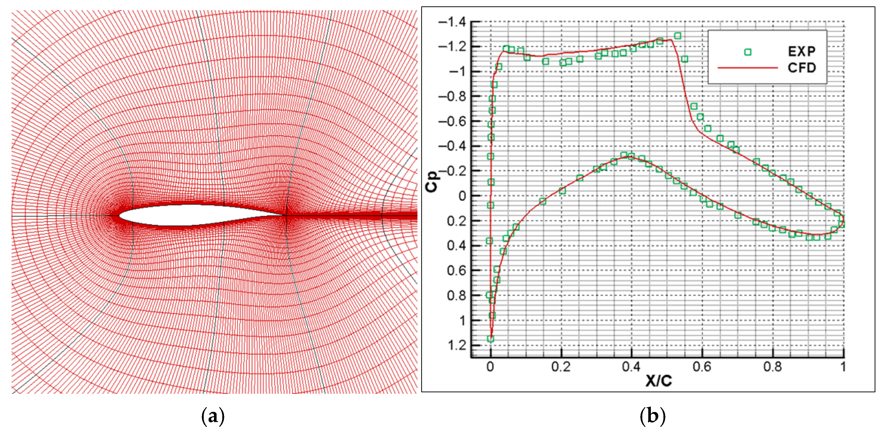
The mean and variance of the drag coefficient for each sample in design space were obtained by invoking the CFD solver to compute the drag coefficients averaged over Mach numbers ranging from 0.71 to 0.75. The solver employed the Reynolds-Averaged Navier–Stokes (RANS) equations as the numerical framework. The Roe scheme [50], a representative method of Flux Difference Splitting (FDS) in upwind schemes, was employed for spatial discretization. An implicit time-marching scheme was adopted, and for steady-state problems, the implicit approximate factorization method was employed. The turbulence model adopted is the two-equation $k-\omega$ SST model [51]. A structured mesh was utilized, and grid deformation was managed using Volumetric Spline Interpolation Techniques (VSIT) [52]. Boundary conditions include no-slip and adiabatic wall assumptions, with a zero normal pressure gradient. Riemann invariants were applied at far-field boundaries to ensure non-reflecting conditions, and symmetry boundary conditions were used to reduce computational costs. The CFD solver, implemented as an in-house code, was validated in Figure 4 through a representative transonic flow simulation over the RAE2822 airfoil.

Figure 4a shows the computational mesh of the airfoil, consisting of 80,000 grid points. Figure 4b presents a comparison between the results computed by the CFD solver and the experimental data under the conditions of $Ma=0.73$, $C_l=0.80$, $Re=6.5\times {10}^6$. As shown in Figure 4b, the CFD results agreed well with the experimental measurements, demonstrating the solver’s accuracy and providing a solid data foundation for constructing a reliable stochastic surrogate model.

3.2.3. Calculation of the Error Function

After completing sample collection and SK surrogate model fitting, it is necessary to assess the accuracy of the SK surrogate model to determine whether to output the model directly or use the infill criterion to add new samples to the training set to improve the model’s accuracy. The accuracy of the SK surrogate model was assessed using an error function, calculated using the samples from the test set.

The error function is defined as follows:

$$E={\displaystyle \frac{1}{N}}{\displaystyle \sum _{i=1}^N(O_i^{\mathrm{p}}-O_i^{\mathrm{t}})}$$

(11)

where $N$ is the number of samples in the test set, $O_i^{\mathrm{p}}$ is the predicted target value for the $i$-th sample in the test set predicted by the SK surrogate model, and $O_i^{\mathrm{t}}$ is the true target value for the $i$-th sample in the test set calculated by the CFD solver.

The formula for $O_i^{\mathrm{p}}$ is as follows:

$$O_i^{\mathrm{p}}=10Y_i^{\mathrm{mpt}}+4000\left|Y_i^{\mathrm{vpt}}\right|$$

(12)

where $Y_i^{\mathrm{mpt}}$ and $Y_i^{\mathrm{vpt}}$ are the mean and variance of the drag coefficient for the $i$-th sample in the test set predicted by the SK surrogate model, respectively. Since the mean of the drag coefficient is on the order of ${10}^{-2}$, while the variance of the drag coefficient ranges from ${10}^{-5}$ to ${10}^{-6}$, a significant difference in magnitude exists between the two. To balance this disparity, a weighting factor of 10 is assigned to the mean of the drag coefficient, and a weighting factor of 4000 is applied to the variance of the drag coefficient.

The use of absolute values ensures non-negativity of this term, preventing cancelation effects caused by potential negative values due to numerical errors.

The formula for $O_i^{\mathrm{t}}$ is as follows:

$$O_i^{\mathrm{t}}=10Y_i^{\mathrm{mtt}}+4000\left|Y_i^{\mathrm{vtt}}\right|$$

(13)

where $Y_i^{\mathrm{mtt}}$ and $Y_i^{\mathrm{vtt}}$ are the mean and variance of the drag coefficient for the $i$-th sample in the test set calculated by the CFD solver, respectively.

As the purpose of the error function is to assess the accuracy of the surrogate model, no penalty terms are included in the error function.

3.2.4. Infill Criterion

This paper enhanced the accuracy of the surrogate model by iteratively enriching the training set using an infill criterion. This enables the construction of a sufficiently accurate surrogate model with relatively few but computationally expensive CFD simulations, which directly determines the overall efficiency and feasibility of the RADO of UAV airfoils. Specifically, the EI [53] infill criterion was adopted due to its strong global search capability and scalability. The EI infill criterion quantifies the expected improvement in the vicinity of the current best solution and selects the candidate point with the highest potential to enhance the objective function performance as the next sampling point.

In each iteration of the EI infill criterion for training the SK surrogate model, a candidate sample set consisting of 100 samples—comprising only the airfoil parameter adjustments—was generated using MM-LHS. The sample with the highest EI value within the candidate set was then selected and added to the training set for retraining the SK surrogate model.

The EI value for the $k$-th candidate sample is calculated as:

$$E{I}_k=\left(f_{min}-{\mu }_k\right)\cdot \Phi \left({\displaystyle \frac{f_{min}-{\mu }_k}{{\sigma }_k}}\right)+{\sigma }_k\cdot \varphi \left({\displaystyle \frac{f_{min}-{\mu }_k}{{\sigma }_k}}\right)$$

(14)

where

$f_{min}$ is the best integrated optimization objective value for the samples in the current training set, incorporating both the optimization objective and the constraints;

${\mu }_k$ is the predicted integrated optimization objective value for the $k$-th candidate sample;

${\sigma }_k$ is the standard deviation of the prediction error for the $k$-th candidate sample;

$\Phi (\cdot )$ and $\varphi (\cdot )$ are the cumulative distribution function and probability density function of the standard normal distribution, respectively.

The best integrated optimization objective value $f_{min}$ for the samples in the current training set is defined as:

$$f_{min}=\underset{1\le j\le M}{min}(10Y_j^{\mathrm{mtT}}+4000\left|Y_j^{\mathrm{vtT}}\right|+P_j^{\mathrm{thick}}+P_j^{\mathrm{var}})$$

(15)

where

$M$ is the number of samples in the current training set;

$Y_j^{\mathrm{mtT}}$ and $Y_j^{\mathrm{vtT}}$ is the mean of the drag coefficient for the $j$-th sample in the current training set calculated by the CFD solver, respectively;

$P_j^{\mathrm{thick}}$ and $P_j^{\mathrm{var}}$ are the thickness penalty term and the variance penalty term for the $j$-th sample in the current training set calculated using the ThicknessCheck function and the VarianceCheck function, respectively.

The boundary penalty term is not included here, as it is only relevant during PPO-Clip optimization.

The predicted integrated optimization objective value ${\mu }_k$ for the $k$-th candidate sample is defined as:

$${\mu }_k=10Y_k^{\mathrm{mpc}}+4000\left|Y_k^{\mathrm{vpc}}\right|+P_k^{\mathrm{thickc}}+P_k^{\mathrm{varc}}$$

(16)

where

$Y_k^{\mathrm{mpc}}$ and $Y_k^{\mathrm{vpc}}$ are the mean and variance of the drag coefficient for the $k$-th candidate sample predicted by the SK surrogate model, respectively;

$P_k^{\mathrm{thickc}}$ and $P_k^{\mathrm{varc}}$ are the thickness penalty term and the variance penalty term for the $k$-th candidate sample calculated using the ThicknessCheck function and the VarianceCheck function, respectively.

The standard deviation of the prediction error ${\sigma }_k$ used in the EI formula is computed as:

$${\sigma }_k=\sqrt{\left|Y_k^{\mathrm{mmc}}\right|+\left|Y_k^{\mathrm{vmc}}\right|}$$

(17)

where $Y_k^{\mathrm{mmc}}$ and $Y_k^{\mathrm{vmc}}$ are the MSEs of the predicted mean and variance of the drag coefficient for the $k$-th candidate sample, respectively.

After computing the EI values for all candidate samples, the sample with the highest EI value was selected. Its true mean and variance of the drag coefficient were obtained using the CFD solver, and the corresponding thickness and variance penalty terms were calculated. These values were then added to the training set, and the SK surrogate model was retrained. This process was repeated until either the model accuracy meets the required threshold—validated by the error function—or the maximum number of iterations is reached.

3.3. The Accuracy Validation of the Stochastic Kriging Surrogate Model

After updating the SK surrogate model with 1000 initial samples and 4572 iterations using the infill criterion, the value of the error function in the test set was found to be $2.494\times {10}^{-3}$, which is smaller than the set threshold of $2.5\times {10}^{-3}$.

To evaluate the accuracy of the mean of the drag coefficient predicted by the SK surrogate model, the mean relative error is used, as defined in Equation (18):

$$MRE={\displaystyle \frac{1}{N}}{\displaystyle \sum _{i=1}^N\left|\frac{Y_i^{\mathrm{mtt}}-Y_i^{\mathrm{mpt}}}{Y_i^{\mathrm{mtt}}}\right|\times 100\%}$$

(18)

Upon verification, the mean relative error of the predicted mean of the drag coefficient was 0.329%. In engineering practice, a mean relative error of less than 1% is generally considered acceptable, which indicates that the SK surrogate model provides a good prediction for the mean of the drag coefficient.

Regarding the accuracy of the variance of the drag coefficient predicted by the SK surrogate model, since the variance values are quite small, calculating the relative error becomes unstable and can amplify the error. Therefore, the mean logarithmic error was used, as this approach compresses the differences between large and small values, making the error calculation more balanced. The formula for the mean logarithmic error is provided in Equation (19):

$$MLE={\displaystyle \frac{1}{N}}{\displaystyle \sum _{i=1}^N\left|\ln (\left|Y_i^{\mathrm{vtt}}\right|)-\ln (\left|Y_i^{\mathrm{vpt}}\right|)\right|}$$

(19)

Upon testing, the mean logarithmic error of the variance of the drag coefficient predicted by the SK surrogate model was found to be 0.056. In engineering, a mean logarithmic error of less than 0.1 is typically considered acceptable, indicating that the SK surrogate model provides good accuracy for the variance of the drag coefficient.

The SK surrogate model’s high prediction accuracy for both mean and variance of the drag coefficients provides a reliable data foundation for subsequent RADO of UAV airfoils using the PPO-clip algorithm.

4. Establishment of Robust Aerodynamic Design Optimization Process for UAV Airfoils Based on the PPO-Clip Algorithm

The PPO-Clip algorithm served as the core of RADO methodology for UAV airfoils, guiding the optimization direction. In this section, a trained SK surrogate model was used as the data foundation to establish the RADO process for UAV airfoils based on the PPO-Clip algorithm. First, the principle of the PPO-Clip algorithm was introduced. Then, a PPO-Clip-based RADO process for UAV airfoils was constructed and briefly overviewed. The architecture of the optimization environment—a key component of the RADO process—was then described. Subsequently, the state transition function and the reward function were specifically designed in accordance with the optimization objectives and constraints of the RADO problem. Finally, in order to enhance the stability and reliability of the PPO-Clip algorithm, structural modifications were applied to the algorithm.

4.1. Principle of the PPO-Clip Algorithm

The PPO-Clip algorithm is a representative policy-based RL method. It optimizes a parameterized policy, represented by a neural network, to obtain the optimal solution by applying gradient ascent to the policy loss function $L^{policy}$. The algorithm directly outputs the action probability distribution and naturally supports continuous and stochastic decision-making tasks. Given that the RADO of UAV airfoils is inherently high-dimensional, complex, and continuous, while also requiring stability during training, the PPO-Clip algorithm was adopted in this paper as the core optimization engine.

The framework of the PPO-Clip algorithm is similar to that of the Actor-Critic architecture [54], in which the Actor (i.e., the policy network) outputs actions based on the current policy, while the Critic (i.e., the value network) evaluates those actions to guide the learning process. Generalized Advantage Estimation (GAE) [55] ${\widehat{A}}_t$ is commonly employed as the advantage function to assess the performance of individual actions relative to the average under the current policy and guide policy updates accordingly. A discount factor $\gamma$ is introduced to weigh the relative importance of immediate and future rewards, while the GAE parameter $\lambda$ is used to balance the trade-off between bias and variance in the advantage function. The state-value function $V\left(s_t\right)$ is employed in this computation, and it can be obtained from the output of the value network, which is trained by minimizing the MSE between the estimated state-value function $V\left(s_t\right)$ and the temporal difference (TD) target $y_t$ as the loss function $L^{value}$.

The core idea of the PPO-Clip algorithm is to introduce a clipping mechanism during policy updates. The magnitude of policy updates is constrained using the clipped probability ratio method, with the clipping parameter $\epsilon$ controlling the allowable deviation between the new and old policies, thereby preventing instability caused by excessively large updates. Meanwhile, an entropy regularization term is employed to encourage exploration, with its strength governed by the entropy coefficient $\beta$, which helps the algorithm discover globally superior solutions in the complex UAV airfoil design space and avoid entrapment in local optima.

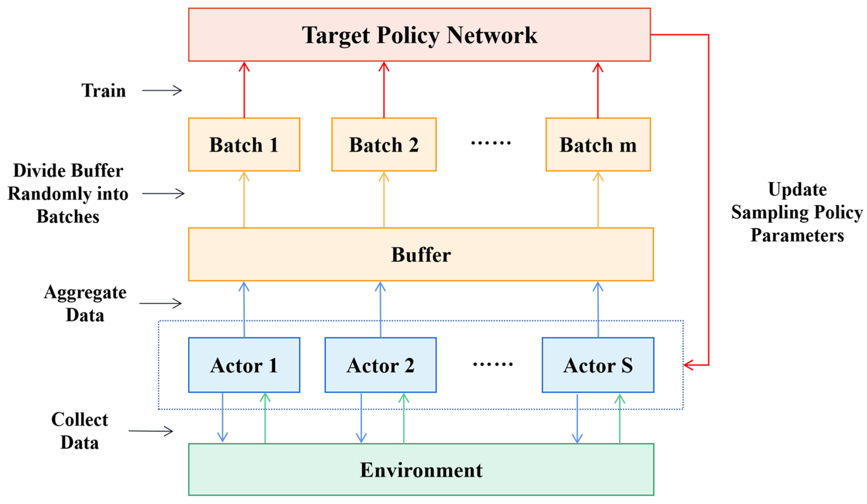
To enhance data collection efficiency and reduce variance between data points, during training consisting of a total of $N$ episodes, each with $T$ timesteps, the PPO-Clip algorithm uses $S$ actors to interact with the environment for data collection, aggregating the collected data in the buffer. During each epoch, the data in the buffer is randomly divided into multiple batches of size $B$, and the batches are iterated over to train the target policy network. This approach helps improve the generalization ability of the network model and prevent overfitting. Additionally, the updated parameters of the target policy network are transmitted to the actors to update their sampling policies, thereby enhancing the timeliness of subsequent data collection. The flowchart is shown in Figure 5.

The policy network parameters and value network parameters were updated using the Adam optimizer. Adam (Adaptive Moment Estimation) [56] is a highly efficient and adaptive optimization algorithm and is currently one of the mainstream choices.

The process of the PPO-Clip algorithm is as follows (Algorithm 1):

Algorithm 1 PPO-Clip Algorithm Process [30]

$\mathrm{Initialize} \mathrm{the} \mathrm{policy} \mathrm{network} \mathrm{parameters} {\theta }_0$$\mathrm{and} \mathrm{value} \mathrm{network} \mathrm{parameters} {\varphi }_0$.

for episode = 1, 2, 3, …, N do

for actor = 1, 2, 3, …, S do

Interact with the environment using the current policy for $T$ timesteps,

obtaining a series of states, actions, and reward data, and store them in the buffer.

$\hspace{1em}\hspace{1em} \mathrm{Compute} \mathrm{the} \mathrm{state}-\mathrm{value} \mathrm{function} V\left(s_t\right)$$, \mathrm{TD} \mathrm{target} y_t$$, \mathrm{and} \mathrm{GAE} {\widehat{A}}_t$, and store

them in the buffer.

end for

for epoch = 1, 2, 3, …,$K$ do

$\hspace{1em}\hspace{1em} \mathrm{Divide} \mathrm{the} \mathrm{data} \mathrm{in} \mathrm{the} \mathrm{buffer} \mathrm{into} \mathrm{batches} \mathrm{of} \mathrm{size} B<ST$ and iterate over each

batch:

Update the value network parameters $\varphi$$\mathrm{by} \mathrm{minimizing} L^{value}$ using the Adam

optimizer.

Update the policy network parameters $\mathrm{by} \mathrm{minimizing} L^{policy}$ using the

Adam optimizer.

end for

$\hspace{1em}{\theta }^{\prime }\leftarrow \theta$$, {\varphi }^{\prime }\leftarrow \varphi$

end for

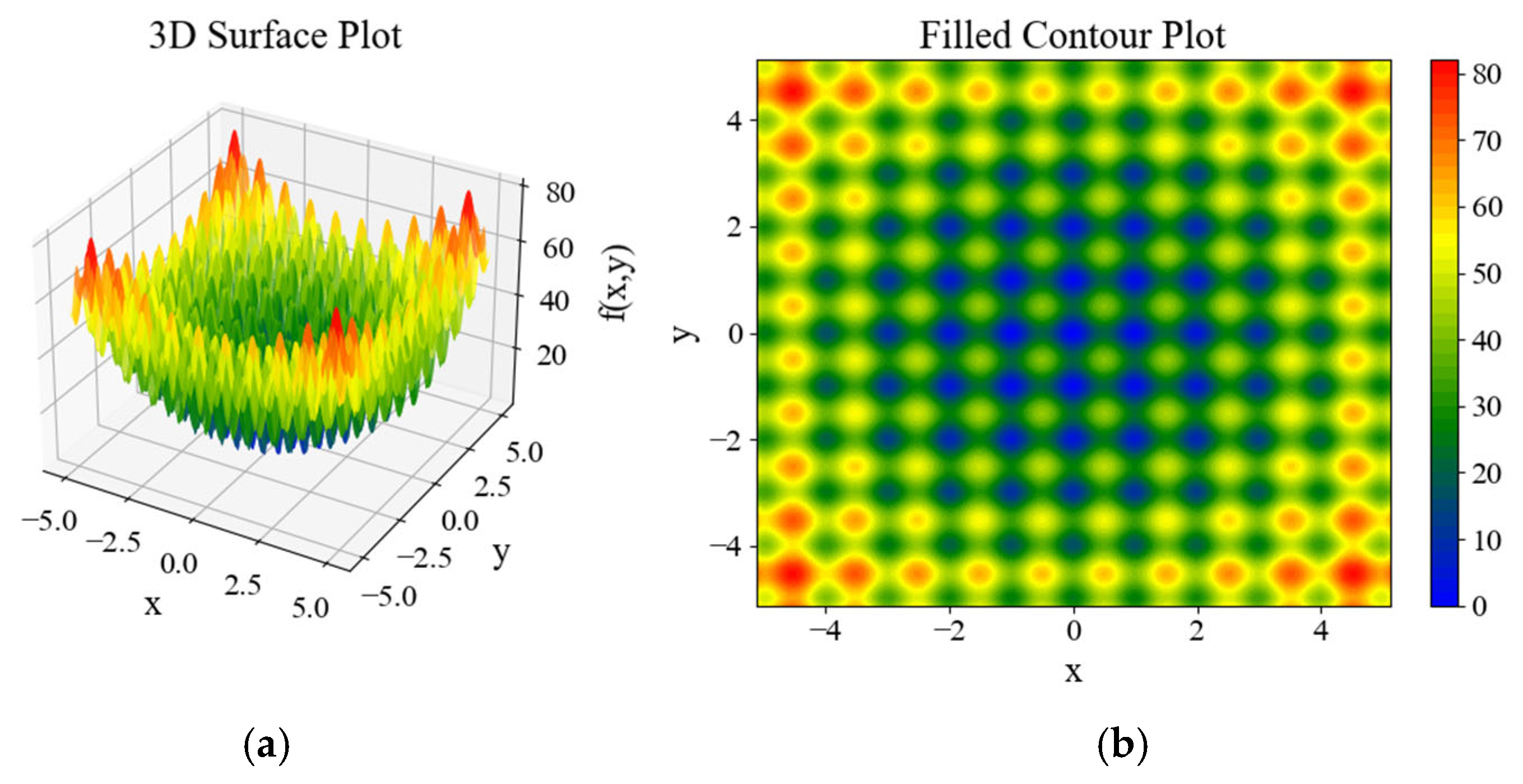
To evaluate the performance and effectiveness of the PPO-Clip algorithm, the 2D Rastrigin function [57] was employed as the benchmark function. Its mathematical expression is given as follows:

$$f(x,y)=20+x^2+y^2-10(\cos (2\pi x)+\cos (2\pi y))\hspace{1em}x,y\in [-5.12,5.12]$$

(20)

This function is widely employed for algorithm performance testing due to its highly multimodal nature, regular structure that facilitates visualization, and clearly defined global optimum at (0,0) with a function value of 0, which makes it convenient for algorithm evaluation. The 3D surface plot and filled contour plot of the function are shown in Figure 6a,b, respectively.

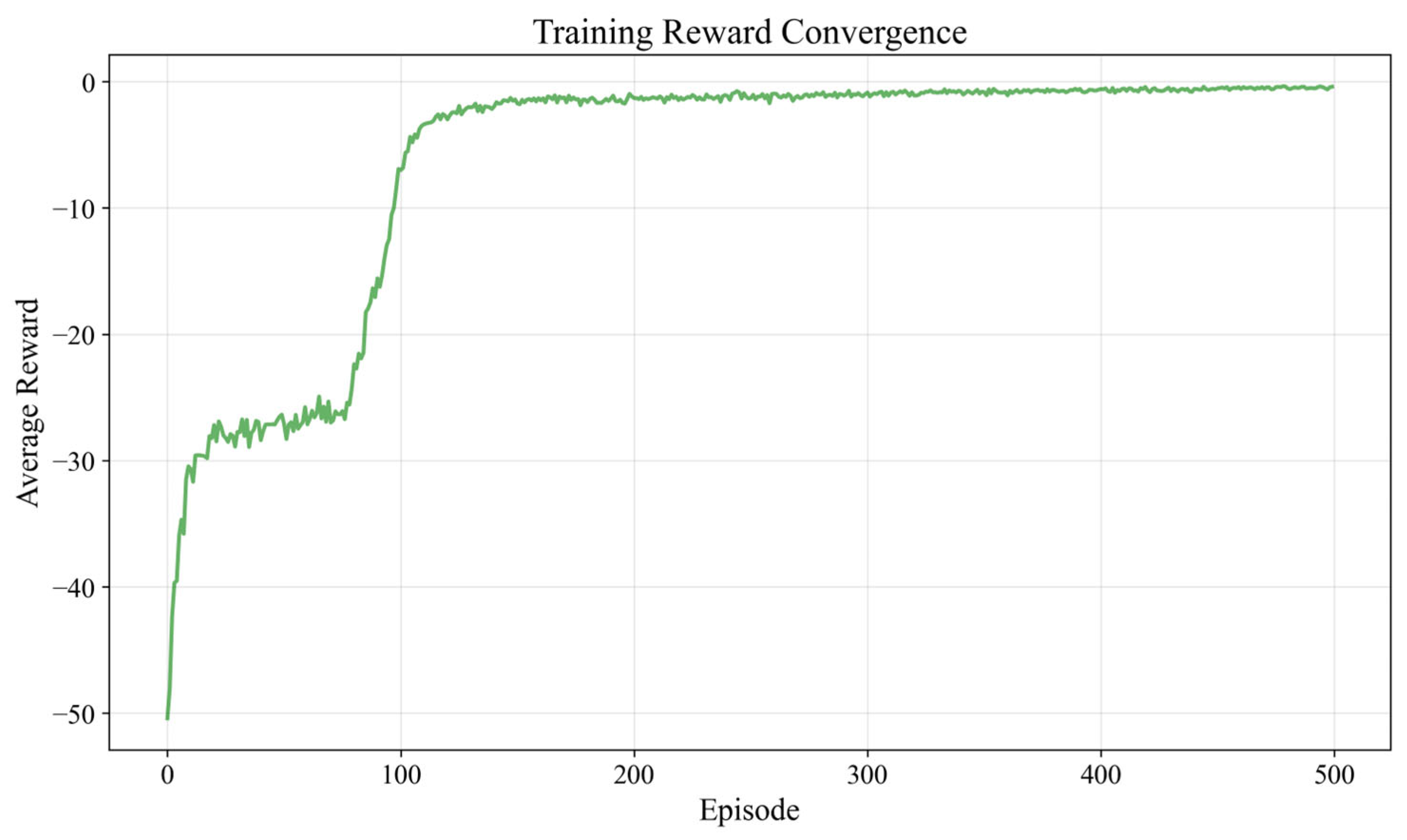
Figure 7 shows the training process of the PPO-Clip algorithm for finding the minimum of the 2D Rastrigin function, and Figure 8 illustrates the corresponding optimization process.

As shown in Figure 7, during 500 training episodes, the algorithm approached convergence by around the 400th episode. As illustrated in Figure 8, after 1.99 s of optimization, the algorithm successfully converged and identified a solution close to the theoretical global optimum at the 2nd step, thereby demonstrating the reliability and efficiency of the PPO-Clip algorithm.

4.2. Robust Aerodynamic Design Optimization Process for UAV Airfoils Based on the PPO-Clip Algorithm

4.2.1. Overview of Robust Aerodynamic Design Optimization Process for UAV Airfoils

To closely align with the practical high-dimensional optimization space in engineering, both the state space and action space were defined as continuous spaces. The state was defined as the UAV airfoil parameter adjustments (a 9-dimensional vector), and the action was the change in UAV airfoil parameter adjustments (also a 9-dimensional vector). The state space was limited to the range of $[-0.2,0.2]$. During the optimization process, Z-score normalization [58] was applied to the states to eliminate dimensional differences in the airfoil parameter adjustments, which accelerates the convergence of the policy network and value network for RADO of UAV airfoils. The action space was limited to the range of $[-1,1]$, similar to mean normalization, making it easier for the policy network to learn, and also avoiding excessively large or small action values, improving training stability. The state was reset with random initialization within the range of $[-0.2,0.2]$, instead of always starting from the same state, which enhances policy network’s exploration capabilities across distinct regions of the UAV airfoil design space.

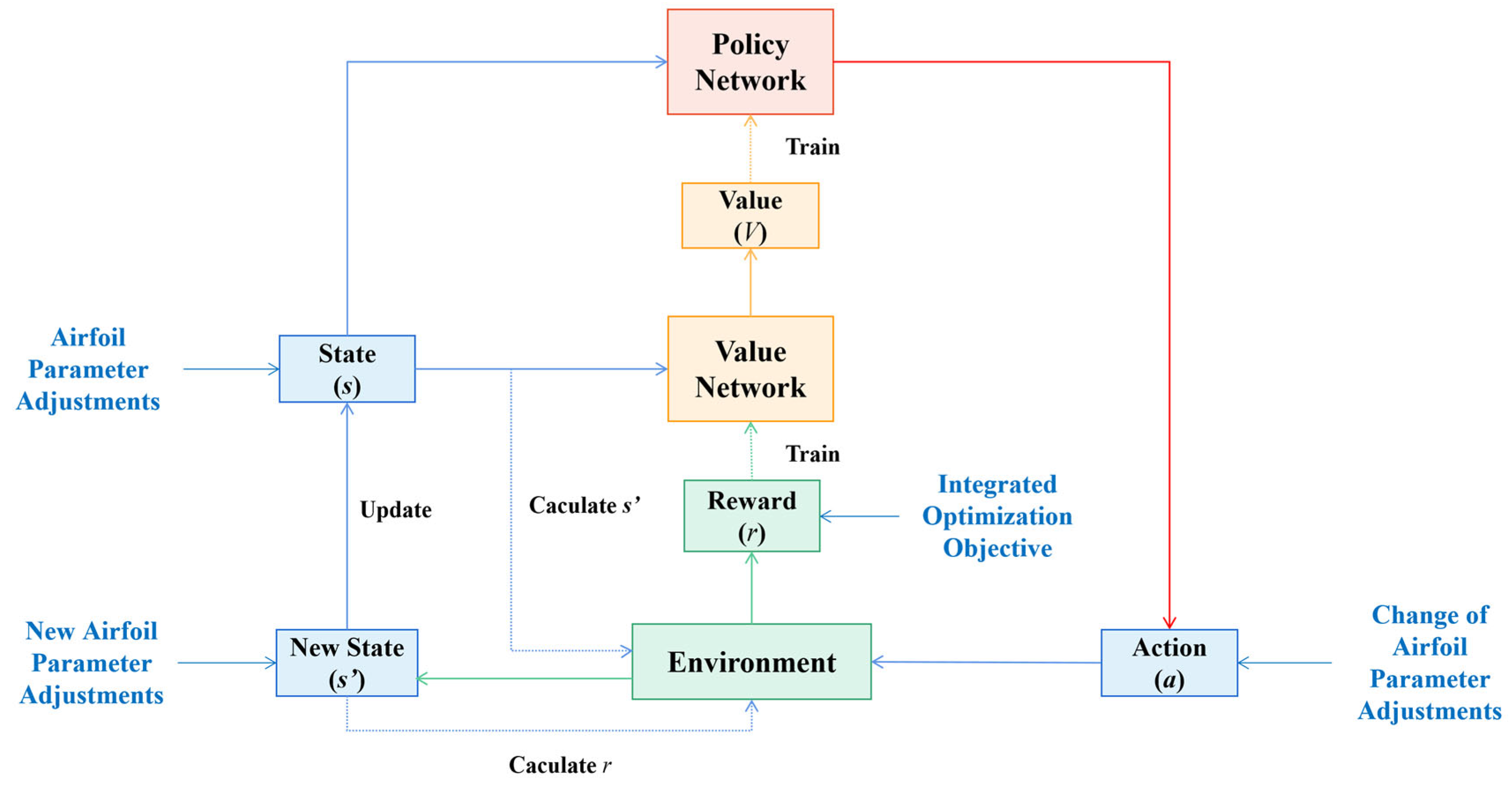
Figure 9 is the block diagram of RADO process for UAV airfoils. In the optimization process, the airfoil parameter adjustments are used as the state input into the environment. The environment, based on the state transition function, outputs a new state (new airfoil parameter adjustments) by combining the action (change in airfoil parameter adjustments). Meanwhile, the environment outputs a reward based on the reward function and the new state. The reward function is set to the integrated optimization objective. The reward provided by the environment can be used to compute the TD target value, which helps train the value network. The value output by the value network can be used to calculate the GAE, which in turn helps train the policy network. The policy network outputs action based on the input state. Through continuous interaction with the environment, the policy network is ultimately trained to maximize the expected value of the integrated optimization objective.

4.2.2. Environmental Architecture

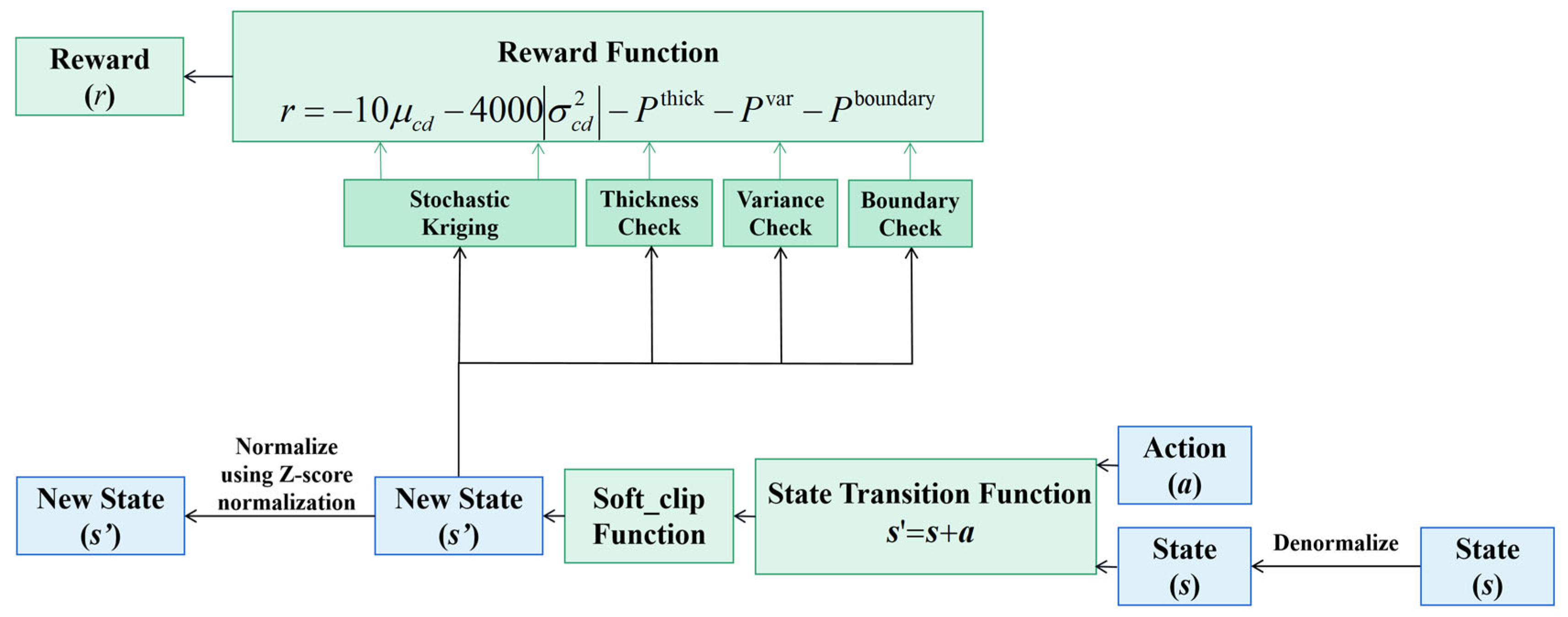
In RL, the main role of the environment is to output a new state and reward based on the agent’s state and action, combining the state transition function and reward function, thus assisting the agent in training the policy network. Consequently, the design of environmental architecture is a critical aspect of the RL framework. Within this architecture, the state transition function and reward function constitute its core components. Figure 10 is the environmental architecture diagram of RADO for UAV airfoils based on the PPO-Clip algorithm in this paper. Its core function is to evaluate the robustness performance (i.e., the reward) of a given UAV airfoil design under target flight conditions (Mach number perturbations), and to generate new design recommendations accordingly (i.e., the new state). First, the state representing the airfoil parameter adjustments, which is previously normalized using Z-score normalization, is denormalized to its original form. This restored state is then combined with the action—interpreted as the change in the airfoil parameter adjustments—through a state transition function to generate a new state, i.e., the new airfoil parameter adjustments. To prevent this new state from exceeding predefined bounds, a soft_clipping function is applied.

Since the reward function serves as the environment’s feedback to the agent’s action, it is calculated based on the outcome of the agent’s action, i.e., the new state (the new airfoil parameter adjustments). In the reward function, the soft-clipped new airfoil parameter adjustments are used to calculate the mean and variance of the drag coefficient through the SK surrogate model, the thickness penalty term through the ThicknessCheck function, the variance penalty term through the VarianceCheck function, and the boundary penalty term through the BoundaryCheck function. The final reward is then computed by integrating these components. After applying soft clipping, the resulting new state is normalized using Z-score normalization and then output for subsequent processing.

4.2.3. Design of the State Transition Function

Before applying the state transition, the Z-score normalized state is first denormalized to its original value. The state transition function is directly defined as:

$$\mathit{s}\mathbf{\prime }=\mathit{s}+\mathit{a}$$

(21)

This approach applies actions directly to the original values of the airfoil parameter adjustments, allowing the effects of the actions to be clearly reflected and directly corresponding to the parametric adjustment process of the UAV airfoil design. It is both simple and intuitive.

However, direct addition of action may cause the new state to exceed the predefined boundaries. If a hard clipping function is applied to forcibly constrain the new state within bounds, it can lead to the loss of action information, thereby limiting the exploration capability of UAV airfoil optimization. To address this, a soft clipping operation is introduced before applying Z-score normalization to the new state, allowing for soft constraint enforcement. The soft_clip function is defined as:

$$\begin{array}{l}\mathrm{soft}\_\mathrm{clip}(x)={\displaystyle \frac{limit}{\alpha }}[\ln \left(1+e^{\alpha x_{\mathrm{norm}}}\right)-\ln \left(1+e^{\alpha \left(x_{\mathrm{norm}}-1\right)}\right)\\ \hspace{1em}\hspace{1em}\hspace{1em}\hspace{1em}\hspace{1em}\hspace{1em}\hspace{1em}\hspace{1em}\hspace{1em}-\ln (1+e^{-\alpha x_{\mathrm{norm}}})+\ln (1+e^{-\alpha \left(x_{\mathrm{norm}}+1\right)})]\end{array}$$

(22)

where $limit$ is the soft clipping boundary, limiting the output within $\left[-limit,limit\right]$. The $limit$ was set to 0.2 based on the defined state space.

The input to the function is a normalized value $x_{\mathrm{norm}}$, defined as:

$$x_{\mathrm{norm}}={\displaystyle \frac{x}{limit}}$$

(23)

This normalization step maps $x$ to a dimensionless value relative to $limit$, enabling uniform handling of parameters with different scales.

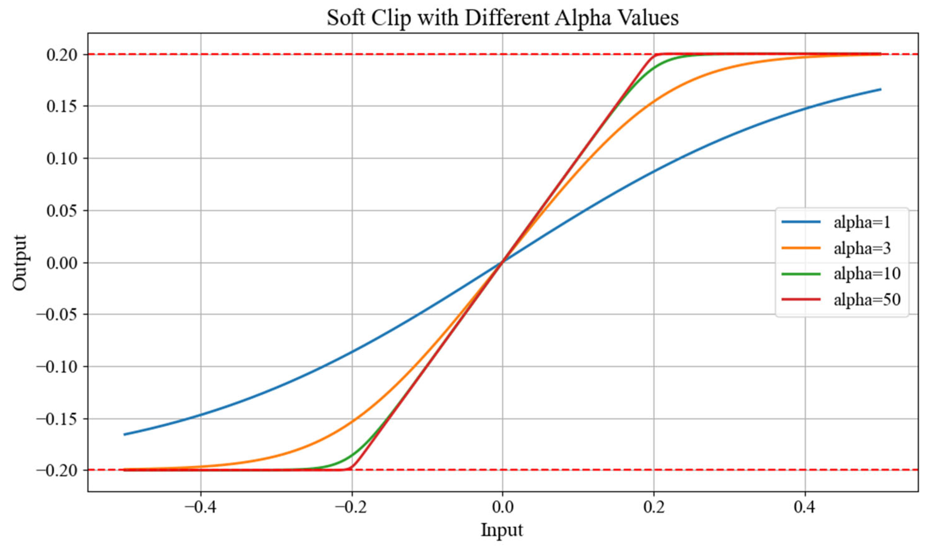
The parameter $\alpha$ controls the smoothness of the soft clipping. As shown in Figure 11, where the output bounds are set to $[-0.2,0.2]$, larger $\alpha$ values make the function approach hard clipping, while smaller values yield smoother outputs near the boundaries. To preserve gradient information and ensure smooth output near boundaries, $\alpha$ was set to 3 in this paper.

4.2.4. Design of the Reward Function

The reward function needs to be specifically designed according to the optimization objectives and constraints. A good reward function helps the policy network converge quickly and stably, ultimately satisfying the constraints and achieving the optimization objectives.

Based on the optimization objectives and constraints, the reward function is an integrated optimization objective that includes two objective terms and three constraint terms. The reward function is as follows:

$$r=-10{\mu }_{cd}-4000\left|{\sigma }_{cd}^2\right|-P^{\mathrm{thick}}-P^{\mathrm{var}}-P^{\mathrm{boundary}}$$

(24)

1.

Objective Terms

The two objective terms are minimizing the mean and variance of the drag coefficient (i.e., ${\mu }_{cd}$ and ${\sigma }_{cd}^2$), which are addressed through the weighted-sum approach in this multi-objective optimization. Minimizing the mean of the drag coefficient contributes to improving the UAV’s cruise efficiency, while minimizing the variance of the drag coefficient enhances the robustness of the UAV’s flight performance under uncertain atmospheric conditions.

2.

Constraint Terms

The three constraint terms are the airfoil thickness limit, drag coefficient variance limit, and airfoil parameter variation range limit.

The airfoil thickness limit was implemented through the ThicknessCheck function, which outputs the thickness penalty term $P^{\mathrm{thick}}$. The ThicknessCheck function is defined as follows:

$$\begin{array}{l}{\overline{c}}_{max}=max|y_{\mathrm{upper}}\left(x\right)-y_{\mathrm{lower}}\left(x\right)|\\ P^{\mathrm{thick}}=\left\{\begin{array}{cc}\begin{array}{c}10\\ 0\\ 4000\times ({\overline{c}}_{max}-0.1209)\end{array}& \begin{array}{c}{\overline{c}}_{max}<0.12\\ 0.12\le {\overline{c}}_{max}<0.1209\\ {\overline{c}}_{max}\ge 0.1209\end{array}\end{array}\right.\end{array}$$

(25)

where ${\overline{c}}_{max}=max|y_{\mathrm{upper}}\left(x\right)-y_{\mathrm{lower}}\left(x\right)|$ represents the maximum thickness difference across the chordwise positions after generating the airfoil using CST parameterization.

For airfoils with a maximum thickness less than 0.12, a fixed penalty of 10 is implemented as a hard constraint to prevent excessively thin airfoils resulting from optimization solely guided by drag coefficient reduction, thereby ensuring the structural safety of the UAV’s lightweight wings. Conversely, for airfoils exceeding a maximum thickness of 0.1209, a gradually increasing linear penalty proportional to the excess thickness is applied as a soft constraint. Combined with imposing zero penalty on airfoils possessing a maximum thickness between 0.12 and 0.1209, this strategy encourages the optimization towards thinner airfoils, indirectly guiding the process towards minimizing the drag coefficient.

The drag coefficient variance limit was enforced using the VarianceCheck function, which outputs the variance penalty term $P^{\mathrm{var}}$. The VarianceCheck function is defined as follows:

$$P^{\mathrm{var}}=\left\{\begin{array}{cc}10\hspace{1em}\mathrm{if}\hspace{1em}{\sigma }_{cd}^2<5\times {10}^{-7}\hfill & \\ 0\hspace{1em}\hspace{1em}\hspace{1em}\mathrm{otherwise}\hfill & \end{array}\right.$$

(26)

The airfoil parameter variation range limit is implemented through a soft_clip function for soft clipping, combined with the BoundaryCheck function to reduce boundary accumulation.

The soft_clip function was introduced in the design of the state transition function. Here, the BoundaryCheck function was defined to output the boundary penalty term $P^{\mathrm{boundary}}$.

The BoundaryCheck function is defined as:

$$P^{\mathrm{boundary}}=0.1\cdot {\displaystyle \sum _{i=1}^9\mathbb{I}\left(\left|s_i^{\mathrm{original}}\right|>0.195\right)}$$

(27)

where $s_i^{\mathrm{orginal}}$ is the original value of each component of the airfoil parameter adjustments before applying Z-score normalization. $\mathbb{I}\left(\cdot \right)$ is the indicator function that returns 1 if the condition inside the parentheses is true and 0 otherwise.

The meaning of the BoundaryCheck function is to apply a penalty of 0.1 to each component of the airfoil parameter adjustments whose absolute value exceeds 0.195. This aims to reduce the accumulation of parameter adjustments near the boundaries, which can hinder further optimization, and to encourage the algorithm to fully explore the interior of the UAV airfoil design space.

4.2.5. Modifications to the Algorithm Structure

To enhance the training stability and reliability of the PPO-Clip algorithm in the complex RADO of UAV airfoils, and to prevent invalid designs or resource waste caused by unstable training, this paper implemented the following modifications to the PPO-Clip algorithm structure:

1.

Huber Loss Function for Value Network to Improve Stability

To further enhance the stability of value network training, this paper employed the Huber loss function instead of the conventional MSE loss. The Huber loss function combines the advantages of MSE and Mean Absolute Error (MAE), offering greater robustness to outliers and more stable gradient behavior.

2.

Partial Layer Sharing Between Policy and Value Networks to Simplify Architecture and Improve Model Efficiency

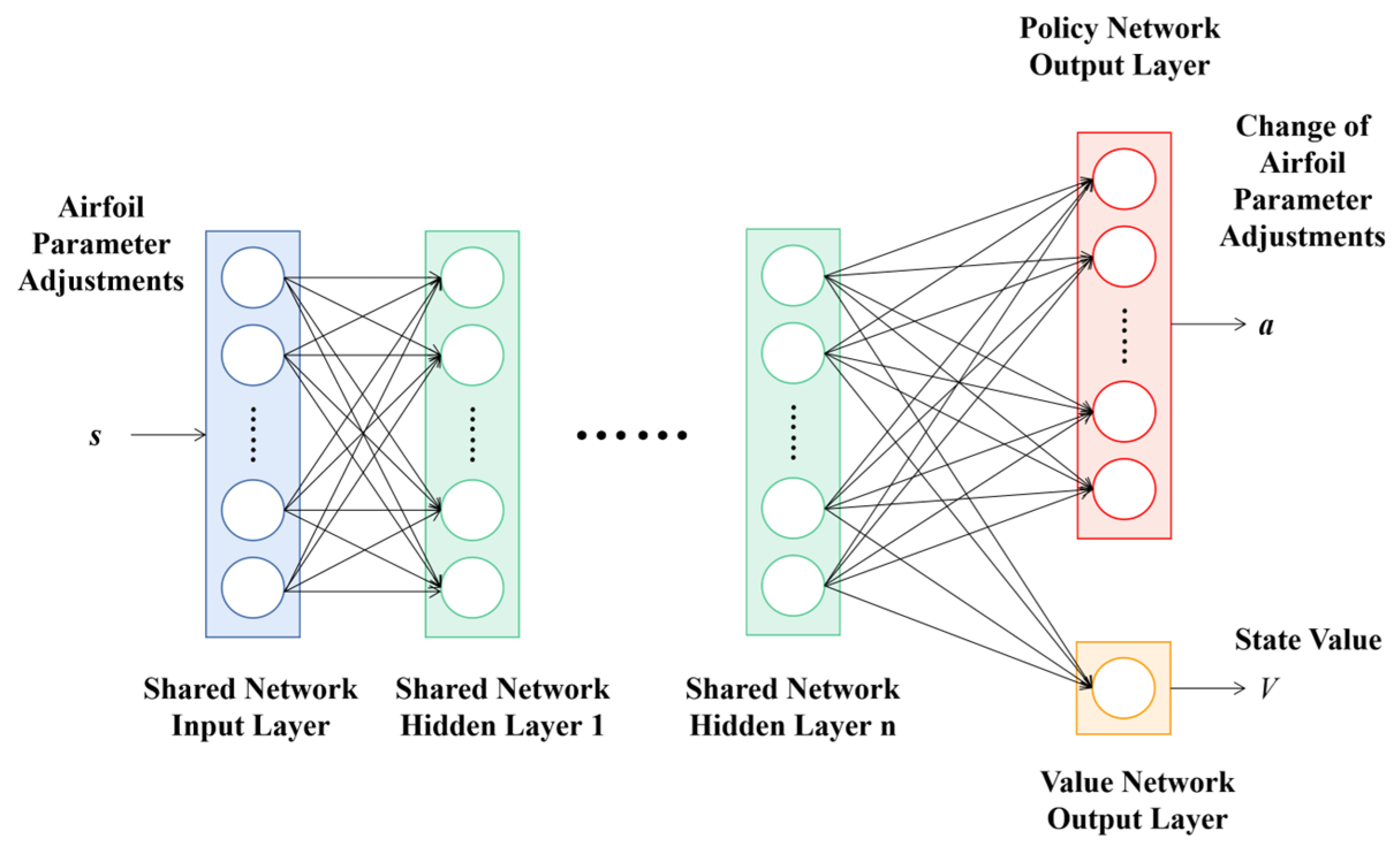
Since both the policy and value networks share the same input—the state $s$—but differ in their outputs, it is computationally efficient to share a portion of their network layers. In this design, the shared layers process the input state, after which the network branches into two separate output heads: the policy network outputs the action $a$, while the value network outputs the state value $V$. This shared architecture reduces the total number of parameters, thereby lowering computational cost and enhancing overall model efficiency. A schematic diagram of this shared network structure is presented in Figure 12.

All shared layers, policy-specific layers, and value-specific layers are implemented using fully connected (dense) layers. The specific network architecture and parameters are detailed in

Table 2. Architecture parameters of the shared, policy and value Networks.

Network Layer	Layer 1		Layer 2		Layer 3
	Neurons	Neurons	Neurons	Activation	Neurons	Activation
Shared Network Layers	256	ReLU	256	ReLU	~	~
Policy Network–Mean Layer	256	None	~	~	~	~
Policy Network–Std Layer	256	None	~	~	~	~
Value Network Layers	256	ReLU	128	ReLU	1	None

.

The policy network is divided into a mean layer and a standard deviation layer, both located at the same hierarchical level and connected to the shared network layers. The policy network samples actions from a Gaussian distribution using the outputted mean and standard deviation values.

3.

Joint Backpropagation of the Policy and Value Networks to Reduce Computational Cost

Due to the shared network layers between the policy network and the value network, to prevent the waste of computational resources caused by independent training of the two networks, this paper combined the policy network loss function and the value network loss function into a total loss function for joint backpropagation. A weighting factor of 0.5 is applied to the value loss to prioritize policy optimization.

4.

Independent Learning Rates and Schedulers for Policy and Value Networks to Enable Differentiated and Fine-tuned Optimization

This paper employed the StepLR learning rate scheduler to balance training efficiency and stability. For the distinct configurations of the policy and value networks, the policy network was assigned a relatively lower initial learning rate ${\eta }_p$ to prevent instability and policy collapse. However, to maintain sufficient exploration and avoid premature convergence to suboptimal policies, a slower decay rate was adopted, with a larger decay factor ${\gamma }_l^p$ and longer decay interval $T_s^p$. For the value network, a relatively higher initial learning rate ${\eta }_v$ was used to accelerate convergence of value estimation. To mitigate variance noise caused by overfitting in the later stages of training, a relatively fast decay rate was required, with a smaller decay factor ${\gamma }_l^v$ and shorter decay interval $T_s^v$.

Furthermore, since policy updates directly influence action selection, whereas the state-value function primarily supports policy learning, the policy network plays a dominant role in the PPO-Clip algorithm. Accordingly, the parameters of the shared layers were optimized using the policy network optimizer to ensure the extracted features are more aligned with policy learning needs. The value network optimizer was only responsible for updating the parameters exclusive to the value network.

5.

Additional Training Epochs and Weighted Processing of Historical and Current Parameters to Enhance Training Stability of the Value Network

To further enhance the training stability of the value network, after a fixed number of training epochs (denoted as $K$) for both the policy and value networks, additional training epochs (denoted as $K_v$) were conducted exclusively for the value network. This additional training ensures that the value network produces more stable state-value functions, thereby facilitating the policy network’s training.

Moreover, this paper improved robustness and mitigates the impact of outliers by prioritizing historical parameters with higher weights while downweighting current parameters, thus stabilizing the value network.

The formula for stabilizing the value network is as follows:

$${\varphi }_t\leftarrow {\alpha }_V\cdot {\varphi }_{t-1}+\left(1-{\alpha }_V\right)\cdot {\varphi }_t$$

(28)

where ${\varphi }_t$ is the value network parameters at the current timestep, ${\varphi }_{t-1}$ is the value network parameters at the previous timestep, and ${\alpha }_V$ is the smoothing coefficient for the value network, set to 0.995. By applying a weighted process to the updated parameters, drastic changes in the value network caused by single gradient updates can be reduced, thereby improving its stability.

In addition, global L2 norm gradient clipping with a threshold of 0.25 was applied to both the policy and value networks to prevent gradient explosion. Z-score normalization was applied to the GAE to enhance model stability.

4.3. Parameter Settings

The settings of the relevant parameters are shown in

Table 3. Parameter settings for the PPO-Clip algorithm.

Parameter Symbol	Parameter Value	Parameter Symbol	Parameter Value
${\eta }_p$	0.00001	$\epsilon$	0.1
${\eta }_v$	0.00002	$\beta$	0.1
${\gamma }_l^p$	0.98	$N$	1000
${\gamma }_l^v$	0.95	$T$	128
$T_s^p$	100	$S$	8
$T_s^v$	80	$B$	256
$\gamma$	0.99	$K$	10
$\lambda$	0.95	$K_v$	3

.

5. Optimization Results and Analysis

In this section, the trained SK surrogate model and the modified PPO-Clip algorithm were used to perform RADO of the commonly adopted RAE2822 airfoil for UAVs under Mach number perturbation. The computing platform used is equipped with an NVIDIA GTX 1660Ti graphics card. The software versions used are Python 3.7.16 and Torch 1.9.0+cu111. After training, the convergent reward function curve was obtained. After optimization, the convergent reward variation curve, airfoil thickness variation curve, mean of the drag coefficient variation curve and variance of the drag coefficient variation curve were achieved. Under the constraint of a constant lift coefficient, both the mean and variance of the drag coefficient were reduced, thus verifying the effectiveness of the methodology. A comparison with L-BFGS-B and PSO algorithms demonstrated the reliability and efficiency of the PPO-Clip algorithm. Finally, the reliability of the optimization results was theoretically validated by analyzing the pressure coefficient distributions and pressure contour plots of the RAE2822 airfoil and the optimized airfoil. Furthermore, the robustness of the optimization outcomes was theoretically demonstrated by examining the drag coefficient divergence characteristic curves of the RAE2822 airfoil, the deterministic optimized airfoil, and the robust optimized airfoil.

5.1. Optimization Results

5.1.1. Convergence During Training

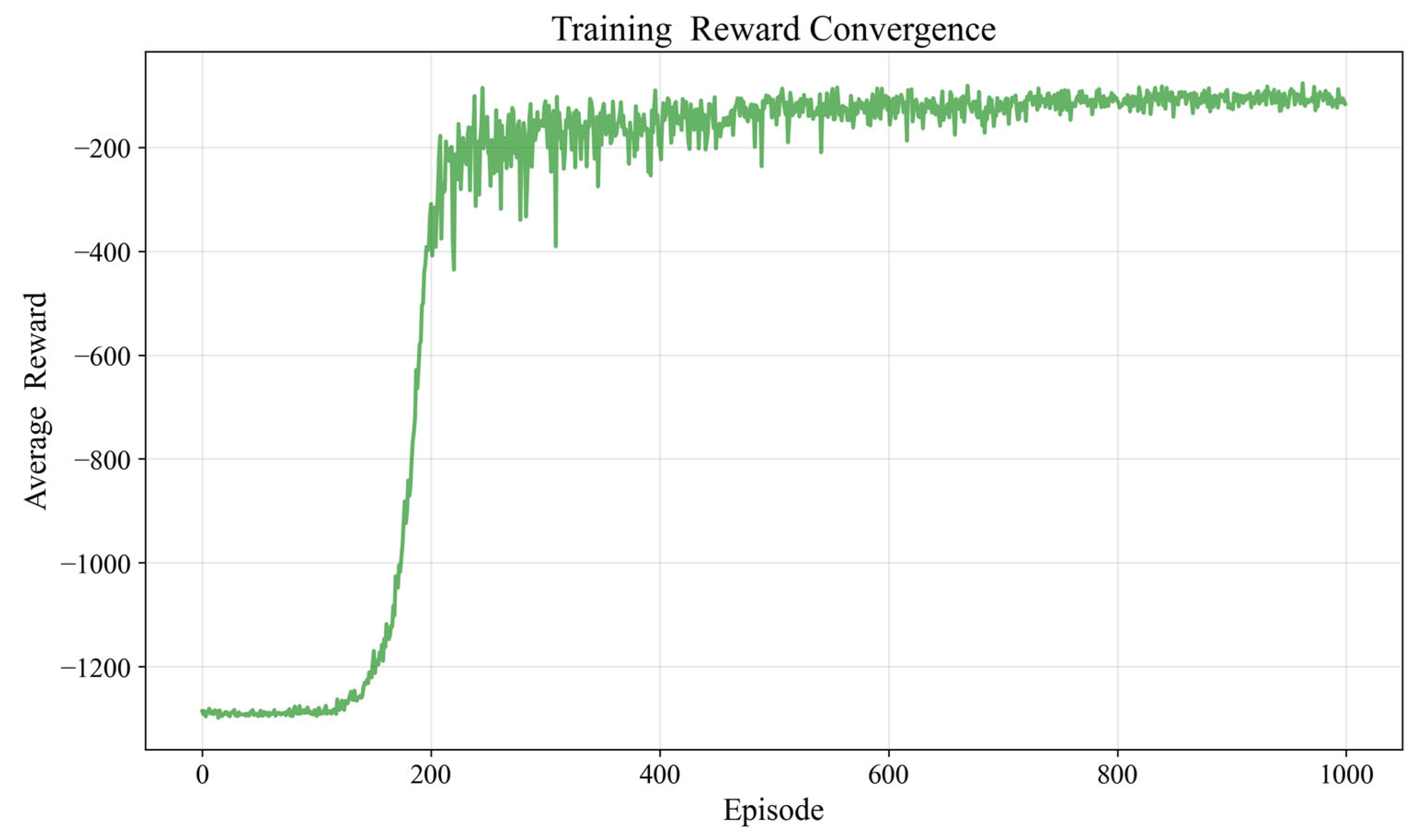
Figure 13 presents the reward function curve with respect to training episode counts. In the reward function curve, the reward represents the average reward of the sampling actors within one episode.

From Figure 13, it can be seen that the reward function nearly converged by around the 800th episode during the 1000-episode training process. This indicates that the PPO-Clip algorithm exhibits strong stability and convergence, demonstrating its feasibility and suitability for the RADO of UAV airfoils.

5.1.2. Convergence During Optimization

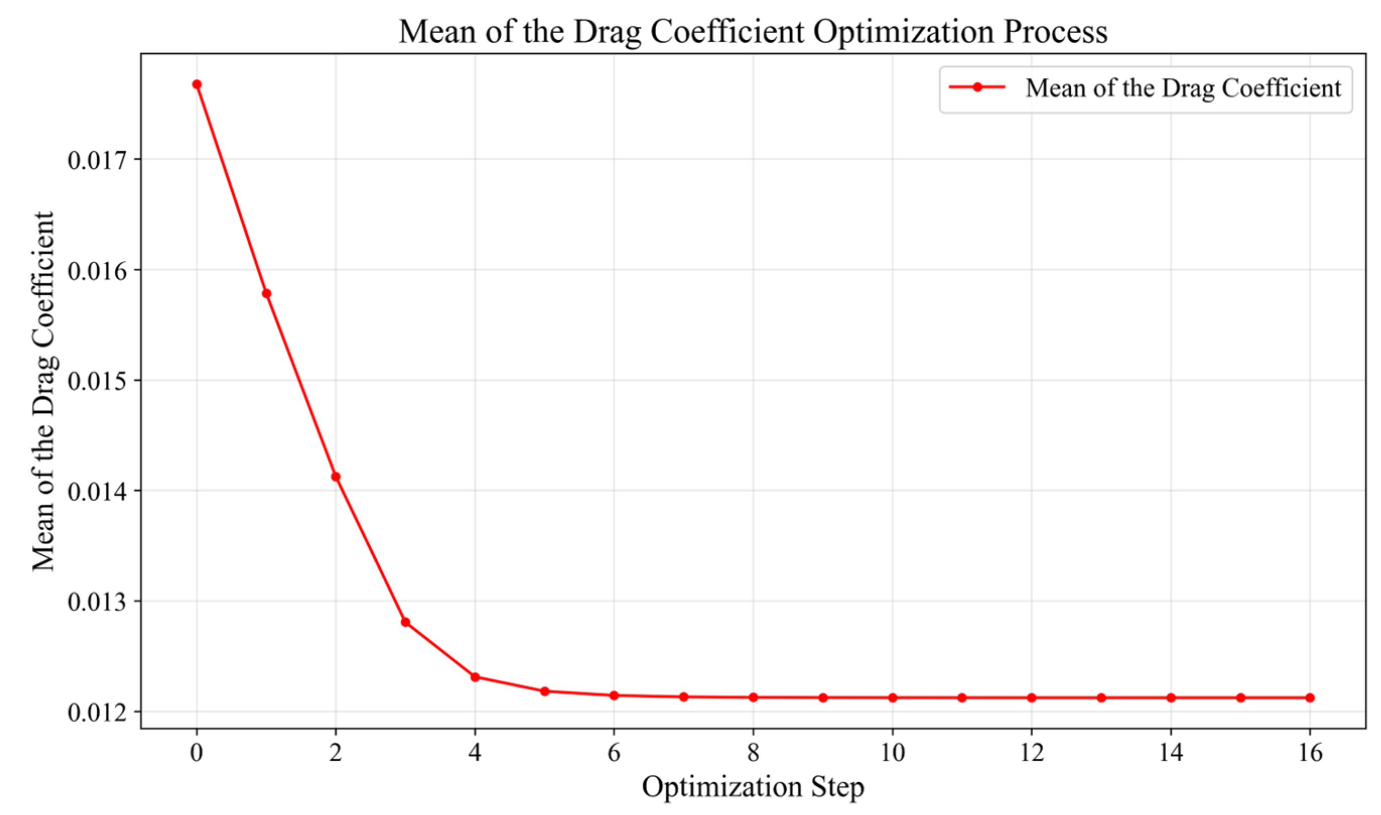
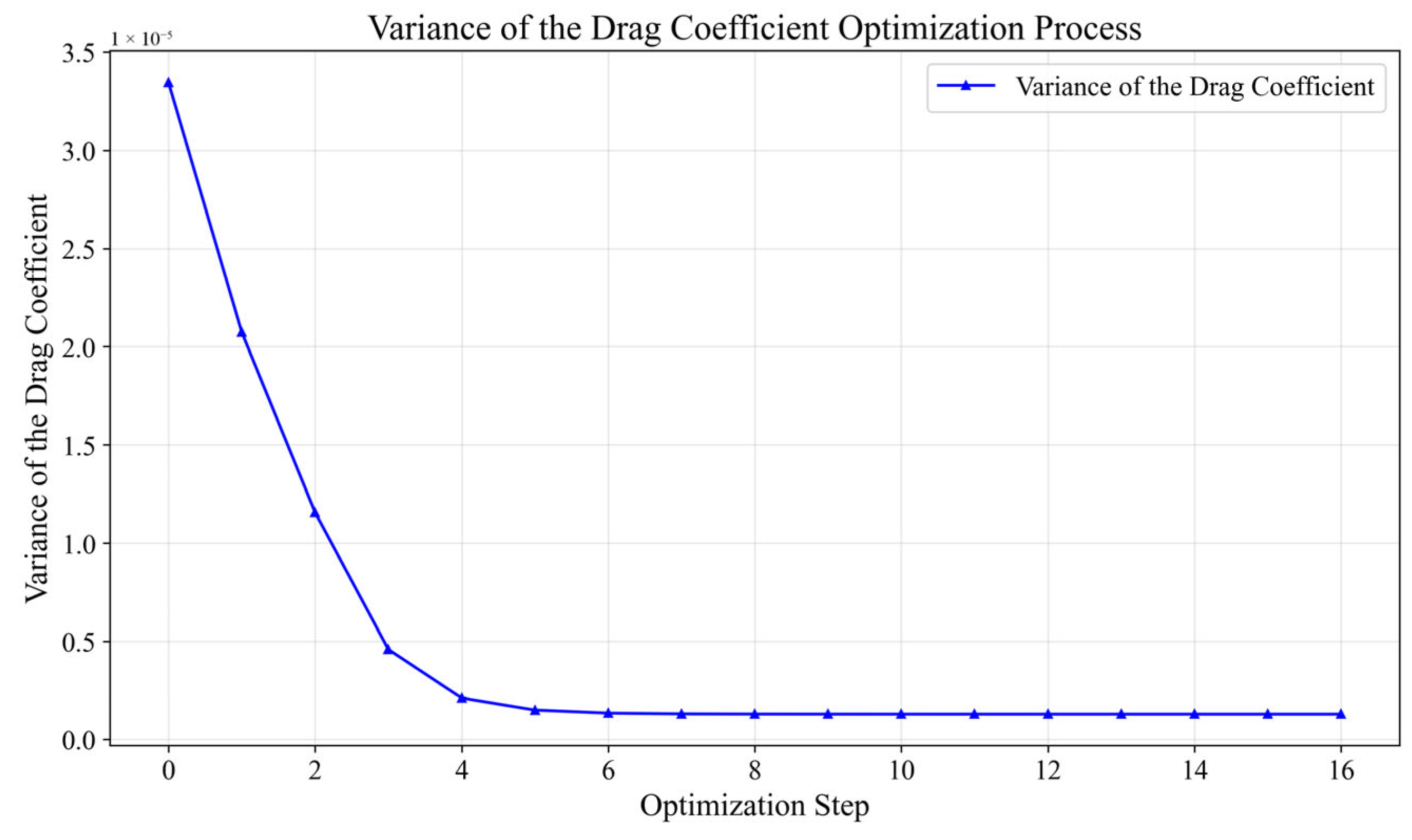
The variations in reward, airfoil thickness, mean of the drag coefficient and variance of the drag coefficient with respect to optimization steps during the optimization process are shown in Figure 14, Figure 15, Figure 16 and Figure 17. The optimization process was terminated when the reward remains unchanged for five consecutive time steps.

As shown in Figure 14, the reward value of the airfoil increased continuously during the optimization process and eventually stabilized at convergence. According to the optimization history, the maximum reward of –0.42636 was achieved at step 12. Figure 15 demonstrates that the airfoil thickness converged during the optimization, with the thickness reaching 0.12053, thereby satisfying the thickness constraint. As illustrated in Figure 16 and Figure 17, both the mean and variance of the drag coefficient converged as the optimization progressed. Specifically, the mean drag coefficient converged to 0.01212, and the variance converged to $1.29\times {10}^{-6}$, fulfilling the variance constraint. The optimization process curves indicate that the PPO-Clip algorithm can stably and efficiently accomplish the RADO of UAV airfoils, achieving performance improvements while satisfying all engineering constraints.

5.1.3. Satisfactory Optimization Results

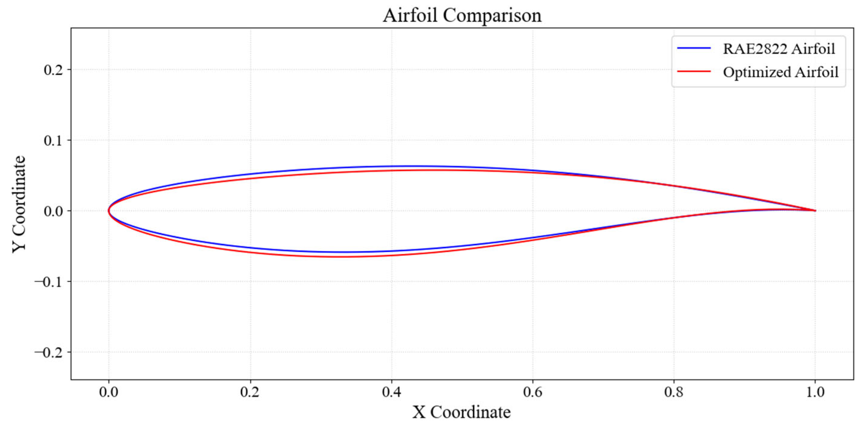
Figure 18 presents a comparison between the optimized airfoil and the baseline airfoil, RAE2822.

As shown in Figure 18, the optimized airfoil exhibited noticeable geometric modifications compared to the baseline RAE2822 airfoil. The overall camber is slightly reduced, particularly with a decrease in upper surface curvature in the mid-to-aft region. The rear loading is enhanced, the leading-edge radius is slightly reduced with a sharper profile, and the thickness near the aft spar position is marginally increased.

According to

Table 4. Optimization results.

Optimization Project	RAE2822 Airfoil	Optimized Airfoil	Degree of Optimization
Mean of the Drag Coefficient	0.01399	0.01212	−13.37%
Variance of the Drag Coefficient	$1.20\times {10}^{-5}$	$1.29\times {10}^{-6}$	−89.25%

, after optimization using the PPO-Clip algorithm, the mean of the drag coefficient for the optimized airfoil was 0.01212, representing a 13.37% reduction compared to the RAE2822 airfoil. This significantly enhances the UAV’s cruise efficiency, which can be directly translated into longer endurance or greater payload capacity. Additionally, the variance of the drag coefficient of the optimized airfoil was $1.29\times {10}^{-6}$, showing an 89.25% decrease relative to the RAE2822 airfoil. This greatly improves the robustness of the UAV airfoil’s performance under Mach number perturbations, thereby increasing the reliability and flight quality of the UAV when operating in complex atmospheric conditions.

Moreover, the optimized airfoil parameters and their corresponding adjustments were presented in

Table 5. Optimized airfoil parameters and corresponding adjustments.

Parameter Names	Corresponding Values
Optimized Airfoil Parameters	1.080617 1.332220 1.889697 2.146250 −1.379669 −1.837306 −1.954654 −1.337835 0.796404
Optimized Airfoil Parameter Adjustments	−0.178904 −0.185846 −0.187207 0.199961 −0.199981 −0.165431 −0.196841 −0.126897 0.194841

.

Figure 19 compares the optimized airfoils using the PPO-Clip, L-BFGS-B and PSO algorithm.

Table 6. Comparative analysis of optimization cost time and results.

Algorithm Name	Optimization Cost Time	Optimization Results
		Mean	Variance
PPO-Clip Algorithm	3.90 s	0.01212	$1.29\times {10}^{-6}$
L-BFGS-B Algorithm	115.35 s	0.01212	$1.69\times {10}^{-6}$
PSO Algorithm	1169.14 s	0.01214	$1.29\times {10}^{-6}$

presents a comparative analysis of optimization cost time and results obtained by these methods.

As shown in Figure 19, the airfoils optimized by L-BFGS-B and PPO-Clip exhibited broadly consistent aerodynamic profiles. However, the L-BFGS-B optimized airfoil featured a slightly sharper leading and trailing edge, a relatively flatter upper surface, and a smoother lower surface. The airfoils optimized by PSO and PPO-Clip were very similar in overall shape, with nearly identical profiles at the leading and trailing edges, and an almost perfect match on the upper surface. However, on the lower surface, the PPO-optimized airfoil showed more pronounced curvature variations and a fuller forward-mid section.

As shown in Table 6, under the condition of achieving comparable optimization results, the PPO-Clip algorithm used in this paper required significantly less computational time, being nearly 30 times faster than the L-BFGS-B algorithm and two orders of magnitude more efficient than the PSO algorithm. This clearly demonstrated the substantial advantage of the proposed methodology in addressing computationally intensive RADO problems for UAVs, enabling rapid design iterations. This efficiency gain is attributed to the PPO-Clip algorithm’s ability to directly output action from the trained policy network based on the current state, with the state subsequently updated by the environment. Compared with gradient-based optimization algorithms, it avoids the additional computational overhead of gradient evaluations while exhibiting superior global search capability. In contrast to heuristic optimization algorithms, it eliminates the need to compute and compare multiple candidate design points within a single optimization iteration, thereby reducing computational cost.

5.2. Result Analysis

5.2.1. Error Analysis of the SK Surrogate Model

Table 7. Comparison of true and predicted values of mean and variance of drag coefficient.

Optimization Project	True Value	Predicted Value	Error
Mean of the Drag Coefficient	0.01206	0.01212	0.4975%
Variance of the Drag Coefficient	$1.34\times {10}^{-6}$	$1.29\times {10}^{-6}$	0.0380

presents a comparison between the true values of the mean and variance of drag coefficients calculated using the CFD solver and the predicted values from the SK surrogate model under Mach numbers ranging from 0.71 to 0.75 for the optimized airfoil. As shown in the table, the relative error for the mean of the drag coefficient predicted by the SK surrogate model was within 0.4975%, and the logarithmic error for the variance of the drag coefficient predicted by the SK surrogate model was 0.0380. The high accuracy of the SK surrogate model ensures the reliability of the PPO-Clip optimization results for practical UAV applications.

5.2.2. Analysis of Pressure Distribution

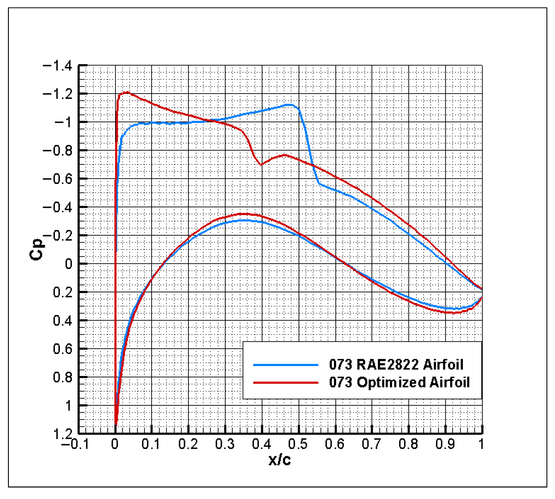
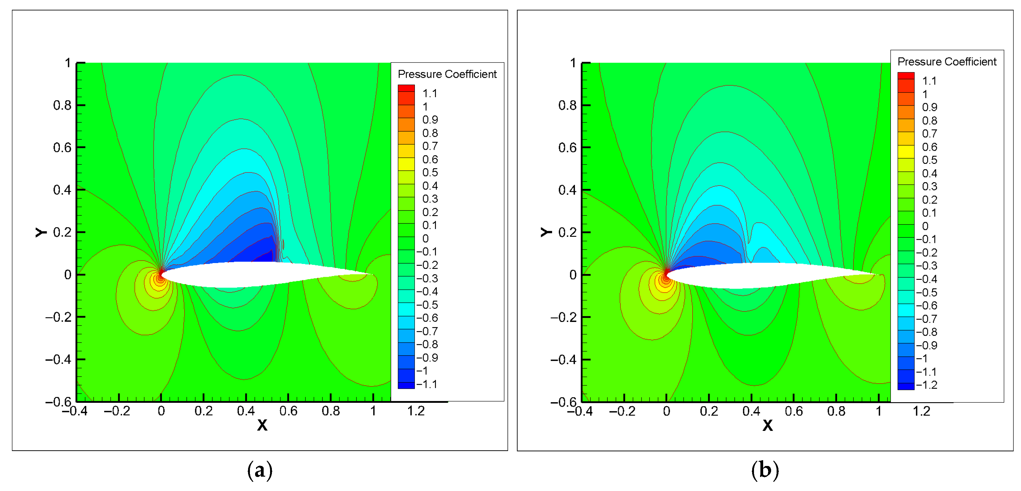
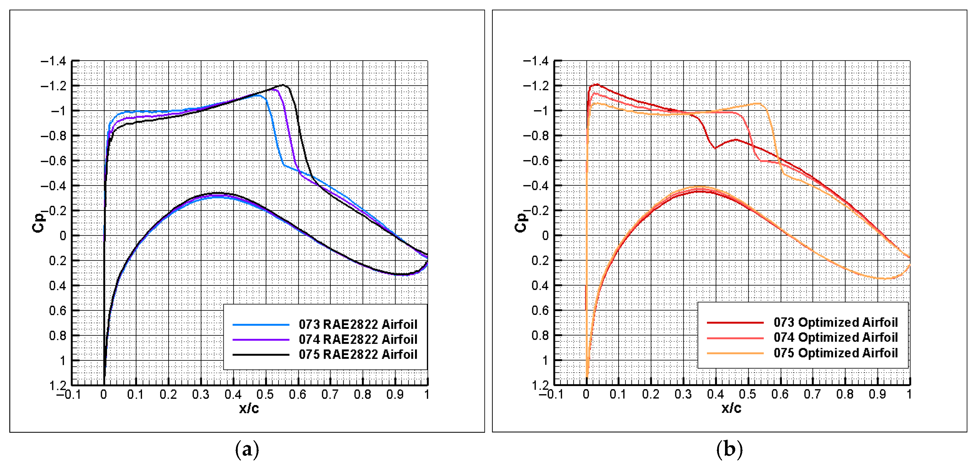
Figure 20 shows the pressure coefficient distribution comparison between the RAE2822 airfoil and the optimized airfoil, taking $Ma=0.73$ as an example. Figure 21a,b displays the pressure contour plots of the RAE2822 airfoil and the optimized airfoil at the same Mach number. Figure 22a,b, respectively, illustrates the variation in pressure coefficient distribution with increasing Mach number for the RAE2822 airfoil and the optimized airfoil.

As shown in Figure 20, at a Mach number of 0.73, the baseline RAE2822 airfoil exhibited a strong shock wave near the 50% chord position. After optimization, the optimized airfoil demonstrated a weakened shock while still satisfying the thickness constraint. Additionally, the optimized airfoil exhibited an increased suction peak at the leading edge, followed by a compression of the flow around the 40% chord, a secondary acceleration, and a gradual recovery beyond the 50% chord. This indicates that the optimization effectively improved the flow field structure of the UAV during cruise conditions. The pressure contour plots in Figure 21a,b, before and after optimization, respectively, further confirmed these observations

As illustrated in Figure 22a, the pressure coefficient of the RAE2822 airfoil exhibited a sharp intensification of shock waves with increasing Mach number, leading to a steep rise in the drag coefficient and poor drag coefficient divergence characteristics.

As shown in Figure 22b, a compression–acceleration–recovery pattern was observed at the design point. Consequently, as the Mach number increased while maintaining a constant lift coefficient, the cruise angle of attack decreased, and the leading-edge suction peak gradually diminished. Meanwhile, the compression region shifted downstream and evolved into a weak shock. As the Mach number continued to increase, this weak shock moved further aft and slightly intensified, while the typical shock–boundary layer interaction region became significantly weakened, indicating that the optimized airfoil exhibits excellent shock control capabilities, which contributes to a reduction in the drag coefficient.

Overall, compared to the RAE2822 airfoil, the optimized airfoil maintained a smooth pressure distribution across a range of Mach numbers, with mild shock evolution. This is critical for ensuring performance stability of the UAV during high-speed flight or when encountering wind shear.

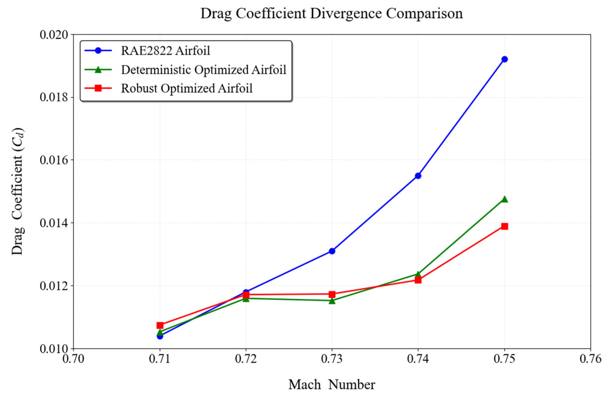
5.2.3. Analysis of Drag Coefficient Divergence Characteristics

Figure 23 presents the drag coefficient divergence characteristic curves of the RAE2822 airfoil, the deterministic optimized airfoil, and the robust optimized airfoil obtained above, within the Mach number range of 0.71–0.75. The drag coefficients are computed using a CFD solver. The deterministic optimization refers to a single-point optimization of the RAE2822 airfoil under the previously mentioned constraints, including constant lift coefficient limit, airfoil thickness limit, and airfoil parameter variation range limit, with the objective of minimizing the drag coefficient at Mach 0.73.

As shown in Figure 23, the airfoil obtained through robustness optimization exhibited a smaller degree of drag coefficient divergence compared with both the original RAE2822 airfoil and the deterministic optimized airfoil at Mach 0.73. Its drag coefficient divergence characteristic curve was flatter and more concentrated, providing direct evidence of its favorable robustness. It implies that when the UAV experiences Mach number fluctuations near cruise speed, the drag variation is reduced, resulting in a more stable flight condition, which is beneficial for flight control and mission execution.

6. Conclusions

To address the issues of high computational cost for uncertainty analysis and the inefficiency of conventional optimization algorithms in RADO of UAVs, this paper proposed a novel RADO methodology that replaces complex CFD UQ with the SK surrogate model and uses the PPO-Clip RL algorithm for optimization. The feasibility of this methodology was validated through the RADO of the widely used RAE2822 airfoil for UAVs under Mach number perturbations. First, the SK surrogate model was introduced and constructed. Then, the MM-LHS combined with the EI infill criterion was used to train the SK surrogate model and its accuracy was subsequently validated. Next, the basic concepts of the PPO-Clip algorithm were presented. Following this, the RADO process for UAV airfoils based on the PPO-Clip algorithm was established, including the design of the environmental architecture as well as the corresponding state transition function and reward function, and the use of the soft_clip function for soft boundary clipping. The structure of the PPO-Clip algorithm was also modified to improve its stability and reliability. Finally, the typical UAV airfoil RAE2822 was subjected to RADO, and the results were analyzed. The reward function curve converged during training, and the optimization curves for reward, airfoil thickness, mean of the drag coefficient, and variance of the drag coefficient also demonstrated convergence, confirming the feasibility of the PPO-Clip algorithm for this problem. The optimized design, while meeting stringent UAV engineering constraints, significantly improved key performance metrics: under the constraint of a constant lift coefficient, the mean of the drag coefficient was reduced by 13.37%, and the variance of the drag coefficient by 89.25%, substantially enhancing cruise efficiency, which contributes to increased range, payload capacity, and mission reliability. Moreover, in achieving comparable optimization results, the PPO-Clip algorithm was nearly 30 times faster than the L-BFGS-B algorithm and two orders of magnitude more efficient than the PSO algorithm, providing a powerful tool for rapid robust UAV design. The reasons behind the drag reduction were further analyzed through pressure coefficient distributions and pressure contour plots, while the robustness of the optimization results was validated through the drag coefficient divergence characteristic curves.

Although progress has been made in the RADO of UAV airfoils based on AI algorithms, there is still room for further exploration and practice in stochastic surrogate model training, high-dimensional test cases and Robust Aerodynamic/Multidisciplinary Design Optimization (RAMDO) for UAVs. In practice, it was found that each iteration for training the SK surrogate model took approximately 92 s. While fully automatable, the total training time remains lengthy—partly due to the outdated i7-9750h CPU used for CFD solver computations, and partly because of excessive sample increments and suboptimal infill criteria. Therefore, a novel three-phase sequential design of experiments methodology can be developed specifically for the SK surrogate model to reduce sample requirements, while leveraging supercomputing resources to accelerate CFD solver calculations, thereby shortening training time. In terms of test cases, this paper optimized a 2D UAV airfoil, and future research could extend this to higher-dimensional cases, such as 3D UAV wings or full aircraft, by combining the FFD parameterization method for RADO. The design variables will be significantly higher, posing more stringent demands on the reliability of the SK surrogate model and the efficiency of the PPO-Clip algorithm. In RAMDO, propulsion system requirements can be integrated by considering engine inlet performance and aerodynamic interference, enabling more comprehensive and robust optimization strategies.

Based on the progress already achieved in 2D airfoil RADO using the SK surrogate model and the PPO-Clip algorithm, research will be continued into experimental design methodologies for SK surrogate models, 3D wing/full aircraft RADO and RAMDO with the goal of developing more advanced robust design methodologies for next-generation high-performance, high-reliability UAVs.

References

1. Yao, W.; Chen, X.; Luo, W.; van Tooren, M.; Guo, J. Review of uncertainty-based multidisciplinary design optimization methods for aerospace vehicles. Prog. Aerosp. Sci. 2011, 47, 450–479. [Google Scholar] [CrossRef]
2. Zang, T.A.; Hemsch, M.J.; Hibburger, M.W.; Kenny, S.P.; Luckring, J.M.; Maghami, P.; Padula, S.L.; Stroud, W.J. Needs and Opportunities for Uncertainty-Based Multidisciplinary Design Methods for Aerospace Vehicles; NASA/TM-2002-211462; NASA Langley Research Center: Hampton, VA, USA, 2002. [Google Scholar]
3. Wang, B. Stochastic Kriging Modeling Method and Its Application in Aerodynamic Design of Aircraft. Ph.D. Thesis, Northwestern Polytechnical University, Xi’an, China, 2013. (In Chinese). [Google Scholar]
4. Taguchi, G.; Chowdhury, S.; Taguchi, S. Robust Engineering: Learn How to Boost Quality While Reducing Costs & Time to Market; McGraw-Hill: New York, NY, USA, 2000. [Google Scholar]
5. Padula, S.L.; Li, W. Options for robust airfoil optimization under uncertainty. In Proceedings of the 9th AIAA/ISSMO Symposium on Multidisciplinary Analysis and Optimization, Atlanta, GA, USA, 4–6 September 2002; AIAA: Reston, VA, USA. [Google Scholar] [CrossRef]
6. Keane, A.J. Cokriging for robust design optimization. AIAA J. 2012, 50, 2351–2364. [Google Scholar] [CrossRef]
7. Zhao, H.; Gao, Z.; Gao, Y.; Wang, C. Effective robust design of high lift NLF airfoil under multi-parameter uncertainty. Aerosp. Sci. Technol. 2017, 68, 530–542. [Google Scholar] [CrossRef]
8. Zhao, H.; Gao, Z.H. Uncertainty-based design optimization of NLF airfoil for high altitude long endurance unmanned air vehicles. Eng. Comput. 2019, 36, 971–996. [Google Scholar] [CrossRef]
9. Zhao, H.; Gao, Z.H.; Xu, F.; Zhang, Y.D. Review of robust aerodynamic design optimization for air vehicles. Arch. Comput. Methods Eng. 2019, 26, 685–732. [Google Scholar] [CrossRef]
10. Zhao, H.; Wang, S.K.; Gao, Z.H.; Huang, J.T. Research progress of robust aerodynamic optimization methods for aircraft. Acta Aerodyn. Sin. 2024, 42, 35–69. (In Chinese) [Google Scholar] [CrossRef]
11. Xue, Z.; Marchi, M.; Parashar, S.; Li, G. Comparing Uncertainty Quantification with Polynomial Chaos and Metamodels-Based Strategies for Computationally Expensive CAE Simulations and Optimization Applications; SAE Technical Papers: Warrendale, PA, USA, 2015. [Google Scholar]
12. Ghanem, R.; Spanos, P. Stochastic Finite Elements: A Spectral Approach; Dover Publications: Mineola, NY, USA, 2003. [Google Scholar]
13. Lacor, C.; Savin, É. General introduction to polynomial chaos and collocation methods. In Uncertainty Management for Robust Industrial Design in Aeronautics; Springer: Cham, Switzerland, 2019; pp. 109–122. [Google Scholar]
14. Volpi, S.; Diez, M.; Gaul, N.J.; Song, H.; Iemma, U.; Choi, K.K.; Campana, E.F.; Stern, F. Development and validation of a dynamic metamodel based on stochastic radial basis functions and uncertainty quantification. Struct. Multidiscip. Optim. 2014, 51, 347–368. [Google Scholar] [CrossRef]
15. Wang, B.; Bai, J.; Ge, H.C. Stochastic Kriging for random simulation metamodeling with finite sampling. In Proceedings of the 39th ASME Design Automation Conference, Portland, OR, USA, 5–8 August 2013. [Google Scholar]
16. Wang, B.; Gea, H.; Bai, J.; Zhang, Y.; Jian, G.; Zhang, W. Stochastic Kriging for random simulation metamodeling with known uncertainty. J. Syst. Simul. 2016, 26, 1261–1272. [Google Scholar]
17. Liu, Y.; Bai, J.; Livne, E. Robust optimization of variable-camber continuous trailing-edge flap system action using stochastic Kriging. In Proceedings of the 33rd AIAA Applied Aerodynamics Conference, Dallas, TX, USA, 22–26 June 2015. [Google Scholar]
18. Bottou, L. Large-scale machine learning with stochastic gradient descent. In Physica-Verlag HD; Physica-Verlag HD: Heidelberg, Germany, 2010. [Google Scholar] [CrossRef]
19. Zhu, C.; Byrd, R.H.; Lu, P.; Nocedal, J. Algorithm 778: L-BFGS-B: Fortran subroutines for large-scale bound-constrained optimization. ACM Trans. Math. Softw. 1997, 23, 550–560. [Google Scholar] [CrossRef]
20. Huang, J.; Liu, G.; Gao, Z. Theory and Methods of Integrated Aerodynamic Optimization Design for Aircraft; Science Press: Beijing, China, 2023. (In Chinese) [Google Scholar]
21. Dejong, K. Analysis of the Behavior of a Class of Genetic Adaptive Systems. Ph.D. Thesis, University of Michigan, Ann Arbor, MI, USA, 1975. [Google Scholar]
22. Kennedy, J.; Eberhart, R. Particle Swarm Optimization. In Proceedings of the ICNN’95 International Conference on Neural Networks, Perth, WA, Australia, 27 November–1 December 1995; IEEE: Piscataway, NJ, USA, 2002. [Google Scholar] [CrossRef]
23. Li, M. Research on Aerodynamic Stealth Optimization Method of Aircraft Based on Adjoint Equations. Ph.D. Thesis, Northwestern Polytechnical University, Xi’an, China, 2022. (In Chinese). [Google Scholar]
24. Song, M. Research and Implementation of Autonomous Flight Control Algorithm for UAV Based on Deep Reinforcement Learning. Ph.D. Thesis, Beijing Jiaotong University, Beijing, China, 2022. [Google Scholar] [CrossRef]
25. Watkins, C.J.C.H.; Dayan, P. Technical note: Q-Learning. Mach. Learn. 1992, 8, 279–292. [Google Scholar] [CrossRef]
26. Rummery, G.A.; Niranjan, M. On-Line Q-Learning Using Connectionist Systems; University of Cambridge, Department of Engineering: Cambridge, UK, 1994. [Google Scholar]
27. Lillicrap, T.P.; Hunt, J.J.; Pritzel, A.; Heess, N.; Erez, T.; Tassa, Y.; Silver, D.; Wierstra, D. Continuous control with deep reinforcement learning. In Proceedings of the 4th International Conference on Learning Representations (ICLR 2016), San Juan, Puerto Rico, 2–4 May 2016. [Google Scholar]
28. Schulman, J.; Levine, S.; Moritz, P.; Jordan, M.I.; Abbeel, P. Trust region policy optimization. In Proceedings of the 32nd International Conference on Machine Learning (ICML 2015), Lille, France, 6–11 July 2015; pp. 1889–1897. [Google Scholar]
29. Mnih, V.; Puigdomènech Badia, A.; Mirza, M.; Graves, A.; Lillicrap, T.P.; Harley, T.; Silver, D.; Kavukcuoglu, K. Asynchronous methods for deep reinforcement learning. arXiv 2016, arXiv:1602.01783. [Google Scholar] [CrossRef]
30. Schulman, J.; Wolski, F.; Dhariwal, P.; Radford, A.; Klimov, O. Proximal policy optimization algorithms. arXiv 2017, arXiv:1707.06347. [Google Scholar] [CrossRef]
31. Li, J.T.; Lu, J.Y.; Wang, G.Y.; Li, J.X. Research on intelligent air combat models based on reinforcement learning. Command Control Simul. 2024, 46, 35–43. (In Chinese) [Google Scholar]
32. Zhang, X.R.; Tan, T.; Li, H.; Zhang, J.; Li, B. Deep reinforcement learning-based UAV air combat maneuver decision method. Comput. Eng. 2024, 1–15. (In Chinese) [Google Scholar]
33. Wang, W.; Wu, H.; Liu, H.X.; Yang, Y. Design of UAV attitude controller based on deep reinforcement learning. Sci. Technol. Eng. 2023, 23, 14888–14895. (In Chinese) [Google Scholar]
34. Lin, J.K.; Dong, Z.Y.; Huang, J.G. Comparison and performance analysis of UAV attitude control deep reinforcement learning algorithms. China Sci. Inf. 2025, 41, 73–75. (In Chinese) [Google Scholar]
35. Shu, J.; Zhou, Y.; Zheng, X.; Lai, X.; Tao, D. Real-time UAV trajectory planning based on deep reinforcement learning. Fire Control Command Control 2023, 48, 133–141. (In Chinese) [Google Scholar]
36. Zhao, P.J. UAV Trajectory Planning Research Based on Deep Reinforcement Learning in Dynamic Threat Environment. Ph.D. Thesis, Harbin Engineering University, Harbin, China, 2024. (In Chinese). [Google Scholar]
37. Yang, Y.; Zhu, Y.; Hu, C.; Zhang, B. Multi-UAV collision avoidance decision-making method based on reinforcement learning. Electro-Opt. Control 2023, 30, 112–118. (In Chinese) [Google Scholar]
38. Zhu, X.; Zhang, B.H.; Wang, Z.N.; Zhang, S.; Huang, J.; Li, Y.; Chen, L.; Zhao, X.; Yang, Z.; Liu, Q. Obstacle avoidance control of UAV swarm formation based on deep reinforcement learning. Flight Mech. 2025, 43, 22–28. (In Chinese) [Google Scholar]
39. Tao, J.; Sun, G. Application of deep learning based multi-fidelity surrogate model to robust aerodynamic design optimization. Aerosp. Sci. Technol. 2019, 92, 722–737. [Google Scholar] [CrossRef]
40. Zhang, Y.; Hosder, S.; Leifsson, L.; Koziel, S. Robust airfoil optimization under inherent and model-form uncertainties using stochastic expansions. In Proceedings of the 50th AIAA Aerospace Sciences Meeting Including the New Horizons Forum and Aerospace Exposition, Nashville, TN, USA, 9–12 January 2012; pp. 2012–2056. [Google Scholar] [CrossRef]
41. Liu, Q.; Thuerey, N. Uncertainty-aware surrogate models for airfoil flow simulations with denoising diffusion probabilistic models. Aerosp. Sci. Technol. 2023, in press. [CrossRef]
42. Liu, X.; Wei, F.; Zhang, G. Uncertainty optimization design of airfoil based on adaptive point adding strategy. Aerosp. Sci. Technol. 2022, in press. [CrossRef]
43. Jofre, L.; Doostan, A. Rapid aerodynamic shape optimization under uncertainty using a stochastic gradient approach. Struct. Multidiscip. Optim. 2022, 65, 196. [Google Scholar] [CrossRef]
44. Chen, L.; Rottmayer, J.; Kusch, L.; Gauger, N.; Ye, Y. Data-driven aerodynamic shape design with distributionally robust optimization approaches. Comput. Methods Appl. Mech. Eng. 2024, 429, 117131. [Google Scholar] [CrossRef]
45. Sharpe, P.; Hansman, R.J. NeuralFoil: An airfoil aerodynamics analysis tool using physics-informed machine learning. arXiv 2025, arXiv:2503.16323. [Google Scholar]
46. Hicks, R.M.; Henne, P.A. Wing design by numerical optimization. AIAA Pap. 1978, 15, 79–80. [Google Scholar] [CrossRef]
47. Kulfan, B.M.; Bussoletti, J.E. Fundamental parametric geometry representations for aircraft component shapes. In Proceedings of the 11th AIAA/ISSMO Multidisciplinary Analysis and Optimization Conference, Portsmouth, VA, USA, 6–8 September 2006. AIAA-2006-6948. [Google Scholar]
48. Li, J.; Gao, Z.; Huang, J.; Zhao, K. Aerodynamic optimization design based on CST parameterization method. Acta Aerodyn. Sin. 2012, 30, 443–449. (In Chinese) [Google Scholar]
49. Yi, J. Construction of nested maximin designs based on successive local enumeration and modified novel global harmony search algorithm. Eng. Optim. 2016, 49, 161–180. [Google Scholar] [CrossRef]
50. Roe, P.L. Approximate Riemann solver, parameter vectors, and difference schemes. J. Comput. Phys. 1981, 43, 357–372. [Google Scholar] [CrossRef]
51. Menter, F.R. Two-equation eddy-viscosity turbulence models for engineering applications. AIAA J. 1994, 32, 1598–1605. [Google Scholar] [CrossRef]
52. Hounjet, M.H.L.; Meijer, J.J. Evaluation of Elastomechanical and Aerodynamic Data Transfer Methods for Non-Planar Configurations in Computational Aero-Elastic Analysis; NLR-TP-95690; National Aerospace Laboratory: Amsterdam, The Netherlands, 1995. [Google Scholar]
53. Jones, D.R.; Schonlau, M.; Welch, W.J. Efficient global optimization of expensive black-box functions. J. Glob. Optim. 1998, 13, 455–492. [Google Scholar] [CrossRef]
54. Sutton, R.S.; Barto, A.G. Reinforcement learning: An introduction. IEEE Trans. Neural Netw. 1998, 9, 1054. [Google Scholar] [CrossRef]
55. Schulman, J.; Moritz, P.; Levine, S.; Jordan, M.; Abbeel, P. High-dimensional continuous control using generalized advantage estimation. arXiv 2015, arXiv:1506.02438. [Google Scholar]
56. Kingma, D.; Ba, J. Adam: A method for stochastic optimization. arXiv 2014, arXiv:1412.6980. [Google Scholar]
57. Rastrigin, L.A. Systems of Extremal Control; Mir: Moscow, Russia, 1974. [Google Scholar]
58. Kim, Y.S.; Kim, M.K.; Fu, N.; Lee, J. Investigating the impact of data normalization methods on predicting electricity consumption in a building using different artificial neural network models. Sustain. Cities Soc. 2025, 118, 105570. [Google Scholar] [CrossRef]
Figure 1. Flowchart of RADO process for UAV airfoils.
Drones 09 00607 g001
Figure 2. Validation of the CST parameterization method [3]. (a) Upper surface of the RAE2822 airfoil and its parameterized fit; (b) lower surface of the RAE2822 airfoil and its parameterized fit.
Drones 09 00607 g002
Figure 3. Schematic of the SK surrogate model training process.
Drones 09 00607 g003
Figure 4. Effectiveness validation of the CFD solver [3]. (a) Computational mesh of the airfoil; (b) comparison of computational and experimental pressure distributions.
Drones 09 00607 g004
Figure 5. Multi-actor sampling and random buffer division for training.
Drones 09 00607 g005
Figure 6. Schematic of the 2D Rastrigin function. (a) 3D surface plot; (b) filled contour plot.
Drones 09 00607 g006
Figure 7. Training process of the 2D Rastrigin function.
Drones 09 00607 g007
Figure 8. Optimization process of the 2D Rastrigin function.
Drones 09 00607 g008
Figure 9. Block diagram of robust aerodynamic design optimization process for UAV airfoils.
Drones 09 00607 g009
Figure 10. Environmental architecture diagram.
Drones 09 00607 g010
Figure 11. Effect of the parameter α in the soft_clip function.
Drones 09 00607 g011
Figure 12. Schematic of shared-layer architecture between policy and value networks.
Drones 09 00607 g012
Figure 13. Reward function curve.
Drones 09 00607 g013
Figure 14. Reward variation curve.
Drones 09 00607 g014
Figure 15. Airfoil thickness variation curve.
Drones 09 00607 g015
Figure 16. Mean of the drag coefficient variation curve.
Drones 09 00607 g016
Figure 17. Variance of the drag coefficient variation curve.
Drones 09 00607 g017
Figure 18. Airfoil comparison.
Drones 09 00607 g018
Figure 19. Comparison of optimized airfoils using different optimization algorithms.
Drones 09 00607 g019
Figure 20. Pressure coefficient distribution comparison between the RAE2822 airfoil and the optimized airfoil at Mach 0.73.
Drones 09 00607 g020
Figure 21. Pressure contour. (a) RAE2822 airfoil; (b) optimized airfoil.
Drones 09 00607 g021
Figure 22. Variation in pressure coefficient distribution with increasing Mach number. (a) RAE2822 airfoil; (b) optimized airfoil.
Drones 09 00607 g022
Figure 23. Comparison of drag coefficient divergence characteristic curves under Mach numbers ranging from 0.71 to 0.75.
Drones 09 00607 g023