A UWB-AOA/IMU Integrated Navigation System for 6-DoF Indoor UAV Localization

Abstract

With the increasing deployment of unmanned aerial vehicles (UAVs) in indoor environments, the demand for high-precision six-degrees-of-freedom (6-DoF) localization has grown significantly. Ultra-wideband (UWB) technology has emerged as a key enabler for indoor UAV navigation due to its robustness against multipath effects and high-accuracy ranging capabilities. However, conventional UWB-based systems primarily rely on range measurements, operate at low measurement frequencies, and are incapable of providing attitude information. This paper proposes a tightly coupled error-state extended Kalman filter (TC–ESKF)-based UWB/inertial measurement unit (IMU) fusion framework. To address the challenge of initial state acquisition, a weighted nonlinear least squares (WNLS)-based initialization algorithm is proposed to rapidly estimate the UAV’s initial position and attitude under static conditions. During dynamic navigation, the system integrates time-difference-of-arrival (TDOA) and angle-of-arrival (AOA) measurements obtained from the UWB module to refine the state estimates, thereby enhancing both positioning accuracy and attitude stability. The proposed system is evaluated through simulations and real-world indoor flight experiments. Experimental results show that the proposed algorithm outperforms representative fusion algorithms in 3D positioning and yaw estimation accuracy.

1. Introduction

With the rapid advancement of robotics and sensor technologies, UAVs are increasingly deployed in indoor environments for various applications, such as inventory management [1], facility inspection [2], and hazard monitoring [3]. For tasks such as path planning and obstacle avoidance, accurate localization is essential [4]. A navigation system composed of the Global Navigation Satellite System (GNSS) and an IMU can achieve centimeter-level positioning accuracy in outdoor scenarios [5]. However, due to signal blockage, GNSS is typically unavailable or severely degraded in indoor environments. To overcome this limitation, various alternative approaches have been proposed in recent years, including vision-based methods, light detection and ranging (LiDAR), and radio frequency (RF)-based methods. Motion capture systems can provide sub-millimeter-level localization accuracy, but their high cost and limited coverage restrict their use in practical UAV navigation tasks [6]. Visual sensors offer rich information in dynamic environments. Fusing feature observations from a monocular camera with IMU measurements has become one of the primary research directions in visual–inertial odometry (VIO), such as in VINS-Mono [7]. To enhance robustness under varying lighting conditions, the PL-VIO algorithm introduces line features into the traditional VIO framework and tightly couples them with IMU data [8]. It outperforms state-of-the-art VIO algorithms that rely solely on point features. However, VIO fails in textureless environments and suffers from cumulative drift due to the lack of global constraints during long-term operations. LiDAR-based simultaneous localization and mapping (SLAM) algorithms can construct high-precision 3D maps and achieve centimeter-level indoor localization accuracy [9]. Nevertheless, such methods are often costly and computationally intensive, making them difficult to deploy on small UAV platforms.

RF-based localization technologies, such as Wi-Fi, Bluetooth, and UWB, estimate the position and orientation of a target through wireless signals and are inherently resistant to low-visibility conditions and cumulative drift. In [10], the mobile terminal estimates its position by comparing the received signal strength indicator (RSSI) obtained from Wi-Fi transceivers with a pre-constructed fingerprint database. Compared to RSSI-based methods, channel state information (CSI) signals are more stable and contain richer wireless information, offering superior resistance to multipath interference. Ref. [11] proposed a machine learning-based indoor localization method utilizing CSI fingerprinting, which achieves a resolution of 10 cm in both line-of-sight (LOS) and non-line-of-sight (NLOS) conditions. However, the complex and dynamic indoor environment significantly limits the positioning accuracy of Wi-Fi-based methods, which also require the pre-establishment and storage of fingerprint maps. Due to bandwidth and power consumption constraints, most Bluetooth-based systems rely on RSSI for distance estimation [12]. The method proposed in [13] estimates the distance between a target and multiple signal sources using RSSI and then calculates the position by trilateration and applies a Kalman filter (KF) to suppress noise, achieving a positioning error of approximately 20 cm. In [14], the authors proposed a high-accuracy AOA estimation algorithm for Bluetooth-based localization. A two-anchor system using this method achieves an AOA RMSE of less than 5° and a horizontal localization accuracy of 50 cm. However, Bluetooth localization systems still face notable challenges regarding coverage and resilience to NLOS interference. UWB is a wireless technology that uses nanosecond-scale short pulses for communication, offering strong multipath resistance and high-accuracy ranging capability. In recent years, UWB has attracted considerable attention in indoor localization research. The system presented in [15] achieves horizontal localization accuracy of approximately 10 cm and enables UAV hovering indoors by converting UWB positioning results into simulated GNSS messages. To address the issue of the number of anchors required, Ref. [16] proposes a particle filter–based localization framework that achieves 3D positioning using TDOA measurements from only four anchors.

Time-of-arrival (TOA), time-of-flight (TOF), TDOA, and AOA are representative UWB-based localization schemes. Among them, TOA and TOF estimate the distance between a UWB anchor and a tag by measuring the signal propagation delay and determine the tag’s position using trilateration [17,18]. However, such schemes require strict time synchronization between anchors and tags, increasing deployment complexity. Two-way ranging (TWR) estimates round-trip time through bidirectional communication between the anchor and the tag, effectively eliminating ranging errors caused by clock offset between nodes. Nevertheless, since TWR requires multiple interactions from the tag, it presents limitations in system capacity and scalability. TDOA schemes estimate the tag’s position by measuring the distance differences between the tag and multiple anchor pairs and applying hyperbolic positioning principles. Since the tag only passively receives signals and does not require time synchronization with the anchors, this scheme helps to reduce localization latency and power consumption [12]. TDOA-based localization systems have been successfully deployed on UAV platforms, and their scalability has been verified through simultaneous multi-UAV flight experiments [19]. In addition to mainstream time-based ranging methods, UWB systems can also utilize AOA measurements obtained from antenna arrays and determine the position based on triangulation principles. Recent studies have primarily focused on integrating AOA with distance-based information to improve localization accuracy [20], while relatively little attention has been given to the potential of AOA in attitude observation and 6-DoF localization. In [21], a self-localization model combining AOA and TWR is proposed to jointly estimate a ground vehicle’s position and yaw angle, equipped with only a single UWB tag. However, this method is limited to two-dimensional scenarios in which the vehicle and anchors are assumed to lie on the same horizontal plane, and the TWR and AOA measurements are acquired at a level orientation. These assumptions limit its applicability to the 6-DoF localization tasks required by UAV platforms.

Although UWB systems can achieve high-accuracy three-dimensional positioning, their relatively low measurement frequency and susceptibility to signal blockage hinder their ability to provide continuous localization for UAVs during high-dynamic flight. In contrast, an inertial navigation system (INS) offers advantages such as independence from external infrastructure and high output frequency, making it widely used in indoor navigation tasks [22]. However, INS relies on integration, which causes errors to accumulate rapidly over time. To overcome the limitations of individual sensors, researchers often integrate UWB systems with INS to achieve robust, high-frequency, and long-term stable localization performance [23,24,25].

The commonly used fusion strategies include filtering-based and optimization-based methods. Filtering-based methods are better suited for real-time applications on embedded UAV platforms due to their lower computational complexity. The extended Kalman filter (EKF) performs first-order Taylor expansion of the measurement function on top of the standard KF, thereby enabling state estimation in nonlinear systems [26]. However, when system nonlinearity is high, EKF may suffer from reduced estimation accuracy due to neglecting higher-order terms. To address this issue, the unscented Kalman filter (UKF) introduces the unscented transformation, which propagates the state mean and covariance more accurately without requiring linearization. This results in improved performance in highly nonlinear systems compared to EKF [24]. The error-state extended Kalman filter (ESKF) models state deviations caused by IMU propagation as an error state. Since the error state remains near the origin, ESKF effectively avoids gimbal lock issues in attitude estimation and achieves higher linearization accuracy and numerical stability than EKF and UKF [27].

Loosely coupled fusion is a common UWB/IMU integration strategy in which UWB-based positioning results are treated as measurements and fed into the filter to correct the INS state. This method is structurally simple and computationally efficient. In [28], TWR-based positioning results are used in a loosely coupled framework, achieving a root mean square error (RMSE) of 0.20 m for 3D position and 1.93° for yaw angle estimation. Ref. [29] proposed a machine learning–based UWB/IMU localization method for the roadheader and validated it through field experiments conducted at a coal mining equipment site. The method achieved an average absolute error of less than 0.1 m in each positional direction, and approximately 0.64° in yaw angle estimation. Tightly coupled fusion directly incorporates raw UWB measurements, and this enhances robustness to outlier measurements and reduces the influence of measurement noise on state estimation. According to the experiments in [30], tightly coupled fusion partially suppressed attitude drift caused by geomagnetic disturbances. However, due to the lack of practical measurements for the yaw angle, the estimation error remained as high as 4.58°. Although existing UWB/IMU fusion algorithms can achieve high localization accuracy, the estimation performance of filters is susceptible to the initial state. Poor initialization may slow convergence and even result in divergence or filter failure. Common static initialization approaches rely on accelerometer and magnetometer readings to estimate initial attitude [24,25]. However, magnetometers are highly susceptible to indoor interference and thus fail to provide reliable yaw angle information. In [28], the authors proposed a method for UAV initial state estimation by concurrently running three EKF instances with different initial yaw angles. The filter ensemble achieved convergence after 65 s, at which point the yaw error remained around 3.5°, indicating that this dynamic initialization method still faces certain limitations in both efficiency and accuracy.

To address the above limitations, this paper aims to develop a high-precision, drift-free, 6-DoF localization system for indoor UAV applications. The main contributions of this work are summarized as follows.

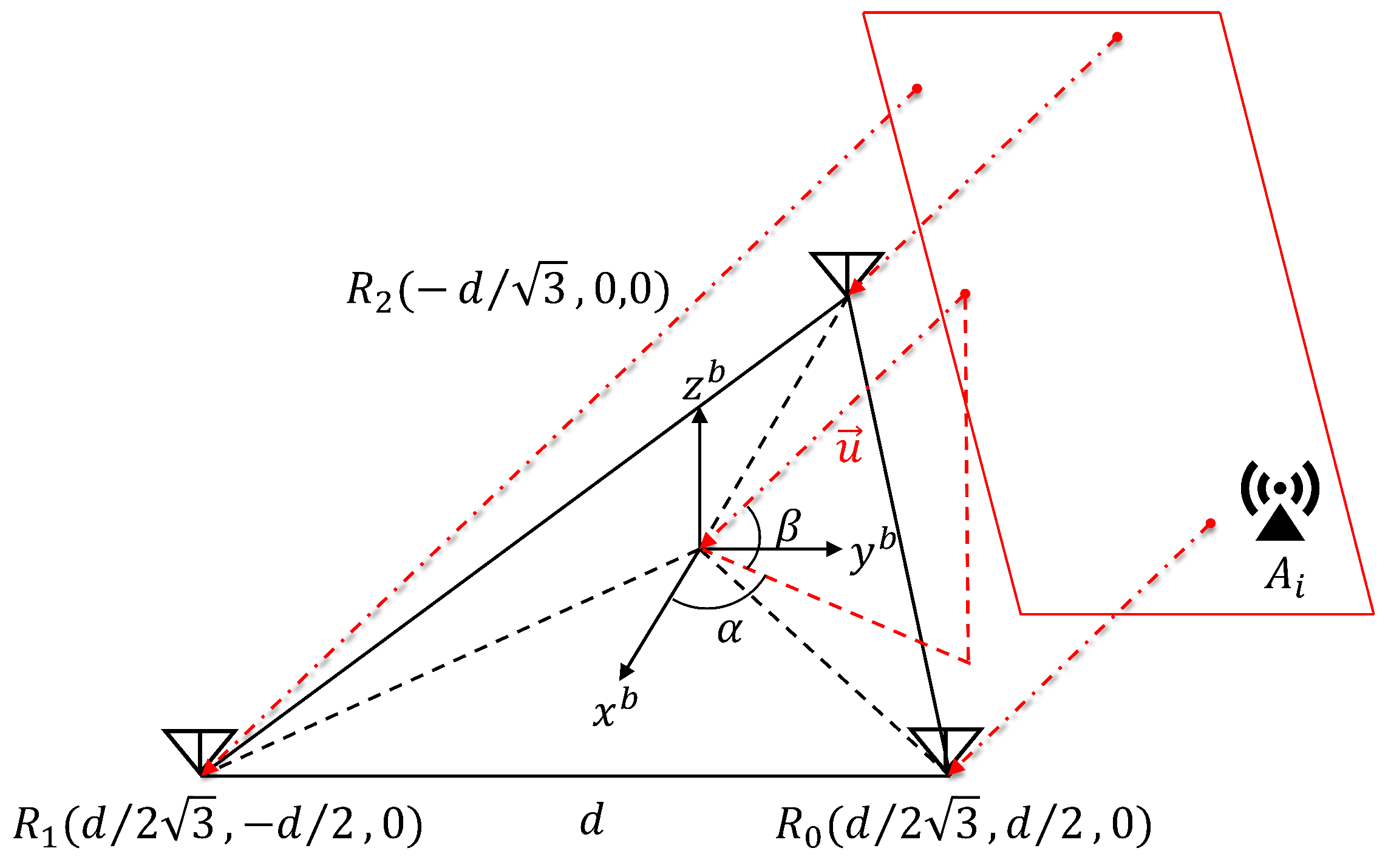
• A TC–ESKF–based UWB/IMU fusion framework is proposed. An antenna array is deployed on the UAV to obtain AOA measurements by processing phase differences of arrival (PDOA). For the first time, TDOA and AOA measurements from the UWB tag are jointly used to correct IMU propagation errors, enabling high-accuracy estimation of the full 6-DoF UAV pose.
• A weighted nonlinear least squares (WNLS)–based initialization algorithm is designed. Without relying on magnetometers, the algorithm fuses accelerometer measurements during the static phase with UWB measurements to rapidly estimate the UAV’s initial position and attitude. The estimated state serves as a precise and reliable initial value for ESKF, significantly improving the filter’s convergence rate and estimation stability.
• Simulation and real-world flight experiments are conducted, covering both static initialization and dynamic navigation stages. The proposed system is systematically evaluated under various flight conditions. Comparative results against several representative fusion algorithms demonstrate superior 3D position and yaw angle estimation performance.

The remainder of this paper is organized as follows. Section 2 presents the overall architecture and workflow of the proposed UWB/IMU-based localization system. Section 3 describes the static initialization algorithm and the TC–ESKF–based integrated navigation algorithm. Section 4 verifies the proposed system’s effectiveness and robustness through simulation and real flight experiments. Finally, Section 5 concludes the paper by summarizing the main findings.

2. Overview of the UWB/IMU-Based Localization System

In this section, the overall architecture of the proposed integrated navigation system is first introduced, followed by definitions of the adopted coordinate systems and descriptions of sensor measurements.

2.1. System Architecture

The proposed system is built on a lightweight UAV platform designed for high-precision position and attitude estimation in indoor GNSS-denied environments. It features strong scalability and supports simultaneous localization and attitude determination for multiple UAVs. Each UAV is equipped with an IMU and a UWB tag and runs the proposed fusion algorithm to achieve a 6-DoF state estimation. The structure of the proposed UAV localization system is illustrated in Figure 1, which presents a representative layout of the UWB positioning system.

The UWB positioning system consists of fixed anchors with known positions and mobile tags to be localized. In the system, five UWB anchors are deployed as reference nodes. Each UAV is equipped with a UWB tag that receives signals from the anchors and acquires measurement data. Both the anchors and tags use the HY-BI302 module, as shown in Figure 2. This module complies with the IEEE 802.15.4z standard, integrates an antenna array, and supports both ranging and PDOA measurements. The measurement data are transmitted to the onboard computing unit via a serial interface. The main parameters of the HY-BI302 UWB module used in this system are listed in

Table 1. Parameters of the UWB module.

Parameter	Unit	Value
Carrier frequency	MHz	6489.6
Bandwidth	MHz	499.2
Channel	–	5
Preamble length	Symbols	128
Preamble code type	–	9
Start-of-frame delimiter length	Symbols	8
Data rate	Mbps	6.81
Propagation distance	m	100

.

In addition to the UWB transceiver, the HY-BI302 module also integrates an ICM-40607 IMU, which includes a triaxial accelerometer and a triaxial gyroscope. It provides acceleration and angular velocity measurements in the body coordinate frame. The IMU data are also transmitted via serial interface and are fused with UWB measurements for state estimation. A summary of the key parameters of the ICM-40607 IMU is provided in

Table 2. Parameters of the ICM-40607 IMU.

Parameter	Unit	Value
Accelerometer range	g	±16
Accelerometer noise spectral density	µg$/\sqrt{\mathrm{Hz}}$	110
Accelerometer cross-axis sensitivity	%	±2
Accelerometer output data rate	Hz	1.5625–8000
Gyroscope range	$\mathrm{deg}$/s	±2000
Gyroscope noise spectral density	$\mathrm{deg}$/s/$\sqrt{\mathrm{Hz}}$	0.007
Gyroscope cross-axis sensitivity	%	±2
Gyroscope output data rate	Hz	12.5–8000

.

As shown in Figure 3, the UAV platform is a custom-built quadrotor developed in our laboratory. A UWB tag is mounted at the rear of the platform and connected to the onboard computer via a serial interface. The onboard computer collects data from sensors and the motion capture system, executes the proposed localization algorithm in real time, and records both raw measurements and estimated localization results.

2.2. Coordinate Systems

To accurately represent the UAV’s attitude and motion, two coordinate frames are defined: the navigation frame (denoted $\mathbf{n}$ frame) and the body frame (denoted $\mathbf{b}$ frame), as illustrated in Figure 1. The $\mathbf{n}$ adopts the East-North-Up (ENU) convention, with its origin located at a designated reference point in the experimental environment. The $x^n$, $y^n$, and $z^n$ axes point eastward, northward, and upward, respectively, forming a right-handed coordinate system. All state variables in the proposed algorithm are defined and estimated in the $\mathbf{n}$ frame. The $\mathbf{b}$ frame is defined with its $x^b$, $y^b$, and $z^b$ axes pointing to the right, forward, and upward directions of the UAV, respectively. The IMU is aligned with the $\mathbf{b}$ frame, and its measured accelerations and angular velocities are expressed in this frame. A Z–X–Y Euler angle sequence is adopted to describe the rotational relationship between the $\mathbf{b}$ and $\mathbf{n}$ frames. Let the UAV’s attitude be represented by the Euler angle triplet $\mathit{\theta }={[\varphi ,\theta ,\psi ]}^{\top }$, representing successive rotations about the $\mathbf{n}$-frame z axis (yaw $\psi$), x axis (pitch $\theta$), and y axis (roll $\varphi$). The direction cosine matrix ${\mathbf{C}}_n^b\left(\mathit{\theta }\right)$, which describes the transformation from the $\mathbf{n}$ frame to the $\mathbf{b}$ frame, is given by

$${\mathbf{C}}_n^b\left(\mathit{\theta }\right)={\mathbf{C}}_{\varphi }·{\mathbf{C}}_{\theta }·{\mathbf{C}}_{\psi }$$

(1)

$${\mathbf{C}}_{\varphi }=\left[\begin{array}{ccc}cos\varphi & 0& -sin\varphi \\ 0& 1& 0\\ sin\varphi & 0& cos\varphi \end{array}\right]$$

(2)

$${\mathbf{C}}_{\theta }=\left[\begin{array}{ccc}1& 0& 0\\ 0& cos\theta & sin\theta \\ 0& -sin\theta & cos\theta \end{array}\right]$$

(3)

$${\mathbf{C}}_{\psi }=\left[\begin{array}{ccc}cos\psi & sin\psi & 0\\ -sin\psi & cos\psi & 0\\ 0& 0& 1\end{array}\right]$$

(4)

2.3. UWB Measurements

The UWB positioning system adopts a downlink TDOA scheme in which multiple static anchors periodically broadcast ranging frames. At the same time, the onboard tag passively receives the signals and estimates the range differences relative to anchor pairs by comparing the received timestamps. Under the TDOA scheme, the tag only needs to receive signals passively, eliminating the requirement for precise clock synchronization with the anchors. The proposed system offers high capacity, low power consumption, and enhanced scalability.

To establish the TDOA measurement model, consider a system with M anchors, where the position of the i-th anchor $A_i$ is denoted ${\mathbf{p}}_i={[x_i,y_i,z_i]}^{\top }$. The position of the UAV in the navigation frame $\mathbf{n}$ is denoted $\mathbf{p}={[x,y,z]}^{\top }$. By comparing the TOA of signals from a reference anchor $A_0$ and a target anchor $A_i$, the tag obtains the distance difference to this anchor pair. The corresponding ideal measurement function of this range difference is defined as follows:

$$h_i^{\mathrm{tdoa}}\left(\mathbf{p}\right)=\parallel \mathbf{p}-{\mathbf{p}}_i\parallel -\parallel \mathbf{p}-{\mathbf{p}}_0\parallel$$

(5)

Considering the effect of measurement noise, the actual TDOA measurement is modeled as a noisy measurement:

$$z_i^{\mathrm{tdoa}}=h_i^{\mathrm{tdoa}}\left(\mathbf{p}\right)+n_i^{\mathrm{tdoa}},n_i^{\mathrm{tdoa}}\sim \mathcal{N}(0,{\sigma }_{\mathrm{tdoa}}^2)$$

(6)

Figure 4 shows that the UWB tag integrates three antennas, denoted $R_0$, $R_1$, and $R_2$, forming an equilateral triangular array. The array plane is aligned with the $\mathbf{b}$ frame, and its center is used as the reference point for angle estimation. The antenna spacing is set to $d=\lambda /2$, where $\lambda$ is the carrier wavelength of the UWB signal.

Under the far-field assumption, the wavefront of the UWB signal emitted from the anchor can be approximated as a plane wave. When the signal arrives at the antenna array, phase differences arise among the received signals due to the spatial separation between the antenna elements. By measuring the PDOA between the reference antenna, $R_0$, and antennas $R_1$ and $R_2$, the direction of arrival in the array plane can be estimated, enabling estimation of the signal’s AOA. Let $\alpha$ and $\beta$ denote the azimuth and elevation angles of the incoming signal, respectively. The unit vector representing the propagation direction of the signal transmitted by anchor $A_i$ in the $\mathbf{b}$ frame can be written as follows:

$$\mathbf{u}=-\left[\begin{array}{c}cos\beta cos\alpha \\ cos\beta sin\alpha \\ sin\beta \end{array}\right]$$

(7)

According to the single-frequency plane wave model, the PDOA is determined by the projected length of the displacement vector between the antenna pairs onto the direction of signal propagation. Let ${\mathbf{r}}_{R_i}$ denote the position of antenna $R_i$; then, the PDOA between the reference antenna $R_0$ and any antenna $R_i$ can be expressed as follows:

$$\mathrm{\Delta }{\phi }_{R_0,R_i}=-{\displaystyle \frac{2\pi }{\lambda }}·{\mathbf{u}}^{\top }({\mathbf{r}}_{R_i}-{\mathbf{r}}_{R_0})$$

(8)

Based on the geometric configuration shown in Figure 4, the PDOA between $R_0$ and $R_1$, $R_2$ can be further derived as follows:

$$\begin{array}{cc}\mathrm{\Delta }{\phi }_{R_0,R_1}\hfill & =-{\displaystyle \frac{2\pi d}{\lambda }}·cos\beta ·sin\alpha \hfill \end{array}$$

(9)

$$\begin{array}{cc}\mathrm{\Delta }{\phi }_{R_0,R_2}\hfill & =-{\displaystyle \frac{2\pi d}{\lambda }}·cos\beta ·\left({\displaystyle \frac{\sqrt{3}}{2}}cos\alpha +{\displaystyle \frac{1}{2}}sin\alpha \right)\hfill \end{array}$$

(10)

Based on Equations (9) and (10), $\alpha$ can be expressed as a function of the PDOA measurements:

$$\alpha =\mathrm{atan}2\left(-\sqrt{3}·\mathrm{\Delta }{\phi }_{R_0,R_1},-(2\mathrm{\Delta }{\phi }_{R_0,R_2}-\mathrm{\Delta }{\phi }_{R_0,R_1})\right)$$

(11)

Let the direction vector of anchor $A_i$ in the $\mathbf{b}$ frame be represented as

$$\begin{array}{c}{\mathbf{d}}_i^b={[d_{ix}^b,d_{iy}^b,d_{iz}^b]}^{\top }\hfill \end{array}$$

(12)

Its projection onto the $x^b$–$y^b$ plane corresponds to the azimuth angle of the incoming signal, which is considered the ground truth AOA measurement in this work. Only the azimuth angle is used, and elevation angle estimation is not included. The ground truth AOA measurement is defined as follows:

$$\begin{array}{cc}\hfill & {\mathbf{d}}_i^b={\mathbf{C}}_n^b\left(\mathit{\theta }\right)({\mathbf{p}}_i-\mathbf{p})\hfill \end{array}$$

(13)

$$\begin{array}{cc}\hfill & h_i^{\mathrm{aoa}}(\mathbf{p},\mathit{\theta })=\mathrm{atan}2(d_{iy}^b,d_{ix}^b)\hfill \end{array}$$

(14)

The actual AOA measurement, denoted $z_i^{\mathrm{aoa}}$, is estimated from the PDOA measured by the antenna array using Equation (11) and is subject to measurement noise. The measurement model is expressed as follows:

$$z_i^{\mathrm{aoa}}=h_i^{\mathrm{aoa}}(\mathbf{p},\mathit{\theta })+n_i^{\mathrm{aoa}},n_i^{\mathrm{aoa}}\sim \mathcal{N}(0,{\sigma }_{\mathrm{aoa}}^2)$$

(15)

2.4. Workflow of the Proposed System

Figure 5 illustrates the workflow of the proposed localization system. The system integrates two types of sensors: the IMU provides high-frequency measurements of specific force and angular velocity for state prediction, while the UWB tag receives signals from multiple anchors at a lower rate to obtain TDOA and AOA measurements for error-state correction. During the initial static phase following system startup, a short time window of multi-source measurements is utilized to estimate the UAV’s initial position and attitude using a WNLS approach. Once initialization is complete, the system enters a recursive loop, where IMU data drives the prediction of the nominal state, and incoming UWB measurements trigger the update of the error state. The entire estimation framework is based on a TC-ESKF, which continuously outputs the 6-DoF state of the UAV, including both position and attitude.

3. Proposed State Estimation Algorithm

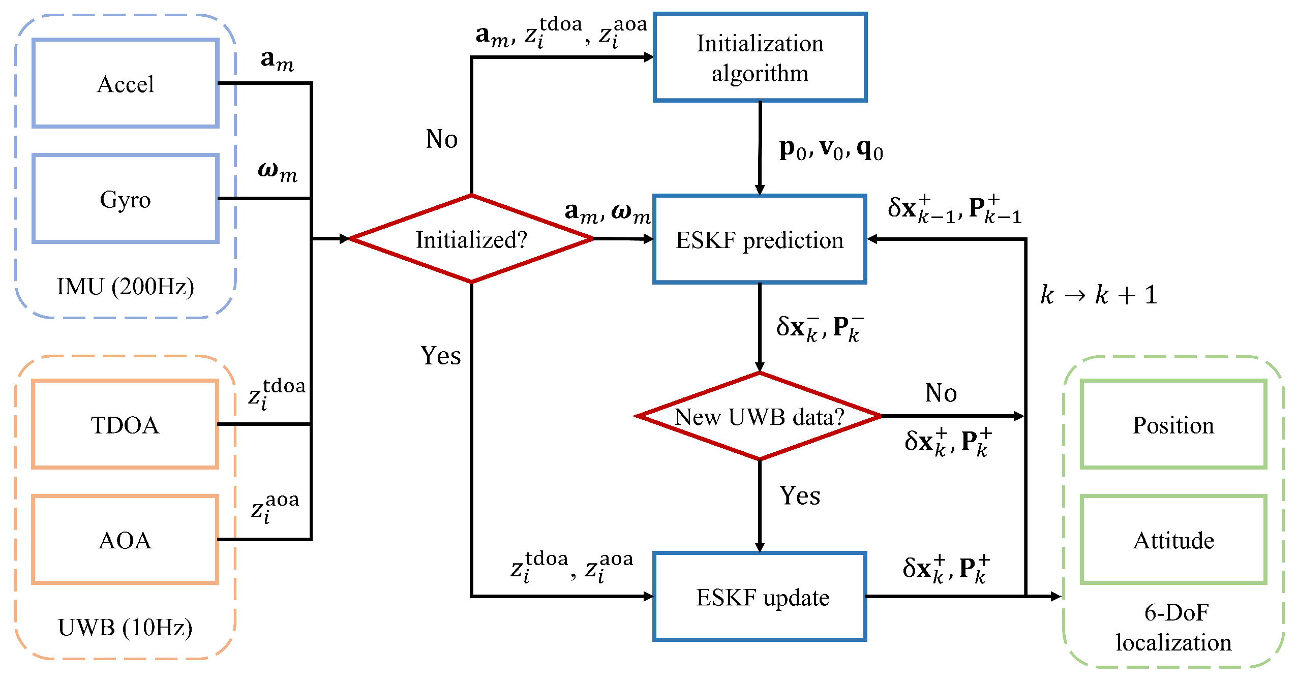
This paper proposes a state estimation framework based on IMU and UWB data to achieve high-precision navigation in indoor environments. The framework consists of two main components: an initialization algorithm during the static phase and a sensor fusion algorithm for the flight phase. Using a WNLS algorithm, the system estimates the UAV’s initial position and attitude in the initialization phase. This estimation integrates the specific force measurements provided by the IMU and the averaged static measurements from the UWB system. The resulting estimate serves as the initial state of the filter. During the flight phase, the system performs tightly coupled fusion of the IMU dynamic data with the raw TDOA and AOA measurements from the UWB tag using the ESKF algorithm, enabling continuous estimation of position and attitude.

During the initialization phase, the UAV remains static. The acceleration measured by the IMU can be regarded as the negative projection of gravitational acceleration in the $\mathbf{b}$ frame. Let ${\overline{\mathbf{a}}}^b={[{\overline{a}}_x^b,{\overline{a}}_y^b,{\overline{a}}_z^b]}^{\top }$ denote the average triaxial acceleration measured by the IMU over a 1-second static window. The pitch and roll angles of the UAV can then be estimated according to Equations (16) and (17) [31]:

$$\begin{array}{cc}\theta \hfill & =arcsin\left({\displaystyle \frac{{\overline{a}}_y^b}{\sqrt{{\left({\overline{a}}_x^b\right)}^2+{\left({\overline{a}}_y^b\right)}^2+{\left({\overline{a}}_z^b\right)}^2}}}\right)\hfill \end{array}$$

(16)

$$\begin{array}{cc}\varphi \hfill & =arcsin\left(-{\displaystyle \frac{{\overline{a}}_x^b}{\sqrt{{\left({\overline{a}}_x^b\right)}^2+{\left({\overline{a}}_y^b\right)}^2+{\left({\overline{a}}_z^b\right)}^2}·cos\theta }}\right)\hfill \end{array}$$

(17)

Due to the high noise level of gyroscopes in low-cost MEMS inertial sensors, the angular velocity caused by Earth’s rotation is difficult to detect in a static state. Therefore, yaw angle estimation based solely on gyroscope measurements is unreliable. To address this, after initializing the pitch and roll angles, the system employs a WNLS algorithm to jointly estimate the UAV’s 3D position and yaw angle using the averaged TDOA and AOA measurements collected over the same 1-second static window.

The variable to be optimized is denoted $\xi ={[x,y,z,\psi ]}^{\top }$. Based on the initialized pitch and roll angles, the residual functions for TDOA and AOA are constructed as follows, where $wrap(·)$ denotes the angle normalization operation that maps values to the interval $[-\pi ,\pi )$.

$$\begin{array}{c}{r}_i^{\mathrm{tdoa}}={\displaystyle \frac{1}{{\sigma }_{\mathrm{tdoa}}}}(z_i^{\mathrm{tdoa}}-\left(\parallel \mathbf{p}-{\mathbf{p}}_i\parallel -\parallel \mathbf{p}-{\mathbf{p}}_0\parallel \right)),i=1,\dots ,M-1\hfill \end{array}$$

(18)

$$\begin{array}{c}{r}_i^{\mathrm{aoa}}={\displaystyle \frac{1}{{\sigma }_{\mathrm{aoa}}}}\left(\mathrm{wrap}(z_i^{\mathrm{aoa}}-\mathrm{atan}2(d_{iy}^b,d_{ix}^b))\right),i=0,\dots ,M-1\hfill \end{array}$$

(19)

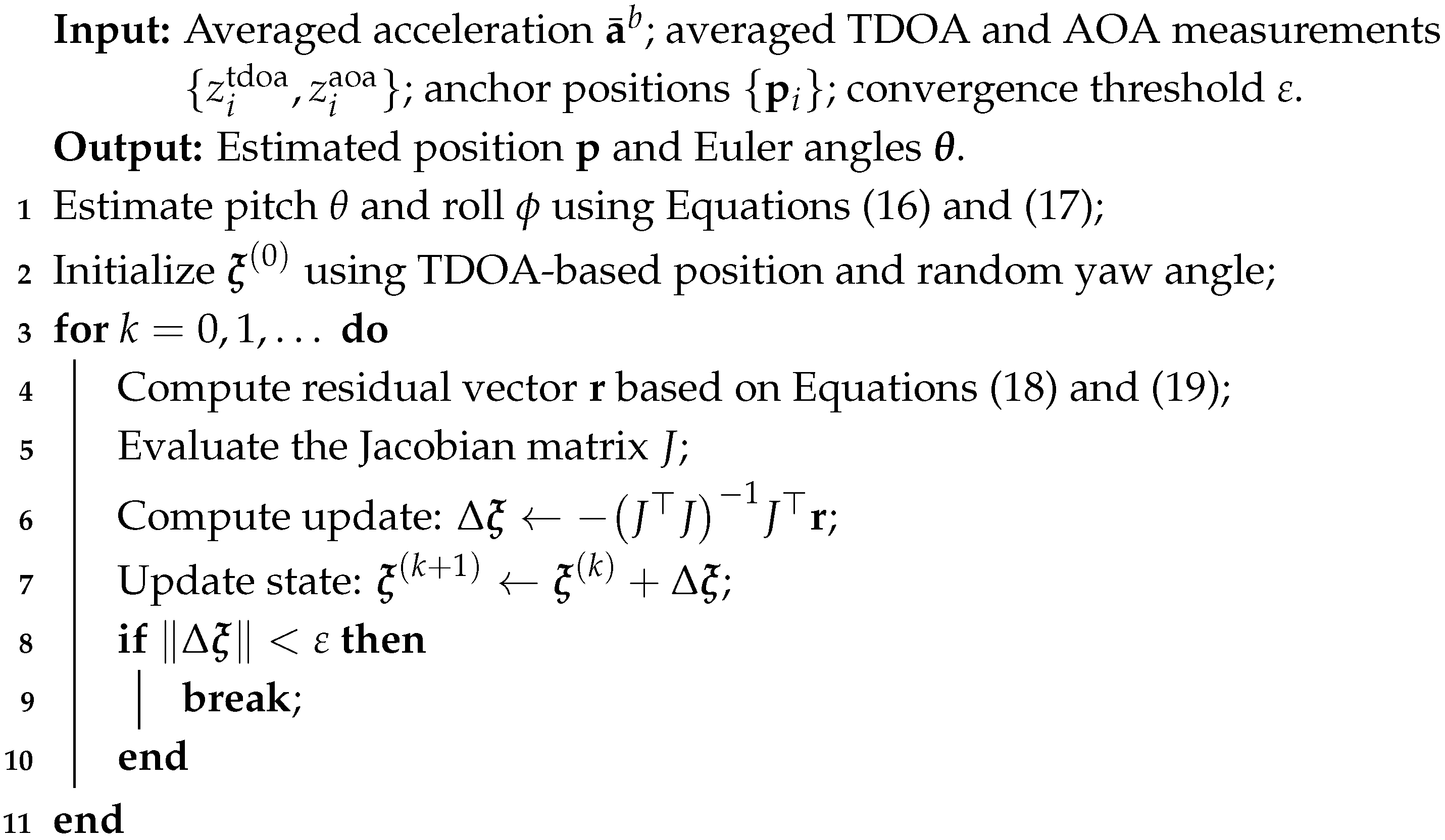
The corresponding WNLS cost function is defined in Equation (20), and the optimization is carried out using the Gauss–Newton method to iteratively solve for $\xi$. In this process, the stacked residual vector $\mathbf{r}$ and the Jacobian matrix $\mathbf{J}$ are defined in Equations (21) and (22), respectively. A complete summary of the initialization process is provided in Algorithm 1.

$$\mathcal{L}\left(\xi \right)=\sum _{i=1}^{M-1}{\left(r_i^{\mathrm{tdoa}}\right)}^2+\sum _{i=0}^{M-1}{\left(r_i^{\mathrm{aoa}}\right)}^2$$

(20)

$$\mathbf{r}={\left[r_1^{\mathrm{tdoa}},\dots ,r_{M-1}^{\mathrm{tdoa}},r_0^{\mathrm{aoa}},\dots ,r_M^{\mathrm{aoa}}\right]}^{\top }\in {\mathbb{R}}^{(2M-1)\times 1}$$

(21)

$$\mathbf{J}={\displaystyle \frac{\partial \mathbf{r}}{\partial \xi }}={({\displaystyle \frac{\partial \mathbf{r}}{\partial x}},{\displaystyle \frac{\partial \mathbf{r}}{\partial y}},{\displaystyle \frac{\partial \mathbf{r}}{\partial z}},{\displaystyle \frac{\partial \mathbf{r}}{\partial \psi }})}^{\top }\in {\mathbb{R}}^{(2M-1)\times 4}$$

(22)

Although the UWB system can provide position measurements of the UAV, complete attitude information is typically not directly available during flight. However, attitude awareness is crucial for ensuring stable UAV control. To address this, this paper proposes a fusion algorithm based on TC–ESKF, which directly fuses the raw measurements from the UWB system with IMU outputs to achieve continuous estimation of the UAV’s 6-DoF state. The proposed algorithm demonstrates greater robustness and estimation stability than conventional loosely coupled algorithms, particularly under degraded measurement conditions or increased measurement noise. Unit quaternions are adopted to represent UAV attitude to avoid singularities and enhance numerical stability.

Algorithm 1: Proposed initialization algorithm for position and attitude.

The system state includes the UAV’s 3D position $\mathbf{p}$ and velocity $\mathbf{v}$, both expressed in the $\mathbf{n}$ frame, as well as the attitude quaternion ${\mathbf{q}}_b^n$, the accelerometer bias ${\mathbf{b}}_a$, and the gyroscope bias ${\mathbf{b}}_g$. The ESKF divides the state variables into three categories: the true state ${\mathbf{x}}_t$, the nominal state $\mathbf{x}$, and the error state $\delta \mathbf{x}$. The nominal state describes the nonlinear motion evolution of the system and is propagated using IMU data during the prediction phase. In contrast, the error state represents the deviation of the nominal state from the true state and is used to correct the state during the update phase. The definitions of the nominal and error states are as follows:

$$\begin{array}{cc}\mathbf{x}\hfill & ={\left[\begin{array}{ccccc}{\mathbf{p}}^{\top }& {\mathbf{v}}^{\top }& {\mathbf{q}}^{\top }& {\mathbf{b}}_a^{\top }& {\mathbf{b}}_g^{\top }\end{array}\right]}^{\top }\in {\mathbb{R}}^{16}\hfill \end{array}$$

(23)

$$\begin{array}{cc}\delta \mathbf{x}\hfill & ={\left[\begin{array}{ccccc}\delta {\mathbf{p}}^{\top }& \delta {\mathbf{v}}^{\top }& \delta {\mathit{\theta }}^{\top }& \delta {\mathbf{b}}_a^{\top }& \delta {\mathbf{b}}_g^{\top }\end{array}\right]}^{\top }\in {\mathbb{R}}^{15}\hfill \end{array}$$

(24)

To avoid potential redundancy and normalization constraints associated with error quaternion representations and to enhance computational efficiency, the attitude error is modeled as a three-dimensional Euler angle error $\delta \mathit{\theta }$. This vector is then converted into the error quaternion $\delta \mathbf{q}$, which is applied to correct the nominal quaternion state. The first-order approximation of $\delta \mathbf{q}$ is given by $\delta \mathbf{q}\approx {[1,{(\delta \mathit{\theta }/2)}^{\top }]}^{\top }$. The true state is then reconstructed by combining the nominal and error states through either linear or nonlinear operations, as detailed below, where ⊗ denotes the quaternion multiplication operator.

$$\begin{array}{c}{\mathbf{x}}_t=\left[\begin{array}{c}{\mathbf{p}}_t\\ {\mathbf{v}}_t\\ {\mathbf{q}}_t\\ {\mathbf{b}}_{a,t}\\ {\mathbf{b}}_{g,t}\end{array}\right]=\left[\begin{array}{c}\mathbf{p}+\delta \mathbf{p}\\ \mathbf{v}+\delta \mathbf{v}\\ \mathbf{q}\otimes \delta \mathbf{q}\\ {\mathbf{b}}_a+\delta {\mathbf{b}}_a\\ {\mathbf{b}}_g+\delta {\mathbf{b}}_g\end{array}\right]\in {\mathbb{R}}^{16\times 1}\hfill \end{array}$$

(25)

The IMU provides measurements of specific force and angular velocity through the accelerometer and gyroscope, respectively. However, these measurements are typically affected by bias and random noise. In this work, the measurement noise is modeled as zero-mean Gaussian white noise, while the bias is modeled as a random walk process driven by white noise. The corresponding model is given in Equation (26), where ${\mathbf{n}}_{ba}\sim \mathcal{N}(0,{\sigma }_{ba}^2·{\mathbf{I}}_{\mathbf{3}\times \mathbf{3}})$ and ${\mathbf{n}}_{bg}\sim \mathcal{N}(0,{\sigma }_{bg}^2·{\mathbf{I}}_{\mathbf{3}\times \mathbf{3}})$.

$$\begin{array}{c}{\dot{\mathbf{b}}}_a={\mathbf{n}}_{ba},{\dot{\mathbf{b}}}_g={\mathbf{n}}_{bg}\hfill \end{array}$$

(26)

Based on the accelerometer and gyroscope measurements, denoted ${\mathbf{a}}_m$ and ${\omega }_m$, the angular velocity and acceleration of the UAV in the $\mathbf{n}$ frame can be computed, as shown in Equation (27). Here, $\mathbf{C}\left({\mathbf{q}}_b^n\right)$ denotes the direction cosine matrix converted from the quaternion ${\mathbf{q}}_b^n$. The terms ${\mathbf{n}}_a\sim \mathcal{N}(0,{\sigma }_a^2·{\mathbf{I}}_{\mathbf{3}\times \mathbf{3}})$ and ${\mathbf{n}}_g\sim \mathcal{N}(0,{\sigma }_g^2·{\mathbf{I}}_{\mathbf{3}\times \mathbf{3}})$ represent the zero-mean Gaussian noise associated with the accelerometer and gyroscope measurements, respectively.

$$\begin{array}{c}\omega ={\omega }_m-{\mathbf{b}}_g-{\mathbf{n}}_g,\mathbf{a}=\mathbf{C}\left({\mathbf{q}}_b^n\right)({\mathbf{a}}_m-{\mathbf{b}}_a-{\mathbf{n}}_a)+\mathbf{g}\hfill \end{array}$$

(27)

Whenever new IMU measurements become available, the filter recursively updates the nominal state based on these measurements. The kinematic equations of the nominal state in continuous time are given in Equation (28):

$$\begin{array}{c}\dot{\mathbf{x}}=\left[\begin{array}{c}\dot{\mathbf{p}}\\ \dot{\mathbf{v}}\\ \dot{\mathbf{q}}\\ {\dot{\mathbf{b}}}_a\\ {\dot{\mathbf{b}}}_g\end{array}\right]=\left[\begin{array}{c}\mathbf{v}\\ \mathbf{C}\left({\mathbf{q}}_b^n\right)({\mathbf{a}}_m-{\mathbf{b}}_a)+\mathbf{g}\\ {\displaystyle \frac{1}{2}}\mathbf{q}\otimes ({\omega }_m-{\mathbf{b}}_g)\\ \mathbf{0}\\ \mathbf{0}\end{array}\right]\hfill \end{array}$$

(28)

The true state and nominal state share the same kinematic model, with the main difference being that the true state includes sensor noise terms. Based on a linearization approach, the continuous-time propagation model of the error state is formulated as follows:

$$\begin{array}{c}\dot{\delta \mathbf{x}}=\left[\begin{array}{c}\dot{\delta \mathbf{p}}\\ \dot{\delta \mathbf{v}}\\ \dot{\delta \mathit{\theta }}\\ {\dot{\delta \mathbf{b}}}_a\\ {\dot{\delta \mathbf{b}}}_g\end{array}\right]=\left[\begin{array}{c}\delta \mathbf{v}\\ -\mathbf{C}\left({\mathbf{q}}_b^n\right){\left[{\mathbf{a}}_m-{\mathbf{b}}_a\right]}_{\times }\delta \mathit{\theta }-\mathbf{C}\left({\mathbf{q}}_b^n\right)\delta {\mathbf{b}}_a-\mathbf{C}\left({\mathbf{q}}_b^n\right){\mathbf{n}}_a\\ -{\left[{\omega }_m-{\mathbf{b}}_g\right]}_{\times }\delta \mathit{\theta }-\delta {\mathbf{b}}_g-{\mathbf{n}}_g\\ {\mathbf{n}}_{ba}\\ {\mathbf{n}}_{bg}\end{array}\right]\hfill \end{array}$$

(29)

The state propagation process includes the recursive update of the error state and the propagation of the covariance matrix. In discrete time, the kinematic equation of the error state can be expressed as follows:

$$\begin{array}{cc}\delta {\mathbf{x}}_{k+1}\hfill & =\left[\begin{array}{c}\delta {\mathbf{p}}_{k+1}\\ \delta {\mathbf{v}}_{k+1}\\ \delta {\mathit{\theta }}_{k+1}\\ \delta {\mathbf{b}}_{a,k+1}\\ \delta {\mathbf{b}}_{g,k+1}\end{array}\right]\hfill \\ \hfill & =\left[\begin{array}{c}\delta {\mathbf{p}}_k+\delta {\mathbf{v}}_k\mathrm{\Delta }t\\ \delta {\mathbf{v}}_k+\left(-\mathbf{C}\left({\mathbf{q}}_{b,k}^n\right){\left[{\mathbf{a}}_{m,k}-{\mathbf{b}}_{a,k}\right]}_{\times }\delta {\mathit{\theta }}_k-\mathbf{C}\left({\mathbf{q}}_{b,k}^n\right)\delta {\mathbf{b}}_{a,k}\right)\mathrm{\Delta }t+{\mathbf{n}}_{v,k}\\ \mathbf{C}{\left({\mathbf{q}}_{b,k}^n\right)}^{\top }\left\{({\omega }_{m,k}-{\mathbf{b}}_{g,k})\mathrm{\Delta }t\right\}\delta {\mathit{\theta }}_k-\delta {\mathbf{b}}_{g,k}\mathrm{\Delta }t+{\mathbf{n}}_{\omega ,k}\\ \delta {\mathbf{b}}_{a,k}+{\mathbf{n}}_{ba,k}\\ \delta {\mathbf{b}}_{g,k}+{\mathbf{n}}_{bg,k}\end{array}\right]\hfill \end{array}$$

(30)

The covariance matrices of the noise terms are defined as follows:

$$\begin{array}{cc}\mathbb{E}\left[{\mathbf{n}}_{v,k}{\mathbf{n}}_{v,k}^{\top }\right]\hfill & ={\sigma }_a^2\mathrm{\Delta }t·{\mathbf{I}}_{3\times 3}\hfill \end{array}$$

(31)

$$\begin{array}{cc}\mathbb{E}\left[{\mathbf{n}}_{\omega ,k}{\mathbf{n}}_{\omega ,k}^{\top }\right]\hfill & ={\sigma }_g^2\mathrm{\Delta }t·{\mathbf{I}}_{3\times 3}\hfill \end{array}$$

(32)

$$\begin{array}{cc}\mathbb{E}\left[{\mathbf{n}}_{ba,k}{\mathbf{n}}_{ba,k}^{\top }\right]\hfill & ={\sigma }_{ba}^2\mathrm{\Delta }t·{\mathbf{I}}_{3\times 3}\hfill \end{array}$$

(33)

$$\begin{array}{cc}\mathbb{E}\left[{\mathbf{n}}_{bg,k}{\mathbf{n}}_{bg,k}^{\top }\right]\hfill & ={\sigma }_{bg}^2\mathrm{\Delta }t·{\mathbf{I}}_{3\times 3}\hfill \end{array}$$

(34)

Equations (35) and (36) summarize the discrete-time propagation form of the error state and its covariance matrix. Here, ${\mathbf{F}}_k$, ${\mathbf{G}}_k$, ${\mathbf{w}}_k$, and ${\mathbf{Q}}_k$ denote the error-state transition matrix, process noise mapping matrix, process noise vector, and its covariance matrix, respectively. Their specific structures are provided in Equations (37)–(40).

$$\begin{array}{cc}\delta {\mathbf{x}}_{k+1}^{-}\hfill & ={\mathbf{F}}_k\delta {\mathbf{x}}_k^{+}+{\mathbf{G}}_k{\mathbf{w}}_k\hfill \end{array}$$

(35)

$$\begin{array}{cc}{\mathbf{P}}_{k+1}^{-}\hfill & ={\mathbf{F}}_k{\mathbf{P}}_k^{+}{\mathbf{F}}_k^{\top }+{\mathbf{G}}_k{\mathbf{Q}}_k{\mathbf{G}}_k^{\top }\hfill \end{array}$$

(36)

$$\begin{array}{cc}{\mathbf{F}}_k\hfill & =\left[\begin{array}{ccccc}{\mathbf{I}}_{3\times 3}& \mathrm{\Delta }t·{\mathbf{I}}_{3\times 3}& \mathbf{0}& \mathbf{0}& \mathbf{0}\\ \mathbf{0}& {\mathbf{I}}_{3\times 3}& -\mathbf{C}\left({\mathbf{q}}_{b,k}^n\right){\left[{\mathbf{a}}_{m,k}-{\mathbf{b}}_{a,k}\right]}_{\times }\mathrm{\Delta }t& -\mathbf{C}\left({\mathbf{q}}_{b,k}^n\right)\mathrm{\Delta }t& \mathbf{0}\\ \mathbf{0}& \mathbf{0}& \mathbf{C}{\left({\mathbf{q}}_{b,k}^n\right)}^{\top }\left\{({\omega }_{m,k}-{\mathbf{b}}_{g,k})\mathrm{\Delta }t\right\}& \mathbf{0}& -\mathrm{\Delta }t·{\mathbf{I}}_{3\times 3}\\ \mathbf{0}& \mathbf{0}& \mathbf{0}& {\mathbf{I}}_{3\times 3}& \mathbf{0}\\ \mathbf{0}& \mathbf{0}& \mathbf{0}& \mathbf{0}& {\mathbf{I}}_{3\times 3}\end{array}\right]\hfill \end{array}$$

(37)

$$\begin{array}{cc}{\mathbf{G}}_k\hfill & =\left[\begin{array}{cccc}\mathbf{0}& \mathbf{0}& \mathbf{0}& \mathbf{0}\\ {\mathbf{I}}_{3\times 3}& \mathbf{0}& \mathbf{0}& \mathbf{0}\\ \mathbf{0}& {\mathbf{I}}_{3\times 3}& \mathbf{0}& \mathbf{0}\\ \mathbf{0}& \mathbf{0}& {\mathbf{I}}_{3\times 3}& \mathbf{0}\\ \mathbf{0}& \mathbf{0}& \mathbf{0}& {\mathbf{I}}_{3\times 3}\end{array}\right]\hfill \end{array}$$

(38)

$$\begin{array}{cc}{\mathbf{w}}_k\hfill & =\left[\begin{array}{c}{\mathbf{n}}_{v,k}\\ {\mathbf{n}}_{\omega ,k}\\ {\mathbf{n}}_{ba,k}\\ {\mathbf{n}}_{bg,k}\end{array}\right]\hfill \end{array}$$

(39)

$$\begin{array}{cc}{\mathbf{Q}}_k\hfill & =\left[\begin{array}{cccc}{\sigma }_a^2\mathrm{\Delta }t·{\mathbf{I}}_{3\times 3}& \mathbf{0}& \mathbf{0}& \mathbf{0}\\ \mathbf{0}& {\sigma }_g^2\mathrm{\Delta }t·{\mathbf{I}}_{3\times 3}& \mathbf{0}& \mathbf{0}\\ \mathbf{0}& \mathbf{0}& {\sigma }_{ba}^2\mathrm{\Delta }t·{\mathbf{I}}_{3\times 3}& \mathbf{0}\\ \mathbf{0}& \mathbf{0}& \mathbf{0}& {\sigma }_{bg}^2\mathrm{\Delta }t·{\mathbf{I}}_{3\times 3}\end{array}\right]\hfill \end{array}$$

(40)

To suppress divergence caused by the accumulation of inertial errors, the system incorporates measurements from the UWB system on top of state propagation, correcting both the error state and its covariance matrix. Let $\mathbf{h}\left({\mathbf{x}}_t\right)$ denote the joint measurement function, composed of $M-1$ TDOA and M AOA measurements, where M denotes the number of anchors in the system. Its nonlinear measurement model is given by

$$\begin{array}{c}\mathbf{z}=\mathbf{h}\left({\mathbf{x}}_t\right)+\mathbf{v}=\left[\begin{array}{c}{h}_1^{\mathrm{tdoa}}\left({\mathbf{p}}_t\right)\\ ⋮\\ h_{M-1}^{\mathrm{tdoa}}\left({\mathbf{p}}_t\right)\\ h_0^{\mathrm{aoa}}({\mathbf{p}}_t,{\mathit{\theta }}_t)\\ ⋮\\ h_{M-1}^{\mathrm{aoa}}({\mathbf{p}}_t,{\mathit{\theta }}_t)\end{array}\right]+\left[\begin{array}{c}{n}_1^{\mathrm{tdoa}}\\ ⋮\\ n_{M-1}^{\mathrm{tdoa}}\\ n_0^{\mathrm{aoa}}\\ ⋮\\ n_{M-1}^{\mathrm{aoa}}\end{array}\right]\in {\mathbb{R}}^{(2M-1)\times 1}\hfill \end{array}$$

(41)

The vector $\mathbf{v}$ denotes the joint measurement noise, consisting of independently distributed, zero-mean TDOA and AOA measurement errors. Its covariance matrix is defined as follows:

$$\begin{array}{c}\mathbf{v}\sim \mathcal{N}\left(\mathbf{0},\mathbf{R}\right),\mathbf{R}=\left[\begin{array}{cc}{\sigma }_{\mathrm{tdoa}}^2·{\mathbf{I}}_{(M-1)\times (M-1)}& \mathbf{0}\\ \mathbf{0}& {\sigma }_{\mathrm{aoa}}^2·{\mathbf{I}}_{M\times M}\end{array}\right]\hfill \end{array}$$

(42)

To incorporate the nonlinear measurement function into the filter update step, it is necessary to linearize it with respect to the error state. The Jacobian of the joint measurement function with respect to the error state is denoted $\mathbf{H}=\partial \mathbf{h}/\partial \delta \mathbf{x}$. TDOA measurements are only related to the UAV’s position and are independent of its velocity, attitude, or IMU biases. Therefore, the derivative with respect to the error state has non-zero components only in the position error dimension $\delta \mathbf{p}$, while all other components are zero. According to the chain rule, we have

$$\begin{array}{c}{\displaystyle \frac{\partial h_i^{\mathrm{tdoa}}}{\partial \delta \mathbf{p}}}={\left.{\displaystyle \frac{\partial h_i^{\mathrm{tdoa}}}{\partial {\mathbf{p}}_t}}\phantom{{\displaystyle \frac{\partial {\mathbf{p}}_t}{\partial \delta \mathbf{p}}}}\right|}_{\mathbf{p}}·{\left.{\displaystyle \frac{\partial {\mathbf{p}}_t}{\partial \delta \mathbf{p}}}\phantom{{\displaystyle \frac{\partial h_i^{\mathrm{tdoa}}}{\partial {\mathbf{p}}_t}}}\right|}_{\mathbf{p}}={\left({\displaystyle \frac{\mathbf{p}-{\mathbf{p}}_i}{\parallel \mathbf{p}-{\mathbf{p}}_i\parallel }}-{\displaystyle \frac{\mathbf{p}-{\mathbf{p}}_0}{\parallel \mathbf{p}-{\mathbf{p}}_0\parallel }}\right)}^{\top }\hfill \end{array}$$

(43)

Thus, the Jacobian of $h_i^{\mathrm{tdoa}}$ with respect to the error state $\delta \mathbf{x}$ is given by

$$\begin{array}{c}{\mathbf{H}}_i^{\mathrm{tdoa}}=\left[\begin{array}{cc}{\left({\displaystyle \frac{\mathbf{p}-{\mathbf{p}}_i}{\parallel \mathbf{p}-{\mathbf{p}}_i\parallel }}-{\displaystyle \frac{\mathbf{p}-{\mathbf{p}}_0}{\parallel \mathbf{p}-{\mathbf{p}}_0\parallel }}\right)}^{\top }& {\mathbf{0}}_{1\times 12}\end{array}\right]\in {\mathbb{R}}^{1\times 15}\hfill \end{array}$$

(44)

Since AOA measurements depend on both the UAV’s position and attitude, their Jacobians with respect to the error state include non-zero components in $\delta \mathbf{p}$ and $\delta \mathit{\theta }$. The corresponding partial derivatives are as follows, where ${\left[{\mathbf{d}}_{\mathbf{i}}^{\mathbf{b}}\right]}_{\times }$ denotes the skew-symmetric matrix of ${\mathbf{d}}_{\mathbf{i}}^{\mathbf{b}}$:

$$\begin{array}{cc}{\displaystyle \frac{\partial h_i^{\mathrm{aoa}}}{\partial \delta \mathbf{p}}}\hfill & ={\left.{\displaystyle \frac{\partial h_i^{\mathrm{aoa}}}{\partial {\mathbf{d}}_i^b}}\right|}_{\mathbf{x}}·{\left.{\displaystyle \frac{\partial {\mathbf{d}}_i^b}{\partial \delta \mathbf{p}}}\right|}_{\mathbf{x}}\hfill \\ \hfill & ={\displaystyle \frac{1}{{\left(d_{ix}^b\right)}^2+{\left(d_{iy}^b\right)}^2}}\left[\begin{array}{ccc}-d_{iy}^b& d_{ix}^b& 0\end{array}\right]·{\displaystyle \frac{\partial \left({\mathbf{C}}_n^b\left(\mathit{\theta }\right)({\mathbf{p}}_i-\mathbf{p})\right)}{\partial \delta \mathbf{p}}}\hfill \\ \hfill & =-{\displaystyle \frac{1}{{\left(d_{ix}^b\right)}^2+{\left(d_{iy}^b\right)}^2}}\left[\begin{array}{ccc}-d_{iy}^b& d_{ix}^b& 0\end{array}\right]·{\mathbf{C}}_n^b\left(\mathit{\theta }\right)\hfill \end{array}$$

(45)

$$\begin{array}{cc}{\displaystyle \frac{\partial h_i^{\mathrm{aoa}}}{\partial \delta \mathit{\theta }}}\hfill & ={\left.{\displaystyle \frac{\partial h_i^{\mathrm{aoa}}}{\partial {\mathbf{d}}_i^b}}\right|}_{\mathbf{x}}·{\left.{\displaystyle \frac{\partial {\mathbf{d}}_i^b}{\partial \delta \mathit{\theta }}}\right|}_{\mathbf{x}}\hfill \\ \hfill & ={\displaystyle \frac{1}{{\left(d_{ix}^b\right)}^2+{\left(d_{iy}^b\right)}^2}}\left[\begin{array}{ccc}-d_{iy}^b& d_{ix}^b& 0\end{array}\right]·{\displaystyle \frac{\partial \left(\left(\mathbf{I}-{\left[\delta \mathit{\theta }\right]}_{\times }\right){\mathbf{C}}_n^b\left(\mathit{\theta }\right)({\mathbf{p}}_i-\mathbf{p})\right)}{\partial \delta \mathit{\theta }}}\hfill \\ \hfill & ={\displaystyle \frac{1}{{\left(d_{ix}^b\right)}^2+{\left(d_{iy}^b\right)}^2}}\left[\begin{array}{ccc}-d_{iy}^b& d_{ix}^b& 0\end{array}\right]·{\displaystyle \frac{\partial \left({\mathbf{d}}_i^b-{\left[\delta \mathit{\theta }\right]}_{\times }{\mathbf{d}}_i^b\right)}{\partial \delta \mathit{\theta }}}\hfill \\ \hfill & ={\displaystyle \frac{1}{{\left(d_{ix}^b\right)}^2+{\left(d_{iy}^b\right)}^2}}\left[\begin{array}{ccc}-d_{iy}^b& d_{ix}^b& 0\end{array}\right]·{\left[{\mathbf{d}}_i^b\right]}_{\times }\hfill \end{array}$$

(46)

Therefore, the Jacobian of $h_i^{\mathrm{aoa}}$ with respect to $\delta \mathbf{x}$ can be compactly written as follows:

$$\begin{array}{c}{\mathbf{H}}_i^{\mathrm{aoa}}={\displaystyle \frac{1}{{\left(d_{ix}^b\right)}^2+{\left(d_{iy}^b\right)}^2}}\left[\begin{array}{ccc}-d_{iy}^b& d_{ix}^b& 0\end{array}\right]·\left[\begin{array}{cccc}-{\mathbf{C}}_n^b\left(\mathit{\theta }\right)& {\mathbf{0}}_{3\times 3}& {\left[{\mathbf{d}}_i^b\right]}_{\times }& {\mathbf{0}}_{3\times 6}\end{array}\right]\in {\mathbb{R}}^{1\times 15}\hfill \end{array}$$

(47)

Based on Equations (44) and (47), the joint measurement matrix $\mathbf{H}$ is constructed as follows:

$$\begin{array}{c}\mathbf{H}={\left[{\left({\mathbf{H}}_1^{\mathrm{tdoa}}\right)}^{\top },\dots ,{\left({\mathbf{H}}_{M-1}^{\mathrm{tdoa}}\right)}^{\top },{\left({\mathbf{H}}_0^{\mathrm{aoa}}\right)}^{\top },\dots ,{\left({\mathbf{H}}_{M-1}^{\mathrm{aoa}}\right)}^{\top }\right]}^{\top }\in {\mathbb{R}}^{(2M-1)\times 15}\hfill \end{array}$$

(48)

Once the joint measurement vector and the measurement matrix are obtained, the filter performs a three-step update at time step $k+1$, which consists of computing the Kalman gain, updating the error state, and correcting the covariance matrix.

$$\begin{array}{cc}{\mathbf{K}}_{k+1}\hfill & ={\mathbf{P}}_{k+1}^{-}{\mathbf{H}}_{k+1}^{\top }{\left({\mathbf{H}}_{k+1}{\mathbf{P}}_{k+1}^{-}{\mathbf{H}}_{k+1}^{\top }+\mathbf{R}\right)}^{-1}\hfill \end{array}$$

(49)

$$\begin{array}{cc}\delta {\mathbf{x}}_{k+1}^{+}\hfill & ={\mathbf{K}}_{k+1}\left({\mathbf{z}}_{k+1}-\mathbf{h}\left({\mathbf{x}}_{k+1}^{-}\right)\right)\hfill \end{array}$$

(50)

$$\begin{array}{cc}{\mathbf{P}}_{k+1}^{+}\hfill & =\left(\mathbf{I}-{\mathbf{K}}_{k+1}{\mathbf{H}}_{k+1}\right){\mathbf{P}}_{k+1}^{-1}\hfill \end{array}$$

(51)

The updated error state is then fed back to the nominal state to correct the system state estimate. The position, velocity, and sensor biases are updated additively, while the attitude is updated through multiplication between the nominal and error quaternions. After the feedback step, the error state is reset to zero for the next iteration.

$$\begin{array}{c}{\mathbf{x}}_{k+1}^{+}=\left[\begin{array}{c}{\mathbf{p}}_{k+1}^{+}\\ {\mathbf{v}}_{k+1}^{+}\\ {\mathbf{q}}_{k+1}^{+}\\ {\mathbf{b}}_{a,k+1}^{+}\\ {\mathbf{b}}_{g,k+1}^{+}\end{array}\right]=\left[\begin{array}{c}{\mathbf{p}}_{k+1}^{-}+\delta {\mathbf{p}}_{k+1}^{+}\\ {\mathbf{v}}_{k+1}^{-}+\delta {\mathbf{v}}_{k+1}^{+}\\ {\mathbf{q}}_{k+1}^{-}\otimes \mathbf{q}\left\{\delta {\mathit{\theta }}_{k+1}^{+}\right\}\\ {\mathbf{b}}_{a,k+1}^{-}+\delta {\mathbf{b}}_{a,k+1}^{+}\\ {\mathbf{b}}_{g,k+1}^{-}+\delta {\mathbf{b}}_{g,k+1}^{+}\end{array}\right]\hfill \end{array}$$

(52)

4. Simulation and Experiment

This section aims to systematically evaluate the proposed static initialization algorithm and the TC–ESKF-based UWB/IMU fusion localization algorithm. A series of experiments, including simulations and real flight tests, were conducted to verify the effectiveness and accuracy of the proposed system. Comparative analyses were also performed against several representative benchmark algorithms.

4.1. Simulation

The dimensions of the 3D simulation scenario were set to 6 m × 6 m × 1.5 m. Five UWB anchors with known positions were deployed in the experimental scene. Three were fixed on the ground, while the other two were installed at elevated positions to enhance observability in the vertical dimension. The coordinates of the UWB anchors were specified as $A_0(5,-1,0)$, $A_1(5,4,0)$, $A_2(-1,5,0)$, $A_3(5,2,1.5)$, $A_4(2,4,1.5)$.

To validate the performance of the proposed UAV static initialization algorithm and the tightly coupled UWB/IMU fusion localization algorithm, the simulation experiments were divided into two parts: static initialization and dynamic localization. In the first part, the UAV was statically placed at multiple discrete preset positions within the scene with different attitudes. The initial navigation state was coarsely estimated using UWB measurements and IMU data collected continuously for 1 s at each position. A total of 1000 Monte Carlo simulations were performed for each test point. In the second part, the UAV sequentially executed three representative motion trajectories to evaluate the attitude estimation accuracy and stability of the fusion localization algorithm during continuous motion. The first trajectory involved the UAV taking off and flying along a figure-eight path at a speed of 0.5 m/s, with periodic ascending and descending maneuvers. The second trajectory resembled an S-shaped curve, returning to a point near its starting location with an average flight speed of 0.42 m/s. The third trajectory was designed to test localization and attitude estimation performance under complex motion conditions. It consisted of a combination of typical maneuvers, including acceleration from rest, ascent, descent, right and left turns, and uniform-speed flight. This trajectory’s maximum and average speeds were 0.54 m/s and 0.23 m/s, respectively.

As described in Section 2 and Section 3, IMU errors were modeled as Gaussian white noise and bias random walk for both gyroscopes and accelerometers. TDOA and AOA measurement errors in the UWB system were modeled as zero-mean Gaussian white noise with different standard deviations. Each sensor’s sampling rates and noise parameters are listed in

Table 3. Parameter settings used in the simulation.

Parameter	Unit	Value
UWB sampling frequency	Hz	10
IMU sampling frequency	Hz	200
TDOA noise standard deviation	m	0.1
AOA noise standard deviation	deg	5
Gyro bias	deg/h	20
Accel bias	mg	20
Gyro noise density	$\mathrm{deg}/\sqrt{\mathrm{h}}$	1
Accel noise density	µg $/\sqrt{\mathrm{Hz}}$	200
Gyro random walk	$\mathrm{deg}·\sqrt{\mathrm{Hz}}/\mathrm{h}$	150
Accel random walk	µg $·\sqrt{\mathrm{Hz}}$	800

. The same UWB parameters were used in the static initialization simulation, while the IMU was excluded from attitude estimation. To simulate the roll and pitch angles’ estimation error, uniform noise in the range of $[-2^{\circ },2^{\circ }]$ was added to simulate the static attitude error introduced by the IMU.

To comprehensively evaluate the performance of the proposed algorithm, three comparison algorithms were established: the UWB-only positioning algorithm, the loosely coupled TOF/IMU fusion algorithm (LC-TOF-IMU) [25], and the tightly coupled TDOA/IMU fusion algorithm (TC-TDOA-IMU). The UWB-only positioning algorithm uses TDOA measurements for 3D positioning, which are processed through a least-squares algorithm. However, due to the lack of angular information, it is limited to position estimation and cannot perform attitude estimation. The LC-TOF-IMU algorithm loosely couples IMU data with the UWB positioning system within an ESKF framework, achieving 6-DoF through state prediction and update of both position and attitude. In practical experiments, the LC-TOF-IMU method demonstrated better position and attitude estimation accuracy compared to the EKF-based IMU/odometer fusion method, particularly in the challenging underground mine environment. To ensure fairness among the compared algorithms, the TOF measurement errors were modeled as Gaussian white noise with the same standard deviation as the TDOA measurements. TC-TDOA-IMU constructs a tightly coupled fusion framework based on raw TDOA measurements and IMU data, directly utilizing UWB ranging information to correct the system state during the state update process. RMSE was used to evaluate the accuracy of each algorithm’s position and attitude estimation. Since the UWB-only algorithm does not support attitude estimation, its attitude errors were excluded from the comparative analysis.

Table 4. Ground truth positions and attitudes with associated RMSEs in static initialization.

Test Point	Ground Truth Position (m)	Ground Truth Attitude (RPY) (Deg)	X Error (m)	Y Error (m)	Z Error (m)	ψ Error (Deg)
1	[2.0, 3.0, 0.1]	[0, 0, 0]	0.020	0.019	0.043	0.77
2	[4.0, −0.5, 0.1]	[0, 0, 50]	0.022	0.021	0.072	0.75
3	[−0.5, 1.0, 0.1]	[0, 0, 130]	0.051	0.038	0.106	0.74
4	[2.5, 4.0, 0.1]	[0, 0, -90]	0.021	0.022	0.035	0.78
5	[3.0, 2.0, 0.1]	[0, 0, -10]	0.020	0.016	0.041	0.74
6	[1.0, 0.5, 0.1]	[5, 3, 45]	0.026	0.023	0.047	0.77
7	[0.0, 3.0, 0.3]	[−5, 2, −60]	0.032	0.022	0.066	0.74
8	[3.0, 0.5, 0.7]	[10, −8, 90]	0.026	0.025	0.072	0.76
9	[3.0, 4.0, 0.2]	[−10, 5, −135]	0.021	0.019	0.040	0.69
10	[1.5, 2.0, 0.5]	[8, −6, 30]	0.025	0.021	0.058	0.77
Average	—	—	0.026	0.023	0.058	0.75

presents the true positions and attitudes of 10 static test points, along with the estimation errors of the proposed initialization algorithm for position and yaw angle. The average errors in the X, Y, and Z directions were 0.026 m, 0.023 m, and 0.058 m, respectively. The errors in the X and Y axes were similar, while the positioning accuracy in the Z axis direction was slightly lower. This can be attributed to the limited vertical distribution of UWB anchors, leading to weaker geometric altitude observability. In test points 1–5, the UAV was placed horizontally at different positions, while test points 6–10 simulated non-horizontal scenarios with initial tilt. Although the roll and pitch angle ground truth values in the latter were non-zero, the estimation error for the yaw angle did not increase accordingly. The yaw angle estimation RMSE for all test points ranged between 0.69° and 0.78°, with an average of 0.75°, indicating that the proposed initialization algorithm exhibits robust stability and consistency under varying positions and attitudes. The results of static initialization were used for the initial assignment of the state vector and covariance matrix in the ESKF algorithm. The average value of UWB measurements over 1 s was selected as the measurement input to enhance initialization stability. This strategy enables a fast and stable initialization process while avoiding overly idealized initial states that could lead to underestimated covariance, suppressing the filter’s response to subsequent measurements and impacting the convergence rate.

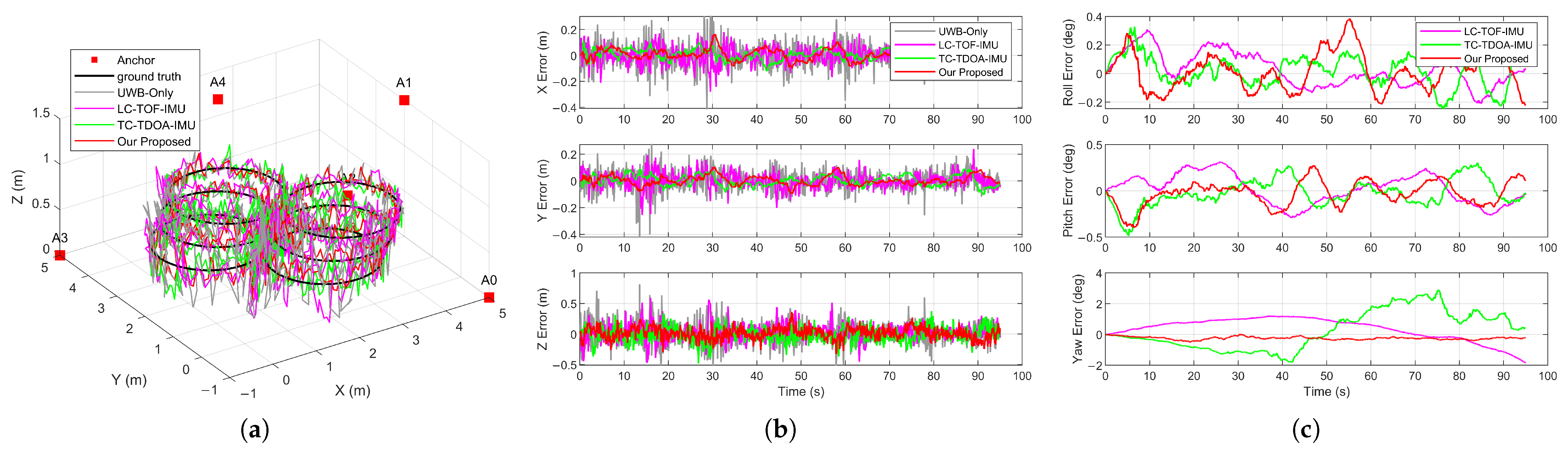
Figure 6a shows the true path of trajectory 1 and each algorithm’s 3D position estimation results. It was observed that the UWB-only algorithm exhibited the largest trajectory error magnitude. In contrast, the trajectory estimated by the proposed algorithm maintained good consistency with the ground truth during turns and altitude changes. Figure 6b compares the position errors of each algorithm along the X, Y, and Z axes. The UWB-only algorithm showed the largest magnitude of error. Due to the lack of a motion model for the UAV, the UWB-only algorithm is susceptible to TDOA measurement noise and rapid changes in UAV dynamics, leading to degraded positioning accuracy. In contrast, various UWB/IMU fusion algorithms exhibited errors within ±0.3 m in the X and Y axes and within ±0.6 m in the Z axis, demonstrating higher accuracy and stability. The position error fluctuations of LC-TOF-IMU were higher than those of TC-TDOA-IMU and the proposed algorithm. This is primarily because the loosely coupled method uses the positioning results of the UWB system as measurements for state updates. In contrast, the tightly coupled methods directly utilize the raw measurements of the UWB system. When a UWB measurement has a large error causing degraded positioning accuracy, LC-TOF-IMU propagates this error directly into the state update process, causing fluctuations in state variable estimation. TC-TDOA-IMU and the proposed algorithm effectively disperse the impact of a single measurement error by introducing multiple independent TDOA measurements, thereby improving positioning accuracy and stability.

Figure 6c compares the attitude errors of various UWB/IMU fusion algorithms for trajectory 1. The UWB-only algorithm cannot provide attitude information and is therefore excluded from the comparison. The three fusion algorithms exhibited similar errors in the roll and pitch directions, with error fluctuations maintained within ±0.5°. Even under dynamic scenarios such as climbs and turns, the estimation accuracy for roll and pitch angles remained stable, demonstrating the good performance of the proposed algorithm in attitude estimation. There were significant differences in the accuracy of yaw angle estimation among the different fusion algorithms. The maximum errors in the yaw direction for LC-TOF-IMU, TC-TDOA-IMU, and the proposed algorithm were 1.85°, 2.92°, and 0.49°, respectively. LC-TOF-IMU and TC-TDOA-IMU update the state using the UWB positioning results and TDOA measurements, respectively. Due to the absence of direct measurements of the yaw angle and the weak observability of the yaw angle from position-only measurements, these algorithms suffer from accumulated errors caused by IMU bias and noise, resulting in noticeable yaw drift. In contrast, the proposed algorithm fuses AOA measurements, providing direct observational constraints for the yaw angle during the state update process, effectively enhancing the stability and accuracy of yaw angle estimation.

The RMSEs for position and attitude estimation of each algorithm in trajectory 1 are shown in

Table 5. RMSEs of position and attitude estimates for different localization algorithms in the simulation.

Trajectory	Algorithm	Positioning Error (m)				Attitude Error (Deg)
		X	Y	Z	3D	ϕ	θ	ψ
1	UWB-only	0.086	0.071	0.175	0.208	—	—	—
	LC-TOF-IMU	0.057	0.053	0.128	0.150	0.12	0.16	0.81
	TC-TDOA-IMU	0.039	0.039	0.113	0.126	0.11	0.15	1.28
	Proposed	0.043	0.035	0.093	0.108	0.13	0.14	0.26
2	UWB-only	0.095	0.106	0.198	0.244	—	—	—
	LC-TOF-IMU	0.068	0.090	0.142	0.181	0.34	0.38	1.94
	TC-TDOA-IMU	0.040	0.039	0.097	0.112	0.11	0.08	0.97
	Proposed	0.033	0.042	0.097	0.111	0.12	0.06	0.41
3	UWB-only	0.081	0.069	0.164	0.196	—	—	—
	LC-TOF-IMU	0.062	0.047	0.112	0.136	0.17	0.39	1.86
	TC-TDOA-IMU	0.048	0.036	0.106	0.122	0.12	0.17	1.88
	Proposed	0.028	0.025	0.081	0.089	0.10	0.08	0.19

. Consistent with the static initialization results, all algorithms exhibited larger position errors in the Z axis direction than on the X and Y axes. Algorithms incorporating IMU significantly reduced position errors in all three directions. Among the fusion algorithms, LC-TOF-IMU yielded the lowest positioning accuracy, with RMSEs along the X, Y, and Z axes being 66%, 75%, and 73% of those of the UWB-only algorithm, respectively. Benefiting from the direct fusion of TDOA measurements with IMU data, TC-TDOA-IMU and the proposed algorithm exhibited optimal positioning performance, with 3D RMSEs of 0.126 m and 0.108 m, respectively. AOA has lower observation sensitivity to the position and is primarily used for updating and correcting the UAV’s heading. The improvement in position accuracy offered by the proposed algorithm over the conventional UWB/IMU tightly coupled method is relatively small. However, compared to the conventional UWB/IMU loosely coupled method, it improved position accuracy by approximately 25%, 34%, and 27% in the X, Y, and Z axes, respectively. For attitude estimation in trajectory 1, all three fusion algorithms achieved similar accuracy in roll and pitch angles, with RMSEs below 0.2°. By incorporating AOA measurements, the proposed algorithm effectively improved yaw angle estimation, reducing the yaw angle RMSE to 0.26°, which is significantly lower than that of LC-TOF-IMU (0.81°) and TC-TDOA-IMU (1.28°). These results demonstrate that conventional algorithms relying solely on position measurements are insufficient for accurate yaw angle estimation, whereas the proposed algorithm achieved higher accuracy and stability in overall attitude estimation.

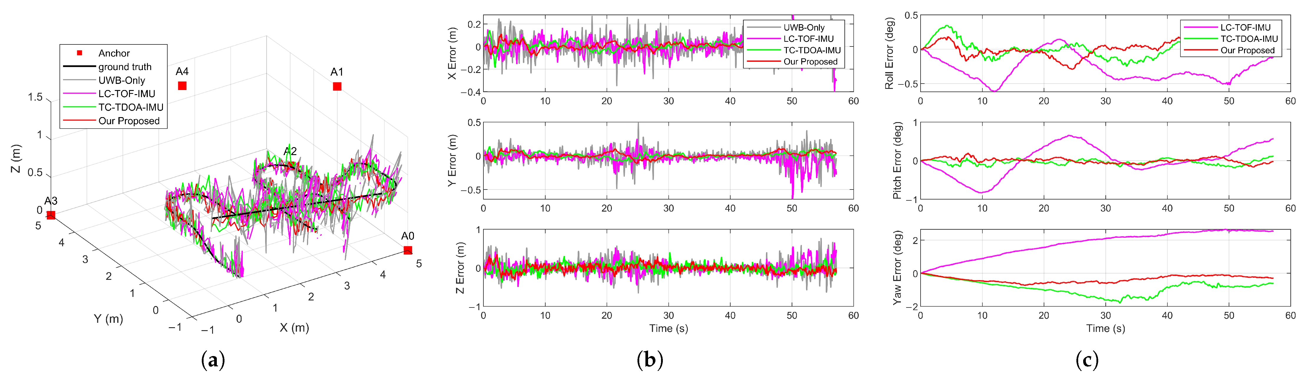
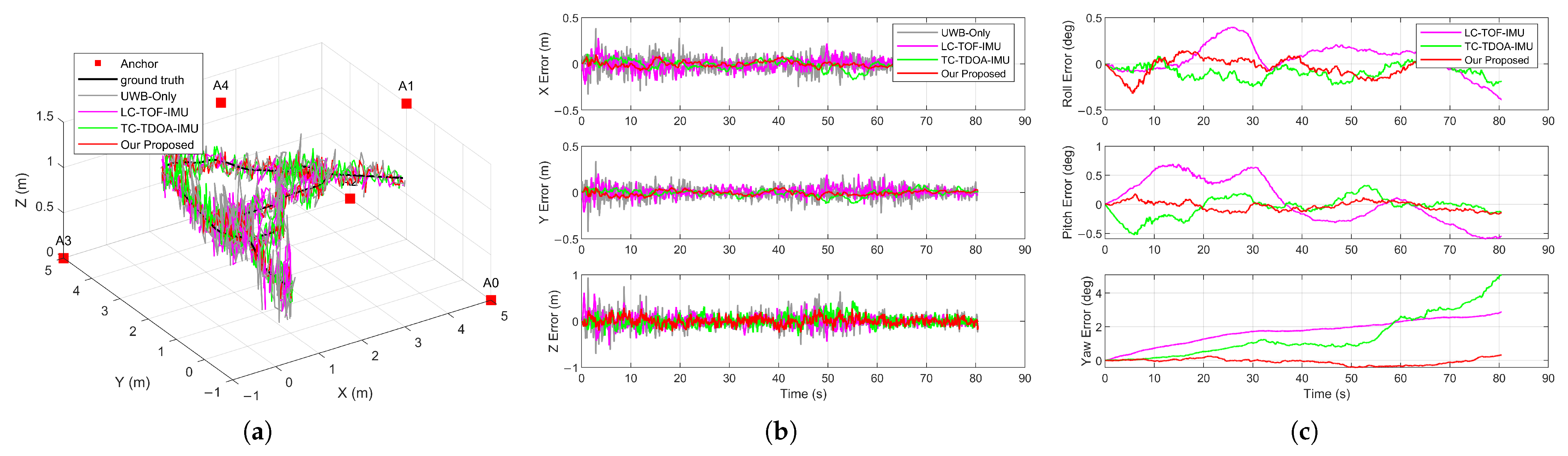
In trajectories 2 and 3, the UAV executed more complex flight maneuvers, increasing the frequency of attitude changes and the amplitude of altitude fluctuations. Figure 7 and Figure 8 show each algorithm’s localization and attitude estimation results for these two trajectories. In terms of position estimation, the proposed algorithm achieved 3D RMSEs of 0.111 m and 0.089 m for the two trajectories, demonstrating the best accuracy and validating the robustness of the constructed tightly coupled framework in dynamic scenarios. Consistent with trajectory 1, conventional algorithms exhibited large errors in the yaw direction, with RMSEs close to 2°. The proposed algorithm, which introduces AOA measurements to correct the UAV heading, controlled the yaw angle error to 0.41° and 0.19° in trajectories 2 and 3, significantly outperforming LC-TOF-IMU (1.94°, 1.86°) and TC-TDOA-IMU (0.97°, 1.88°) and showing a clear advantage in attitude estimation accuracy and stability.

Figure 9 compares yaw angle estimation results under different initial yaw bias conditions. TC-TDOA-IMU was configured with initial yaw angle errors of 15°, 30°, and 60°, while the initial bias for the proposed algorithm was set to 60°. As the UAV moved, the yaw angle estimates for all three TC-TDOA-IMU configurations gradually converged to the correct value. However, the convergence rate depends significantly on the magnitude of the initial yaw angle error. With a 15° bias, the system required approximately 10 s to achieve stable convergence, while with a 60° initial error, TC-TDOA-IMU required nearly 38 s to first reduce the yaw angle error below 3°. Although the proposed algorithm started with an initial yaw angle error of 60° without using the initialization algorithm specifically for this test, it was able to achieve rapid state correction early in the flight through AOA measurements. The yaw angle estimate converged quickly to the ground truth within seconds and maintained high consistency with the true value during subsequent motion. The results indicate that the proposed algorithm has a strong tolerance to initial state errors, significantly outperforming conventional algorithms, which exhibit long-term drift and slow convergence under conditions with large bias.

4.2. Experiment

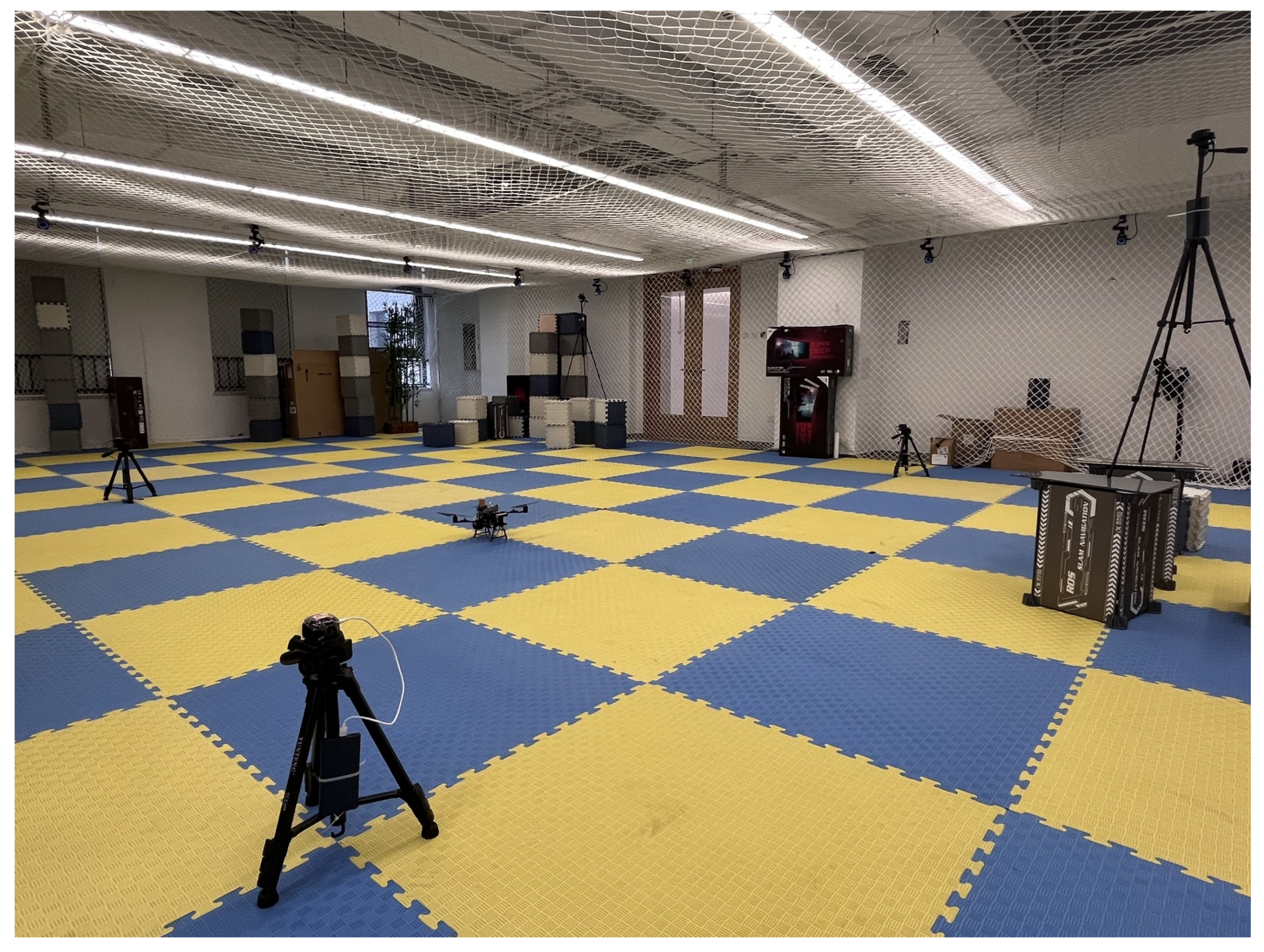
To verify the effectiveness of the proposed indoor navigation system based on UWB/IMU, flight experiments were conducted in an indoor area equipped with an OptiTrack motion capture system (Virtual Point, Beijing, China). The experimental area, as shown in Figure 10, measured approximately 10 m × 10 m × 3 m. The motion capture system consisted of 18 Prime X 13W infrared cameras (OptiTrack, Corvallis, OR, USA) mounted on the ceiling of the experimental area. It provided high-precision position and attitude measurements at a frequency of 100 Hz, with a positional error of less than ±0.30 mm and a rotational error of less than 0.5 degrees. The system output served as the ground truth reference for UAV state estimation. Five UWB anchors were deployed in the experimental area. Their positions were precisely calibrated using the motion capture system, with coordinates given as follows: $A_0(-1.99,0.51,-3.01)$, $A_1(3.02,0.48,-2.04)$, $A_2(-0.95,0.49,3.02)$, $A_3(-3.09,1.89,0.02)$, $A_4(3.09,1.91,3.01)$. The onboard UWB tag outputted TDOA and AOA measurements at a frequency of 10 Hz, while the IMU provided three-axis angular velocity and acceleration data at 200 Hz.

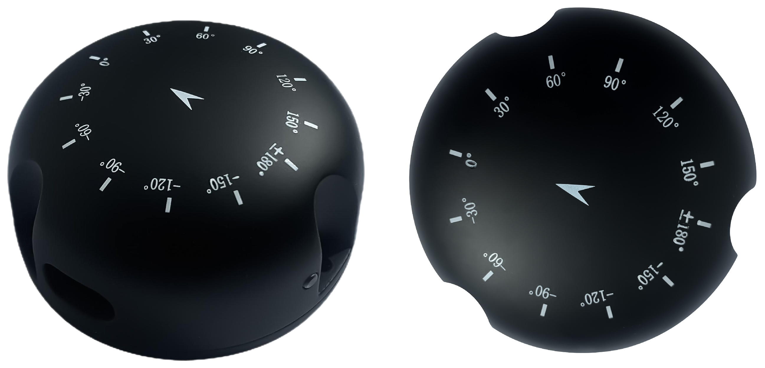
Due to the significant nonlinear characteristics of AOA measurement errors in different directions, the raw AOA measurements from the UWB tag required calibration. The UWB tag to be calibrated was fixed on a high-precision electric turntable and rotated continuously through 360° in 1° steps. One hundred sets of AOA measurement data were collected at each angle and averaged to establish the mapping relationship between ground truth and observed values. Figure 11 illustrates the nonlinear correspondence between ground truth and average measured values during the AOA calibration process.

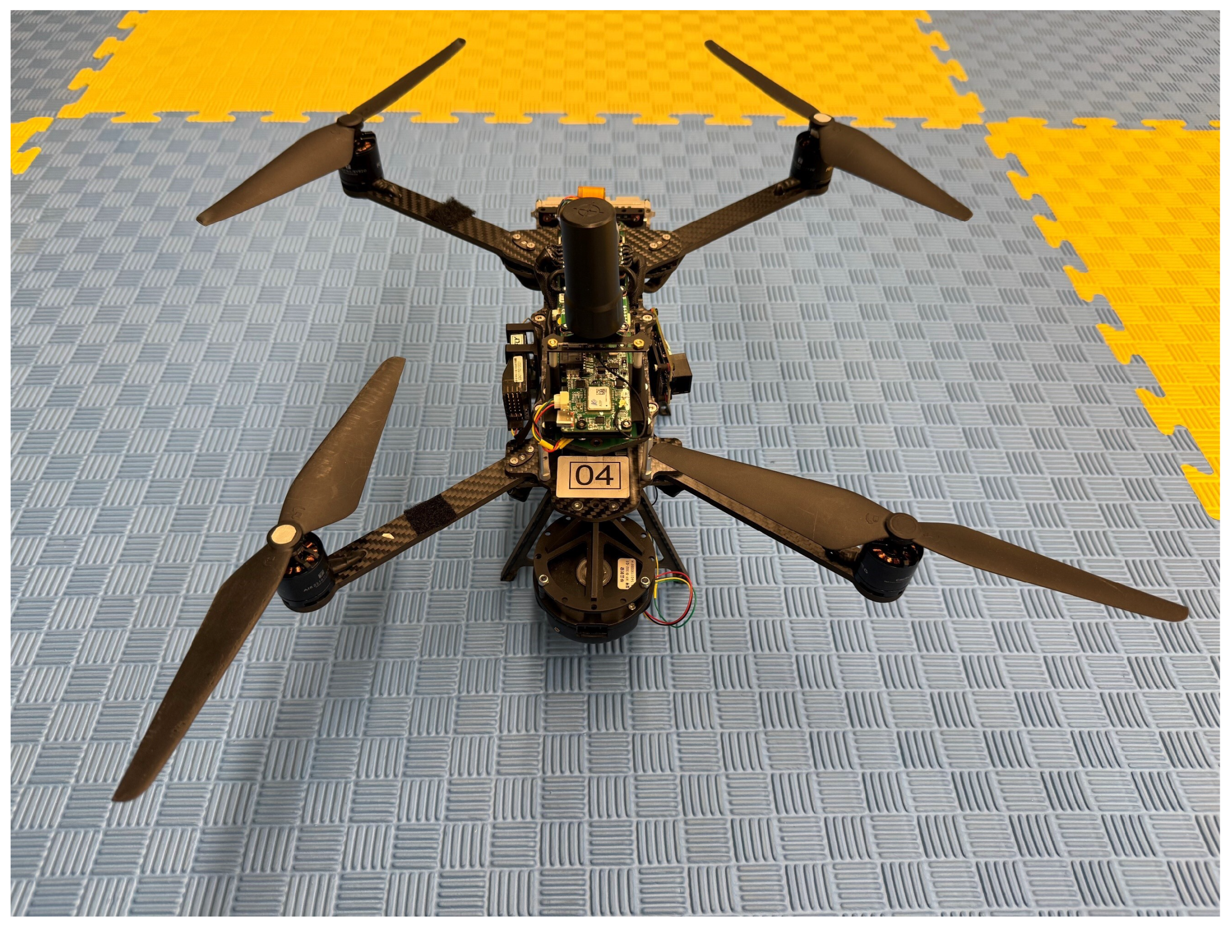
To evaluate the performance of the proposed algorithm, flight experiments were conducted by simultaneously controlling two UAVs (UAV 01 and UAV 02) in the indoor environment. Both UAVs remained static on the ground for 1 s to complete the initialization process then completed their flights and landings in approximately 80 s and 105 s, respectively. To cover various flight attitude changes, UAV 01 took off with a non-horizontal attitude and exhibited larger maneuvering amplitudes during flight, with maximum absolute roll and pitch angles reaching 33° and 36°. UAV 02 took off horizontally, with smoother attitude changes, maintaining roll and pitch angles within ±10°. Similar to the simulation, three comparison algorithms were set up: UWB-only, LC-TOF-IMU, and TC-TDOA-IMU. To ensure fairness, all algorithms used the same initial values provided by the initialization algorithm.

Table 6. Ground truth and estimated position and attitude of UAVs during initialization.

UAV	Ground Truth Position (m)	Ground Truth Attitude (RPY) (Deg)	Estimated Position (m)	Estimated Attitude (RPY) (Deg)
UAV 01	1.06, −0.32, 0.14	0.1, 15.3, −149.3	1.02, −0.30, 0.18	0.2, 14.9, −150.6
UAV 02	2.74, 1.22, 0.12	−0.4, 0.6, 158.2	2.80, 1.25, 0.07	−0.6, 1.4, 158.7

summarizes the position and attitude estimation results for UAV 01 and UAV 02 during the initialization phase, compared with the ground truth provided by the motion capture system. The position estimation errors for the two UAVs were 0.06 m and 0.08 m, respectively, meeting the initial state accuracy requirements of the integrated navigation system. UAV 01 maintained a non-horizontal attitude while static, with a pitch angle of 15.3°, while UAV 02 was approximately level. In terms of attitude estimation, the errors for the three attitude angles (roll, pitch, yaw) of both UAVs were controlled within 1°, verifying that the proposed initialization algorithm can provide reliable estimates under different attitude conditions. The initialization accuracy was primarily limited by UWB measurement noise. Accumulating more measurements could reduce position and yaw angle estimation errors but correspondingly increase initialization latency.

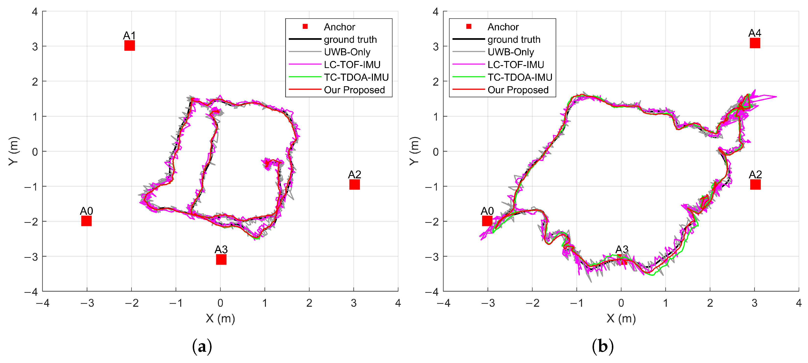
Figure 12a shows the horizontal trajectory of UAV 01 under different localization algorithms. Benefiting from the centimeter-level ranging accuracy of the UWB system, all algorithms were able to track the basic motion of the UAV. UWB-only and LC-TOF-IMU exhibited larger positioning jitter and errors, indicating that these two algorithms are more sensitive to ranging noise and cannot suppress positioning errors. The horizontal positioning results for UAV 02 are shown in Figure 12b. Its flight range was wider, and the trajectory passed through edge areas of the system (e.g., near A0 and A3) multiple times. Due to degraded observation geometry in such areas, the positioning accuracy of UWB-only and LC-TOF-IMU significantly decreased. In contrast, the proposed algorithm fuses multi-source measurements (TDOA and AOA) and corrects the UAV state based on measurement residuals, maintaining a stable trajectory even in regions with weak observability and demonstrating stronger robustness. However, despite the richer observation information, the proposed algorithm may still experience reduced positioning accuracy at the edges of the system. In practical deployment, anchors should be placed at sufficient distances apart, covering a sufficiently large area, while the UAV should ideally operate in non-edge regions to achieve optimal system performance.

Table 7. RMSEs of position and attitude estimates for different localization algorithms in flight experiments.

UAV	Algorithm	Positioning Error (m)				Attitude Error (Deg)
		X	Y	Z	3D	ϕ	θ	ψ
01	UWB-only	0.057	0.057	0.194	0.210	—	—	—
	LC-TOF-IMU	0.056	0.051	0.165	0.181	1.45	1.77	1.17
	TC-TDOA-IMU	0.039	0.040	0.128	0.140	1.36	1.50	1.22
	Proposed	0.038	0.037	0.121	0.132	1.32	1.54	0.48
02	UWB-only	0.064	0.082	0.207	0.231	—	—	—
	LC-TOF-IMU	0.072	0.077	0.180	0.209	0.65	0.44	2.34
	TC-TDOA-IMU	0.043	0.088	0.142	0.172	0.69	0.66	2.28
	Proposed	0.037	0.077	0.137	0.161	0.67	0.67	0.28

provides the positioning errors of each algorithm along the three axes. The proposed algorithm achieves the best positioning accuracy among all compared algorithms, with errors of (0.038, 0.037, 0.121) m and (0.037, 0.077, 0.137) m along the X, Y, and Z axes for UAV 01 and UAV 02, respectively. The Z axis positioning error is significantly higher than in the planar directions. Due to height constraints in the indoor space, it is challenging to improve vertical positioning accuracy by increasing the vertical separation of anchors. The proposed algorithm could be further fused with sensors like barometers to enhance Z axis positioning accuracy. Figure 13 statistically analyzes the positioning errors for all flight data, validating the advantage of the proposed algorithm in positioning accuracy. Compared to UWB-only and the conventional LC-TOF-IMU, the proposed algorithm reduced the average 3D RMSE by 33.7% and 25.0%, respectively, effectively mitigating the impact of ranging errors on positioning accuracy. The performance improvement primarily benefits from the introduction of IMU dynamic information and enhancements in the data fusion algorithm.

Table 7 also summarizes the RMSEs for attitude estimation of each algorithm. Compared to simulation results, the roll and pitch errors for UAV 01 and UAV 02 increased, which may be attributed to real-world factors such as airframe vibration and aerodynamic disturbances during actual flight, which increased gyroscope measurement noise and affected attitude estimation accuracy. UAV 01 experienced larger attitude changes during flight, with roll and pitch RMSEs of approximately 1.3° and 1.6°. These are higher than those of UAV 02, indicating that highly dynamic flight may adversely affect attitude estimation accuracy. The estimation of roll and pitch angles primarily relies on IMU propagation, with UWB measurements providing only indirect corrections. Hence, the estimation accuracy differences among algorithms in these directions are minor. This result is consistent with the simulation analysis. On the other hand, yaw angle estimation primarily depends on angular velocity measurements from the IMU. Due to the cumulative effects of gyroscope measurement noise and the limited ability to observe yaw angle from range-based measurements, traditional methods encounter difficulties in achieving high-precision yaw angle estimation. As seen in Table 7, there are significant differences in yaw angle estimation accuracy among the different algorithms. Taking UAV 02 as an example, the yaw angle RMSEs for LC-TOF-IMU and TC-TDOA-IMU reached 2.34° and 2.28°, respectively. The proposed algorithm, by introducing AOA measurements to participate in yaw angle correction directly, significantly reduced the yaw angle estimation error during the flights of both UAV 01 and UAV 02, achieving RMSEs of 0.48° and 0.28°, representing an average reduction of 73.5%. These results demonstrate that the proposed algorithm exhibits good accuracy and robustness in localization and attitude estimation under complex flight conditions, showing significantly higher accuracy and faster convergence in yaw angle estimation than conventional algorithms.

5. Conclusions

Navigation of UAVs in indoor environments still faces numerous challenges. Although UWB-based positioning systems offer decimeter-level accuracy, their robustness is limited and cannot provide attitude information. Conventional UWB/IMU fusion algorithms perform poorly in attitude estimation, particularly in yaw angle estimation, while the TWR scheme limits the capacity and scalability of the positioning system. This paper develops a TC–ESKF-based UWB/IMU integrated navigation system to address these limitations. First, AOA measurements are obtained using an onboard UWB antenna array, compensating for the lack of attitude perception in traditional UWB systems. Subsequently, an initialization algorithm suitable for static conditions is proposed, which fuses UWB measurements with accelerometer data to rapidly estimate the initial position and attitude without relying on a magnetometer. The initialization results provide a reliable initial condition for the subsequent state estimation process. On this basis, a tightly coupled UWB/IMU fusion framework is developed, in which TDOA, AOA, and IMU measurements are integrated using the ESKF, enabling 6-DoF state estimation for the UAV. The real-world flight experiments validate the effectiveness of the proposed system. Compared with representative fusion algorithms, it achieves a 25.0% reduction in 3D positioning RMSE and a 73.5% reduction in yaw angle RMSE, demonstrating superior performance in both localization accuracy and robustness. Future work will focus on analyzing the impact of UWB measurement errors under NLOS conditions. This analysis will investigate how such errors affect both position and attitude estimation and will explore the development of fusion strategies to mitigate these effects. Additionally, the performance of the system in scenarios with limited anchor placement and anchor numbers will be analyzed and optimized. These aspects are critical for further enhancing the system’s performance in complex indoor environments.