
Autonomous Trajectory Control for Quadrotor eVTOL in Hover and Low-Speed Flight via the Integration of Model Predictive and Following Control


Abstract
1. Introduction
- (1)
- A high-fidelity simulation model, incorporating rotor flapping dynamics, differential collective pitch control, and enhanced aerodynamic interference effects, is developed to realistically capture nonlinear flight behavior.
- (2)
- A novel hierarchical control architecture is proposed, combining the predictive and constraint-handling advantages of MPC with the fast command execution of EMFC. This design balances computational demands with accurate trajectory-tracking performance.
- (3)
- The effectiveness of the proposed framework is validated through four representative ADS-33E-PRF mission tasks, showing strong compliance with ADS-33E-PRF-desired criteria in low-speed flight conditions.
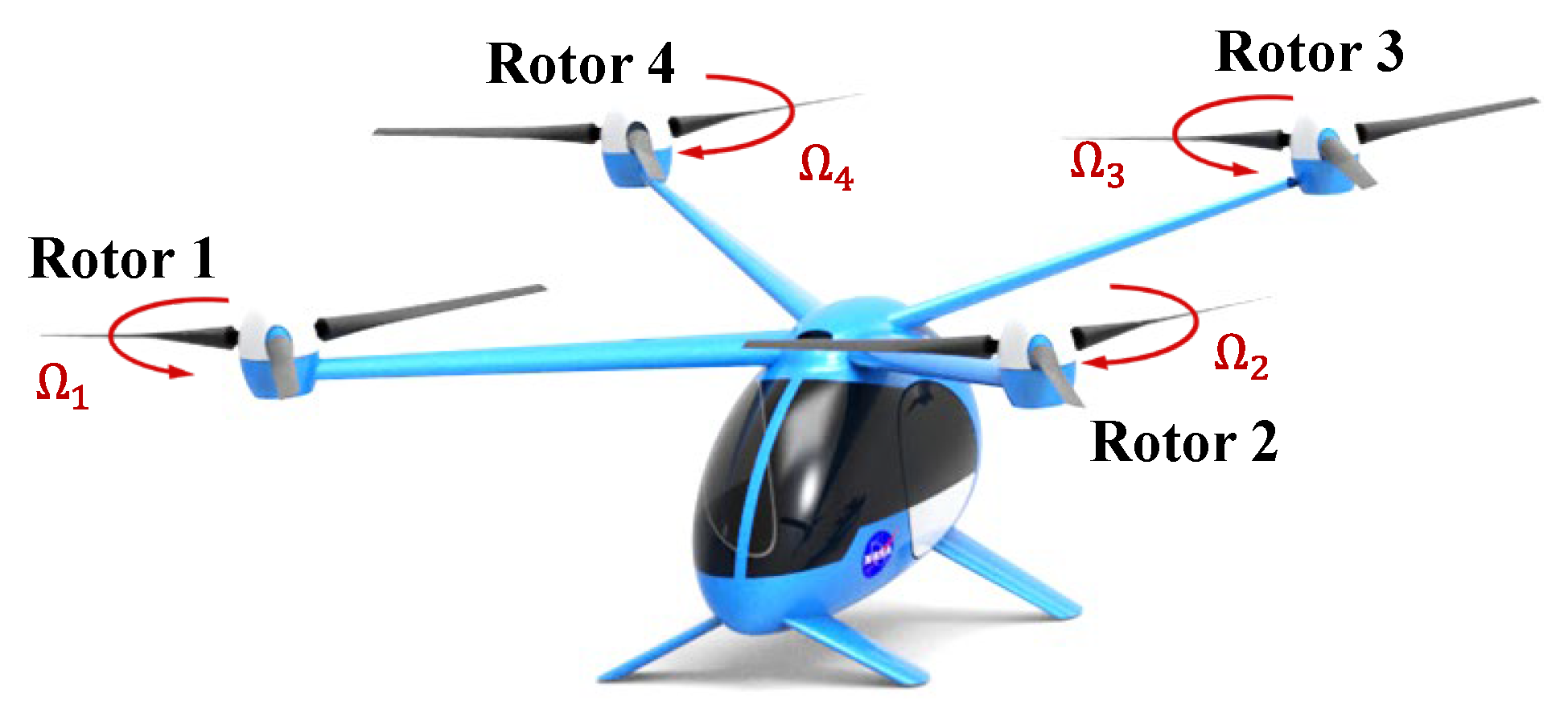
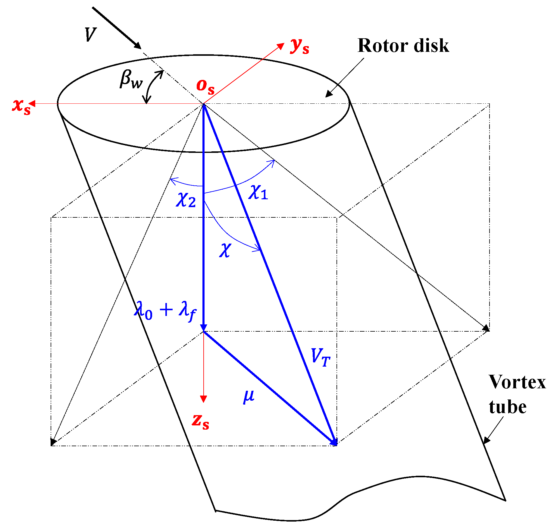
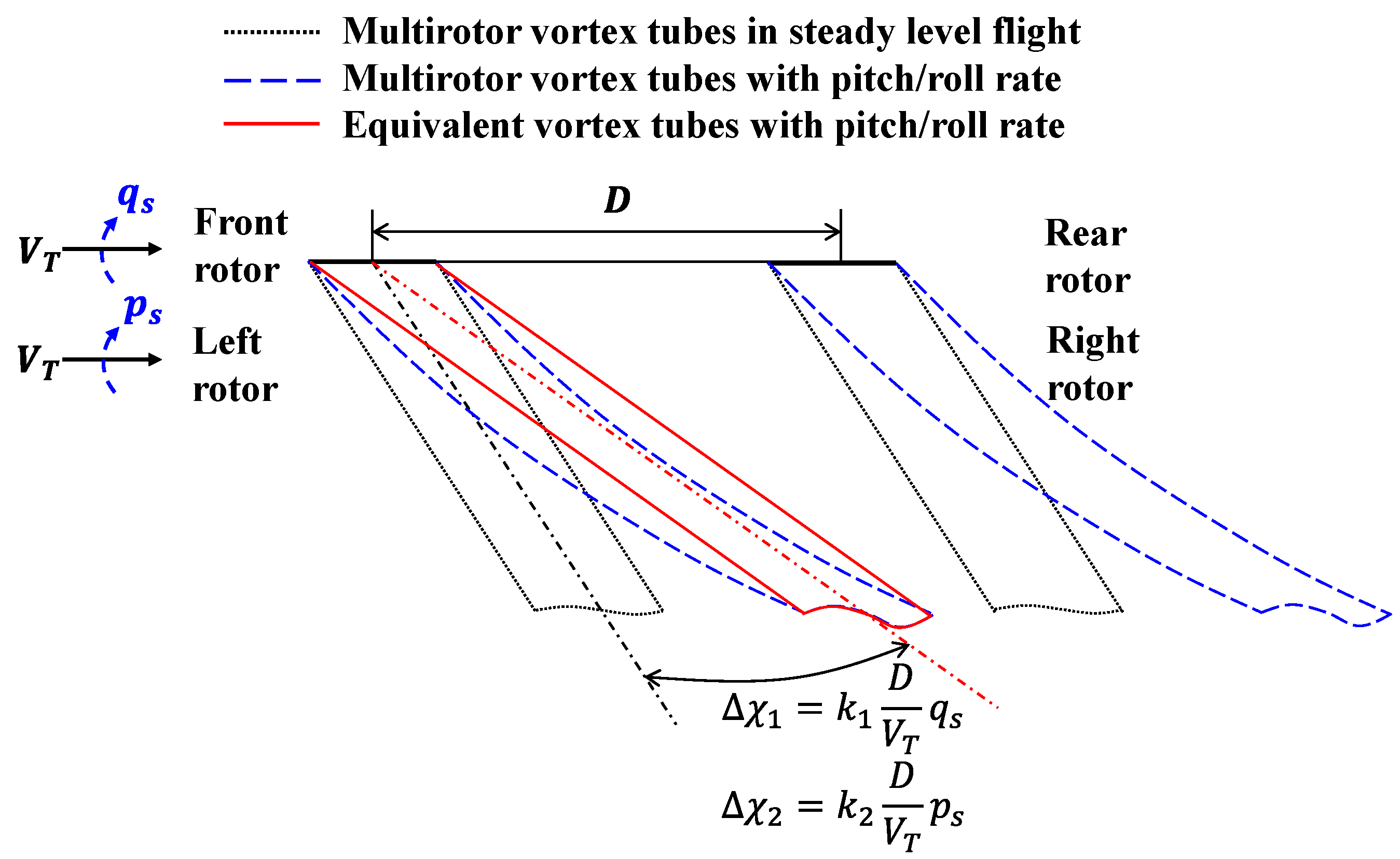
2. Flight Dynamic Modeling with Multirotor Aerodynamic Interference
- represents the rigid-body states of the quadrotor platform,
- for denote the rotor-specific dynamic states for the four rotors, defined as
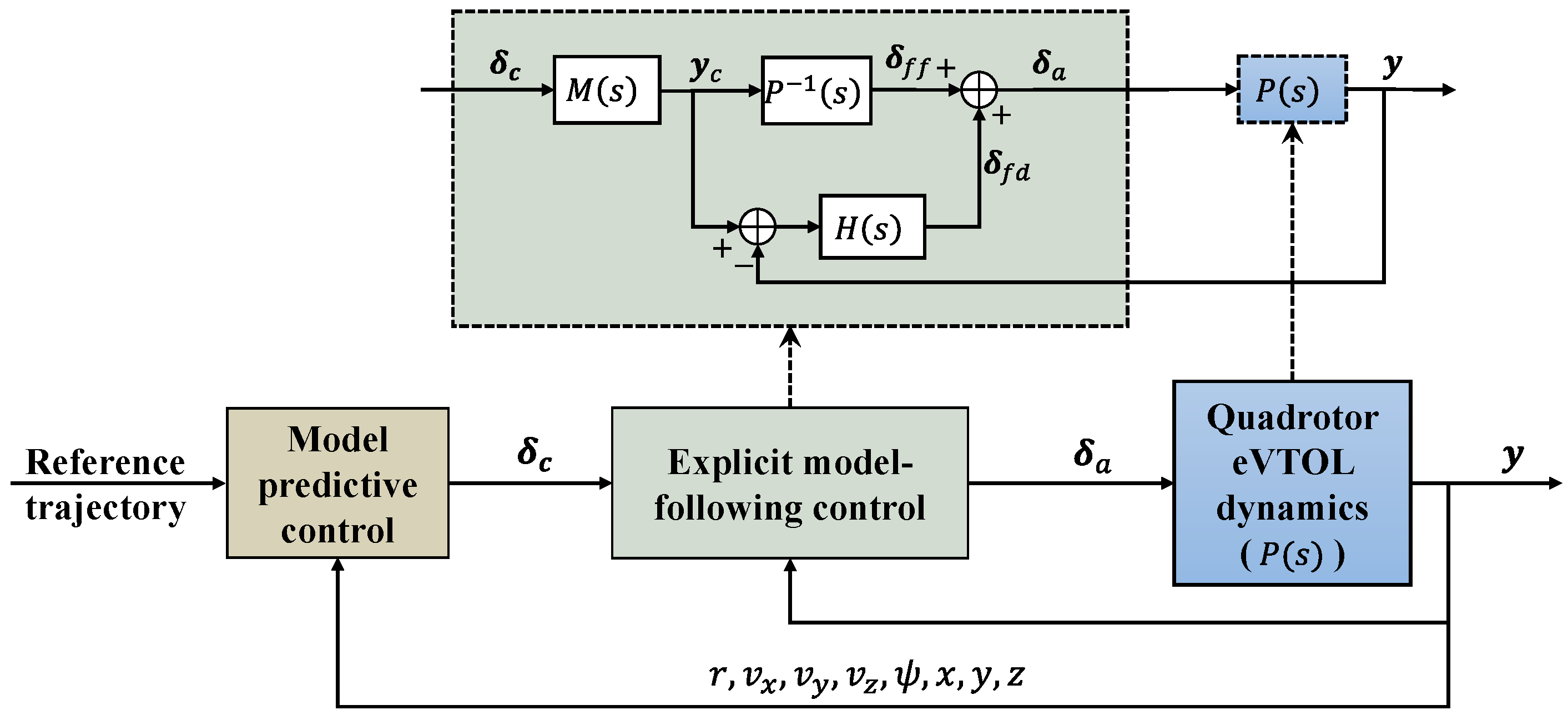
3. Hierarchical Control Architecture
3.1. Explicit Model-Following Control Design
3.2. Model Predictive Control Formulation
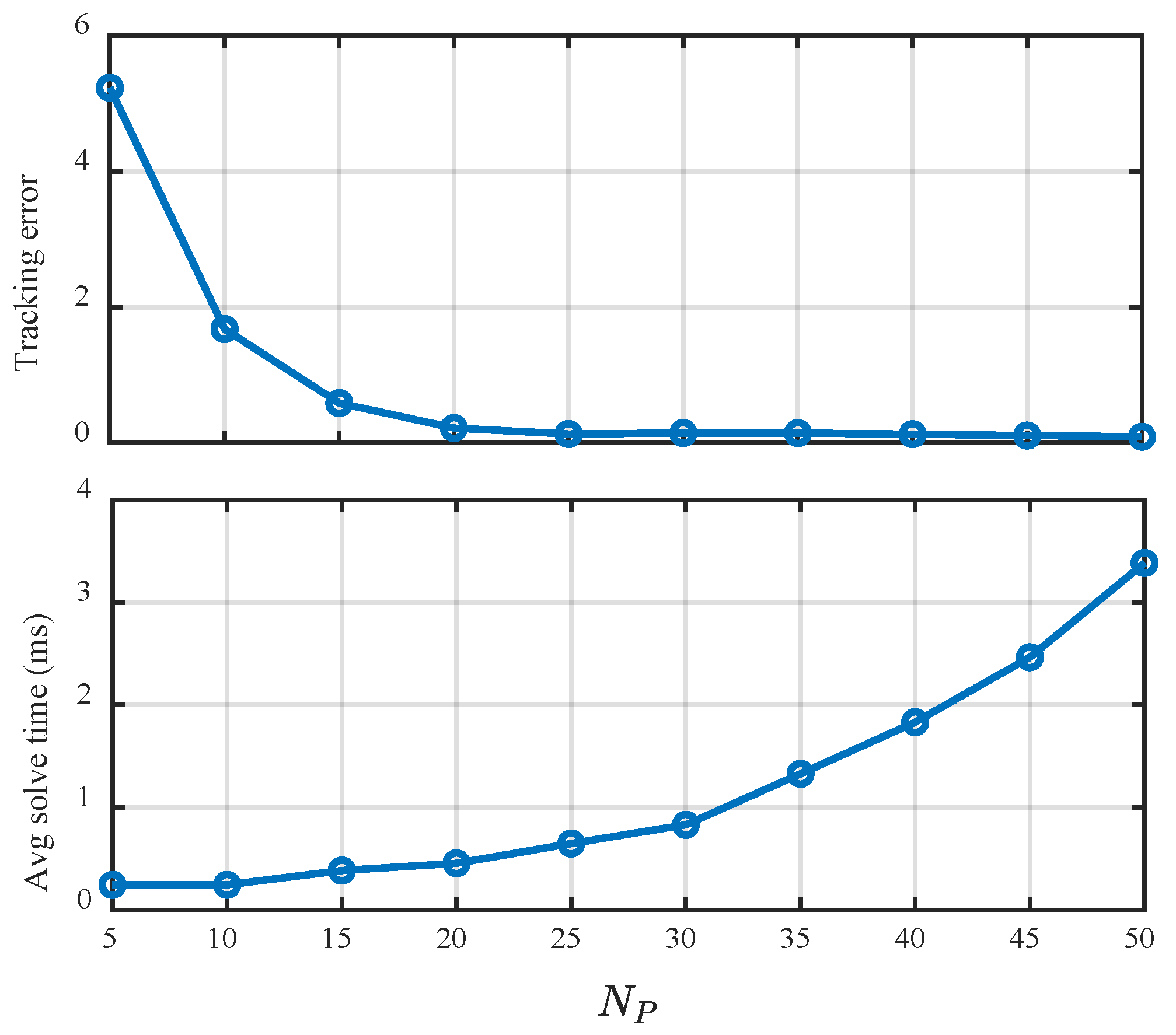
3.3. Parameter Tuning and Stability Analysis
4. Numerical Simulations and Performance Evaluation
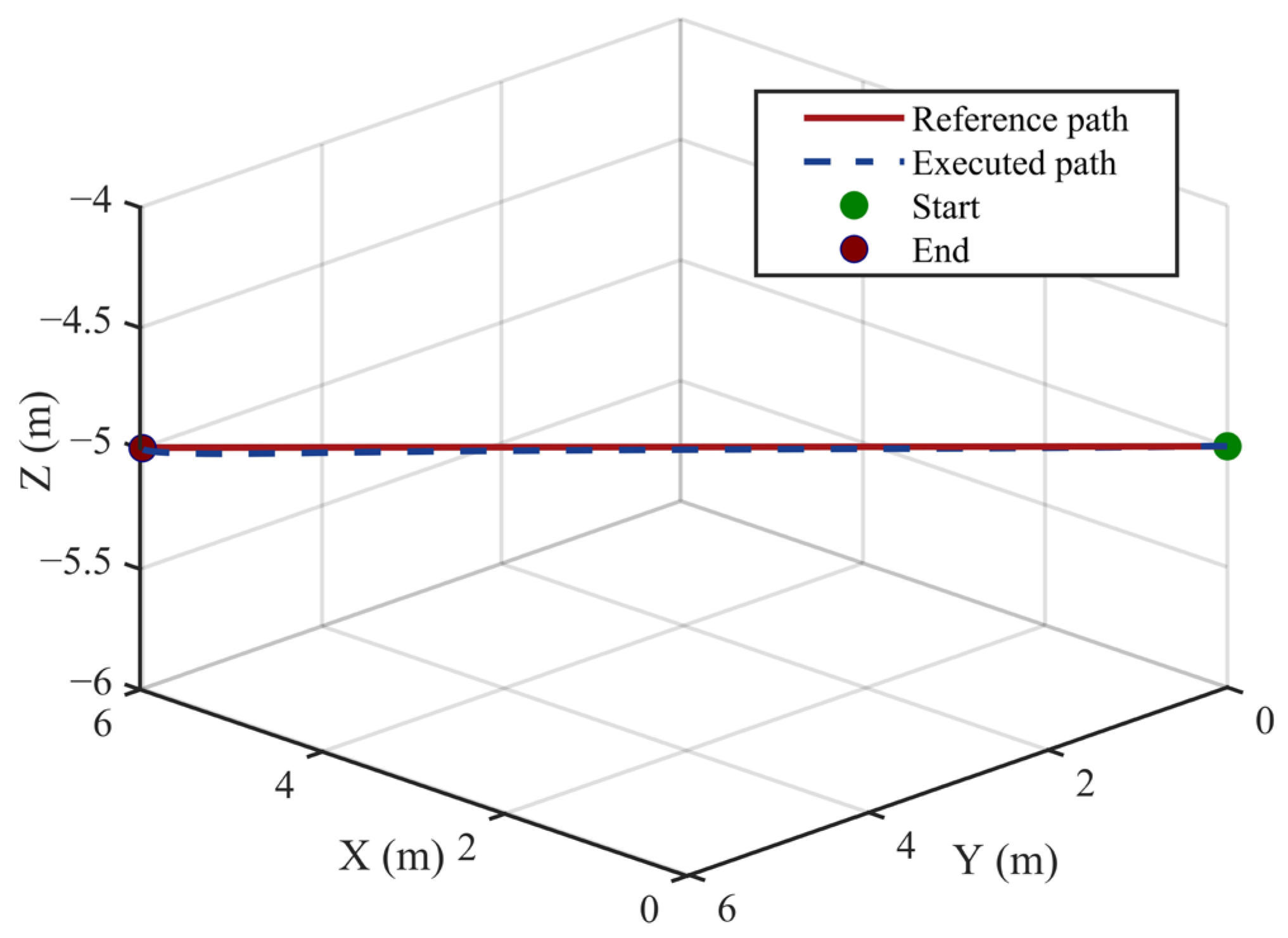
4.1. Hover
4.2. Hovering Turn
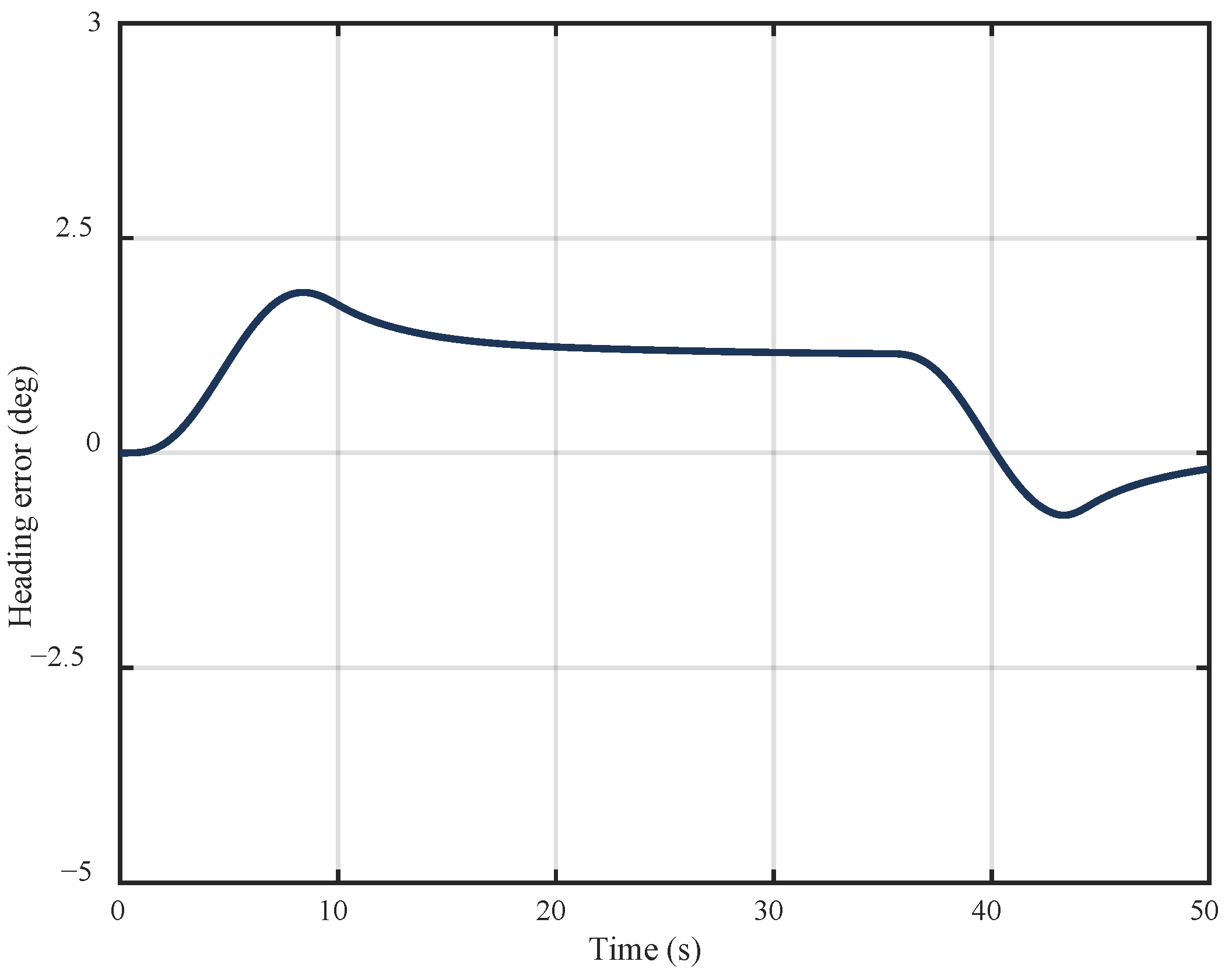
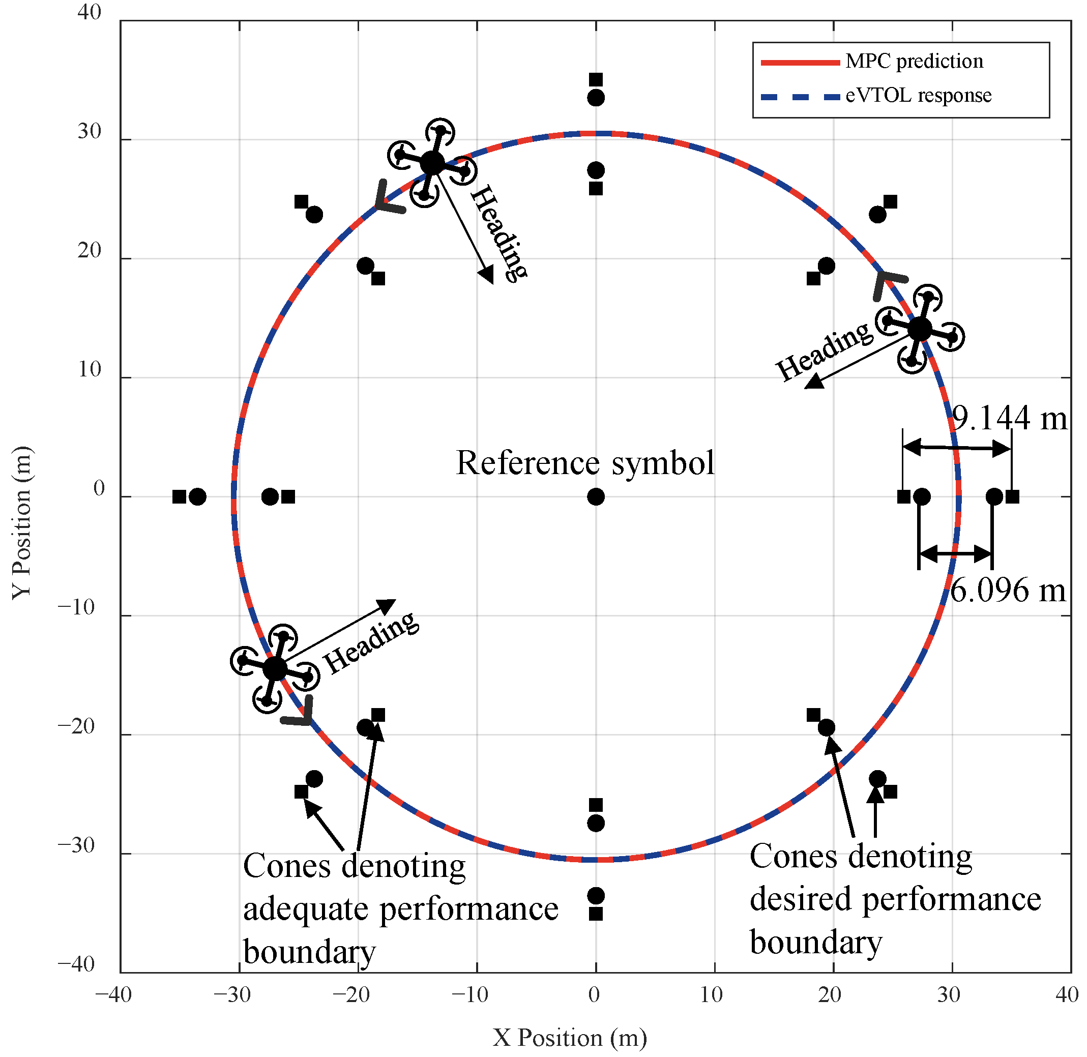
4.3. Pirouette
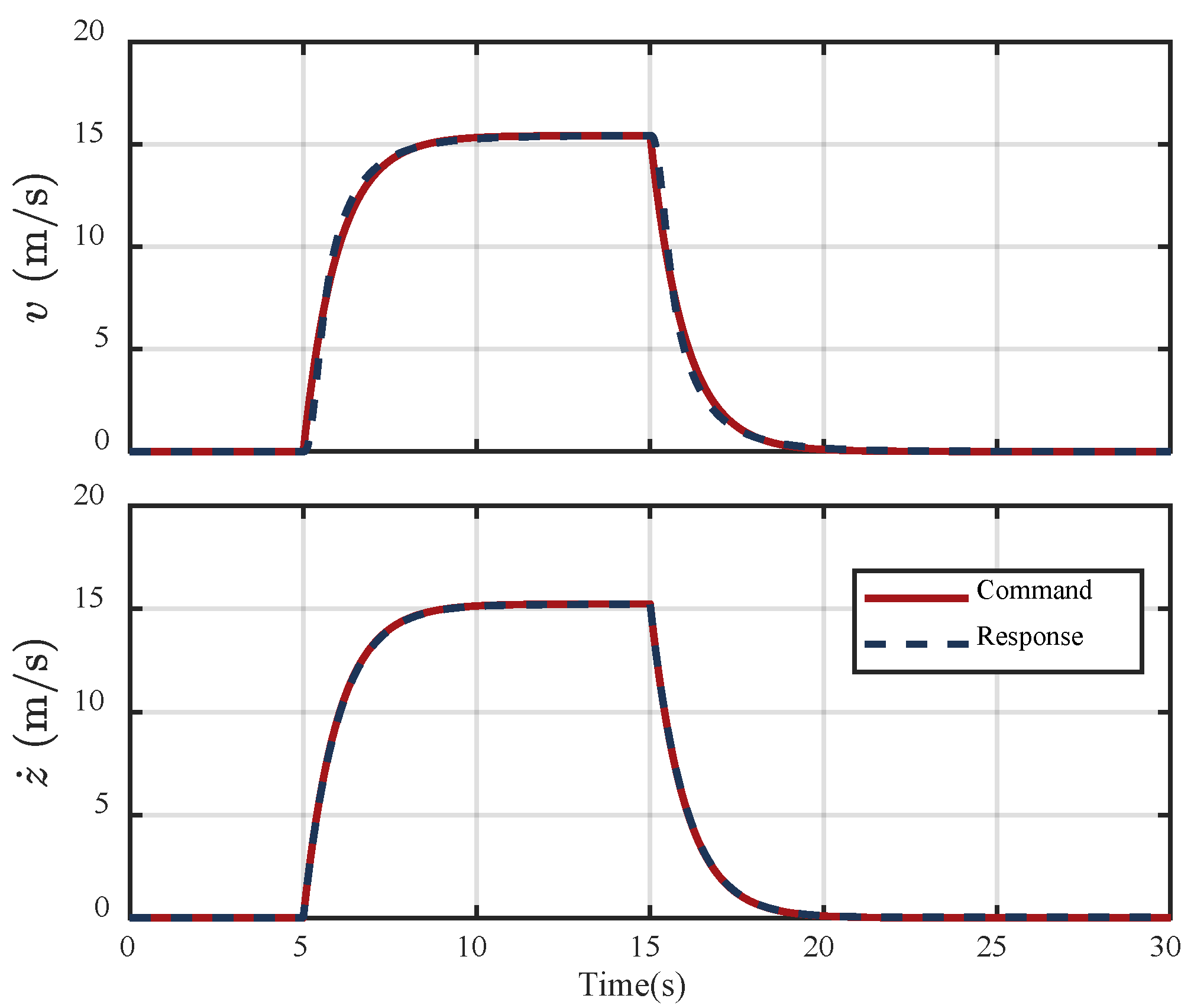
4.4. Vertical Maneuver
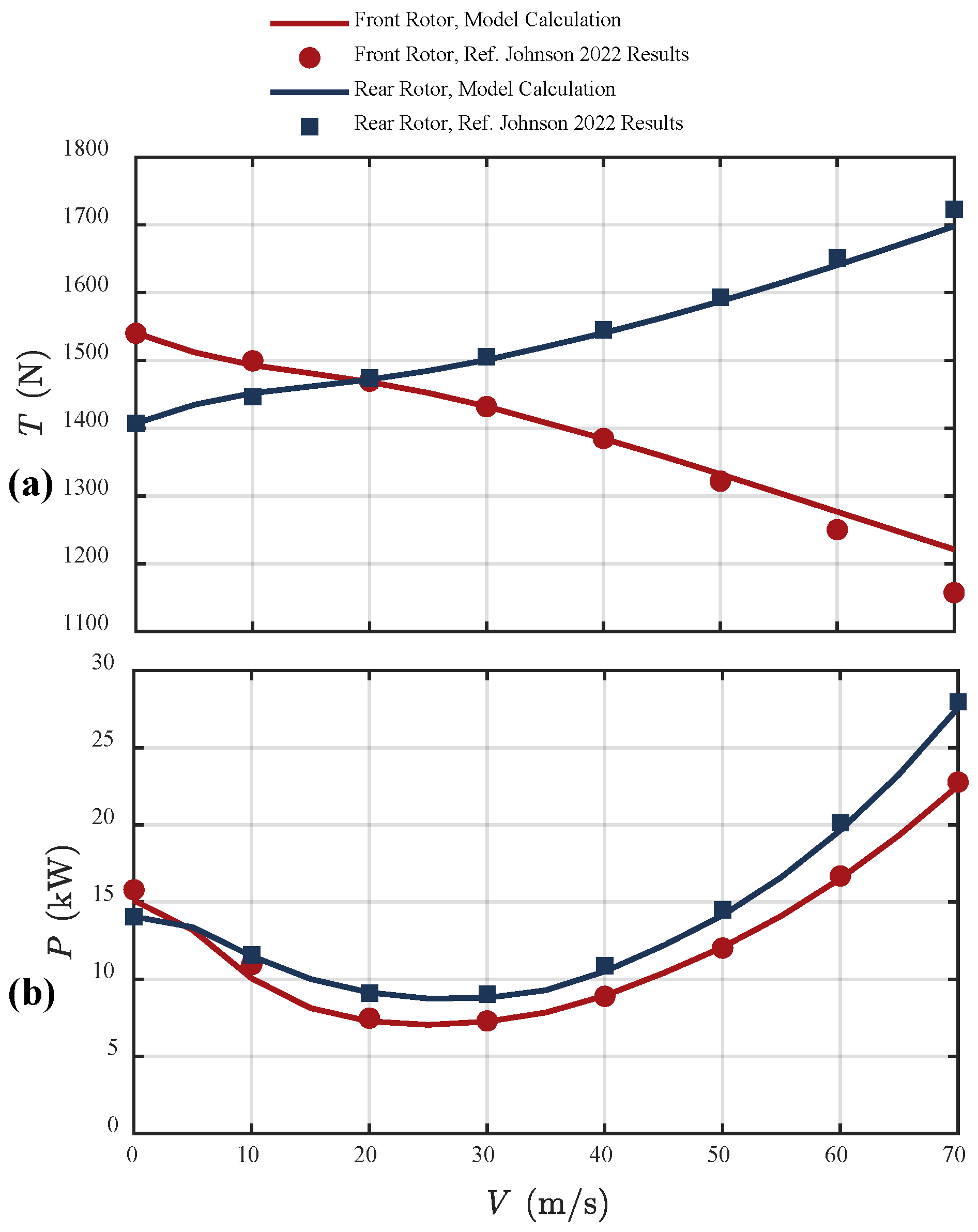
5. Discussion
6. Conclusions
- Aerodynamic interference between rotors was explicitly modeled, and the developed flight dynamics model successfully captured these effects to replicate real conditions;
- By separating the planning task from the fast-response control task, the architecture achieved a clear division of roles, maintaining system stability while improving computational efficiency;
- Flight simulations on four representative ADS-33E-PRF tasks demonstrated accurate and stable trajectory tracking, with all desired performance criteria fully satisfied.
7. Limitations and Future Work
Author Contributions
Funding
Data Availability Statement
Conflicts of Interest
Appendix A
- During the acceleration phase (), the tangential velocity is
- In the constant-speed cruise phase (), the tangential velocity is held constant,
- During the deceleration phase (), the same quintic profile is used in reverse to smoothly reduce velocity to zero,
References
- Doff-Sotta, M.; Cannon, M.; Bacic, M. Data-driven robust model predictive control of tiltwing vertical takeoff and landing aircraft. J. Guid. Control Dyn. 2025, 48, 203–211. [Google Scholar] [CrossRef]
- Wang, S.; Lima Pereira, L.T.; Ragni, D. Design exploration of UAM vehicles. Aerosp. Sci. Technol. 2025, 160, 110058. [Google Scholar] [CrossRef]
- Kang, N.; Lu, L.; Whidborne, J. Energy optimization strategies for automatic tiltrotor electric vertical takeoff and landing aircraft. J. Guid. Control Dyn. 2025, 48, 1196–1200. [Google Scholar] [CrossRef]
- Kiesewetter, L.; Shakib, K.H.; Singh, P.; Rahman, M.; Khandelwal, B.; Kumar, S.; Shah, K. A holistic review of the current state of research on aircraft design concepts and consideration for advanced air mobility applications. Prog. Aerosp. Sci. 2023, 142, 100949. [Google Scholar] [CrossRef]
- Lu, L.; Jump, M.; White, M.; Perfect, P. Development of occupant-preferred landing profiles for personal aerial vehicles. J. Guid. Control Dyn. 2016, 39, 1805–1819. [Google Scholar] [CrossRef]
- Mehra, R.; Wasikowski, M.; Prasanth, R.; Bennett, R.; Neckels, D. Model predictive control design for XV-15 tilt rotor flight control. In AIAA Guidance, Navigation, and Control Conference and Exhibit; American Institute of Aeronautics and Astronautics: Reston, VA, USA, 2012. [Google Scholar] [CrossRef]
- Han, B.; Zhou, Y.; Deveerasetty, K.K.; Hu, C. A review of control algorithms for quadrotor. In Proceedings of the 2018 IEEE International Conference on Information and Automation (ICIA), Wuyishan, China, 11–13 August 2018; pp. 951–956. [Google Scholar]
- Rubí, B.; Pérez, R.; Morcego, B. A survey of path following control strategies for UAVs focused on quadrotors. J. Intell. Robot. Syst. 2020, 98, 241–265. [Google Scholar] [CrossRef]
- Lee, H.; Kim, H.J. Trajectory tracking control of multirotors from modelling to experiments: A survey. Int. J. Control Autom. Syst. 2017, 15, 281–292. [Google Scholar] [CrossRef]
- Nguyen, A.T.; Xuan-Mung, N.; Hong, S.-K. Quadcopter adaptive trajectory tracking control: A new approach via backstepping technique. Appl. Sci. 2019, 9, 3873. [Google Scholar] [CrossRef]
- Eltayeb, A.; Rahmat, M.F.; Basri, M.A.M.; Eltoum, M.A.M.; El-Ferik, S. An improved design of an adaptive sliding mode controller for chattering attenuation and trajectory tracking of the quadcopter UAV. IEEE Access 2020, 8, 205968–205979. [Google Scholar] [CrossRef]
- Ansari, U.; Bajodah, A.H. Quadrotor motion control using adaptive generalized dynamic inversion. In Proceedings of the 2018 Annual American Control Conference (ACC), Milwaukee, WI, USA, 27–29 June 2018; pp. 4311–4316. [Google Scholar]
- Wang, Y.; Sun, J.; He, H.; Sun, C. Deterministic policy gradient with integral compensator for robust quadrotor control. IEEE Trans. Syst. Man Cybern. Syst. 2020, 50, 3713–3725. [Google Scholar] [CrossRef]
- Dong, H.; Zhao, X.; Luo, B. Optimal tracking control for uncertain nonlinear systems with prescribed performance via critic-only ADP. IEEE Trans. Syst. Man Cybern. Syst. 2022, 52, 561–573. [Google Scholar] [CrossRef]
- Ma, B.; Liu, Z.; Zhao, W.; Yuan, J.; Long, H.; Wang, X.; Yuan, Z. Target tracking control of UAV through deep reinforcement learning. IEEE Trans. Intell. Transp. Syst. 2023, 24, 5983–6000. [Google Scholar] [CrossRef]
- Enenakpogbe, E.; Whidborne, J.F.; Lu, L. Control allocation problem transformation approaches for over-actuated vectored thrust VTOLs. Aerosp. Sci. Technol. 2025, 161, 110145. [Google Scholar] [CrossRef]
- Nguyen, H.; Kamel, M.; Alexis, K.; Siegwart, R. Model predictive control for micro aerial vehicles: A survey. In Proceedings of the 2021 European Control Conference (ECC), Rotterdam, The Netherlands, 29 June–2 July 2021; pp. 1556–1563. [Google Scholar]
- Eren, U.; Prach, A.; Koçer, B.B.; Raković, S.V.; Kayacan, E.; Açıkmeşe, B. Model pedictive control in aerospace systems: Current state and opportunities. J. Guid. Control Dyn. 2017, 40, 1541–1566. [Google Scholar] [CrossRef]
- Wang, D.; Pan, Q.; Shi, Y.; Hu, J.; Zhao, C. Efficient nonlinear model predictive control for quadrotor trajectory tracking: Algorithms and experiment. IEEE Trans. Cybern. 2021, 51, 5057–5068. [Google Scholar] [CrossRef]
- Bauersfeld, L.; Spannagl, L.; Ducard, G.J.J.; Onder, C.H. MPC flight control for a tilt-rotor VTOL aircraft. IEEE Trans. Aerosp. Electron. Syst. 2021, 57, 2395–2409. [Google Scholar] [CrossRef]
- Ahn, H.; Park, J.; Bang, H.; Kim, Y. Model predictive control-based multirotor three-dimensional motion planning with point cloud obstacle. J. Aerosp. Inf. Syst. 2022, 19, 179–193. [Google Scholar] [CrossRef]
- Benotsmane, R.; Reda, A.; Vásárhelyi, J. Model predictive control for autonomous quadrotor trajectory tracking. In Proceedings of the 2022 23rd International Carpathian Control Conference (ICCC), Sinaia, Romania, 29 May–1 June 2022; pp. 215–220. [Google Scholar]
- Alexis, K.; Nikolakopoulos, G.; Tzes, A. Model predictive quadrotor control: Attitude, altitude and position experimental studies. IET Control Theory Appl. 2012, 6, 1812–1827. [Google Scholar] [CrossRef]
- ADS-33E-PRF; Aeronautical Design Standard Performance Specification Handling Qualities Requirements for Military Rotorcraft. United States Army Aviation and Missile Command Aviation Engineering Directorate: Huntsville, AL, USA, 2000.
- Johnson, W.; Silva, C. NASA concept vehicles and the engineering of advanced air mobility aircraft. Aeronaut. J. 2022, 126, 59–91. [Google Scholar] [CrossRef]
- Gianert, H. Airplane Propellers; Springer: Berlin/Heidelberg, Germany, 1935. [Google Scholar]
- Wang, Y.; Ji, H.; Zhou, P.; Ye, Y. Fast analysis of aerodynamic interference for quad-tiltrotor based on vortex tube model. Acta Aeronaut. Astronaut. Sin. 2025, 46, 130705. (In Chinese) [Google Scholar] [CrossRef]
- Wang, Y.; Ji, H.; Lu, L.; Zhou, P. Modeling multirotor wake interference in quadrotor eVTOL flight dynamics and handling qualities. Aerosp. Sci. Technol. 2025, 165, 110533. [Google Scholar] [CrossRef]
- Ji, H.; Chen, R.; Li, P. Rotor-state feedback control to alleviate pilot workload for helicopter shipboard operations. J. Guid. Control Dyn. 2017, 40, 3088–3099. [Google Scholar] [CrossRef]
- Ji, H.; Lu, L.; White, M.D.; Chen, R. Advanced pilot modeling for prediction of rotorcraft handling qualities in turbulent wind. Aerosp. Sci. Technol. 2022, 123, 107501. [Google Scholar] [CrossRef]
- Chen, R.T. A Simplified Rotor System Mathematical Model for Piloted Flight Dynamics Simulation. U.S. Patent NASA-TM-78575, 1 May 1979. [Google Scholar]
- Atci, K.; Jusko, T.; Štrbac, A.; Guner, F. Impact of differential torsional rotor cant on the flight characteristics of a passenger-grade quadrotor. CEAS Aeronaut. J. 2024, 15, 513–528. [Google Scholar] [CrossRef]
- Johnson, W.; Silva, C.; Solis, E. Concept vehicles for VTOL air taxi operations. In Proceedings of the AHS Specialists’ Conference on Aeromechanics Design for Transformative Vertical Flight, San Francisco, CA, USA, 16–19 January 2018. [Google Scholar]
- Zeng, Y.; Xu, J.; Zhang, R. Energy minimization for wireless communication with rotary-wing UAV. IEEE Trans. Wirel. Commun. 2019, 18, 2329–2345. [Google Scholar] [CrossRef]
- Jia, G.; Li, C.; Li, M. Energy-efficient trajectory planning for smart sensing in IoT networks using quadrotor UAVs. Sensors 2022, 22, 8729. [Google Scholar] [CrossRef]
- Karafyllis, I.; Krstic, M. Nonlinear stabilization under sampled and delayed measurements, and with inputs subject to delay and zero-order hold. IEEE Trans. Autom. Control 2012, 57, 1141–1154. [Google Scholar] [CrossRef]
- Franklin, G.F.; Powell, J.D.; Emami-Naeini, A. Feedback Control of Dynamic Systems; Pearson: Upper Saddle River, NJ, USA, 2010; Volume 10. [Google Scholar]
- Lombaerts, T.; Kaneshige, J.; Feary, M. Control concepts for simplified vehicle operations of a quadrotor eVTOL vehicle. In Proceedings of the AIAA Aviation 2020 Forum, Reno, NV, USA, 15–19 June 2020; p. 3189. [Google Scholar]
- Gill, P.E.; Murray, W.; Wright, M.H. Chapter 5: Linear Constraints. In Practical Optimization; Society for Industrial and Applied Mathematics: Philadelphia, PA, USA, 2019; pp. 155–203. [Google Scholar]


| Parameter | Value | Parameter | Value |
|---|---|---|---|
| Design gross weight/kg | 600.92 | Center of gravity coordinates/m | (0.1208, 0, 0.2743) |
| Rotor mass static moment/ | 4.8605 | Rotor radius/m | 1.9812 |
| Rotor moment of inertia/ | 6.3210 | Tip speed/ | 137.16 |
| Rotor solidity | 0.0650 | Blade twist/ | −12 |
| Moment of inertia about x-axis/ | 1056.8 | Lateral spacing of rotors/m | 2.7 |
| Moment of inertia about y-axis/ | 1153.6 | Longitudinal spacing of rotors/m | 2.7 |
| Moment of inertia about z-axis/ | 1359.8 | Vertical spacing of rotors/m | 0.35 |
| Agility Category MTE | Achievable Angular Rate (deg/s) | Achievable Speed Components (m/s) | Achievable Climb/Descent Rate (m/s) | |||
|---|---|---|---|---|---|---|
| Level 1 | Level 2/3 | Level 1 | Level 2/3 | Level 1 | Level 2/3 | |
| Yaw | Yaw | |||||
| Limited agility (Hover) | ||||||
| Moderate agility (Hovering Turn, Pirouette) | ||||||
| Aggressive agility (Sidestep) | ||||||
| Desired Performance | Adequate Performance | |
|---|---|---|
| Deceleration to stable hover X s | 5 | 8 |
| Stable hover duration X s | 30 | 30 |
| Longitudinal and lateral position errors X m | 0.91 | 1.83 |
| Altitude error X m | 0.61 | 1.22 |
| Heading error X deg | 5 | 10 |
| Desired Performance | Adequate Performance | |
|---|---|---|
| Longitudinal and lateral position errors X m | 0.91 | 1.83 |
| Altitude error X m | 0.91 | 1.83 |
| Heading error X deg | 5 | 10 |
| Turn to stable hover X s | 15 | 20 |
| Desired Performance | Adequate Performance | |
|---|---|---|
| Circular path error X m | 3.048 | 4.572 |
| Altitude error X m | 0.91 | 3.048 |
| Heading error X deg | 10 | 15 |
| Loop completion time X s | 45 | 60 |
| Hover stabilization time X s | 5 | 10 |
| Stable hover duration X s | 5 | 5 |
| Desired Performance | Adequate Performance | |
|---|---|---|
| Longitudinal and lateral position errors X m | 0.91 | 1.83 |
| Start/end altitude error X m | 0.91 | 1.83 |
| Heading error X deg | 5 | 10 |
| Maneuver completion time X s | 15 | 18 |
Disclaimer/Publisher’s Note: The statements, opinions and data contained in all publications are solely those of the individual author(s) and contributor(s) and not of MDPI and/or the editor(s). MDPI and/or the editor(s) disclaim responsibility for any injury to people or property resulting from any ideas, methods, instructions or products referred to in the content. |
© 2025 by the authors. Licensee MDPI, Basel, Switzerland. This article is an open access article distributed under the terms and conditions of the Creative Commons Attribution (CC BY) license (https://creativecommons.org/licenses/by/4.0/).
Share and Cite
Wang, Y.; Ji, H.; Kang, Q.; Qi, H.; Wen, J. Autonomous Trajectory Control for Quadrotor eVTOL in Hover and Low-Speed Flight via the Integration of Model Predictive and Following Control. Drones 2025, 9, 537. https://doi.org/10.3390/drones9080537
Wang Y, Ji H, Kang Q, Qi H, Wen J. Autonomous Trajectory Control for Quadrotor eVTOL in Hover and Low-Speed Flight via the Integration of Model Predictive and Following Control. Drones. 2025; 9(8):537. https://doi.org/10.3390/drones9080537
Chicago/Turabian StyleWang, Yeping, Honglei Ji, Qingyu Kang, Haotian Qi, and Jinghan Wen. 2025. "Autonomous Trajectory Control for Quadrotor eVTOL in Hover and Low-Speed Flight via the Integration of Model Predictive and Following Control" Drones 9, no. 8: 537. https://doi.org/10.3390/drones9080537
APA StyleWang, Y., Ji, H., Kang, Q., Qi, H., & Wen, J. (2025). Autonomous Trajectory Control for Quadrotor eVTOL in Hover and Low-Speed Flight via the Integration of Model Predictive and Following Control. Drones, 9(8), 537. https://doi.org/10.3390/drones9080537