Article

Integrated Smart Farm System Using RNN-Based Supply Scheduling and UAV Path Planning

1
School of Semiconductor Engineering, Chungbuk National University, Cheongju 28644, Republic of Korea
2
IMEC, 3001 Leuven, Belgium
*
Authors to whom correspondence should be addressed.
Drones 2025, 9(8), 531; https://doi.org/10.3390/drones9080531
Submission received: 22 June 2025 / Revised: 19 July 2025 / Accepted: 24 July 2025 / Published: 28 July 2025
(This article belongs to the Section Drones in Agriculture and Forestry)

Abstract

Smart farming has emerged as a promising solution to address challenges such as climate change, population growth, and limited agricultural infrastructure. To enhance the operational efficiency of smart farms, this paper proposes an integrated system that combines Recurrent Neural Networks (RNNs) and Unmanned Aerial Vehicles (UAVs). The proposed framework forecasts future resource shortages using an RNN model and recent environmental data collected from the field. Based on these forecasts, the system schedules a resource supply plan and determines the UAV path by considering both dynamic energy consumption and priority levels, aiming to maximize the efficiency of the resource supply. Experimental results show that the proposed integrated smart farm framework achieves an average reduction of 81.08% in the supply miss rate. This paper demonstrates the potential of an integrated AI- and UAV-based smart farm management system in achieving both environmental responsiveness and operational optimization.

1. Introduction

Smart farming refers to agriculture that utilizes various information technologies (ITs) to maximize productivity, efficiency, and sustainability. To optimize crop growth, data on soil moisture, light, temperature, and humidity are collected and analyzed through IT-based systems, which are then used to build an automated system that allows real-time farm management. In recent years, smart farming has gained global attention as a potential solution to various challenges of the 21st century, including rapid climate change, population growth, and limitations in agricultural infrastructure [1].
The adoption of Internet of Things (IoT) technologies and Unmanned Aerial Vehicles (UAVs) plays a crucial role in the effective management of smart farming systems. IoT sensor nodes distributed throughout the farm continuously collect environmental data and transmit them to a central server for analysis. Based on the analyzed result, UAVs are used to precisely deliver water or pesticides only to areas in need, thereby enabling efficient management of large-scale farmland. The integration of IoT and UAV technologies significantly enhances operational efficiency in farm management [2,3,4].
Although various studies have been conducted on the optimization of smart farm operations in recent years, there remain significant areas for improvement. In order to determine where irrigation should be applied based on collected data, it is not sufficient to consider only soil moisture levels; a comprehensive analysis involving additional factors such as light, atmospheric humidity, and temperature are also required. Furthermore, UAVs are typically used to visit areas that require water, but their flight distance is significantly limited. Due to the nature of UAV propulsion systems, carrying water increases the payload weight, which in turn substantially reduces the flight distance. Therefore, it is necessary to minimize the energy that UAVs must travel in order to visit more areas at once.
Several related studies have been actively conducted on each component of the smart farm system. For the analysis of the environment data, the continued advancement of artificial intelligence has led to extensive research on Recurrent Neural Networks (RNNs), which are capable of inferring meaningful patterns from time-series, multi-dimensional datasets [5,6,7]. In addition, numerous studies have explored the use of UAVs for various tasks, including optimal path planning for area detection, path optimization considering battery constraints, and delivery of supplies to designated locations [3,8,9]. Despite the progress made in each of these individual domains, a comprehensive solution that effectively integrates them to address the operational challenges of smart farming remains largely unexplored.
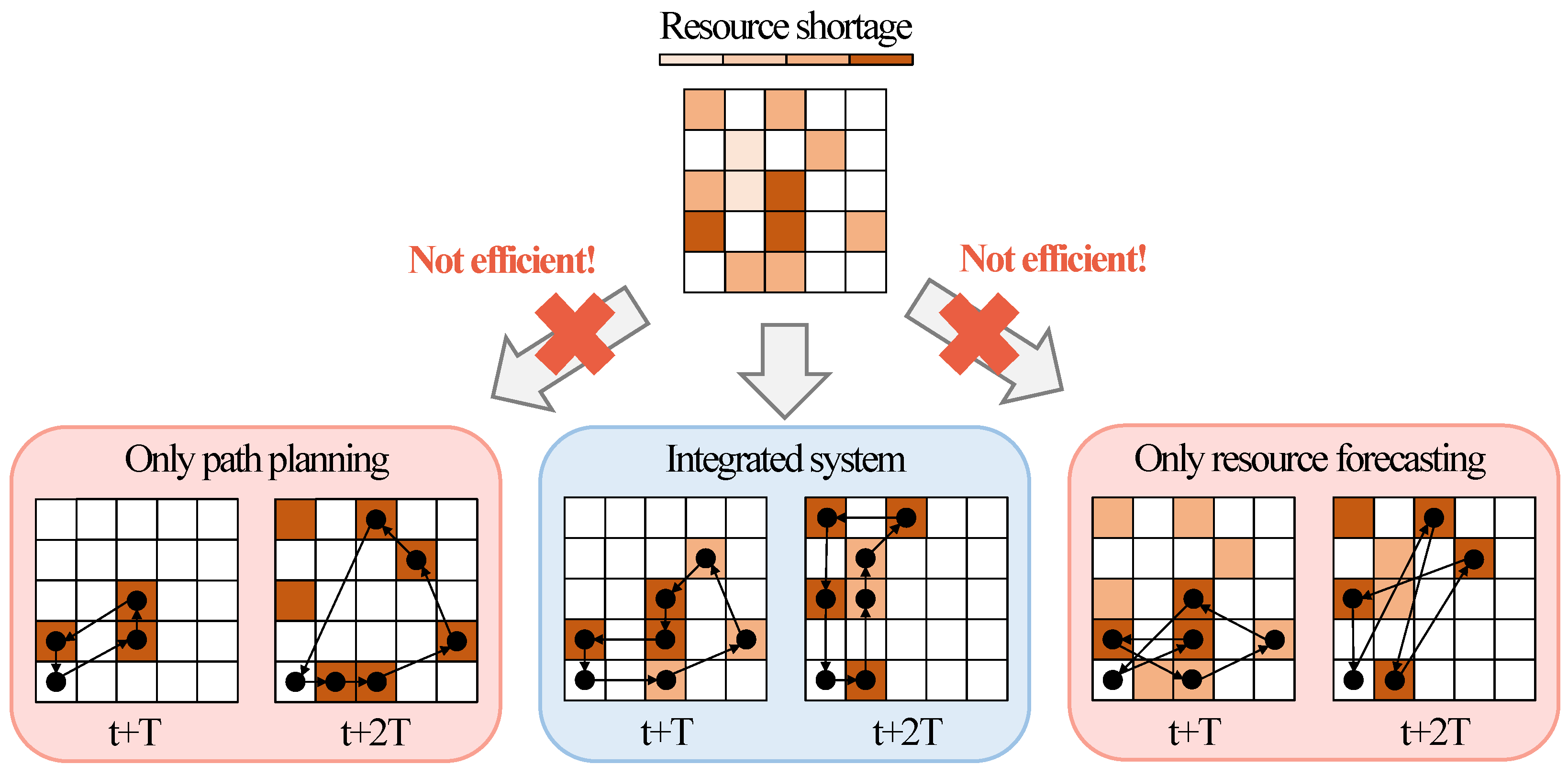
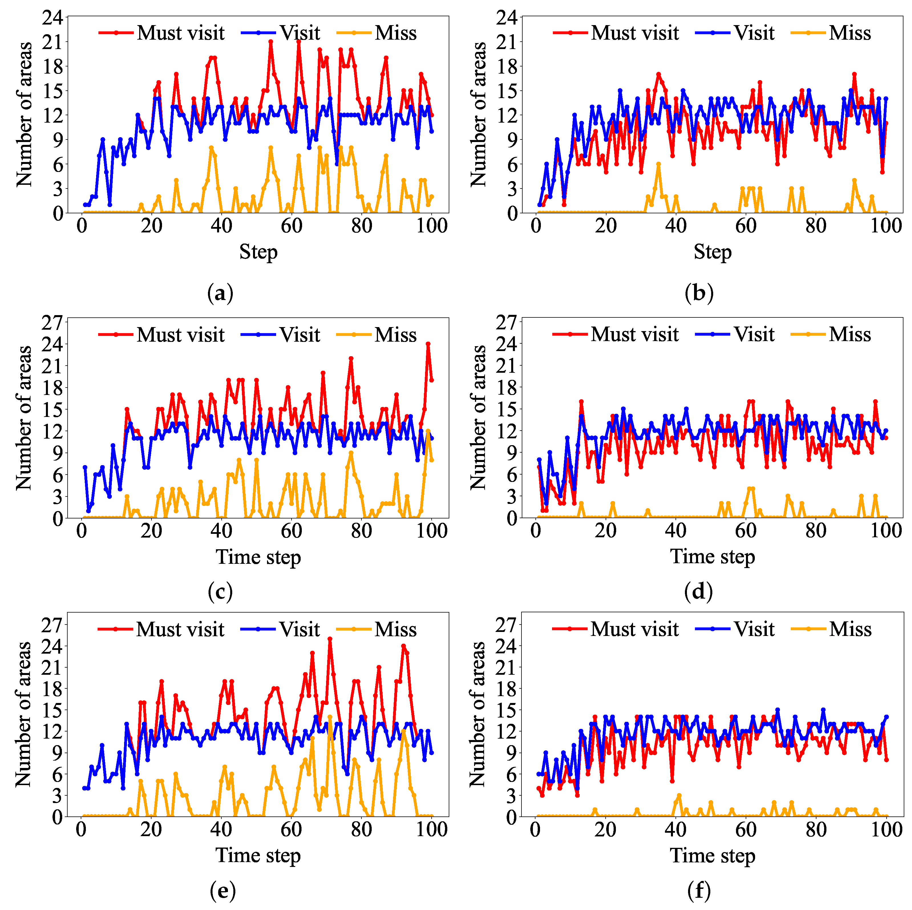
When only one of the two methods, path planning or resource forecasting, is applied in real environments, situations such as the one illustrated in Figure 1 may occur. When applying a path planning method, more areas can be covered under operational constraints. However, the number of required areas varies over time, being low during certain times and concentrated at specific times, with multiple areas requiring visitation simultaneously. If multiple areas that require visitation at the same time, it may be impossible to visit all areas due to operational constraints. Conversely, resource forecasting allows the UAV to utilize residual capacity after visiting required areas to handle additional areas in advance, thereby reducing future concentration of areas that require visitation. Nevertheless, due to inefficient movement in path planning, it may be impossible to visit a large number of areas. To address this issue, resource forecasting is used to prioritize areas for visitation, and a path planning method is applied to maximize the number of high-priority areas visited. This approach ensures that high-priority areas are visited as needed, improving overall mission efficiency.
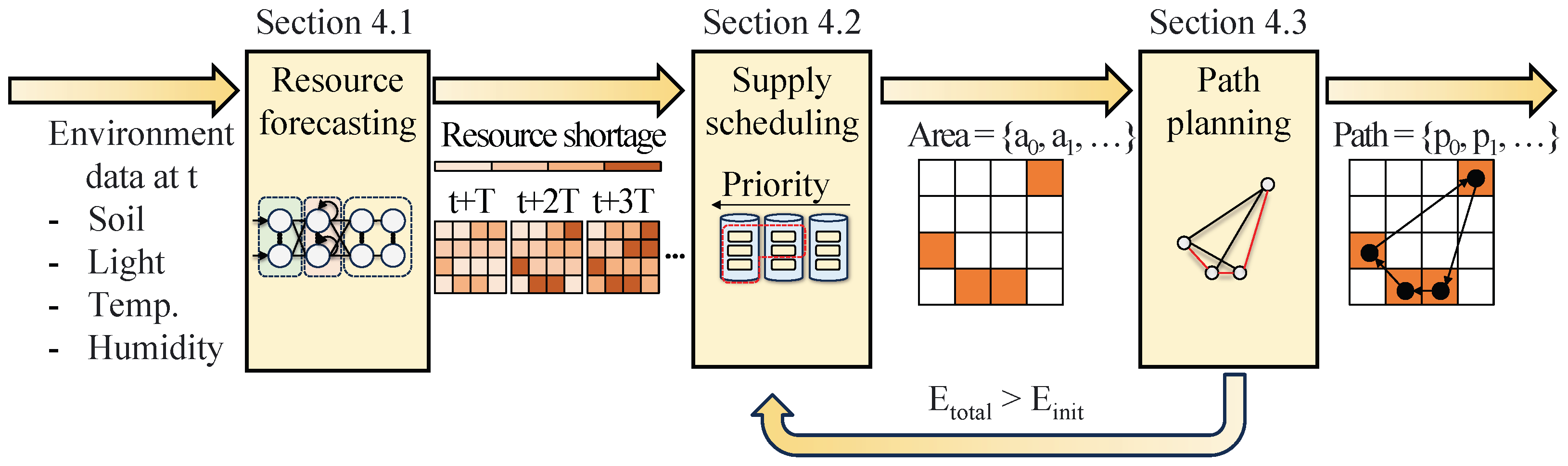
In this paper, we propose an integrated resource supply framework that forecasts future resources such as soil moisture using an RNN model, schedules the resource supply according to forecast-based priority, and derives the dynamic energy-aware UAV path to support. Figure 2 illustrates the proposed integrated smart farm framework. First, various environmental data such as soil moisture, light intensity, temperature, and humidity are collected at interval T. Using the collected data, an RNN model forecasts temporal patterns of potential water shortages in each area. Details of the model are discussed in Section 4.1. Once potential resource shortages in each area are identified, they are prioritized based on urgency—ranging from areas requiring immediate support to areas that will experience resource shortages in the near future. Based on this prioritization, the target areas to be supported by the UAV are determined. This is described in Section 4.2.
After determining the target areas for resource supply, we derive the UAV flight path required to visit those areas. To address this NP-hard Traveling Salesman Problem (TSP), we propose a hybrid heuristic algorithm that combines the Genetic Algorithm (GA) with the Christofides algorithm, thereby achieving efficient path planning within a short computation time. If the total energy consumption E t o t a l exceeds the UAV’s maximum allowable energy E i n i t , a rescheduling is performed to reduce the number of destinations. The detailed methodology for path planning is described in Section 4.3.
To evaluate the proposed system, we implemented the system shown in Figure 2, including resource forecasting, supply scheduling, and path planning. In this paper, we evaluate how effectively the proposed approach addresses resource shortage issues under different scheduling. For the open irrigation environment data, we confirmed that the proposed framework achieved an average reduction of 81.08% in the supply miss rate. The main contributions of this paper are summarized as follows:
  • Introduction to the integrated resource forecasting, scheduling, and path planning smart farm framework;
  • Implementation of an RNN-based resource forecast model using open environment data;
  • Development of the hybrid UAV path planning method for the resource supply under a given maximum energy;
  • Analysis of the impact of the proposed method on the resource supply result through simulation.
The remainder of this paper is organized as follows: Section 2 reviews existing smart farming operations, the UAV path planning method, the use of UAVs in agriculture, and studies that integrate prediction models into various systems. Section 3 introduces system models, such as the mobility model, the delay model, and the energy model. Section 4 introduces the RNN-based resource forecasting, supply scheduling method, and UAV path planning to maximize the number of resource shortage areas. Section 5 validates the proposed integrated smart farm framework. Finally, Section 6 concludes the paper and discusses potential future applications.

2. Related Work

Effective management methodology of water resources is becoming increasingly necessary in various fields with the increasing utilization of limited water resources [10]. In response to this need, machine learning-based smart irrigation systems have been conducted in recent years [11]. Some smart irrigation systems were proposed to determine whether irrigation is needed [12,13]. The systems in question have been integrated with IoT sensors where environmental data are gathered. Then, the data are classified based on similarity in characteristics. Based on the classification model, the operation of sprinklers or pumps is determined.
A comprehensive summary of the recurrent models, including their features and application fields, is provided in the review [14]. Table 1 summarizes the features and application fields of various recurrent models, such as RNN, Long Short-Term Memory (LSTM), and Gated Recurrent Unit (GRU), which are presented in [14].
Among the various application fields of recurrent models, some research has been conducted to forecast future soil moisture based on past environmental data that have been used for irrigation scheduling [5,6,7]. A LSTM model uses temperature, humidity, and soil moisture data as inputs and generates individual forecasts for each parameter [5]. The LSTM model and a scheduler were used for precise irrigation planning [6]. In addition, a research study proposed a deep bidirectional LSTM model to forecast soil moisture and electrical conductivity using IoT-sensed environmental data [7].
Such forecasts of soil moisture can be effectively integrated with UAV-based irrigation systems. However, due to the limited flight distance of UAVs, optimizing the UAV path is essential for efficient irrigation systems. In smart farming environments, UAVs are used for various purposes such as crop monitoring, pesticide spraying, and data collection. There are several research studies on UAV path optimization to solve the Coverage Path Planning (CPP) problem, which aims to design paths that enable UAVs to visit some points within the area of interest. One research study suggests the A * algorithm to optimize the UAV flight path for pesticide spraying [3]. Other researchers optimized the UAV flight path with a reinforcement learning method for collecting data measured by IoT sensors [8]. The method minimizes overlapping paths to cover the whole IoT devices. Furthermore, as an approach to solve the energy supply issues of IoT sensor nodes in a wide farm area, a path optimization system has been proposed that utilizes the UAV for wireless charging [9]. Some research studies tried to solve complex problems such as the fusion of TSP and CPP [15,16]. They redefined the path planning problem and used the Double Deep Q-Network to solve the problem. One research study proposed a task allocation and path optimization method for UAV operations in dynamically changing mission environments, incorporating energy constraints and cooperation among multiple UAVs [17]. In addition, another research study established a dynamic energy consumption model based on payload variation and derived the optimal UAV path using the heuristic search method [18].
Several research studies have also been actively conducted on integrating predictive models such as LSTM and RNN into systems to enhance overall efficiency. One research study proposed a dynamic UAV deployment algorithm that maximizes communication coverage by predicting ship trajectories using LSTM [19]. Another research study predicted the travel time between customers using LSTM and applied a hybrid GA to optimize delivery routes under real-time traffic conditions [20]. In addition, to address inefficiencies arising from the separation of procurement and production scheduling, an integrated planning method was proposed by combining LSTM-based procurement cost prediction with GA-based production scheduling optimization [21].
Although various studies have been conducted in the fields of resource forecasting and UAV path optimization, most research studies have only focused on individual fields. In addition, various studies have integrated prediction-based models with different applications to improve overall system efficiency. However, there have been few attempts that integrate both a method for forecasting the priority of resource supply areas and a UAV path planning method that considers both area priority and dynamic energy changes due to payload variation.

3. System Modeling

In this section, we describe the system model. Section 3.1 describes the mobility model based on UAV operations. Section 3.2 describes the delay model, which presents the UAV operation time in various operation modes. Section 3.3 describes the energy consumption model based on UAV operations and payload.

3.1. Mobility Model

Figure 3 illustrates the UAV mobility model assumed in this work. The UAV takes off from the station carrying resources for supply missions. It then flies to area 1, which requires resource supplies, and upon arrival, performs hovering to supply the resources. This process continues as the UAV visits multiple areas, and once all reachable areas within the flight constraints are visited, the UAV returns to the station and lands. The UAV mobility model includes take-off F t a k e , landing F l a n d , horizontal flight F i , m o v , hovering F i , h o v . F t a k e is defined by the flight altitude and take-off velocity, while F l a n d is defined by the flight altitude and landing velocity. F i , m o v is defined by the starting and destination point, flight distance, and flight velocity, while F i , h o v is defined by the UAV hovering time t i , h o v . The UAV’s total movement F is defined as follows:
F = F t a k e , F 1 , m o v , F 1 , h o v , F 2 , m o v , F 2 , h o v , , F N s u p + 1 , m o v , F l a n d
where F consists of F t a k e , F i , m o v , F i , h o v , and F l a n d . N s u p denotes the number of areas visited by the UAV for resource supplying. For example, if there are N s u p areas to visit, hovering is performed N s u p times. However, in the case of flight, it includes the return to the station, thus covering up to F N s u p + 1 , m o v .

3.2. Delay Model

Each UAV operation described in Section 3.1 involves a specific operation time t O P , which plays a critical role not only in calculating power and energy consumption but also in scenarios where the UAV must complete its mission within a limited time. In this work, the operation times for take-off t t a k e , landing t l a n d , and the UAV turning time t i , t u r n —if the UAV changes direction instead of flying in a straight line—are treated as constants. The flight time of the UAV t i , m o v can be calculated by dividing the flight distance by the flight velocity. The hovering time t i , h o v is defined as the sum of the resource supply time t i , s u p and any additional operation time, such as turning. In this work, t i , h o v is defined as the sum of t i , s u p and t i , t u r n , where t i , s u p can be calculated by dividing the amount of resources to be supplied by the supply speed. For example, if the sprinkler supplies resources at a rate of 0.5 L/s and performs a 1 s for turning, the UAV must hover for 11 s to supply 5 L of resources and complete the turning. The UAV’s flight time in each step t t o t a l is defined as follows:
t t o t a l = t t a k e + i = 1 N s u p + 1 t i , m o v + i = 1 N s u p t i , h o v + t l a n d , t i , h o v = t i , s u p + t i , t u r n .

3.3. Energy Model

To plan UAV flight paths, it is necessary to consider dynamic energy consumption that varies with factors such as operation mode, speed, and payload and to derive a flyable path within the constraints of limited battery capacity. In particular, when UAVs are required to perform specific tasks such as delivery or resource supply in addition to simple movement, considering dynamic energy consumption becomes even more critical. Therefore, it is essential to accurately model UAV power, energy, and battery consumption. The motor power P m o t o r is determined by the UAV’s physical characteristics, payload, velocity, acceleration, and operation mode. In this work, assuming that the UAV maintains a constant velocity with the same UAV model, P m o t o r is primarily determined by the payload and operation mode.
For each operation mode, the power P O P and energy E O P are defined as follows:
P O P = P m o t o r × N m o t o r
E O P = P O P × t O P
where the value of P m o t o r varies depending on the UAV’s operation mode and payload, and accordingly, P O P and E O P are determined by the number of active motors N m o t o r , which yields t O P . When the UAV sequentially visits multiple areas, supply resources, and returns, the total energy consumption E t o t a l is defined as follows:
E t o t a l = E t a k e + i = 1 N s u p + 1 E i , m o v + i = 1 N s u p E i , h o v + E l a n d
where E i , h o v and E i , m o v vary depending on the payload. The hovering time of the UAV at the i-th supply area, required to compute E i , h o v , is determined by t i , s u p and t i , t u r n . For example, if the UAV starts its resource supply mission with a payload of 5 kg, then E 1 , m o v and E 1 , h o v represent the total energy consumption for flight and hovering with the 5 kg payload during the first movement to a supply area. As the UAV visits each area and supplies resources, the payload decreases, and therefore, its energy and battery consumption can differ even for the same operation mode depending on the point in time. In this work, the UAV take-off and landing only once, so the corresponding energy for take-off and landing are calculated based on the payload at those moments. However, if take-off and landing occur multiple times, they should be computed similarly to hovering and flight operations. This payload-based dynamic energy modeling enables significantly more precise path planning than simple distance-based or static energy models and is essential for designing realistic flight paths that UAVs can actually execute.

4. Resource Supply Planning

In this section, we propose an integrated method for resource supply planning. Section 4.1 describes the RNN-based resource forecast model. This model forecasts the future resource trend from recent environmental information. The forecast results are used for supply scheduling. Section 4.2 describes how to plan the the order of the supply based on the resource forecast. Based on the forecast results, resource supplying is scheduled with priority given to areas with low current resources or areas where resources are depleting quickly. Section 4.3 presents the path planning method for supplying the scheduled areas. If E t o t a l is larger than E i n i t , the supply plan must be adjusted accordingly.

4.1. RNN-Based Resource Forecasting

Soil moisture, one of the important resources for agriculture, is determined by various parameters, such as air temperature, air humidity, and light intensity [22]. Forecasting the trend of this key resource is essential for improving irrigation efficiency, and it requires past environmental data over a specific period. The required environmental data take the form of sequence data, specifically time-series data. Sequence data are highly correlated with both current and previous states, and due to this characteristic, they are difficult to model using standard feedforward networks. In contrast, RNNs include hidden layers that extract features, allowing them to perform better in modeling sequence data compared to standard feedforward networks [23]. The RNN-based Sequence-to-Sequence model is widely applied in various fields, such as machine translation, text summarization, headline generation, and sequence data analysis [24].
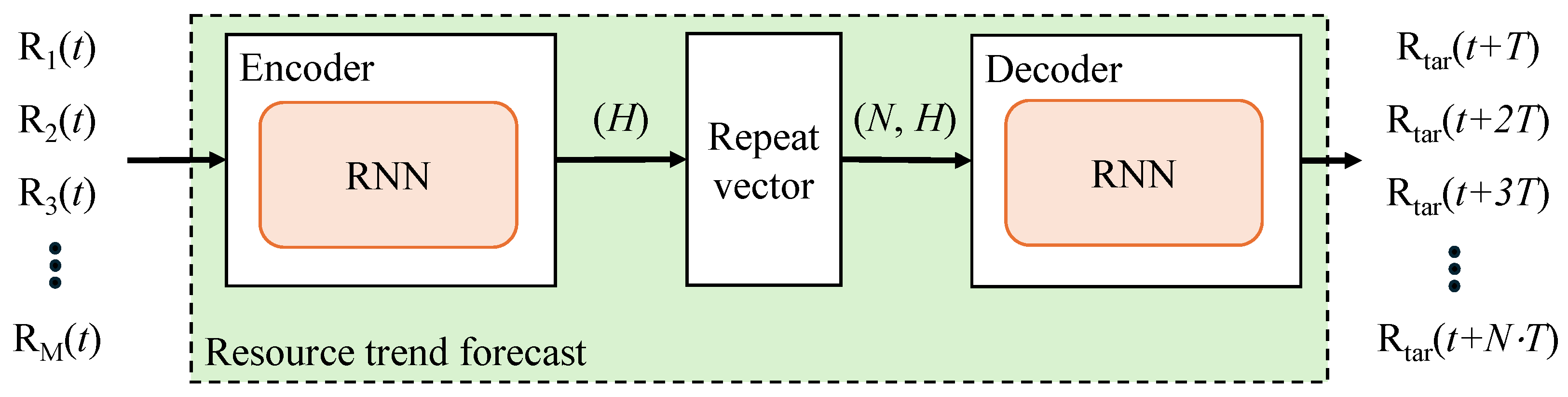
Figure 4 illustrates the model for forecasting resource trends R t a r ( t + i ) . M and N represents the number of inputs and outputs of the model, respectively. The inputs of the model are R 1 ( t ) to R M ( t ) at time t, and the outputs of the model are R t a r ( t + T ) to R t a r ( t + N · T ) , where T means the period for the forecast. These inputs take the form of sequential data, and the encoder compresses them to represent the features of the data. These data are used by the decoder for forecasting. The output of the encoder, which has a hidden state size H, is transformed into a shape of ( N , H ) using a repeat vector. This operation replicates the encoder output into N copies, because the decoder requires N inputs, whereas the encoder generates only one output. The decoder transforms the compressed data into different sequence data, allowing R t a r forecast from t + T to t + N · T . These outputs are used as inputs for resource supply scheduling in Section 4.2. During training, the model learns to minimize the mean squared error between the forecasted outputs and the actual values. The entire model is trained end-to-end using Backpropagation Through Time, and detailed hyperparameter settings are described in Section 5.2.
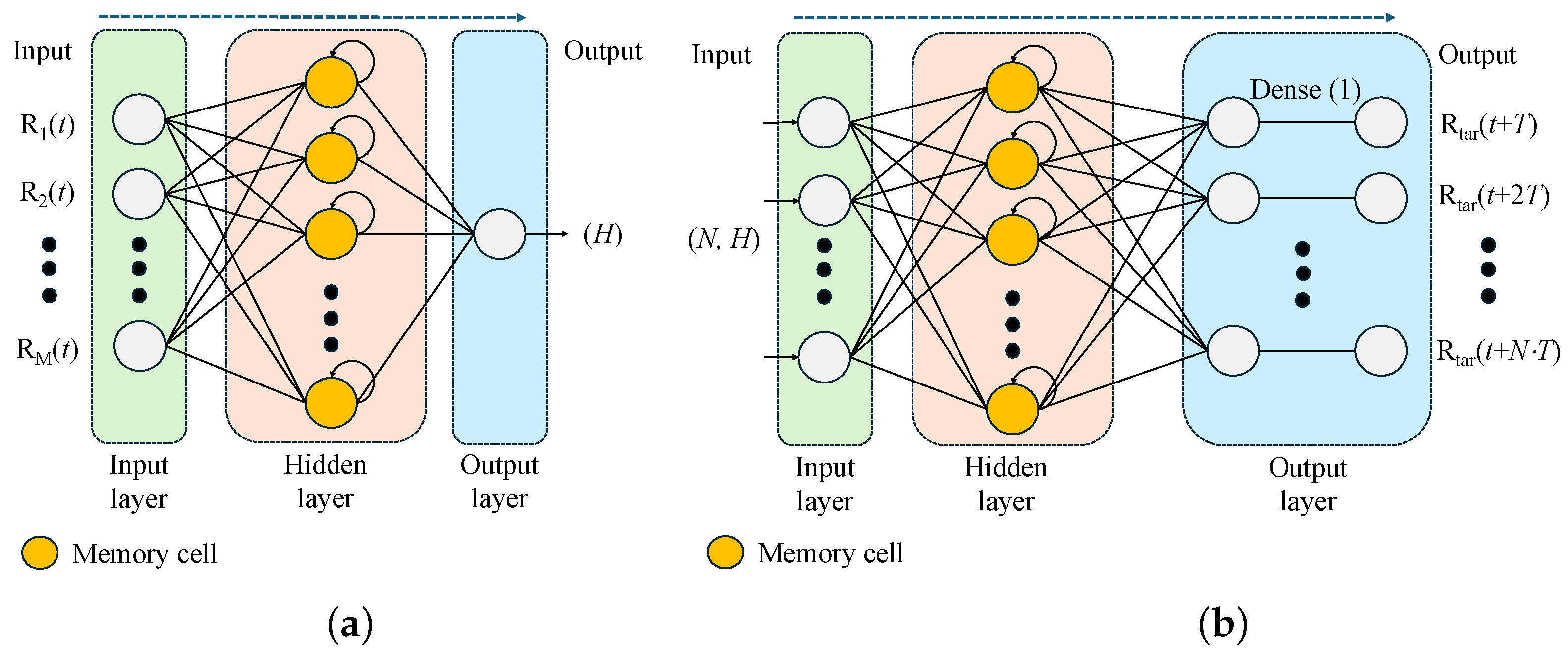
Figure 5 illustrates the RNN structures of the encoder and decoder, respectively. As illustrated in Figure 5a, the encoder receives M inputs and generates one output, which has a hidden state size of H. As illustrated in Figure 5b, the decoder receives N inputs replicated by the repeat vector and generates N outputs. The hidden layers of both the encoder and decoder consist of memory cells, where each cell generates an output based on the current input and hidden state. The hidden state is the output generated from the previous input and is a compressed summary of all the data from previous inputs. As illustrated in Figure 4, the proposed model generates output using N steps of input data. Therefore, the hidden layers of both the encoder and the decoder perform N iterations of computation before producing the final output. The use of memory cells in both the encoder and decoder plays a critical role in preserving and leveraging temporal dependencies. In particular, the final hidden state of the encoder acts as a compact summary of the dynamic information from the input time series, which the decoder then expands to generate predictions over multiple future time steps. This memory-based architecture is essential for capturing temporal trends in resource data and serves as a foundational component of the proposed resource operation planning system.

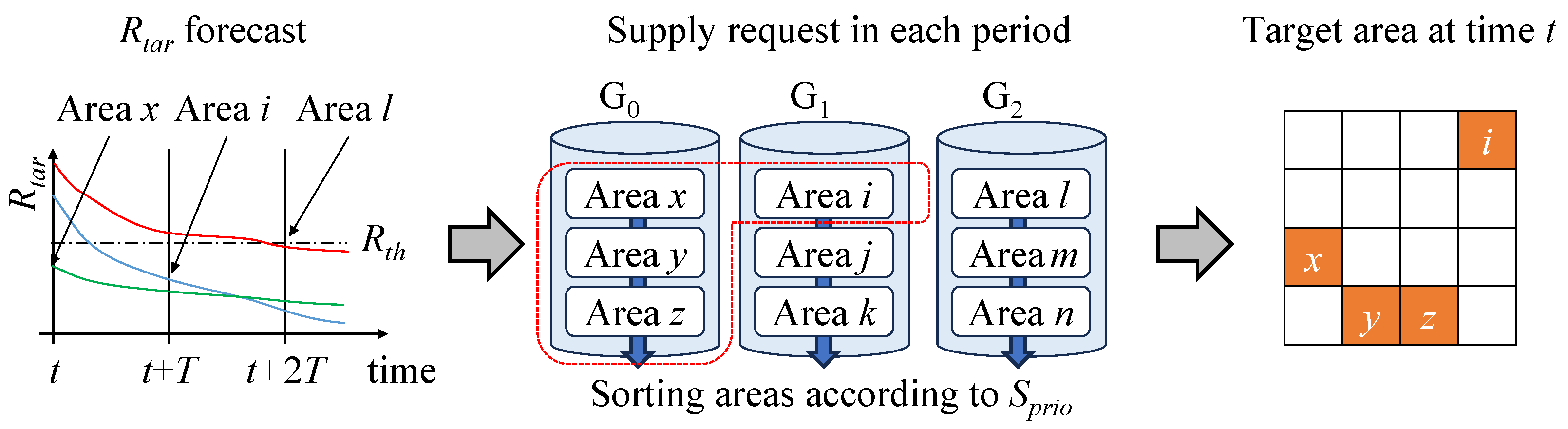
4.2. Supply Scheduling

Resource supply scheduling plays a key role in efficient resource management. Based on the forecasted data of resources, R t a r in Section 4.1, we proposes a resource supply scheduling method based on forecasted data.
Figure 6 illustrates the proposed supply scheduling process, which is performed according to the follow steps. First, based on the resource forecast model, we obtain the measured resource data R t a r ( t ) and forecasted resource data R t a r ( t + i · T ) . In this case, R t a r is normalized between 0 and 1. Then, we detect the time at which R t a r drops below the resource threshold R t h . Based on each detected time step T, each area is assigned to one of the groups G 0 , G 1 , , G N . For example, R t a r ( t ) at area x is lower than R t h . So, area x is assigned to G 0 . Also, area i is assigned to G 1 because the R t a r ( t + T ) of area i is lower than the R t h .
In the next step, within each group, areas are sorted according to a given priority score S p r i o ( t + i · T ) at time t + i · T , which is derived as
S p r i o ( t + i · T ) = ( 1 R t a r ( t + i · T ) ) + α × S g r a d ( t + i · T ) .
For the first term 1 R t a r ( t + i · T ) , fewer resources mean higher priorities. S g r a d ( t + i · T ) is the gradient score at time t + i · T that indicates the degree of variability in the forecasted data. A higher S g r a d ( t + i · T ) means a rapid decline in R t a r ( t + i · T ) . α is the adjustment coefficient. A smaller α focuses more on R t a r ( t + i · T ) shortage, whereas a larger α gives more weight to the trend of R t a r ( t + i · T ) . S g r a d is specified as
S g r a d ( t + i · T ) = k = i N + i 1 ( R t a r ( t + ( k + 1 ) · T ) R t a r ( t + k · T ) ) × 1 k
where R t a r ( t + k · T + 1 ) R t a r ( t + k · T ) means the variation of R t a r at time t + k · T . By setting the weight to 1 k , sudden fluctuations in the near future are more strongly reflected in S g r a d ( t + i · T ) .
After sorting the areas based on S p r i o ( t + i · T ) in each group, we select the target areas to be supported by the UAV at time t. First, select the area in the group with the smaller i value, and then select in order of priority if the area is in the same group. The number of areas that can be selected depends on the flight distance of the UAV. If the UAV maximum flight distance is long enough, more areas can be supplied via the UAV. However, if the UAV flight path, which will be covered in the next section, is not sufficiently optimized, the number of areas is limited.
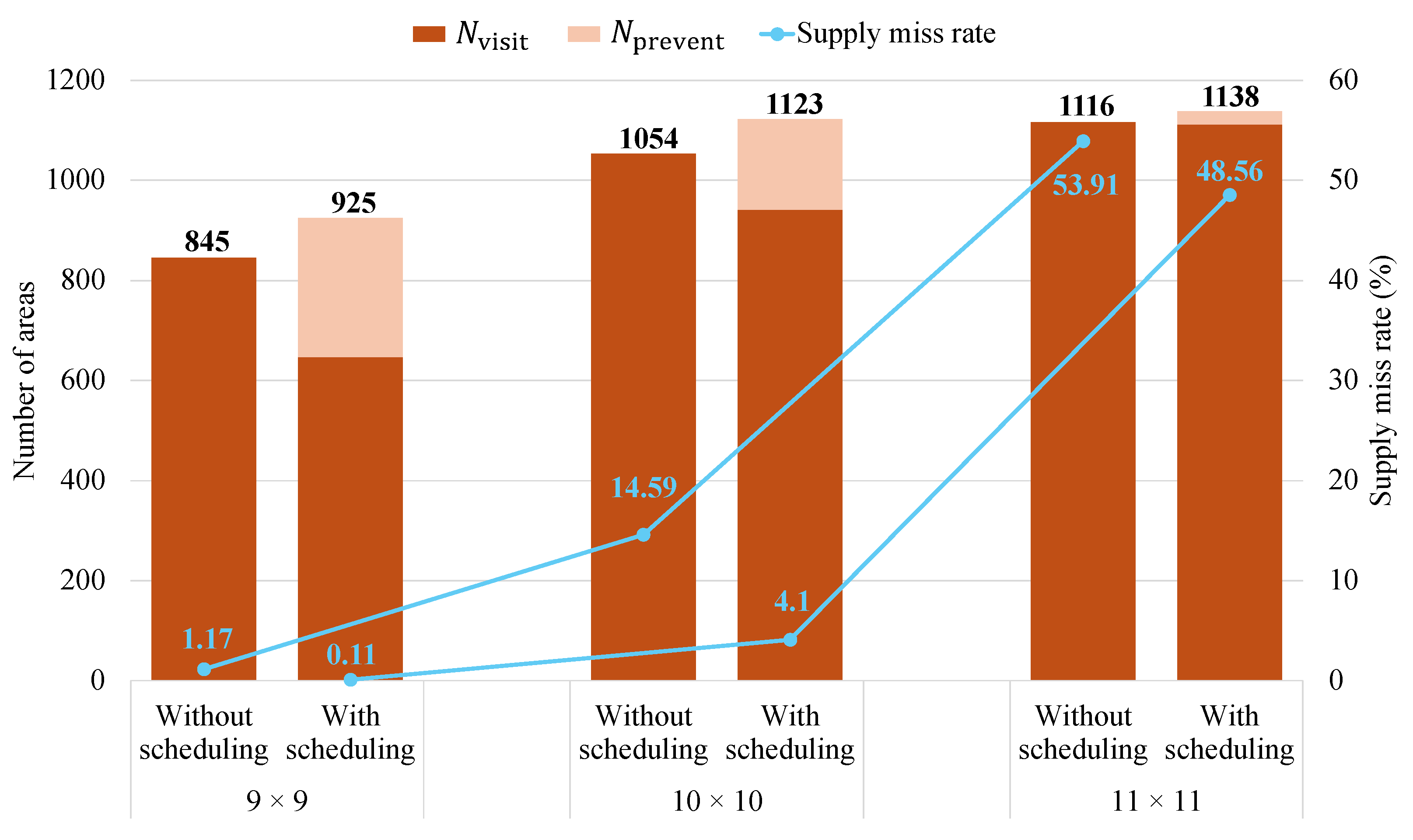
We introduce some terms to evaluate the supply miss rate as a metric. The number of required resource supply areas visited by the UAVs is N v i s i t , and the number of areas visited before resource shortage occurs is N p r e v e n t . The number of areas requiring resource supply is N s h o r t a g e , and the supply misses is N m i s s = N s h o r t a g e N v i s i t . The areas that are not supported remains in G 0 and are given the highest supply priority in the next round t + T . To evaluate the performance of the resource supply system, we define the supply miss rate as follows:
Supply miss rate = i = 1 K N m i s s ( t + i · T ) i = 1 K N s h o r t a g e ( t + i · T ) + i = 1 K N p r e v e n t ( t + i · T ) × 100
where the supply miss rate represents the total number of supply misses of the total number of shortages over the total K times of supply.

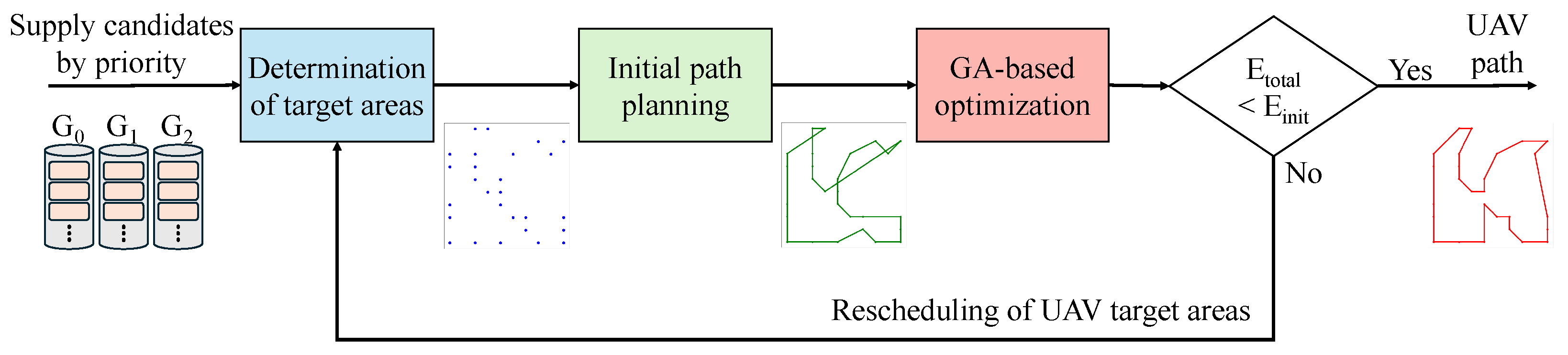
4.3. UAV Path Planning

In various applications of UAVs, their limited flight distance acts as a significant constraint. To overcome this limitation, the battery capacity can be expanded; however, the resulting increase in battery weight causes higher power consumption during UAV flight. Our objective is solve this problem by deriving the UAV flight path that considers both visit priorities and dynamic energy consumption in order to visit the target areas. To address this, we propose a hybrid heuristic algorithm that combines the Christofides algorithm with the GA.
Figure 7 illustrates the path planning process applying the proposed hybrid heuristic algorithm. First, target areas are determined through the resource supply scheduling method. Then, an initial solution for visiting these target areas is derived by applying the Christofides algorithm. The Christofides algorithm is an algorithm for deriving an approximate solution to the TSP, providing an approximation with a guaranteed performance bound [25]. However, since it does not always guarantee the optimal solution, the solution to the Christofides algorithm is used as the initial path for the proposed UAV path planner.
The GA is a metaheuristic algorithm based on the concept of genetic evolution, which explores a diverse set of solutions through genetic operations such as selection, crossover, and mutation [26]. In this work, path planning is performed in each iteration by applying crossover, mutation, and selection to solutions selected based on either the initial path or the one with the lowest E t o t a l . If the E t o t a l of the path derived by the proposed path planning method exceeds E i n i t , the target areas for resource supply are rescheduled. The proposed hybrid heuristic algorithm addresses the approximation limitations of the Christofides algorithm while reducing the computation time of the GA.
Algorithm 1 shows the proposed resource-forecasting-based path planning method. The inputs of the method are the area groups G 0 , G 1 , …, G N , which are classified based on priority in Section 4.2, and E i n i t . The output of method is a UAV flight path that considers both the priority of the areas and dynamic energy consumption. First, the areas in two highest-priority groups are assigned to A r e a m u s t , while the remaining areas are assigned to A r e a e x t r a (lines 4–5). Subsequently, the Christofides algorithm is applied to generate an initial approximate optimal path P a t h i n i t that visits the A r e a m u s t (line 6). If the value of I is 1, the P a t h i n i t is refined using genetic operations, including mutation, crossover, and selection, to initialize P a t h b e s t . The S b e s t for this path is calculated based on the number of visited areas and energy efficiency metric, which is the total energy consumption divided by the number of visited areas (lines 9–10). If I is not 1, the proposed algorithm iteratively explores paths based on N c o m b , which is the number of combinations within A r e a e x t r a (line 12). A subset of areas from A r e a e x t r a is added to P a t h b e s t to expand the path, followed by genetic operations. The E t o t a l of the temporary path P t e m p is calculated using Equation (5). If the P a t h t e m p satisfies the energy constraint and S t e m p exceeds S b e s t , then both P a t h b e s t and S b e s t are updated (lines 13–18). If E t o t a l exceeds E i n i t , meaning the UAV cannot execute the path, the areas in A r e a m u s t and A r e a e x t r a are reconfigured to reschedule the visiting area set and explore the path (lines 19–21). If even the areas in G 0 cannot be visited within the energy constraints, the proposed algorithm attempts to find an available combination of areas from G 0 that satisfies the energy constraints. The overall time complexity of the Algorithm 1 depends on three main factors: I, N c o m b , and the total number of candidate areas N t o t a l . Genetic operations and energy evaluations are performed on each candidate path. In the worst case, each path may include up to N t o t a l points; the proposed Algorithm 1 has a time complexity of O ( I · N c o m b · N t o t a l ) .
Algorithm 1: Resource-forecasting-based path planning method
  1:
Input:  G 0 , G 1 , …, G N , E i n i t
  2:
Output:  P a t h b e s t
  3:
P a t h b e s t { } , P a t h i n i t { } , P a t h t e m p { }
  4:
A r e a m u s t G 0 , G 1
  5:
A r e a e x t r a G 2 , G 3 , , G N
  6:
P a t h i n i t Christofides Algorithm ( A r e a m u s t )
  7:
for I iterations do
  8:
   if I == 1 then
  9:
      P a t h b e s t mutation ( P a t h i n i t ) , crossover ( P a t h i n i t ) , selection ( P a t h i n i t )
10:
      S b e s t evaluate ( P a t h b e s t )
11:
   else
12:
     for  N c o m b iterations do
13:
         P a t h b e s t P a t h b e s t + subset ( A r e a e x t r a )
14:
         P a t h t e m p mutation ( P a t h b e s t ) , crossover ( P a t h b e s t ) , selection ( P a t h b e s t )
15:
         S t e m p evaluate ( P a t h t e m p )
16:
        if  E t o t a l < E i n i t S t e m p > S b e s t  then
17:
           P a t h b e s t P a t h t e m p
18:
           S b e s t S t e m p
19:
        else if  E t o t a l > E i n i t   then
20:
           A r e a m u s t G 0
21:
           A r e a e x t r a G 1 , G 2 , , G N
22:
        end if
23:
     end for
24:
   end if
25:
end for
While static energy models are relatively easy to apply because they can be modeled in advance of the path planning, dynamic energy models are more challenging to incorporate in standard GAs, as energy consumption continuously changes depending on the UAV’s flight path. To address this limitation, the proposed method applies the dynamic energy model to each candidate path during evaluation to determine its feasibility and iteratively improves the path using selection, crossover, and mutation operations. However, this approach requires recalculating the energy consumption for every candidate route, leading to a significant increase in computational load as the number of target areas increases. To address this issue, the proposed hybrid algorithm initializes the search with a near-optimal path generated based on flight distance, thereby reducing the number of iterations and effectively narrowing the search space. As a result, it can significantly reduce the computation time while still ensuring a satisfactory level of path quality compared to the GA-based path planning method that begins with random paths.

5. Validation

This section evaluates the performance of the proposed integrated smart farm framework. Section 5.1 describes the resource forecasting model and validation setup for evaluating the proposed integrated framework. Section 5.2 evaluates the performance of the proposed resource forecasting model. Section 5.3 evaluates the resource supply efficiency of the proposed integrated framework under three different simulation environments.

5.1. Validation Setup

In this work, we used an RNN-based resource forecasting model, illustrated in Figure 4, to forecast soil moisture S M trends. To train and validate the proposed resource forecasting model and integrated smart farm framework, we used an experimental dataset related to wheat provided by SMART FASAL (https://smartfasal.in/ (accessed on 16 July 2025)). This dataset consists of the key resource, SM, as well as temperature, humidity, light intensity, and atmospheric pressure data measured at 15-minute intervals from 3 March 2021 to 16 April 2021. A detailed explanation of the dataset, hyperparameter settings, and the proposed resource forecasting model are provided in Section 5.2.
To model the energy consumption for take-off, landing, hovering, and flight with consideration of the payload, the UAV’s specifications and experimental results from [27] were used. Table 2 summarizes the specifications of the UAV, which are reported in [27]. Assuming a maximum payload of 10 kg, the energy consumption is modeled as a function of the payload mass—based on both data from [27] and the functional form presented in [28]. In this work, the energy consumption is calculated based on the energy required to move 1 m under different payload conditions. Since the UAV is assumed to move at a constant speed of 1 m/s, the time to flight for 1 m is 1 s. Therefore, the energy consumption values are equivalent to the power values, as the energy is computed as power multiplied by time. Table 3 and Figure 8 illustrate the energy consumption of each UAV operation mode according to payload. As the payload increases, the energy consumption also increases, showing a steeper rise for heavier payloads. In particular, the energy consumption for take-off and hovering increases more significantly as the payload becomes heavier.
To evaluate the performance of the proposed integrated framework, the following simulation was performed three times, with each performed in a different environment. Each environment consisted of 100 areas, and the characteristics of each area were defined based on the dataset to train the resource forecasting model. Each dataset was initialized independently and used for resource forecasting, resource supply scheduling, and UAV path planning. Each area was designated as requiring irrigation when its normalized resource value was less than 0.465. Figure 9 illustrates the three different simulation environments. Each environment has a different S M distribution, and darker areas indicate lower S M values, while brighter areas indicate higher S M values. Each area is defined as 17 m × 17 m in size, derived from the spray-width calculation method in [29] with a flight altitude of 6 m, resulting in a total simulation environment of 170 m × 170 m. The UAV starts from (0,0), visits all reachable areas, and finally returns to (0,0) after completing the resource supply mission. The UAV is assumed to carry 10 kg of water at the start of each mission and supplies 0.5 kg of water to each area it visits. The t s u p is 25 s for water supply, t t u r n is 1 s, and flies at a constant speed of 1 m/s. Both t t a k e and t l a n d are assumed to be 10 s each. In each simulation, each time supply occurs, the S M value of the area is re-initialized to a random normalized value, which subsequently decreases according to the area’s modeled trend.

5.2. Resource Forecasting Results

In this work, the RNN was chosen considering its ability to learn from relatively small datasets and its advantage in training and inference speed compared to LSTM [30,31]. The RNN-based forecasting model used in this work is composed of an encoder–decoder structure, where both the encoder and decoder include an RNN layer with 64 hidden units. The model was trained using the Adam optimizer with a mean squared error loss function for 300 epochs and a batch size of 32. As mentioned in Section 5.1, we used a publicly available dataset to train the model for forecasting S M in this work. Since this dataset only reflects decreasing S M trends, we augmented the training data by duplicating and appending arbitrary segments of the time series. This allowed the model to learn and forecast S M behavior following resource supply. The input data measured over 15-minute intervals were resampled at 3-hour intervals and used for training. Following the resampling process, a total of 1396 training samples were generated by constructing input–output pairs using a sliding window. The training samples were split into 80% for model training and 20% for evaluation. M was set to 4 as S M , temperature, humidity, and light intensity. T was set to 3 h, and N was set to 4 to forecast the next 12 h of S M based on the previous 12 h of input data. All S M values were normalized for both training and evaluation. Before normalization, the maximum and minimum S M values were 1406.65 and 0, respectively.
Table 4 compares the performance of the LSTM and RNN-based resource forecasting models evaluated on the test dataset. Since the LSTM model generally requires more training, 500 and 300 epochs were used to train the LSTM and RNN models, respectively. The performance was evaluated based on the Mean Absolute Error (MAE), Root Mean Squared Error (RMSE), Coefficient of Determination ( R 2 ), training time, and inference time metrics. The MAE measures the average magnitude of errors by computing the absolute errors, thereby directly representing error magnitudes. The MAE values of the LSTM and RNN models were 0.0092 and 0.0142. respectively, indicating that the both models presented small average forecasting error. The RMSE, which is more sensitive to larger errors, was 0.0283 for the RNN model and 0.0390 for the LSTM model, indicating that both models maintained low overall forecasting errors. In terms of R 2 , which measures how well the model captures the underlying data patterns, the RNN achieved a slightly higher value of 0.9838 compared to 0.9693 for the LSTM, demonstrating that the RNN performed comparably despite its simpler structure and faster computation. This performance was sufficient for use in the resource supply simulation performed in this work. Therefore, we adopted the RNN-based model for resource forecasting.

5.3. Resource Supply Result

To evaluate whether the proposed integrated system combining the scheduling method and path planning method could effectively reduce the supply miss rate, as described in Section 4.2 as a performance metric, UAV-based resource supply simulations were performed to compare the following two methods: (1) path planning without a scheduling method, and (2) the proposed path planning with a scheduling method. In this work, we defined a path planning as a method that generates an approximate optimal path using the Christofides algorithm and uses it as the initial path for the GA. For the both path planning methods, 500 iterations were performed per execution. However, the execution process may be repeated multiple times if the derived path fails to meet the feasibility constraints. In such cases, the supply-required areas are modified, and path planning is re-executed accordingly. Both of the path planning methods were configured with a population size of 50, a mutation rate of 0.015, a tournament selection size of 5, crossover applied at every iteration, and elitism enabled. In the path planning with the scheduling method, the adjustment coefficient α used for scheduling was set to 1. In the path planning without a scheduling method, the UAV only supported the resource shortage areas at each time step, where each time step corresponded to the predefined T defined in Section 5.2. All simulations were performed over 100 time steps.
Figure 10 illustrates the simulation results under different scenarios. Must visit, Visit, and Miss correspond to N s h o r t a g e , N p r e v e n t + N v i s i t , and N m i s s , respectively, at each time step. In the path planning without a scheduling method, it can be observed that as the N s h o r t a g e increased, the N m i s s also accumulated. Consequently, as the simulation progressed, the path planning without a scheduling method failed to cover all N s h o r t a g e . The proposed path planning with the scheduling method supplied near-shortages as well as shortages according to priority. This forecast-based scheduling reduced large numbers of future shortages, and it effectively reduced N m i s s by covering a larger number of areas while preventing the concentration of areas requiring resource supply at specific time steps.
Figure 11 and Figure 12 illustrate the path planning results in scenario 1 at different time steps. Each figure illustrates the required areas (dark brown), which need resource supply at the current time step, and the optional areas (light brown), which are predicted to require resources in the near future and are proactively visited in advance at the current time step. The green area represents the UAV’s base station for take-off and landing with resources, and the gray areas indicate consistently invalid areas located outside the 10 × 10 environment grid. As shown in Figure 11, when the number of required area was small, the path planning without a scheduling method could visit most required areas. However, the required areas were concentrated in a specific time step, and the UAV failed to visit all the required areas. In contrast, as shown in Figure 12, the path planning with the scheduling method distributed the visits in advance, effectively reducing the number of required areas at each time step. This enabled the UAV to supply resources to more areas at the appropriate time.
Table 5 summarizes the simulation results in each scenario, with the lowest supply miss rate in each case highlighted in bold and underlined, where we define N a r e a as the sum of N v i s i t and N p r e v e n t . The proposed path planning with the scheduling method achieved the lowest supply miss rate across all scenarios. D a v g and E a v g are calculated by dividing the total flight distance and total energy consumed over 100 time steps by the number of areas visited during those steps N a r e a . In other words, they represent the distance and energy per visited area. Compared to the path planning without a scheduling method, the proposed path planning with the scheduling method achieved an average reduction of 81.08% in the supply miss rate. The proposed method also showed smaller values of D a v g and E a v g , indicating more efficient flight in visiting the areas.
Computation time refers to the total time required for path planning after scheduling. In the case of path planning without scheduling, the algorithm solves the problem at each time step without considering N c o m b to visit as many required areas as possible. On the other hand, path planning with scheduling involves generating a path that must include all required areas while also considering optional areas based on priority, which requires additional computation time. Specifically, it includes the additional time required to compute N c o m b . This corresponds to the computational complexity O ( I · N c o m b · N t o t a l ) described in Section 4.3.
To further compare the performance outcomes across various environment sizes, additional simulations were performed under the same conditions as scenario 1, with only the number of areas changed. The number of areas was reduced or increased by approximately 20%, resulting in grid sizes of 9 × 9 and 11 × 11, respectively, compared to the original 10 × 10 setup. The total environment area in these case is defined as 153 m × 153 m and 187 m × 187 m. Figure 13 illustrates the simulation results for different environment sizes. Without scheduling and With scheduling correspond to the path planning methods without and with scheduling, respectively. The numbers above the bars represent N a r e a , while the blue numbers represent the supply miss rate. As the environment size decreased, the supply miss rate was reduced for both methods, with the proposed method consistently achieving a lower supply miss rate. However, when the environment size increased, both methods showed a high supply miss rate due to the UAV’s limited allowable energy, which restricted its ability to fly and supply resources to the required areas. Nevertheless, the proposed method still achieved a lower miss rate than the method without scheduling.

6. Conclusions

In this paper, we proposed an integrated smart farming framework that combines AI-based resource forecasting and UAV-assisted resource supply to enhance operational efficiency. By leveraging the RNN, the system effectively forecasts resource shortages using time-series environmental data. Based on these forecasts, supply scheduling prioritizes areas with the highest urgency, and UAVs are deployed accordingly. To further optimize the resource supply process, we introduced a hybrid UAV path planning method, which maximizes the number of areas that receive resource supply. If the total energy consumption exceeds the UAV’s maximum allowable energy, the system reschedules the resource supply tasks to maintain feasibility. Experimental evaluation demonstrates that the proposed method improves the effectiveness of resource supply, confirming its applicability in real-world smart farming environments. Future work will focus on utilizing multiple UAVs to enhance the system’s applicability in real-world environments. Also, we will aim to solve other problems, such as UAV operational constraints in adverse weather, UAV collision probability, and robustness to sensor failure, using deep reinforcement learning.

Author Contributions

Conceptualization, D.Y. and D.B.; methodology, D.Y.; validation, D.Y.; writing—original draft preparation, D.Y.; writing—review and editing, D.B. and Y.C.; supervision, D.B. All authors have read and agreed to the published version of the manuscript.

Funding

This research was supported by the Basic Science Research Program through the National Research Foundation of Korea (NRF) funded by the Ministry of Education (RS-2020-NR049604) and the Chungbuk National University BK21 program (2023).

Data Availability Statement

The original contributions presented in this study are included in the article.

Conflicts of Interest

The authors declare no conflicts of interest.

References

  1. Santiteerakul, S.; Sopadang, A.; Yaibuathet Tippayawong, K.; Tamvimol, K. The Role of Smart Technology in Sustainable Agriculture: A Case Study of Wangree Plant Factory. Sustainability 2020, 12, 4640. [Google Scholar] [CrossRef]
  2. Mat, I.; Mohd Kassim, M.R.; Harun, A.N.; Yusoff, I.M. Smart Agriculture Using Internet of Things. In Proceedings of the 2018 IEEE Conference on Open Systems (ICOS), Langkawi, Malaysia, 21–22 November 2018. [Google Scholar]
  3. Baidya, K.; Dampella, A.J.R.; Surya Charan Paidipalli, V.V.; Bansod, S.; Singh, S.K.; Pal, P. Pesticides Spraying Using Non-GPS-Based Autonomous Drone. In Proceedings of the 2022 International Conference on Futuristic Technologies (INCOFT), Belgaum, India, 25–27 November 2022. [Google Scholar]
  4. SP, P.; Balamurugan, P. Unmanned Aerial Vehicle in the Smart Farming Systems: Types, Applications and Cyber-Security Threats. In Proceedings of the 2022 International Conference on Innovative Computing, Intelligent Communication and Smart Electrical Systems (ICSES), Chennai, India, 15–16 July 2022. [Google Scholar]
  5. Sami, M.; Khan, S.Q.; Khurram, M.; Farooq, M.U.; Anjum, R.; Aziz, S.; Qureshi, R.; Sadak, F. A Deep Learning-Based Sensor Modeling for Smart Irrigation System. Agronomy 2022, 12, 212. [Google Scholar] [CrossRef]
  6. Kashyap, P.K.; Kumar, S.; Jaiswal, A.; Prasad, M.; Gandomi, A.H. Towards Precision Agriculture: IoT-Enabled Intelligent Irrigation Systems Using Deep Learning Neural Network. IEEE Sens. J. 2021, 21, 17479–17491. [Google Scholar] [CrossRef]
  7. Gao, P.; Xie, J.; Yang, M.; Zhou, P.; Chen, W.; Liang, G.; Chen, Y.; Han, X.; Wang, W. Improved Soil Moisture and Electrical Conductivity Prediction of Citrus Orchards Based on IoT Using Deep Bidirectional LSTM. Agriculture 2021, 11, 635. [Google Scholar] [CrossRef]
  8. Pourroostaei Ardakani, S.; Cheshmehzangi, A. Reinforcement Learning-Enabled UAV Itinerary Planning for Remote Sensing Applications in Smart Farming. Telecom 2021, 2, 255–270. [Google Scholar] [CrossRef]
  9. Chittoor, P.K.; Chokkalingam, B.; Verma, R.; Mihet-Popa, L. An Assessment of Shortest Prioritized Path-Based Bidirectional Wireless Charging Approach Toward Smart Agriculture. IEEE Access 2023, 11, 123742–123755. [Google Scholar] [CrossRef]
  10. Grafton, R.Q.; Williams, J.; Perry, C.J.; Molle, F.; Ringler, C.; Steduto, P.; Udall, B.; Wheeler, S.A.; Wang, Y.; Garrick, D.; et al. The paradox of irrigation efficiency. Science 2018, 361, 748–750. [Google Scholar] [CrossRef]
  11. Del-Coco, M.; Leo, M.; Carcagnì, P. Machine Learning for Smart Irrigation in Agriculture: How Far along Are We? Information 2024, 15, 306. [Google Scholar] [CrossRef]
  12. Guttikonda, K.; Bangare, M.; Bangare, P.; Kumar, C.; Raj, R.; Arias-Gonzáles, J.; Omarov, B.; Mia, M. Internet of things sensors and support vector machine integrated intelligent irrigation system for agriculture industry. Discov. Sustain. 2024, 5, 6. [Google Scholar] [CrossRef]
  13. Al-Faydi, S.N.M.; Al-Talb, H.N.Y. IoT and Artificial Neural Network-Based Water Control for Farming Irrigation System. In Proceedings of the 2022 2nd International Conference on Computing and Machine Intelligence (ICMI), Virtually, 15–16 July 2022. [Google Scholar]
  14. Mienye, I.D.; Swart, T.G.; Obaido, G. Recurrent Neural Networks: A Comprehensive Review of Architectures, Variants, and Applications. Information 2024, 15, 517. [Google Scholar] [CrossRef]
  15. Xie, J.; Carrillo, L.R.G.; Jin, L. An Integrated Traveling Salesman and Coverage Path Planning Problem for Unmanned Aircraft Systems. IEEE Control. Syst. Lett. 2019, 3, 67–72. [Google Scholar] [CrossRef]
  16. Theile, M.; Bayerlein, H.; Nai, R.; Gesbert, D.; Caccamo, M. UAV Coverage Path Planning under Varying Power Constraints using Deep Reinforcement Learning. In Proceedings of the 2020 IEEE/RSJ International Conference on Intelligent Robots and Systems (IROS), Las Vegas, NV, USA, 25–29 October 2020. [Google Scholar]
  17. Han, Z.; Guo, W. Dynamic UAV Task Allocation and Path Planning with Energy Management Using Adaptive PSO in Rolling Horizon Framework. Appl. Sci. 2025, 15, 4220. [Google Scholar] [CrossRef]
  18. Dorling, K.; Heinrichs, J.; Messier, G.G.; Magierowski, S. Vehicle Routing Problems for Drone Delivery. IEEE Trans. Syst. Man Cybern. Syst. 2017, 47, 70–85. [Google Scholar] [CrossRef]
  19. Xu, Y.; Shi, Y. Optimized Dynamic Deployment of UAVs in Maritime Networks with Route Prediction. Drones 2024, 8, 759. [Google Scholar] [CrossRef]
  20. Cunuhay Cuchipe, W.C.; Zajia, J.B.; Oviedo, B.; Zambrano-Vega, C. Advanced Sales Route Optimization Through Enhanced Genetic Algorithms and Real-Time Navigation Systems. Algorithms 2025, 18, 260. [Google Scholar] [CrossRef]
  21. Bubak, A.; Rolf, B.; Reggelin, T.; Lang, S.; and, H.S. An LSTM network-based genetic algorithm for integrated procurement and scheduling optimisation. Int. J. Prod. Res. 2025, 63, 4036–4065. [Google Scholar] [CrossRef]
  22. Rasheed, M.W.; Tang, J.; Sarwar, A.; Shah, S.; Saddique, N.; Khan, M.U.; Imran Khan, M.; Nawaz, S.; Shamshiri, R.R.; Aziz, M.; et al. Soil Moisture Measuring Techniques and Factors Affecting the Moisture Dynamics: A Comprehensive Review. Sustainability 2022, 14, 11538. [Google Scholar] [CrossRef]
  23. Apaydin, H.; Feizi, H.; Sattari, M.T.; Colak, M.S.; Shamshirband, S.; Chau, K.W. Comparative Analysis of Recurrent Neural Network Architectures for Reservoir Inflow Forecasting. Water 2020, 12, 1500. [Google Scholar] [CrossRef]
  24. Keneshloo, Y.; Shi, T.; Ramakrishnan, N.; Reddy, C.K. Deep Reinforcement Learning for Sequence-to-Sequence Models. IEEE Trans. Neural Netw. Learn. Syst. 2020, 31, 2469–2489. [Google Scholar] [CrossRef]
  25. Genova, K.; Williamson, D.P. An Experimental Evaluation of the Best-of-Many Christofides’ Algorithm for the Traveling Salesman Problem. Algorithmica 2017, 78, 1109–1130. [Google Scholar] [CrossRef]
  26. Lambora, A.; Gupta, K.; Chopra, K. Genetic Algorithm—A Literature Review. In Proceedings of the 2019 International Conference on Machine Learning, Big Data, Cloud and Parallel Computing (COMITCon), Faridabad, India, 14–16 February 2019. [Google Scholar]
  27. Chan, C.W.; Kam, T.Y. A procedure for power consumption estimation of multi-rotor unmanned aerial vehicle. J. Phys. Conf. Ser. 2020, 1509, 012015. [Google Scholar] [CrossRef]
  28. Abeywickrama, H.V.; Jayawickrama, B.A.; He, Y.; Dutkiewicz, E. Empirical Power Consumption Model for UAVs. In Proceedings of the 2018 IEEE 88th Vehicular Technology Conference (VTC-Fall), Chicago, IL, USA, 27–30 August 2018; pp. 1–5. [Google Scholar] [CrossRef]
  29. Jamaludin, W.A.W.; Marwah, O.M.F.; Rahim, M.Z.; Saleh, S.J.M.M.; Hassan, S.; Mohamad, E.J. Spray Performance Case Study of an Agriculture Drone in Pineapple Plantation. Int. J. Eng. Trends Technol. 2024, 72, 241–251. [Google Scholar] [CrossRef]
  30. Noh, S.H. Analysis of Gradient Vanishing of RNNs and Performance Comparison. Information 2021, 12, 442. [Google Scholar] [CrossRef]
  31. Zhang, Y. Encoder-decoder models in sequence-to-sequence learning: A survey of RNN and LSTM approaches. Appl. Comput. Eng. 2023, 22, 218–226. [Google Scholar] [CrossRef]
Figure 1. Motivation of the proposed integrated system.
Drones 09 00531 g001
Figure 2. Overall structure of proposed smart farm framework.
Drones 09 00531 g002
Figure 3. UAV mobility model.
Drones 09 00531 g003
Figure 4. Overall structure of resource trend forecast model.
Drones 09 00531 g004
Figure 5. RNN-based forecast model: (a) the encoder structure and (b) the decoder structure.
Drones 09 00531 g005
Figure 6. Supply scheduling process.
Drones 09 00531 g006
Figure 7. Path planning process.
Drones 09 00531 g007
Figure 8. Energy consumption of UAV operations according to payload weight.
Drones 09 00531 g008
Figure 9. Visualization of normalized S M distribution: (a) scenario 1 (average 0.55), (b) scenario 2 (average 0.54), and (c) scenario 3 (average 0.53).
Drones 09 00531 g009
Figure 10. Comparison of the two path planning methods in various scenarios: (a,b) without and with scheduling in scenario 1, (c,d) without and with scheduling in scenario 2, and (e,f) without and with scheduling in scenario 3.
Drones 09 00531 g010
Figure 11. Path planning without scheduling results in scenario 1 at different time steps: (a) time step = 3, (b) time step = 18, and (c) time step = 38.
Drones 09 00531 g011
Figure 12. Path planning with scheduling results in scenario 1 at different time steps: (a) time step = 3, (b) time step = 18, and (c) time step = 38.
Drones 09 00531 g012
Figure 13. Results of simulation in scenario 1 under different environment sizes.
Drones 09 00531 g013
Table 1. Summarization of various recurrent models [14].
Recurrent ModelFeaturesApplication Field
RNNMaintains hidden state to capture
short-term dependencies in sequences
Text generation,
basic sequence modeling
LSTMUses input, forget, and output gates to manage
long-term memory and mitigate vanishing gradients
Language modeling,
speech recognition,
machine translation
GRUCombines input and forget gates into an update gate;
fewer parameters than LSTM
Time-series forecasting,
sentiment analysis
Table 2. Specification of the UAV [27].
UAV InformationValues
Total UAV weight30 kg
Design load (UAV weight + payload)100 kg
Size (excluding propellers)1780 mm
Battery typeLiPo 6S
Battery size22 Ah
Table 3. Power and energy depending on payload and UAV operation modes.
ValuesPayload (kg)
0 2 4 6 8 10
P t a k e (W)4691.24852.325142.325690.166452.727430.16
P l a n d (W)2595.22630.242693.442812.722978.723191.52
P h o v (W)40084165.684449.444985.525731.766688.24
P m o v (W)2695.62786.082948.883256.443684.644233.44
E t a k e (J)4691.24852.325142.325690.166452.727430.16
E l a n d (J)2595.22630.242693.442812.722978.723191.52
E h o v (J)40084165.684449.444985.525731.766688.24
E m o v (J)2695.62786.082948.883256.443684.644233.44
Table 4. Comparison of LSTM and RNN-based resource forecasting models.
Performance MetricsMAERMSE R 2 Training Time (s)Inference Time (s)
LSTM-based model0.00920.03900.969367.660.36
RNN-based model0.01420.02830.983844.580.30
Table 5. Simulation results in each scenario.
ScenariosDavg
(m/Narea)
Eavg
(kJ/Narea)
NpreventNvisitNmissSupply Miss
Rate (%)
Computation
Time (s)
#1w/o scheduling57.79358.90105418014.59225.05
w/ scheduling53.76338.9182941484.12195.05
#2w/o scheduling57.54358.70107020516.08249.09
w/ scheduling54.23338.3193958342.871397.72
#3w/o scheduling57.35356.90106725018.98316.65
w/ scheduling53.48335.2181973242.041593.19
Values with bold and underline mean the lowest supply miss rate in each case.
Disclaimer/Publisher’s Note: The statements, opinions and data contained in all publications are solely those of the individual author(s) and contributor(s) and not of MDPI and/or the editor(s). MDPI and/or the editor(s) disclaim responsibility for any injury to people or property resulting from any ideas, methods, instructions or products referred to in the content.

