Abstract
Leaf loss caused by pest infestations poses a serious threat to forest health. The leaf loss rate (LLR) refers to the percentage of the overall tree-crown leaf loss per unit area and is an important indicator for evaluating forest health. Therefore, rapid and accurate acquisition of the LLR via remote sensing monitoring is crucial. This study is based on drone hyperspectral and LiDAR data as well as ground survey data, calculating hyperspectral indices (HSI), multispectral indices (MSI), and LiDAR indices (LI). It employs Savitzky–Golay (S–G) smoothing with different window sizes (W) and polynomial orders (P) combined with recursive feature elimination (RFE) to select sensitive features. Using Random Forest Regression (RFR) and Convolutional Neural Network Regression (CNNR) to construct a multidimensional (horizontal and vertical) estimation model for LLR, combined with LiDAR point cloud data, achieved a three-dimensional visualization of the leaf loss rate of trees. The results of the study showed: (1) The optimal combination of HSI and MSI was determined to be W11P3, and the LI was W5P2. (2) The optimal combination of the number of sensitive features extracted by the RFE algorithm was 13 HSI, 16 MSI, and hierarchical LI (2 in layer I, 9 in layer II, and 11 in layer III). (3) In terms of the horizontal estimation of the defoliation rate, the model performance index of the CNNRHSI model (MPI = 0.9383) was significantly better than that of RFRMSI (MPI = 0.8817), indicating that the continuous bands of hyperspectral could better monitor the subtle changes of LLR. (4) The I-CNNRHSI+LI, II-CNNRHSI+LI, and III-CNNRHSI+LI vertical estimation models were constructed by combining the CNNRHSI model with the best accuracy and the LI sensitive to different vertical levels, respectively, and their MPIs reached more than 0.8, indicating that the LLR estimation of different vertical levels had high accuracy. According to the model, the pixel-level LLR of the sample tree was estimated, and the three-dimensional display of the LLR for forest trees under the pest stress of larch caterpillars was generated, providing a high-precision research scheme for LLR estimation under pest stress.
1. Introduction
Larch caterpillars (Dendrolimus superans (Butler)), typical biennial leaf-feeding pests in the Daxing’anling region, pose a serious threat to larch-dominated forest ecosystems, and defoliation significantly affects timber production and ecological stability. The main host of larch caterpillars is larch, which is the most representative forest vegetation type under the dry and cold climatic conditions of the cold temperate zone. The forest in the Daxing’anling region covers a large area, accounting for 86.1% of the total area, with a high volume of reserves, and is the main timber production base in China [1]. Notably, the Daxing’anling forest area in Inner Mongolia is located in the northern region of China, which is a cold-temperate coniferous forest area [2,3] with important ecological and economic value. The larch caterpillar infestation first occurred in 1981 in the Daxing’an Mountains of Inner Mongolia, covering an area of 1333 hm2. From 1992 to 1994, the insect infestation was rampant, with a cumulative area of more than 166,700 hm2 and 13.33 million hm2 of pine forest death [4]. UAV remote sensing technology provides a powerful tool for monitoring and controlling damage caused by larch caterpillars at both small and medium scales.
Remote sensing technology can be widely used in many fields, such as environmental monitoring, meteorology, agriculture, and disaster early warning, to obtain surface information over long distances [5]. This technology can be mounted on satellites, airplanes, unmanned aerial vehicles, or other flight platforms to provide data with different spatial, temporal, and spectral resolutions as a basis for forest monitoring under different conditions, with the advantages of a wide monitoring range and high timeliness. UAVs have been integrated with many sensors, such as multispectral, hyperspectral, thermal infrared, and LiDAR sensors, which are characterized by a high spatial resolution, high flexibility, high applicability, etc. UAVs can successfully overcome the limitations of traditional manual monitoring tools and have attracted increasing interest from researchers [5]. After a forest is subjected to pest stress, its physiological and biochemical characteristics and structural parameters change significantly, and these changes can be effectively monitored and quantitatively estimated with remote sensing technology [6,7]. Ning Zhang et al., based on UAV hyperspectral imaging technology, identified the degree of damage to pine trees caused by Dendrolimus tabulaeformis Tsai et Liu (D. tabulaeformis). A joint algorithm combining the successive projection algorithm (SPA) and the instability index between classes (ISIC) with the best band selection efficiency and cross-validation accuracy was proposed, and a partial-least-squares regression model was established, and an accuracy of 95.23% was finally achieved [8]. Zhao R et al. combined near-ground hyperspectral imaging and UAV hyperspectral data to monitor pests and diseases of Lycium barbarum and used a fully connected neural network for classification, achieving 96.82% accuracy [9]. He R et al. estimated the chlorophyll content of the winter wheat canopy under stripe rust stress on the basis of hyperspectral remote sensing data and achieved greater than 90% accuracy [10]. Liu W et al. estimated the chlorophyll and nitrogen contents of Toona sinensis under drought stress using near-infrared spectroscopy combined with a partial-least-squares regression algorithm, and the authors reported accuracies ranging from 63–72% [11]. Li M et al. proposed a modified correlation coefficient method (MCM) to select spectral wavelengths (470, 474, 490, 514, 582, 634, and 682 nm) sensitive to changes in the nitrogen content and combined it with a support vector machine (SVM) model, achieving an accuracy of 73.3% [12]. Hyperspectral remote sensing technology has demonstrated significant advantages in estimating forest parameters under insect pest and environmental stress conditions. Different methods have been used to optimize band selection and model construction for specific vegetation and stress types, improve the accuracy of parameter estimation, and provide reliable technical support for monitoring vegetation pests and diseases and performing ecological assessments. In contrast, multispectral data usually span 5–10 bands, including the visible and near-infrared (NIR) bands, and the health of vegetation is particularly sensitive in the near-infrared (NIR) band (700–1000 nm). Johari, S.N.A.M., used UAV multispectral data to monitor infestation severity (healthy, early infestation, light infestation, and heavy infestation) at oil palm plantations. The results revealed that the most important vegetation index was the NDVI, and a weighted KNN model consistently performed the best (F1 score > 99.70%) for all severity classifications and combinations of factors [13]. LiDAR, a new remote sensing technology, has rapidly developed into an important tool for accurately measuring and monitoring changes in terrain, features, and the environment in recent years. This technology, which can be used alone, is usually applied to extract the forest canopy height [14], canopy layer properties [15], canopy volume [16], etc.; however, it needs to be combined with optical remote sensing to monitor tree health status, pests and diseases. Combinations of LiDAR and optical sensors can be used to achieve comprehensive forest monitoring [17]. The greatest difference between remote sensing and optical data is that the latter can provide high-precision, three-dimensional spatial information, which in turn can be analyzed in detail to monitor the changes in forest trees in different vertical layers. Qinan Lin et al. combined UAV hyperspectral, thermal imaging, and LiDAR data for different severities of infestation by the Yunnan pine shoot beetle (PSB) using the random forest (RF) algorithm and data with different spatial distributions. Predictors for the horizontal layer (OA = 69%), vertical layer (OA = 74%), and vertical clusters (OA = 78%) were obtained and used to compare the classification performance among different methods [18]. Hyperspectral LiDAR (HSL) and multispectral LiDAR (MSL) techniques can provide information on the spectral and structural characteristics of vegetation [19], as well as the three-dimensional spatial distributions of the physiognomies of vegetation. For example, Bi, K et al., used HSL to estimate the vertical distribution of the chlorophyll content of maize under different health conditions [20]. However, this technique is in the principal prototype stage and is mainly based on proximity detection in the laboratory [21]. To solve this problem, Xin Shen et al. developed a fusion method based on Digital Surface Model (DSM) fusion method to integrate 3D LiDAR point clouds with hyperspectral reflectance data to estimate the chlorophyll content and carotenoid content horizontally and vertically [22]. Yang Tao et al. estimated the chlorophyll content of coniferous, broadleaf, and mixed coniferous forest stands at the single-tree level on the basis of the DSM approach, which combines UAV hyperspectral and LiDAR point cloud data. Multiple stepwise regression, BP neural network regression, a BP neural network optimized with the firefly algorithm, a random forest, and the PROSPECT model were applied, and the spatial distribution patterns in the horizontal and vertical directions were analyzed in detail. The results revealed that the accuracy of the random forest model was optimal (R2 = 0.59–0.64). The PROSPECT model yielded the best accuracy (R2 = 0.97). There are significant differences in chlorophyll content among stands in the vertical direction, and the chlorophyll content in internal parts of the canopy is lower than that in external parts in the horizontal direction [23]. The fusion of LiDAR and optical images provides high-precision data for tree species classification [24], estimation of the biochemical components of trees, and monitoring of different stages of pest infestation [25]. As a result, remote sensing technology has become an important tool for forest pest monitoring, with satellite and drone platforms used to assess canopy health. However, existing leaf loss rate (LLR) estimation methods rely mostly on manual visual inspection or two-dimensional spectral data, with limited accuracy and the inability to capture three-dimensional spatial distribution features, which limits their application in precision management.
LLR is an important parameter for characterizing the leaf loss of trees under different stresses, such as those caused by insect pests. It is one of the key indicators for forest pest monitoring and can quantitatively reflect the severity of forest pest infestations [26]. Currently, studies of the LLR of forest trees under pest and disease stresses mainly focus on determining the degree of damage on the basis of the LLR [26,27]. Notably, the LLR is used to assess the degree of damage, and the effectiveness of different remote sensing datasets and methods is explored. In numerous studies, LLRs of 0–5%, 6–30% or 6–15%, and 31–70% or 16–100% are used to define healthy stands, mildly damaged stands, and moderately or severely damaged stands, respectively [17,28,29,30]. However, relatively few studies have explored the precise numerical estimation of the LLR, leading to limitations in the quantitative assessments of forest health. Most existing studies rely on visual inspection or empirical classification methods, making it difficult to obtain high-precision quantitative data, which in turn affect the dynamic monitoring and precise management of forest growth status. Huo Langning et al. estimated the defoliation rate of a stand stressed by a creosote bush caterpillar infestation at the single-tree scale using single-site ground-based LiDAR data. A simple linear regression of the LLR on the basis of the point cloud density was performed, with coefficients of determination (R2) of 0.89 and 0.83 at the single-tree and sample plot scales, respectively, and root-mean-square errors (RMSEs) of 12% at both scales [26]. Huang, X-J et al. obtained differential spectral reflectance (DSR) and differential spectral continuous wavelet coefficient (DSR-CWC) information from spectral data and used partial-least-squares regression (PLSR) and support vector machine regression (SVMR) to establish a model for the estimation of the LLR. The results showed that DSR-CWC can significantly improve the accuracy of LLR estimation, with the db1-PLSR model displaying the best performance in terms of the coefficient of determination (R2M = 0.9340) and RMSE (RMSEM = 0.0890) [27]. Bai Xue-qi et al. extracted the physiological and spectral information for damaged Pinus tabulaeformis on the basis of hyperspectral data and used multiple linear regression and artificial neural network algorithms to study the corresponding relationship with the LLR. The accuracies of the multiple regression inversion models for high and low LLRs were 0.9297 and 0.8310, respectively, whereas the accuracy of the artificial neural network regression model was 0.7898 [31,32]. Overall, although some progress in developing quantitative estimation methods for the LLR has been made in recent years, further improvement in model accuracy is still needed, and a refined method of analyzing the vertical structure of the canopy is lacking. Therefore, the objective of this study is to overcome this technical bottleneck by integrating multisource remote sensing data and combining deep learning and vertical layer-based modeling.
In order to make up for this shortcoming, this study fuses optical and LiDAR indices, combining S–G smoothing and Recursive Feature Elimination methods to extract sensitive features, and uses machine learning algorithms to construct a high-precision LLR estimation. In addition, the three-dimensional visualization of LLR at the single tree scale under insect stress is realized, which provides an innovative solution for forest health assessment. The following issues are to be addressed: (1) To explore the optimization ability of S–G smoothing with different window and polynomial combinations for multisource remote sensing features. (2) To extract horizontal optical features (HSI\MSI) and vertical LiDAR indices (LI) that are sensitive to LLR, combined with Recursive Feature Elimination (RFE). (3) To construct the LLR horizontal estimation model with the best accuracy, and to realize the pixel-level estimation of a single tree scale by combining the LiDAR at different vertical levels. (4) To fuse the estimation results with the LiDAR point cloud to realize the three-dimensional visualization of LLR, and to analyze the feeding situation of larch caterpillars at the single tree scale in detail, which provides more accurate location information for the later control work.
2. Materials and Methods
2.1. Study Area
The study area is located in the Mianduhe River forest area in Yakeshi city, Hulunbeier, Inner Mongolia Autonomous Region (shown in Figure 1). The longitude of the experimental area is between 120°44′16.155″~120°44′39.965″ E, the latitude is between 49°13′8.229″~49°13′27.171″ N, the area is 15.36 ha, the highest altitude is 1274.2 m, and the lowest altitude is 607 m. The region has a temperate continental climate, with an average annual temperature of −3.1 °C, an extreme maximum temperature of 33.9 °C, an extreme minimum temperature of −42.1 °C, an average annual frost-free period of 95 days, and an average annual precipitation of 360.8 mm, with rainfall concentrated from July to August each year. The test area is dominated by Xing’an larch, and a site survey revealed that the area has experienced serious larch caterpillar outbreaks and no other pest infestations since 2019, thus meeting the needs of this study.
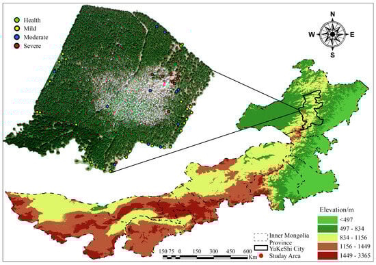
Figure 1.
Overview of the study area. The different colors in the upper left corner represent the different severity of the measured sample tree.
2.2. Ground Survey Data
Ground survey data were collected on 20 July 2024, from 51 sample trees in the test area. An A10 handheld GPS was used to record the geographic locations of the sample trees, and photometric ranging binoculars, tape measures were used to measure the tree height, diameter at breast height (DBH), east–west, north–south, and north–south crowns. In this work, the severity of larch caterpillar infestation was classified using the leaf loss rate (LLR), which is the ratio of the amount of canopy foliage loss per unit area to the amount of all foliage [27]. A total of four severity levels were classified, with 13 healthy trees (LLR: 0–5%), 16 mildly damaged trees (LLR: 6–30%), 11 moderately damaged trees (LLR: 31–60%), and 11 severely damaged trees (LLR: 61–99%). When calculating the LLR according to Equation (1), a typical standard shoot in the east, south, west, and north directions was selected at the upper (I), middle (II) and lower levels (III) of the sample tree by the tall pruning tool. The number of damaged needles and healthy needles was recorded. Finally, the average defoliation rate of all branches was used as the horizontal direction of the current sample tree to LLR. During this period, the LLR of 38 typical trees with mild, moderate, and severe stress was recorded in detail, with a total of 114 samples at the upper, middle, and lower levels of each tree, providing measured data for vertical monitoring.
2.3. Drone Data Acquisition
Hyperspectral and LiDAR data were collected on 20 July 2024, from 10:00 a.m. to 11:30 a.m. via a DJI M350 UAV (SZ DJI Technology Co., Ltd., Shenzhen, China) carrying an X20P-LIR (Hangzhou X20 Technology Co., Ltd., Hangzhou, China) sensor (shown in Figure 2). The mission was performed at an altitude of 120 m at a speed of 5 m/s, with a lateral overlap of 80% and a course overlap of 70%, with a spatial resolution of 0.49 m. The X20P-LIR sensor is a multifunctional UAV remote sensing device that integrates LiDAR, thermal infrared, RGB, panchromatic, and hyperspectral imaging for the real-time and simultaneous acquisition of multimodal remote sensing data from five sensors; the core parameters of the sensor are shown in Table 1. In this study, only hyperspectral and LiDAR data were used.
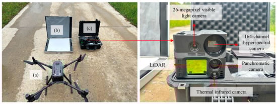
Figure 2.
UAV remote sensing data acquisition equipment: (a) DJI M350 UAV; (b) 98% reflectance-corrected whiteboard; and (c) X20P-LIR sensor.

Table 1.
Core parameters of the sensor.
2.4. Research Methods
2.4.1. Optical Indices Calculation and Preprocessing
When larch is subjected to pest stress, the appearance of the tree and the biochemical components within the needles change, and thus, its spectral reflectance also changes. The optical index provides a simple and direct reflection of vegetation conditions, and under certain conditions, it can quantitatively indicate the health of vegetation. In this work, 32 hyperspectral indices (HSIs) and multispectral indices (MSIs) were selected on the basis of the relevant literature (shown in Table A1). Among them, the MSIs were based on hyperspectral data, and the center wavelengths of five channels, namely, B1 blue (434–466 nm), B2 green (544–579 nm), B3 red (634–666 nm), B4 red-edge (714–746 nm), and B5 near-infrared (824–856 nm), were selected as the wavelengths of the multispectral bands. The center wavelength usually represents the center of the spectral response in a certain band range, which preserves the spectral properties of that band [33]. Compared with numerous band selection methods, such as particle swarm algorithms, double annealing algorithms, and differential evolution algorithms [34], the central-wavelength-based selection method not only reduces the complexity of data processing but also effectively retains the key information inherent in hyperspectral data. In particular, in fast detection and large-scale data processing scenarios, a balance between computational efficiency and accuracy can be achieved.
The above indices were calculated with ENVI (v5.6, Harris Geospatial Solutions, Broomfield, CO, USA) software, and the regions of interest of 51 sample trees were extracted via ArcGIS (v10.7, Environmental Systems Research Institute Inc., Redlands, CA, USA) software. The average value was used as the optical index of each tree and obtained using the statistics-by-region tool. On this basis, the noise level of the optical index was optimized using the S–G smoothing method [35]. S–G smoothing is suitable for spectral data processing and is able to retain peaks in the noise; thus, it is suitable for smoothing spectral reflectance data, absorption spectra, etc. This smoothing method is based on polynomial fitting, and the smoothing effect of the signal is optimized mainly by adjusting the window size (W) and polynomial order (P) [36]. The implementation steps of the method are as follows: Firstly, local polynomial fitting is carried out for each feature column, using a sliding window with sizes of 5, 7, 9, and 11 by fitting second- and third-order polynomials using least squares; Secondly, a 5-fold cross-validation is used to evaluate the smoothing performance of different combinations of parameters. For each combination, the data are split (80% for training, 20% for validation), the mean squared error (MSE) is calculated, and the combination with the smallest MSE is selected for model construction.
2.4.2. LiDAR Indices Calculation and Preprocessing
In this study, the LiDAR indices (LI) was extracted with LiDAR360 (v7.2.6, GreenValley International Inc., Berkeley, CA, USA) software after preprocessing the UAV LiDAR point cloud data with denoising, ground point classification, and normalization on the basis of ground points. The forest parameters were obtained by using the 0.1 m × 0.1 m grid calculation, including 18 LIs, including the leaf area index (LAI), canopy cover (CC), gap fraction (GF), and 15 percent percentile (PER). Here, the LAI is half of the surface area of all leaves per unit surface area, which is one of the most basic covariates characterizing the vegetation canopy structure [37] (Equation (2)). CC is the vertical projection of the stand canopy as a percentage of the forest floor area, which is an important factor in forest surveys, and an important factor reflecting the structure of the forest and the environment [38]. In (Equation (3)), GF mainly refers to the death of the old-growth trees in a forest community or the death of dominant tree species in the mature stage due to chance factors, thus creating gaps in the forest canopy [39] (Equation (4)). PER is the height at which X% of the points within each statistical cell are located within a given computational cell by sorting all normalized LiDAR point clouds within it by elevation. This includes 99%, 95%, 90%, 80%, 75%, 70%, 60%, 50%, 40%, 30%, 25%, 20%, 10%, 5%, and 1%. S–G smoothing with different combinations of parameters is similarly performed on the computed LIs to ensure the accuracy of the feature data.
2.4.3. Sensitive Feature Selection Method
The most critical step before building a model is to extract sensitive features, otherwise using too many variables will increase the computational time and complexity of the model, and affect the model results, thus not producing the best accuracy [40]. Sensitive features were screened via recursive feature elimination (RFE) on the basis of the optimal parameter combination identified through S–G smoothing. The model was iteratively trained, and the features that contributed the least to the model prediction were removed in each iteration, while most explanatory and sensitive features were retained. The algorithm was implemented via MATLAB (v2022b, MathWorks Inc., Natick, MA, USA) software. First, it trains a Bagged Regression Ensembles model on all initial features and calculates the weight or importance of each feature based on the model. Then, the model was iteratively reconstructed by eliminating the least important features in each iteration, and the process was repeated until the specified number of features was reached. Specifically, at each iteration, features with low importance were excluded, and this “recursive elimination” resulted in a set of retained features with the strongest explanatory power for model predictions. In this work, 10%, 20%, 30%, 40%, 50%, 60%, 70%, 80%, 90%, and 100% of the number of features are specified to calculate the Root Mean Squared Error (RMSE), and the changes of the RMSE are compared and observed, and the remaining features with the minimum error are selected [41]. This method can aid in identifying the optimal subset of features and maintaining good prediction performance with as few features as possible. For HSI and MSI, the RFE algorithm is used to extract the sensitive optical features, which are the estimation feature data in the horizontal direction. The sensitive features of layer I, layer II, and layer III were extracted for the LI, respectively, to provide the best sensitive features for vertical estimation.
2.4.4. Regression Model Construction
To estimate the LLR due to stress caused by larch caterpillars, sensitive optical features were identified, and with the help of the MATLAB 2022B software platform, random forest regression (RFR) and convolutional neural network regression (CNNR) were applied to build analysis models.
RFR is a nonparametric method based on the idea of integrated learning; it maximizes the accuracy and robustness of the corresponding model by combining the prediction results from multiple decision trees [42,43]. The core idea of RFR is to construct a set of independent decision tree models through out-of-bag sampling (bootstrap sampling) and stochastic feature selection, and average or vote on their predictions to obtain the final regression results [44].
CNNR is a deep learning method with a basic structure encompassing an input layer, a convolutional layer, an activation function, a pooling layer, and a fully connected layer. The convolutional layer extracts local features with sliding convolution kernels, the activation function (usually ReLU) introduces nonlinearity, and the pooling layer reduces the size of the feature map and improves computational efficiency. The advantages of CNNR are the ability to efficiently capture local patterns, the ability to share parameters that reduce model complexity, and the ability to maintain invariance to input translations for enhanced robustness [45].
2.4.5. The LLR Estimation Results Are Fused with the LiDAR Point Cloud
In this study, we fused the LLR values of sample trees estimated by remote sensing with LiDAR point cloud data with the Python (v3.8.5, Python Software Foundation, https://www.python.org/, accessed on 15 March 2025) platform to realize the three-dimensional visualization and analysis of sample trees under stress by insects. First, the pixel-level defoliation rate of the sample trees was estimated on the basis of sensitive optical and LiDAR features. Each corresponding sample tree was identified in the LiDAR point cloud dataset, and the estimation result was subjected to coordinate projection to ensure that it was aligned with the LiDAR point cloud data and to ensure that both datasets were in the same spatial reference system. Second, the geometric center of each pixel was calculated with the Geopandas library to construct the highest point cloud within the fast query range of the KD-tree, and the corresponding LLR was fused with that point. Finally, the Open3D library was used to visualize the point cloud data and tree structure in 3D. In this step, the spatial resolution of the forest tree damage result was effectively enhanced so that different severities of damage were clearly presented spatially. This method provides an efficient and accurate analysis solution for forest health monitoring.
2.4.6. Evaluation of Model Accuracy
In this work, to evaluate the performance of the regression model, the 51 sample trees in the horizontal direction and the 114 sample sizes in the vertical direction were divided into sets of 70% (36 and 80 trees) for training and 30% (15 and 34 trees) for validation. The coefficient of determination (R2) and root-mean-square error (RMSE) were used as the basic indices for the evaluation of the training model (, ) and the validation model (, ). The closer the value of the coefficient of determination is to 1, the better the model fit and the higher the estimation accuracy. Similarly, the closer the root-mean-square error is to 0, the smaller the model prediction error is and the higher the estimation accuracy. To evaluate the accuracy and stability of the models, the average value of the coefficient of determination () and the average value of the root-mean-square error () for the training and validation sets were assessed; the closer the value of is to 1 and the closer the value of is to 0, the higher the accuracy of a model is. The relative error of the coefficient of determination () and the relative error of the root-mean-square error () were used as the stability indices; the closer the two indices are to 0, the higher the model stability is. Model accuracy and stability are commonly used to characterize model performance. The model performance index (MPI) was calculated using the above metrics. The MPI ranges from 0–1, and the closer its value is to 1, the better the model performance is [46]. The formulas for the above model-performance-evaluation-related indices are shown in Table 2.
Table 2.
Calculation formula for evaluation indicators.
Where , , of MPI are the weights of the four indicators, which are determined by the analytic hierarchy process (AHP) [47,48,49]. It is realized by the judgment matrix structure, weight calculation, consistency test (CR), and other steps. According to the calculation results, the weights are = 0.33, = 0.17, = 0.33, and = 0.17, respectively, and CR = 0 proves that the matrix is consistent.
3. Results
3.1. Smoothing and Extraction of Sensitive Indices
3.1.1. S–G Smoothing Results for Different Combinations of Parameters
S–G smoothing with different combinations of window sizes (W) and polynomial orders (P) was performed for the 64 computed optical indices and 18 LiDAR indices, and the results are shown in Figure 3. As shown in Figure 3a,b, for both the HSI and MSI, the best MSEs are achieved with the W11P3 combination, where the training MSE is 0.0130 and the validation MSE is 0.0058 for the HSI and the training MSE is 0.0108 and the validation MSE is 0.0069 for the MSI. This combination not only effectively reduces noise, but also retains critical information needed for accurate modeling, providing a robust foundation for subsequent data analysis and modeling. W11P3 is fitted with a cubic polynomial based on 11 data points within the window for each fit. As shown in Figure 3a,b, as the window size increases, the MSE on the same polynomial order increases and then decreases, reaching a window size of 11. At this point, the smoothing effect is significantly improved, and the MSE is minimized, showing better data fitting ability. The LI, on the other hand, shows the opposite trend, and the optimal combination is W5P2, with MSE = 0.0285 for the training set and MSE = 0.0318 for the validation set. In contrast to the continuity of the optical features, the LiDAR features are discrete in nature; hence, owing to the characteristics of the data, the results vary for different feature types.
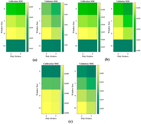
Figure 3.
Heat map of S–G smoothing results for different combinations of windows and polynomial orders for optical indices and LiDAR indices: (a) HSI; (b) MSI; and (c) LI.
3.1.2. Results of RFE-Based Sensitive Indices Extraction
For the S–G smoothed data with the W11P3 combination of optical features, the RFE algorithm was applied to calculate the RMSE for 10–100% of the features. As shown in Figure 4a, for the HSI, the optimal RMSE (0.1780) is reached when the number of features is 13 (40%), and the features are ARI, CARI, CIGREEN, EVI, GI, LCI, MCARI, NDVI, NGRDI, NPCI, NVI, PBI, and PRI. For MSI, the optimal RMSE (0.1752) is reached when the number of features is 16 (50%), and the features are ARI, CI, CIGREEN, CIREG, DVI, DVI*, DVIREG, EVIREG, GDVI, GNDVI, GOSAVI, GSAVI, INRE, INT*, LCI, and NDGI. It can be seen that multispectral data have more complex requirements for indices selection and require more comprehensive indices to achieve optimal results. In contrast, the rich information of hyperspectral data allows efficient modeling with fewer indices. For the LI, features sensitive to different vertical levels were extracted with the RFE algorithm, which is based on S–G smoothing and the W5P2 combination. As shown in Figure 4b, the lowest RMSE of 0.2696 is reached at layer I when the number of features is two. The selected features are PER 80 and PER 90. For layer II, the lowest RMSE of 0.2739 is reached when the number of features is nine. The selected features are LAI, PER1, PER 5, PER 10, PER 20, PER 25, PER 40, PER 50, and PER 60. For layer III, the lowest RMSE of 0.2768 is achieved when the number of features is 11, and the selected features are CC, PER 1, PER 10, PER 20, PER 25, PER 30, PER 40, PER 50, PER 60, PER 70, and PER 75. Horizontal and vertical LLR estimation models of forests were constructed on the basis of these sensitive HSI, MSI, and LI characteristics.
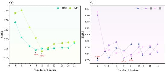
Figure 4.
Results of extracting sensitive features based on RFE algorithm: (a) HSI, MSI; and (b) LI. The arrows represent the minimum RMSE.
3.2. Model Results for LLR Estimation in the Horizontal Orientation
To compare the LLR estimation accuracy achieved with optical features at different levels of larch caterpillar pests, random forest regression (RFRHSI, RFRMSI) and convolutional neural network regression (CNNRHSI, CNNRMSI) models were applied. The models were constructed using 13 HSIs and 16 MSIs extracted via the RFE algorithm, and the regression accuracy results are shown in Figure 5 and Figure 6.
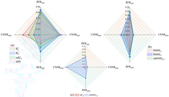
Figure 5.
Radar diagram of the accuracy and error of the LLR estimation model. (a) R2 for training and validation sets and MPI; (b) RMSE for training and validation sets; (c) The relative error of R2 and RMSE.
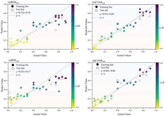
Figure 6.
Scatterplot results of the regression model: (a) RFRHSI; (b) CNNRHSI; (c) RFRMSI; and (d) CNNRMSI.
(1) The MPI of the HSI-based models exceeded 0.9, with CNNRHSI (MPI = 0.9383) outperforming RFRHSI (MPI = 0.9052). The validation results show that the values of CNNRHSI and RFRHSI are 0.9491 and 0.9314, respectively, indicating that the models are highly accurate. As shown in Figure 5a, all four evaluation metrics for the CNNRHSI model are clustered between 0.92 and 0.94, close to the edge of the radar plot. As shown in Figure 5c, the training set, validation set, and average RMSE of the CNNRHSI model are all close to the center of the radar plot, and the relative error of the model in Figure 5b is likewise close to the center of the radar plot, approaching 0, indicating that the model is stable. The four evaluation metrics for the RFRHSI in Figure 5a are scattered between 0.90 and 0.96. Although the R2 of both the RFRHSI training and validation sets reached above 0.9 with the highest prediction accuracy, the RMSEV reached 0.1756, which indicates that overfitting may occur on some of the data at the time of prediction, which reduces the MPI. The lowest LLR of the measured sample trees is 0.02, and the highest is 0.91. As shown in scatter plots in Figure 6a,b, the highest predicted value of the RFRHSI is 0.76, which is an underestimation of the LLR, whereas the lowest value of 0.1 is an overestimation, and the line of mode fit deviates slightly from the 1:1 line. The CNNRHSI model, on the other hand, yields a maximum predictive value of 0.89 and a minimum predictive value of 0.01, which are close to the true values and indicate a good fit. The comparison of the MPI accuracies of the two models constructed on the basis of the HSI results reveals that CNNRHSI > RFRHSI.
(2) The RFRMSI in the two models constructed based on MSI showed a slightly higher MPI (RFRMSI: 0.8817, CNNRMSI: 0.8712). Figure 5a shows that the of RFRMSI is greater than 0.9, whereas the of CNNRMSI is greater than 0.9, and the values are similar. Figure 5c shows that the RMSE distribution of CNNRMSI is between 0.08 and 0.12 and that of RFRMSI is between 0.14 and 0.18. Although the error is large compared with that of the CNNR, the of the CNNRMSI exceeds 0.3 and is severely off-center in the radar plot, as shown in Figure 5b. As illustrated by the scatter plots in Figure 6c,d, the RFRMSI model also suffers from underestimation of the LLR, with the highest value reaching only 0.69. Although the CNNRMSI model is well fitted, the large RMSE leads to a decrease in the MPI. The result of the comparison of the MPI accuracies of the two models constructed on the basis of MSIs is as follows: RFRMSI > CNNRMSI.
In summary, the comparison of the MPI accuracies of the four regression models reveals that CNNRHSI > RFRHSI> RFRMSI > CNNRMSI, which indicates that the accuracy of the HSI model is greater than that of the MSI model. Hundreds of consecutive spectral bands of hyperspectral data are able to capture the changes in the defoliation rate in different wavelength ranges in detail. The multispectral data, on the other hand, is based on five bands used to calculate indices, capturing relatively limited detail information and poorly characterizing different defoliation rates, resulting in comparatively poorer regression performance. Therefore, the CNNR model combined with the sensitive HSIs and different vertical layers of sensitive LIs was used to estimate the LLR in the vertical layers of the canopy with different severities of pest damage. Overall, the vertical distribution of the LLR was determined at the scale of single trees.
3.3. Model Results for LLR Estimation in the Vertical Direction
3.3.1. Results of Vertical LLR Estimation and Modeling
The CNNRHSI model is based on a horizontally oriented optimal MPI combined with LIs sensitive to different vertical layers constructed was constructed to estimate the LLR of the upper (I.), middle (II.) and lower (III.) layers of sample trees of different severity (mild, moderate and severe). A radar chart of the accuracy evaluation results is shown in Figure 7. As shown in Figure 7a, layer I has the largest area, and the accuracy indices are better than the layer II and layer III. Notably, the MPI accuracy reaches 0.8956 and the reaches a maximum of 0.9588, indicating that the model captures the data characteristics well. Moreover, as shown in Figure 7b, all the errors are smaller than the remaining two layers, distributed between 0.0 and 0.1. However, is slightly greater in this case, close to 0.3, which is within the acceptable range. Layer II has the next largest area, with four accuracy metrics scattered below 0.90 and an MPI accuracy of 0.8424. This model also exhibits the best accuracy for the training set, as indicated by the coefficient of determination of 0.8804. The model for this layer is the same as that for layer I, exhibiting slightly higher errors for , ranging between 0.3 and 0.4, with all other error metrics plotted near the center of the radar diagram. Layer III has the smallest area and performs low on all four accuracy metrics, with MPI accuracy reaching 0.8346 and exhibiting the lowest accuracy between 0.70 and 0.75. This suggests that the model, while capturing the characteristics of the data well ( above 0.85) is poorly accurate in terms of prediction. As the errors in Figure 7b show, is small for layer III compared with those for layers I and II, but is larger. The final pixel-level estimation in the vertical direction of the sample trees was obtained on the basis of this three-level model and fused with the LiDAR point cloud to obtain three-dimensional stereo estimation results. The results provide an intuitive reflection of the LLR of the larch trees under stress due to larch caterpillar infestation.
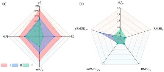
Figure 7.
Radar diagram of the accuracy and error of layer I (red), layer II (blue), and layer III (green). (a) R2 for training and validation sets and MPI; (b) RMSE for training and validation set and relative error of R2 and RMSE.
3.3.2. The 3D Visualization of LLR Estimates at Different Canopy Levels in the Vertical Direction
To assess in detail the vertically oriented distribution of the LLR for trees with mild, moderate, and severe damage due to pests, LLR estimates were obtained at the pixel level for the I, II, and III parts of the canopy on the basis of the CNNRHSI+LI model. The 3D visualization results for the single-plant-scale sample trees were combined with the LiDAR point cloud data, as shown in Figure 8. The figure shows only the results of 3D visualization for a typical sample tree in the test area and the average LLR values for all point clouds at each height level for the corresponding sample trees. Box plots of the estimation results for all sample trees in the test area are also shown.
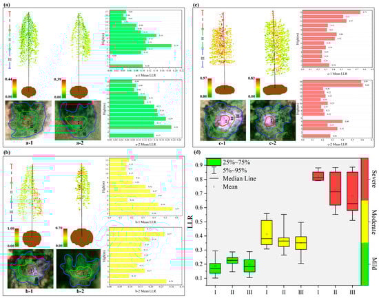
Figure 8.
Three-dimensional visualization results of vertical LLR for sample trees of different severity. (a) Three-dimensional visualization results of remote sensing images and estimation results fused with point clouds for typical mildly damaged sample trees (a-1,a-2); (b) typical moderately damaged sample trees; (c) typical severely damaged sample trees, as well as the average LLRs of all point clouds corresponding to each meter height of the corresponding sample trees (b-1,b-2); and (d) estimation results of the leaf loss rate at different levels of the vertical for all sample trees (c-1,c-2).
Figure 8a shows the results of the three-layer LLR estimation for the two mildly damaged sample trees, where the estimation of sample tree a-1 ranges from 0.00 to 0.44. Additionally, layers II and III for this sample tree are associated with moderate to low LLR values. The histogram corresponding to a-1 shows that the LLR could not be estimated at the 2–3 m position because of the lack of a point cloud, and the average LLR at the 4 m position was 0.00, which indicated extremely healthy. The LLR tended to decrease and then increase, followed by a decrease with increasing height, with the highest average LLR of 0.19 occurring at 7 m. This finding indicates that the sample trees were gradually damaged starting at the layer II position. The a-2 sample tree as a whole is associated with LLR values corresponding to moderate damage, with a range of 0.00–0.39. Additionally, the point cloud data for the lower and middle layers of this sample tree are sparse. As shown in the corresponding histogram a-2, the lack of point clouds at 2 m resulted in a failure to effectively estimate the LLR, and as the tree height increased, the LLR tended to increase but then decreased, with the highest LLR of 0.21 at 3 m. Overall, the sample tree was stressed by larch caterpillar infestation from layer III upward.
Figure 8b shows the three-level LLR estimation results for two moderately damaged sample trees, where the estimation range for sample tree b-1 is between 0 and 1. This sample tree has a white color in the right half of the remotely sensed image because of severe needle shedding due to the damage by insect pests. The 3D visualization results indicate that the right half of the right part of layer I of this sample tree lacks point cloud data, indicating that the needles and dead bark have fallen off. Conversely, the right halves of layers II and III are associated with high yellow–red LLR values due to missing leaves, and the left halves of the trees have intact needles and yellow–green LLR values. As shown in the corresponding histograms, the LLR increased, then decreased, and then increased again, followed by a decrease with height. The highest mean LR value of 0.57 was reached at 2 m, indicating that this sample tree was most victimized at the layer II and III positions. The b-2 sample tree is in a stand with a small crown, with overall yellow–green LLR values and the point cloud immediately adjacent to the trunk portion of the tree displaying reddish high LLR values, with estimates ranging from 0.00 to 0.70. As shown in the corresponding histograms, the highest mean LLR value of 0.28 was reached at 1 m, with a decreasing trend followed by an increasing LLR with height and then a decrease at the highest position.
Figure 8c shows the three-layer LLR estimation results for two severely damaged sample trees, where the estimation range of sample tree c-1 is between 0.00 and 0.97. The needles of this sample tree at the layer I position are almost shed, and only the trunk portion remains, whereas the point clouds at both the layer II and III positions display high yellow–red LLR values. As shown in the corresponding histograms, the mean LLR value increases gradually with height until the top 13 m of the tree, reaching a maximum value of 0.75. Sample tree c-2 was also similarly severely damaged at the stratum I position with complete loss of needles. However, the point cloud at the layer II and III positions had lower LLR compared to sample tree c-1, showing green–yellow–red LLR values, with estimates ranging from 0.00 to 0.83. As shown in the corresponding histograms, missing point cloud data at 2 and 6 m result in failed estimation. The mean LLR value increases and then decreases with height, reaching the highest mean value (0.60) at the top tree position.
As shown in Figure 8d, the LLR tends to increase with increasing severity. The mean value of the LLR of the number of lightly damaged samples tended to increase and then decrease at different levels vertically. The estimation range of the sample trees was concentrated between 0.1 and 0.3, where 25–75% of the point cloud LLRs in stratum I were concentrated between 0.14 and 0.20, indicating limited damage. Layer II, with a 25–75% point cloud LLR ranging from 0.20–0.25, was more concentrated and had a higher LLR than layer I. The LLR of layer III was the highest. For layer III, 25–75% of the point cloud LLRs were concentrated between 0.15–0.25. The mean LLR values of the moderately damaged sample trees tended to decrease at different levels vertically. The estimated range of LLR for the sample trees was between 0.20 and 0.55, with the largest box in stratum I. A total of 25–75% of the LLRs were distributed between 0.30 and 0.50 and were dispersed. For layer II, 25–75% of the LLRs were distributed from 0.3–0.4 and were highly concentrated. For layer III, 25–75% of the LLRs were distributed between 0.3–0.4 and were more dispersed than those for layer II. The mean LLR values of the heavily damaged sample trees showed a decreasing trend at different levels vertically. The LLR estimates for the sample trees ranged from 0.50–0.90, with 25–75% of the LLRs in layer I distributed in the range of 0.80–0.90, and these values were relatively concentrated. Moreover, 25–75% of the LLRs in layer II were distributed between 0.60–0.85 and relatively dispersed. For layer III, 25–75% of the LLRs were distributed between 0.55–0.85 and were more dispersed than those for layer II.
In summary, the sample trees with different levels of damage presented vertical differences in LLR. Among them, all the mildly damaged sample trees gradually started to be damaged in the middle and lower (II and III) layers, whereas the moderately damaged sample trees did not display a clear damage pattern, and the severely damaged sample trees all showed a pattern of serious damage in the top (I) layer. The results provide an important reference for forestry departments and forest-health monitoring.
4. Discussion
4.1. Performance of Multi-Source Remote Sensing Features for LLR Estimation
In this study, in order to estimate the LLR of forest trees under larch caterpillar infestation, multisource features combined with machine learning algorithms were extracted to construct an accurate estimation model in both horizontal and vertical directions, which provides a powerful research method for pest control. In this study, S–G smoothing is introduced to reduce the noise of the data to provide a more accurate data source for the extraction of sensitive features. Savitzky and Golay invented S–G smoothing, which removes noise while preserving the signal form and broadband [35]. Existing studies have focused on S–G smoothing preprocessing of spectral data, including UAV spectral noise removal [50,51,52], and satellite remote sensing time series [53], in order to enhance the accuracy of vegetation index calculation. However, the innovation of this study is the S–G smoothing of optical features and LiDAR features with different combinations of windows (5, 7, 9, 11) and polynomial orders (2, 3), and the optimal combination pattern is explored. Compared with traditional methods, this approach can better fit the characteristics of UAV remote sensing data, effectively reduce the influence of environmental noise and improve the stability of features. It also compensates for the application of S–G smoothing in the optimization of multisource remote sensing features from UAVs, thus enhancing the reliability of the model estimation performance and providing higher quality data support for applications such as forest health monitoring. In a study applying S–G smoothing to UAV hyperspectral data, an overall accuracy of 93.47% was obtained for the classification of rice leaf blight [54]. In contrast, this study extracted sensitive features to construct the LLR estimation model after preprocessing remote sensing features based on S–G smoothing with different parameter combinations, and obtained an accuracy of 93.83%, which indicates that parameter tuning can enhance the data quality in order to improve the estimation model accuracy. The extraction of sensitive features can effectively improve the prediction accuracy of the model and also optimize the computational efficiency and enhance the generalization ability of the model [55]. The recursive feature elimination (RFE) algorithm chosen in this paper is a commonly used feature selection method, which removes unimportant features recursively and evaluates the performance of different feature subsets to ultimately determine the optimal feature combination [56]. The histogram of the feature importance scores of the 13 HSIs and 16 MSIs extracted according to this algorithm is shown in Figure 9. The difference in importance scores of HSI and MSI features in the model can be seen in Figure 9a. For the HSIs, features such as the NDVI, ARI and MCARI exhibit high importance scores, especially the NDVI, with a score of more than 0.7. This index is a common vegetation index used in remote sensing; it is calculated from the reflectance of the near-infrared (800 nm) and red light (670 nm) bands and displays strong sensitivity to the health status of trees, biomass, etc. [57,58]. The ARI and MCARI are highly sensitive to changes in leaf carotenoids and chlorophyll [59], which can be used to distinguish vegetation with different health levels; these features play a key role in model performance. In addition, other common HSIs, such as the NPCI, PRI, and LCI, also have high scores, reflecting their advantages when using hyperspectral data, as they effectively reflect information on vegetation status and health conditions [60]. However, some features, such as the NVI, PBI, and NGRDI, had low importance scores, indicating that these features contributed comparatively less to the estimation of LLR. In contrast, the performance of the MSIs was slightly different, with high importance scores for GOSAVI and GNDVI, especially for GOSAVI, with a value close to 0.6, indicating its importance in multispectral data processing. Other common vegetation indices, such as the LCI, NDGI, and CIGREEN, also enhance modeling performance in cases with multispectral features. Overall, however, the importance scores for MSIs were generally lower than those for HSIs, which may be related to the number of bands considered. The hundreds of bands of hyperspectral data provide more fine-scale information, and the corresponding indices dominate the feature importance scores, whereas the features of multispectral data, although also of some importance, display lower importance scores overall. This suggests that hyperspectral data have a greater advantage over multispectral data in tasks that require fine-scale differentiation between different vegetation conditions or health states. As shown in Figure 9b, PER90 in stratum I had the highest importance score, exceeding 0.8, indicating that the height variable at the 90th percentile position of the stand was consistent with the layer I characteristics of the stand [61]. PER80, on the other hand, had a lower importance score, but an MPI accuracy of 0.8956 was obtained for the LLR estimation model constructed for layer I, suggesting that the use of two feature types enhanced the estimation ability of the model through synergistic effects. The differences in the importance scores of most features in layer II are small, with PER1 having the highest contribution. PER5 and PER10 had the smallest importance scores, which may have affected the accuracy of the model. The importance scores of features other than PER10 in layer III were small compared with those in layers I and II, whereas PER10 had the second-highest importance score among all features in the three layers and highly contributed to the estimates of the model. In summary, the drawback of this paper is that features with low importance scores are not eliminated, which may lead to the introduction of redundant information or noise into the model, thus affecting the training efficiency and estimation accuracy of the model. Although the model has some predictive ability at different vertical levels, the unoptimized feature set may make the model complex and increase the risk of overfitting. In future research, features of low importance should be eliminated to improve the generalization ability of the model, reduce the number of computations, and further optimize model performance.
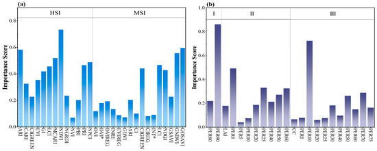
Figure 9.
Histograms of importance scores for LLR-sensitive features: (a) HSI and MSI; and (b) LI sensitive to different levels of the vertical.
4.2. Application of Multidimensional Estimation of LLR to Forest Management
Compared with the traditional time-consuming and labor-intensive methods of obtaining forest LLR, the remote sensing approach with UAV-based hyperspectral and LiDAR data collection shortens the cycle of data acquisition, improves the data accuracy, and provides a technical basis for the large-scale, nondestructive inversion of forest biochemical parameters. In this study, a model with optimal accuracy in the horizontal direction combined with LI sensitive to three levels was used to realize LLR estimation in the vertical direction. Then, the results were fused with LiDAR point cloud data to achieve 3D visualization. Numerous articles have been published on multisource data fusion for the inversion of forest parameters, among which the DSM-based fusion method proposed by Xin Shen and other researchers from Nanjing Forestry University in 2020 is the most advanced. The team accomplished the fusion of hyperspectral and LiDAR data via three steps: generating a gridded LiDAR point cloud, extracting the highest-quality LiDAR point cloud data, and matching the hyperspectral pixels to those points. A regression model was then implemented to predict forest biochemical traits at three vertical canopy levels, and an R2 of 0.85–0.91 was obtained [22]. Recently, the method has also been applied to multispectral and LiDAR data fusion and hyperspectral, thermal infrared, and LiDAR data fusion to investigate the 3D photosynthetic shape of winter wheat and the vertical profile of plant shape under pine wood nematode stress [18,23]. Inspired by this work, we demonstrated the vertical spatial distribution of the LLR of sample trees under stress due to larch caterpillar infestation by fusing the pixel-level estimated LLR with LiDAR point cloud data via Python. It is found that the estimated MPI reaches 0.93 in the horizontal direction and between 0.83 and 0.89 in the vertical direction, and this accuracy is close to that of Xin Shen, Qinan Lin et al. [18,22]. The LLR multidimensional estimation method proposed in this paper achieves high accuracy and innovatively realizes 3D visualization, but still has several limitations at the operational level. For example, it requires high-precision, ground-survey data acquisition, especially the canopy top data are still difficult to obtain; and the method relies on high-resolution LiDAR data for 3D visualization, thus reaching at most the application on the stand scale. The application of this method to the stand scale in subsequent studies can further explore the overall response under pest stress. In forest management applications, the method has demonstrated important value for accurate pest management and disaster assessment. Its three-dimensional visualization capability at the single-tree scale can not only provide decision support for targeted application and selective harvesting, but also through the comprehensive analysis of the vertical spatial distribution of different forest stands. It can reveal the impact of pests on the growth and health of the entire forest stand, and accurately identify the most significant areas of pest infestation, thus providing data support for the precise application of control measures. This multidimensional assessment breaks through the limitations of traditional two-dimensional monitoring, enabling managers to formulate differentiated management strategies based on the actual damage of each layer of the canopy, and significantly improving the pertinence and effectiveness of control measures.
5. Conclusions
In this study, the optical and lidar features sensitive to LLR were extracted by combining UAV multisource remote sensing data with S–G smoothing and RFE algorithms. Random Forest Regression (RFR) and Convolutional Neural Network Regression (CNNR) models were constructed to estimate the horizontal and vertical LLR under larch caterpillar pest stress. The study concluded as follows:
- (1)
- The S–G smoothing of different parameter combinations shows completely opposite conclusions on the optical features (W11P3) and the LiDAR features (W5P2), which is due to the characteristics of the data.
- (2)
- Combined with the RFE algorithm, 13 HSIs and 16 MSIs were extracted horizontally, and the analysis found that the HSI had higher importance scores than MSI, especially NDVI and ARI. Six LIs were extracted from layer I, nine from layer II, and eleven from layer III at different vertical levels, and the same analysis found that PER90, PER1, and PER10 had the highest importance scores respectively.
- (3)
- The MPI ranking of the horizontal model constructed based on sensitive optical features is CNNRHSI > RFRHSI > RFRMSI > CNNRMSI, where CNNRHSI achieves the best accuracy (MPI = 0.9383).
- (4)
- The combination of CNNRHSI and sensitive LI constructs a vertically different level LLR estimation model. It was found that the accuracy of the CNNRHSI+LI model reached more than 0.8 (layer I: MPI = 0.8956, layer II: MPI = 0.8424, layer III: MPI = 0.8346), and the accuracy was reliable. Finally, the estimation results of the single tree scale were fused with the LiDAR point cloud to realize the three-dimensional visualization of LLR. The results showed that the mildly damaged sample trees were gradually damaged from the II and III layers; the severely damaged sample trees were severely damaged on the I layer; and the moderately damaged sample trees did not show obvious patterns.
The method proposed in this study not only addresses the shortcomings of the traditional two-dimensional model but also provides intuitive results for the index of tree leaf loss rate after insect infestation grazing, and improves the accurate estimation ability of LLR.
Author Contributions
H.-Y.S., X.H. and L.L.: Writing—original draft, Visualization, Validation, Software, Methodology, Conceptualization. Y.B.: Writing—review & editing, Supervision, Funding acquisition, Project administration. D.Z. and J.Z.: Supervision, Resources, Funding acquisition. G.B. and S.T.: Supervision, Project administration, Methodology, Funding acquisition, Conceptualization. D.G., D.A. and D.E.: Writing—review & editing, Supervision, Methodology, Conceptualization. M.A.: Validation. All authors have read and agreed to the published version of the manuscript.
Funding
This study was supported by the National Natural Science Foundation of China (42361057), the Young Scientific and Technological Talents in High Schools (NJYT22030), the Ministry of Education Industry-University Cooperative Education Project (202102204002).
Data Availability Statement
Data are contained within the article.
Conflicts of Interest
The authors declare no conflicts of interest.
Appendix A
Table A1.
Optical index and its calculation formula.
Table A1.
Optical index and its calculation formula.
| HSI | Formula | MSI | Formula |
|---|---|---|---|
| NPCI [62] | (670 − 460)/(670 + 460) | GNDVI [33] | (B5 − B2)/(B5 + B2) |
| SR [63] | 750/550 | DVI [63] | B5 − B3 |
| MRENDVI [64] | (752 − 702)/(752 + 702) | RVI [63] | B5/B3 |
| PSRI [64] | (680 − 500)/750 | GOSAVI [65] | (B5 − B2)/(B5 + B2 + 0.16) |
| PBI [66] | 810/560 | OSAVIREG [65] | (B5 − B4)/(B5 + B4 + 0.16) |
| PRI [66] | (531 − 570)/(531 + 570) | AR [67] | 1/B2 − 1/B4 |
| LCI [68] | (850 − 710)/(850 + 710) | GDVI [69] | B5 − B2 |
| RARS [70] | 760/500 | TVI [71] | 0.5(120(B5 − B2) − 200(B3 − B2)) |
| CSRI [70] | (760/500) | CIREG [71] | B5/B4 − 1 |
| NDVI [72] | (800 − 670)/(800 + 670) | CIGREEN [71] | B5/B2 − 1 |
| GI [73] | 554/677 | CI [71] | B5/B2 − 1 |
| REP [74] | 700 + 40 × (((670 + 780)/2) − 700)/(740 − 700) | RCI [75] | B5/B3 − 1 |
| NVI [76] | (777 − 747)/673 | NDVI [77] | (B5 − B3)/(B5 + B3) |
| ARI [78] | (1/550) − (1/700) | SAVI [79] | 1.5(B5 − B3)/(B5 + B3 + 0.5) |
| CARI [80] | (700 − 670) − 0.2 × (700 − 550) | GSAVI [81] | 1.5(B5 − B2)/(B5 + B2 + 0.5) |
| EVI [82] | 2.5 × ((830 − 660)/(1 + 830 + 6 × 660 − 7.5∗465)) | OSAV [83] | (B5 − B3)/(B5 + B3 + 0.16) |
| MCARI [84] | ((700 − 670) − 0.2∗(700 − 550))∗(700/670) | EVI [85] | 2.5(B5 − B3)/(B5 + 6 × B3 − 7.5 × B1 + 1) |
| NGRDI [86] | (550 − 660)/(550 + 660) | NDGI [87] | (B2 − B3)/(B2 + B3) |
| RCI1 [88] | 750/710 | GMSR [89] | (B5/B2 − 1)/(B5/B2 + 1)0.5 |
| RCI2 [90] | 850/710 | DVIREG [91] | B5 − B4 |
| RECI [92] | (760/725) − 1 | EVIREG [91] | 2.5(B5 − B4)/(B5 + 6 × B4 − 7.5 × B1 + 1) |
| CIGREEN [92] | (1/750–1/550)/550 | RVIREG [93] | B5/B4 |
| TCARI [94] | 3 × ((700 − 670) − 0.2 × (700 − 550) × (700 − 670)) | MSRREG [95] | (B5/B4 − 1)/(B5/B4 + 1)0.5 |
| CIREG [94] | ((1/750) − (1/700))/700 | NDVI* [96] | (B4 − B3)/(B4 + B3) |
| CRI1 [65] | (1/508) − (1/549) | DVI* [97] | (B4 − B3) |
| CRI2 [65] | (1/508) − (1/702) | INT* [93] | (B4 + B3)/2 |
| RECRI [98] | ((1/510) − (1/710)) × 790 | NDSI* [99] | (B3 − B4)/(B3 + B4) |
| GRVI [100] | (872/559) | RVI* [101] | B4/B3 |
| MTCI [102] | (742 − 702)/(702 + 661) | LCI [103] | (B5 − B2)/(B5 + B2) |
| MTCI2 [104] | (742 − 712)/(712 + 661) | InRE [105] | 100 × (B5 − B3) |
| NDRSR [106] | (872 − 712)/(872 + 712) | INT2* [93] | (B2 + B3 + B4)/2 |
| RSR [107] | 872/712 | MSR [108] | (B5/B3 − 1)/(B5/B3)0.5 + 1) |
References
- Wang, Y.-H.; Zhou, G.-S.; Jing, Y.-L.; Yang, Z.-Y. Estimating Biomass and NPP of Larix Forests using forest inventory data. Chin. J. Plant Ecol. 2001, 25, 420–425. [Google Scholar]
- Li, W.; Shu, L.; Wang, M.; Li, W.; Yuan, S.; Si, L.; Zhao, F.; Song, J.; Wang, Y. Temporal and Spatial Distribution and Dynamic Characteristics of Lightning Fires in the Daxing’anling Mountains from 1980 to 2021. Sci. Silvae Sin. 2023, 59, 22–31. [Google Scholar]
- Cong, J.X.; Wang, G.P.; Han, D.X.; Gao, C. Organic matter sources in permafrost peatlands changed by high-intensity fire during the last 150years in the northern Great Khingan Mountains, China. Palaeogeogr. Palaeoclimatol. Palaeoecol. 2023, 631, 111821. [Google Scholar] [CrossRef]
- Zhang, J.; Hao, L. Occurence of Dendrolimus superans in Daxing’anling of Inner Mongolia and Its Management. For. Sci. Technol. 2002, 27, 26–28. [Google Scholar] [CrossRef]
- Zhu, H.; Lin, C.; Liu, G.; Wang, D.; Qin, S.; Li, A.; Xu, J.-L.; He, Y. Intelligent agriculture: Deep learning in UAV-based remote sensing imagery for crop diseases and pests detection. Front. Plant Sci. 2024, 15, 1435016. [Google Scholar] [CrossRef] [PubMed]
- Liu, F.; Qu, C.; Xiao, N.; Chen, G.; Tang, W.; Wang, Y. A Study on Spectral Characteristics and Chlorophyll Content in Rice. Acta Laser Biol. Sin. 2017, 26, 326–333. [Google Scholar] [CrossRef]
- Liu, L.; Peng, Z.; Zhang, B.; Han, Y.; Wei, Z.; Han, N. Monitoring of Summer Corn Canopy SPAD Values Based on Hyperspectrum. J. Soil Water Conserv. 2019, 33, 353–360. [Google Scholar] [CrossRef]
- Zhang, N.; Zhang, X.; Yang, G.; Zhu, C.; Huo, L.; Feng, H. Assessment of defoliation during the Dendrolimus tabulaeformis Tsai et Liu disaster outbreak using UAV-based hyperspectral images. Remote Sens. Environ. 2018, 217, 323–339. [Google Scholar] [CrossRef]
- Zhao, R.; Zhang, B.; Zhang, C.; Chen, Z.; Chang, N.; Zhou, B.; Ke, K.; Tang, F. Goji Disease and Pest Monitoring Model Based on Unmanned Aerial Vehicle Hyperspectral Images. Sensors 2024, 24, 6739. [Google Scholar] [CrossRef]
- He, R.; Li, H.; Qiao, X.; Jiang, J. Using wavelet analysis of hyperspectral remote-sensing data to estimate canopy chlorophyll content of winter wheat under stripe rust stress. Int. J. Remote Sens. 2018, 39, 4059–4076. [Google Scholar] [CrossRef]
- Liu, W.; Li, Y.; Tomasetto, F.; Yan, W.; Tan, Z.; Liu, J.; Jiang, J. Non-destructive Measurementsof Toona sinensis Chlorophylland Nitrogen Content Under Drought Stress Using Near Infrared Spectroscopy. Front. Plant Sci. 2022, 12, 809828. [Google Scholar] [CrossRef]
- Li, M.; Zhu, X.; Li, W.; Tang, X.; Yu, X.; Jiang, Y. Retrieval of Nitrogen Content in Apple Canopy Based on Unmanned Aerial Vehicle Hyperspectral Images Using a Modified Correlation Coefficient Method. Sustainability 2022, 14, 1992. [Google Scholar] [CrossRef]
- Johari, S.N.A.M.; Khairunniza-Bejo, S.; Shariff, A.R.M.; Husin, N.A.; Masri, M.M.M.; Kamarudin, N. Detection of Bagworm Infestation Area in Oil Palm Plantation Based on UAV Remote Sensing Using Machine Learning Approach. Agriculture 2023, 13, 1886. [Google Scholar] [CrossRef]
- Yin, D.; Wang, L.; Lu, Y.; Shi, C. Mangrove tree height growth monitoring from multi-temporal UAV-LiDAR. Remote Sens. Environ. 2024, 303, 114002. [Google Scholar] [CrossRef]
- Wang, L.; Zhang, R.; Zhang, L.; Yi, T.; Zhang, D.; Zhu, A. Research on Individual Tree Canopy Segmentation of Camellia oleifera Based on a UAV-LiDAR System. Agriculture 2024, 14, 364. [Google Scholar] [CrossRef]
- Brede, B.; Calders, K.; Lau, A.; Raumonen, P.; Bartholomeus, H.M.; Herold, M.; Kooistra, L. Non-destructive tree volume estimation through quantitative structure modelling: Comparing UAV laser scanning with terrestrial LIDAR. Remote Sens. Environ. 2019, 233, 111355. [Google Scholar] [CrossRef]
- He-Ya, S.; Huang, X.; Zhou, D.; Zhang, J.; Bao, G.; Tong, S.; Bao, Y.; Ganbat, D.; Tsagaantsooj, N.; Altanchimeg, D.; et al. Identification of Larch Caterpillar Infestation Severity Based on Unmanned Aerial Vehicle Multispectral and LiDAR Features. Forests 2024, 15, 191. [Google Scholar] [CrossRef]
- Lin, Q.; Huang, H.; Wang, J.; Chen, L.; Du, H.; Zhou, G. Early detection of pine shoot beetle attack using vertical profile of plant traits through UAV-based hyperspectral, thermal, and LiDAR data fusion. Int. J. Appl. Earth Obs. Geoinf. 2023, 125, 103549. [Google Scholar] [CrossRef]
- Hakala, T.; Suomalainen, J.; Kaasalainen, S.; Chen, Y. Full waveform hyperspectral LiDAR for terrestrial laser scanning. Opt. Express 2012, 20, 7119–7127. [Google Scholar] [CrossRef]
- Bi, K.; Xiao, S.; Gao, S.; Zhang, C.; Huang, N.; Niu, Z. Estimating vertical chlorophyll concentrations in maize in different health states using hyperspectral LiDAR. IEEE Trans. Geosci. Remote Sens. 2020, 58, 8125–8133. [Google Scholar] [CrossRef]
- Hao, Y.-S.; Niu, Y.-F.; Wang, L.; Bi, K.-Y. Exploring the Capability of Airborne Hyperspectral LiDAR Based on Radiative Transfer Models for Detecting the Vertical Distribution of Vegetation Biochemical Components. Spectrosc. Spectr. Anal. 2024, 44, 2083–2092. [Google Scholar] [CrossRef]
- Shen, X.; Cao, L.; Coops, N.C.; Fan, H.; Wu, X.; Liu, H.; Wang, G.; Cao, F. Quantifying vertical profiles of biochemical traits for forest plantation species using advanced remote sensing approaches. Remote Sens. Environ. 2020, 250, 112041. [Google Scholar] [CrossRef]
- Yang, T.; Yu, Y.; Yang, X.; Du, H. UAV hyperspectral combined with LiDAR to estimate chlorophyll content at the stand and individual tree scales. Chin. J. Appl. Ecol. 2023, 3, 2101–2112. [Google Scholar] [CrossRef]
- Lu, J.; Chen, J.; Li, W.; Zhou, M.; Hu, J.; Tian, W.; Li, C. Research on Classification of Pest and Disease Tree Samples Based on Hyperspectral LiDAR. Laser Optoelectron. Prog. 2021, 58, 519–525. [Google Scholar] [CrossRef]
- Wang, G.; Aierken, N.; Chai, G.; Yan, X.; Chen, L.; Jia, X.; Wang, J.; Huang, W.; Zhang, X. A novel BH3DNet method for identifying pine wilt disease in Masson pine fusing UAS hyperspectral imagery and LiDAR data. Int. J. Appl. Earth Obs. Geoinf. 2024, 134, 104177. [Google Scholar] [CrossRef]
- Huo, L. Research on Pine Tree Defoliation Estimation Using Single-scan Terrestrail Laser Scanning Data. Ph.D. Thesis, Beijing Forestry University, Beijing, China, 2019. [Google Scholar] [CrossRef]
- Huang, X.-J.; Xie, Y.-W.; Bao, Y.-H.; Bao, G.; Qing, S.; Bao, Y.-L. Estimation of Leaf Loss Rate in Larch Infested with Erannis jacobsoni Djak Based on Differential Spectral Continuous Wavelet Coefficient. Spectrosc. Spectr. Anal. 2019, 39, 2732–2738. [Google Scholar] [CrossRef]
- Huang, X.-J.; Xie, Y.-W.; Bao, Y.-H. Spectral Detection of Damaged Level Affected by Jas, s Larch Inchworm. Spectrosc. Spectr. Anal. 2018, 38, 905–911. [Google Scholar] [CrossRef]
- Yang, L.; Huang, X.; Bao, Y.; Bao, G.; Tong, S. Sudubilig. Effects of UAV flight altitude on the accuracy of monitoring Dendrolimus superans pests by remote sensing. J. Nanjing For. Univ. 2023, 47, 13–22. [Google Scholar] [CrossRef]
- Sun, G.; Huang, X.; Dashzebeg, G.; Ariunaa, M.; Bao, Y.; Bao, G.; Tong, S.; Dorjsuren, A.; Davaadorj, E. Discrimination of Larch Needle Pest Severity Based on Sentinel-2 Super-Resolution and Spectral Derivatives—A Case Study of Erannis jacobsoni Djak. Forests 2025, 16, 88. [Google Scholar] [CrossRef]
- Bai, X.-Q.; Zhang, X.-L.; Zhang, N.; Zhang, L.-S.; Ma, Y.-B. Monitoring model of dendrolimus tabulaeformis disaster using hyperspectral remote sensing technology. J. Beijing For. Univ. 2016, 38, 16–22. [Google Scholar] [CrossRef]
- Bai, X.-Q. Disaster Degree Retrieval of Dendrolimus Tabulae Based on Hyperspectral Remote Sensing Technology. Master’s Thesis, Beijing Forestry University, Beijing, China, 2017. [Google Scholar] [CrossRef]
- Gitelson, A.A.; Kaufman, Y.J.; Merzlyak, M.N. Use of a green channel in remote sensing of global vegetation from EOS-MODIS. Remote Sens. Environ. 1996, 58, 289–298. [Google Scholar] [CrossRef]
- Zelinski, M.; Mastin, A.; Castillo, V.; Yoxall, B. Optimal band selection for target detection with a LWIR multispectral imager. J. Appl. Remote Sens. 2022, 16, 026505. [Google Scholar] [CrossRef]
- Savitzky, A.; Golay, M.J. Smoothing and differentiation of data by simplified least squares procedures. Anal. Chem. 1964, 36, 1627–1639. [Google Scholar] [CrossRef]
- Fu, Y.; Yang, G.J.; Song, X.Y.; Li, Z.H.; Xu, X.G.; Feng, H.K.; Zhao, C.J. Improved estimation of winter wheat aboveground biomass using multiscale textures extracted from UAV-based digital images and hyperspectral feature analysis. Remote Sens. 2021, 13, 581. [Google Scholar] [CrossRef]
- Chen, J.M.; Black, T.A. Measuring leaf area index of plant canopies with branch architecture. Agric. For. Meteorol. 1991, 57, 1–12. [Google Scholar] [CrossRef]
- Jennings, S.B.; Brown, N.D.; Sheil, D. Assessing forest canopies and understorey illumination: Canopy closure, canopy cover and other measures. Forestry 1999, 72, 59–73. [Google Scholar] [CrossRef]
- Richardson, J.J.; Moskal, L.M.; Kim, S.H. Modeling approaches to estimate effective leaf area index form aerial discrete-return LIDAR. Agric. For. Meteorol. 2009, 149, 1152–1160. [Google Scholar] [CrossRef]
- Varin, M.; Chalghaf, B.; Joanisse, G. Object-Based Approach Using Very High Spatial Resolution 16-Band WorldView-3 and LiDAR Data for Tree Species Classification in a Broadleaf Forest in Quebec, Canada. Remote Sens. 2020, 12, 3092. [Google Scholar] [CrossRef]
- Chen, X.; Sun, Y.; Guo, S.; Duan, Y.; Tang, A.; Ye, Z.; Zhang, H. Urban Tree Species Classification by UAV Visible Light Imagery and OBIA-RF Model. J. Northeast For. Univ. 2024, 52, 48–59. [Google Scholar] [CrossRef]
- Yu, K.; Yao, X.; Qiu, Q.; Liu, J. Landslide Spatial Prediction Based on Random Forest Model. Trans. Chin. Soc. Agric. Mach. 2016, 47, 338–345. [Google Scholar] [CrossRef]
- Ahmadm, W.; Reynolds, J.; Rezgui, Y. Predictive modelling for solar thermal energy systems: A comparison of supportvector regression, random forest, extra trees and regression trees. J. Clean. Prod. 2018, 203, 810–821. [Google Scholar] [CrossRef]
- Breiman, L. Random forests. Mach. Learn. 2001, 45, 5–32. [Google Scholar] [CrossRef]
- Cacciari, I.; Ranfagni, A. Hands-On Fundamentals of 1D Convolutional Neural Networks—A Tutorial for Beginner Users. Appl. Sci. 2024, 14, 8500. [Google Scholar] [CrossRef]
- Huang, X.-J. Remote Sensing Identification and Monitoring of Larch Needle Pests Based on Ground Hyperspectral Data. Ph.D. Thesis, Lanzhou University, Gansu, China, 2019. [Google Scholar] [CrossRef]
- Saaty, T.L. Decision making with the analytic hierarchy process. Int. J. Serv. Sci. 2008, 1, 83–98. [Google Scholar] [CrossRef]
- Saaty, R.W. The analytic hierarchy process-what it is and how it is used. Math. Model. 1987, 9, 161–176. [Google Scholar] [CrossRef]
- Vaidya, O.S.; Kumar, S. Analytic hierarchy process: An overview of applications. Eur. J. Oper. Res. 2006, 169, 1–29. [Google Scholar] [CrossRef]
- Yin, C.; Wang, Z.; Lv, X.; Qin, S.; Ma, L.; Zhang, Z.; Tang, Q. Reducing soil and leaf shadow interference in UAV imagery for cotton nitrogen monitoring. Front. Plant Sci. 2024, 15, 1380306. [Google Scholar] [CrossRef]
- Wang, D.; Sun, X.; Zhang, Y.; Xia, H.; Lu, M.; Zhou, L. Spectral Characteristics of Water Stress in Chili Pepper Leaves. Trans. Chin. Soc. Agric. Mach. 2024, 55, 336–344. [Google Scholar] [CrossRef]
- Gao, A.; Qiao, F.; Zhu, W.; Zhong, X.; Deng, Y. Prediction of moisture content of hummus peach based on multi-burr hyperspectral data. Food Mach. 2023, 39, 123–129. [Google Scholar] [CrossRef]
- Cai, Z.; Jönsson, P.; Jin, H.; Eklundh, L. Performance of Smoothing Methods for Reconstructing NDVI Time-Series and Estimating Vegetation Phenology from MODIS Data. Remote Sens. 2017, 9, 1271. [Google Scholar] [CrossRef]
- Liu, Z.-Y.; Feng, S.; Zhao, D.-X.; Li, J.-P.; Guan, Q.; Xu, T.-Y. Research on Spectral Feature Extraction and Detection Method of Rice Leaf Blast by UAV Hyperspectral Remote Sensing. Spectrosc. Spectr. Anal. 2024, 44, 1457–1463. [Google Scholar] [CrossRef]
- Guo, J.; Huang, X.; Zhou, D.; Zhang, J.; Bao, G.; Tong, S.; Bao, Y.; Ganbat, D.; Altanchimeg, D.; Enkhnasan, D.; et al. Estimation of the water content of needles under stress by Erannis jacobsoni Djak. via Sentinel-2 satellite remote sensing. Front. Plant Sci. 2025, 16, 1540604. [Google Scholar] [CrossRef] [PubMed]
- Wu, C.; Liang, J.; Wang, W.; Li, C. Random Forest Algorithm Based on Recursive Feature Elimination. Stat. Decis. 2017, 21, 60–63. [Google Scholar] [CrossRef]
- Wei, W.; Jing, X.-L.; Ge, X.-Y.; Sun, L.; Lu, Z. Long-Short NDVI Time Series Method for Detecting Local Mutation Characteristics of Vegetation. Adm. Tech. Environ. Monit. 2023, 35, 28–34. [Google Scholar] [CrossRef]
- Mo, K.; Chen, Q.; Chen, C.; Zhang, J.; Wang, L.; Bao, Z. Spatiotemporal variation of correlation between vegetation cover and precipitation in an arid mountain-oasis river basin in northwest China. J. Hydrol. 2019, 574, 138–147. [Google Scholar] [CrossRef]
- Sytar, O.; Bruckova, K.; Kovar, M.; Zivcak, M.; Hemmerich, L.; Brestic, M. Nondestructive detection and biochemical quantification of buckwheat leaves using visible (VIS) and near–infrared (NIR) hyperspectral reflectance imaging. J. Cent. Eur. Agric. 2017, 18, 864–878. [Google Scholar] [CrossRef]
- Wu, C.-Y.; Niu, Z. Review of retrieval light use efficiency using photochemical reflectance index (PRI). Chin. J. Plant Ecol. 2008, 32, 734–740. [Google Scholar] [CrossRef]
- Park, T. Potential Lidar Height, Intensity, and Ratio Parameters for Plot Dominant Species Discrimination and Volume Estimation. Remote Sens. 2020, 12, 3266. [Google Scholar] [CrossRef]
- Patrick, A.; Pelham, S.; Culbreath, A.; Holbrook, C.C.; De Godoy, I.J.; Li, C. High throughput phenotyping of tomato spot wilt disease in peanuts using unmanned aerial systems and multispectral imaging. IEEE Instrum. Meas. Mag. 2017, 20, 4–12. [Google Scholar] [CrossRef]
- Jordan, C.F. Derivation of Leaf-Area Index from Quality of Light on the Forest Floor. Ecology 1969, 50, 663–666. [Google Scholar] [CrossRef]
- Sims, D.A.; Gamon, J.A. Relationships between leaf pigment content and spectral reflectance across a wide range of species, leaf structures and developmental stages. Remote Sens. Environ. 2002, 81, 337–354. [Google Scholar] [CrossRef]
- Gitelson, A.A.; Kaufman, Y.J.; Stark, R.; Rundquist, D. Novel algorithms for remote estimation of vegetation fraction. Remote Sens. Environ. 2002, 80, 76–87. [Google Scholar] [CrossRef]
- Gamon, J.; Serrano, L.; Surfus, J. The photochemical reflectance index: An optical indicator of photosynthetic radiation use efficiency across species, functional types, and nutrient levels. Oecologia 1997, 112, 492–501. [Google Scholar] [CrossRef] [PubMed]
- Gitelson, A.A.; Merzlyak, M.N. Remote estimation of chlorophyll content in higher plant leaves. Int. J. Remote Sens. 1997, 18, 2691–2697. [Google Scholar] [CrossRef]
- Datt, B. A new reflectance index for remote sensing of chlorophyll content in higher plants: Tests using Eucalyptus leaves. J. Plant Physiol. 1999, 154, 30–36. [Google Scholar] [CrossRef]
- Main, R.; Cho, M.A.; Mathieu, R.; O’Kennedy, M.M.; Ramoelo, A.; Koch, S. An investigation into robust spectral indices for leaf chlorophyll estimation. Isprs J. Photogramm. Remote Sens. 2011, 66, 751–761. [Google Scholar] [CrossRef]
- Chappelle, E.W.; Kim, M.S.; Iii, M.M. Ratio analysis of reflectance spectra (RARS): An algorithm for the remote estimation of the concentrations of chlorophyll A, chlorophyll B, and carotenoids in soybean leaves. Remote Sens. Environ. 1992, 39, 239–247. [Google Scholar] [CrossRef]
- Gitelson, A.A.; Viña, A.; Arkebauer, T.J.; Rundquist, D.C.; Keydan, G.; Leavitt, B. Remote estimation of leaf area index and green leaf biomass in maize canopies. Geophys. Res. Lett. 2003, 30, 1248. [Google Scholar] [CrossRef]
- Tucker, C.J. Red and photographic infrared linear combinations for monitoring vegetation. Remote Sens. Environ. 1979, 8, 127–150. [Google Scholar] [CrossRef]
- le Maire, G.; François, C.; Dufrêne, E. Towards universal broad leaf chlorophyll indices using PROSPECT simulated database and hyperspectral reflectance measurements. Remote Sens. Environ. 2004, 89, 1–28. [Google Scholar] [CrossRef]
- Clevers, J.G.P.W. Imaging Spectrometry in Agriculture—Plant Vitality And Yield Indicators. In Imaging Spectrometry—A Tool for Environmental Observations; Eurocourses: Remote Sensing, Volume 4; Hill, J., Mégier, J., Eds.; Springer: Dordrecht, The Netherlands, 1994. [Google Scholar] [CrossRef]
- Soukhovolsky, V.G.; Krasnoperova, P.A.; Palnikova, E.N.; Sviderskaya, I.V.; Tarasova, O.V. Differences in the Dynamics of Radial Tree Increment in the Pine Looper Outbreak Area and in Undamaged Stands and Assessment of the Risk of Pests’ Attack. Contemp. Probl. Ecol. 2019, 12, 753–759. [Google Scholar] [CrossRef]
- Gupta, R.K.; Vijayan, D.; Prasad, T.S. New hyperspectral vegetation characterization parameters. Adv. Space Res. 2001, 28, 201–206. [Google Scholar] [CrossRef]
- Tucker, C.J.; Elgin, J.H.; Mcmurtrey, J.E.; Fan, C. Monitoring corn and soybean crop development with hand-held radiometer spectral data. Remote Sens. Environ. 1979, 8, 237–248. [Google Scholar] [CrossRef]
- Gitelson, A.A.; Merzlyak, M.N.; Chivkunova, O.B. Optical properties and nondestructive estimation of anthocyanin content in plant leaves. Photochem. Photobiol. 2001, 74, 38–45. [Google Scholar] [CrossRef] [PubMed]
- Huete, A.R. A Soil-Adjusted Vegetation Index (Savi). Remote Sens. Environ. 1988, 25, 295–309. [Google Scholar] [CrossRef]
- Kim, M.S. The Use of Narrow Spectral Bands for Improving Remote Sensing Estimation of Fractionally Absorbed Photosynthetically Active Radiation (fAPAR). Master’s Thesis, University of Maryland, College Park, MD, USA, 1994. [Google Scholar] [CrossRef]
- Yang, M.D.; Tseng, H.H.; Hsu, Y.C.; Tsai, H.P. Semantic Segmentation Using Deep Learning with Vegetation Indices for Rice Lodging Identification in Multi-date UAV Visible Images. Remote Sens. 2020, 12, 633. [Google Scholar] [CrossRef]
- Huete, A.; Didan, K.; Miura, T.; Rodriguez, E.P.; Gao, X.; Ferreira, L.G. Overview of the radiometric and biophysical performance of the MODIS vegetation indices. Remote Sens. Environ. 2002, 83, 195–213. [Google Scholar] [CrossRef]
- Rondeaux, G.; Steven, M.D.; Baret, F. Optimized of Soil-adjusted vegetation indices. Remote Sens. Environ. 1996, 55, 95–107. [Google Scholar] [CrossRef]
- Daughtry, C.; Walthall, C.; Kim, M.; De Colstoun, E.B.; McMurtrey, J., III. Estimating corn leaf chlorophyll concentration from leaf and canopy reflectance. Remote Sens. Environ. 2000, 74, 229–239. [Google Scholar] [CrossRef]
- Jiang, Z.Y.; Huete, A.R.; Didan, K.; Miura, T. Development of a Two-Band Enhanced Vegetation Index without a Blue Band. Remote Sens. Environ. 2008, 112, 3833–3845. [Google Scholar] [CrossRef]
- Hunt, E.R.; Cavigelli, M.; Daughtry, C.S.T.; McMurtrey, J.E.; Walthall, C.L. Evaluation of digital photography from model aircraft for remote sensing of crop biomass and nitrogen status. Precis. Agric. 2005, 6, 359–378. [Google Scholar] [CrossRef]
- Mirik, M.; Ansley, R.J.; Michels, G.J.; Elliott, N.C. Spectral vegetation indices selected for quantifying Russian wheat aphid (Diuraphis noxia) feeding damage in wheat (Triticum aestivum L.). Precis. Agric. 2012, 13, 501–516. [Google Scholar] [CrossRef]
- Zarco-Tejada, P.J.; Miller, J.R.; Noland, T.L.; Mohammed, G.H.; Sampson, P.H. Scaling-up and model inversion methods with narrowband optical indices for chlorophyll content estimation in closed forest canopies with hyperspectral data. IEEE Trans. Geosci. Remote Sens. 2001, 39, 1491–1507. [Google Scholar] [CrossRef]
- Knyazikhin, Y.; Martonchik, J.V.; Myneni, R.B.; Diner, D.J.; Running, S.W. Synergistic algorithm for estimating vegetation canopy leaf area index and fraction of absorbed photosynthetically active radiation from MODIS and MISR data. J. Geophys. Res. Atmos. 1998, 103, 32257–32275. [Google Scholar] [CrossRef]
- Coops, N.C.; Stone, C.; Culvenor, D.S.; Chisholm, L.A.; Merton, R.N. Chlorophyll content in eucalypt vegetation at the leaf and canopy scales as derived from high resolution spectral data. Tree Physiol. 2003, 23, 23–31. [Google Scholar] [CrossRef] [PubMed]
- Broge, N.H.; Leblanc, E. Comparing prediction power and stability of broadband and hyperspectral vegetation indices for estimation of green leaf area index and canopy chlorophyll density. Remote Sens. Environ. 2001, 76, 156–172. [Google Scholar] [CrossRef]
- Gitelson, A.A.; Keydan, G.P.; Merzlyak, M.N. Three-band model for noninvasive estimation of chlorophyll, carotenoids, and anthocyanin contents in higher plant leaves. Geophys. Res. Lett. 2006, 33, 2–6. [Google Scholar] [CrossRef]
- Yang, N.; Cui, W.; Zhang, Z.; Zhang, J.; Chen, J.; Du, R.; Lao, C.; Zhou, Y. Soil salinity inversion at different depths using improved spectral index with UAV multispectral remote sensing. Trans. Chin. Soc. Agric. Eng. 2020, 36, 13–21. [Google Scholar] [CrossRef]
- Haboudane, D.; Miller, J.R.; Tremblay, N.; Zarco-Tejada, P.J.; Dextraze, L. Integrated narrow-band vegetation indices for prediction of crop chlorophyll content for application to precision agriculture. Remote Sens. Environ. 2002, 81, 416–426. [Google Scholar] [CrossRef]
- Chen, J.M. Evaluation of Vegetation Indices and a Modified Simple Ratio for Boreal Applications. Can. J. Remote Sens. 1996, 22, 229–242. [Google Scholar] [CrossRef]
- Gitelson, A.; Merzlyak, M.N. Quantitative estimation of chlorophyll-a using reflectance spectra: Experiments with autumn chestnut and maple leaves. J. Photochem. Photobiol. B Biol. 1994, 22, 247–252. [Google Scholar] [CrossRef]
- Richardsons, A.J.; Wiegand, A. Distinguishing vegetation from soil background information. Photogramm. Eng. Remote Sens. 1977, 43, 1541–1552. [Google Scholar]
- Jacquemoud, S.; Ustin, S.L.; Verdebout, J.; Schmuck, G.; Andreoli, G.; Hosgood, B. Estimating leaf biochemistry using the PROSPECT leaf optical properties model. Remote Sens. Environ. 1996, 56, 194–202. [Google Scholar] [CrossRef]
- Richardson, A.D.; Duigan, S.P.; Berlyn, G.P. An evaluation of noninvasive methods to estimate foliar chlorophyll content. New Phytol. 2002, 153, 185–194. [Google Scholar] [CrossRef]
- Sripada, R.P.; Heiniger, R.W.; White, J.G.; Meijer, A.D. Aerial Color Infrared Photography for Determining Early In-Season Nitrogen Requirements in Corn. Agron. J. 2006, 98, 968–977. [Google Scholar] [CrossRef]
- Major, D.J.; Baret, F.; Guyot, G. A ratio vegetation index adjusted for soil brightness. Int. J. Remote Sens. 1990, 11, 727–740. [Google Scholar] [CrossRef]
- Dash, J.; Curran, P.J. The MERIS terrestrial chlorophyll index. In Proceedings of the IEEE International Geoscience and Remote Sensing Symposium (IGARSS), Anchorage, AK, USA, 20–24 September 2004; pp. 1–257. [Google Scholar] [CrossRef]
- Haboudane, D.; Miller, J.R.; Pattey, E.; Zarco-Tejada, P.J.; Strachan, I.B. Hyperspectral vegetation indices and novel algorithms for predicting green LAI of crop canopies: Modeling and validation in the context of precision agriculture. Remote Sens. Environ. 2004, 90, 337–352. [Google Scholar] [CrossRef]
- Dash, J.; Curran, P.J. Evaluation of the meris terrestrial chlorophyll index (mtci). Adv. Space Res. 2007, 39, 100–104. [Google Scholar] [CrossRef]
- Gong, P.; Pu, R.; Biging, G.S.; Larrieu, M.R. Estimation of forest leaf area index using vegetation indices derived from Hyperion hyperspectral data. IEEE Trans. Geosci. Remote Sens. 2003, 41, 1355–1362. [Google Scholar] [CrossRef]
- Gitelson, A.A.; Vina, A.; Ciganda, V.; Rundquist, D.C.; Arkebauer, T.J. Remote estimation of canopy chlorophyll content in crops. Geophys. Res. Lett. 2005, 32, L08403. [Google Scholar] [CrossRef]
- Gitelson, A.A.; Chivkunova, O.B.; Merzlyak, M.N. Nondestructive estimation of anthocyanins and chlorophylls in anthocyanic leaves. Am. J. Bot. 2009, 96, 1861–1868. [Google Scholar] [CrossRef]
- Slater, P.N.; Jackson, R.D. Atmospheric effects on radiation reflected from soil and vegetation as measured by orbital sensors using various scanning directions. Appl. Opt. 1982, 21, 3923–3931. [Google Scholar] [CrossRef]
Disclaimer/Publisher’s Note: The statements, opinions and data contained in all publications are solely those of the individual author(s) and contributor(s) and not of MDPI and/or the editor(s). MDPI and/or the editor(s) disclaim responsibility for any injury to people or property resulting from any ideas, methods, instructions or products referred to in the content. |
© 2025 by the authors. Licensee MDPI, Basel, Switzerland. This article is an open access article distributed under the terms and conditions of the Creative Commons Attribution (CC BY) license (https://creativecommons.org/licenses/by/4.0/).