1. Introduction
In recent years, unmanned aerial vehicles (UAVs) have widely been adopted in various real-life scenarios to execute various missions successfully with path planning being the key factor behind their success and the safe flight [
1,
2,
3,
4,
5]. For autonomous flights, path planning is indispensable for navigating the UAV to various targets to accomplish various missions without human intervention. Path-planning algorithms can be categorized into two main streams: classical or conventional and intelligent algorithms. Classical algorithms include Dijkstra, A-star, dynamic A, rapidly-exploring random trees (RRTs), probabilistic roadmaps (PRMs), potential fields, and genetic algorithms [
6,
7,
8], while the intelligent algorithms are based on reinforcement learning and neural networks predictors [
9,
10,
11].
Conventional path-planning algorithms for UAVs struggle to address the suboptimality in 3D robot environments and face the issue of local optima. To solve such problems, researchers have recently adopted algorithms from reinforcement learning with deep learning, rendering improved and dynamic path-planning methods for mobile robots and UAVs [
9,
12,
13]. In a recent study [
14], the authors have proposed a Q-learning-based RL approach for UAV path planning in both static and dynamic environments. By formulating the obstacle assessment model and path-planning task as a Markov decision process (MDP), they define a structured state space, action space, and reward function to optimize trajectory generation. To enhance exploration efficiency, the authors integrate a heuristic-guided ε-greedy policy, which strategically biases action selection toward promising regions of the state space. This modification significantly improves both learning convergence and policy effectiveness compared to random exploration. Empirical results demonstrate that their method outperforms conventional path-planning techniques, including A*, RRT, and standard DQN, in terms of computational efficiency and path optimality. A related study [
15] also employs a Q-learning-based RL approach for UAV path planning in environments with both static and dynamic obstacles. The method introduces a distance-based prioritization policy, leveraging the Euclidean distance between the start and goal points to guide action selection. While the study accounts for dynamic obstacles, its policy learning is limited to single-goal scenarios. Similarly, obstacle avoidance and path planning for a UAV have been done using the Q-learning algorithm in [
16]. Authors in [
17] address the single-goal path-planning problem for UAVs by proposing a deep reinforcement learning (DRL) framework that integrates deep neural networks (DNNs) with an actor-critic architecture. This approach enables the UAV agent to learn an optimal action policy for autonomous trajectory generation. The actor-critic-based DRL framework enhances the agent’s capability to handle high-dimensional state spaces and continuous action domains, leading to more efficient behavior optimization in complex environments. The same has been discussed in a survey study on actor-critic-based reinforcement learning in [
18]. In [
19], the authors have used DNNs and Q-learning to realize a deep Q-network to learn a policy for UAV path planning. This study incorporates artificial potential fields with the traditional DQN to present an improved variant of the algorithm. Similarly, authors in [
20,
21,
22,
23] have discussed DRL-based methods for path planning of various kinds of UAVs. Policy gradient (PG) is another DRL algorithm that is used commonly for various sequential decision-making problems. In [
24], authors have presented a two-stage RL framework for multi-UAV path planning using the PG algorithm. Similarly, the study in [
25] discusses a deep deterministic policy gradient (DDPG)-based control framework for learning and autonomous decision-making capability for UAVs. The reviewed literature indicates that reinforcement learning methods are increasingly being adopted by researchers to address path-planning challenges for aerial agents.
Traditional Q-learning is a widely adopted reinforcement learning algorithm due to its inherent advantages of algorithmic simplicity and its ability to adapt effectively to dynamic environments [
26,
27]. However, it faces numerous shortcomings and related problems resulting in suboptimal path planning in high-dimensional robot environments.
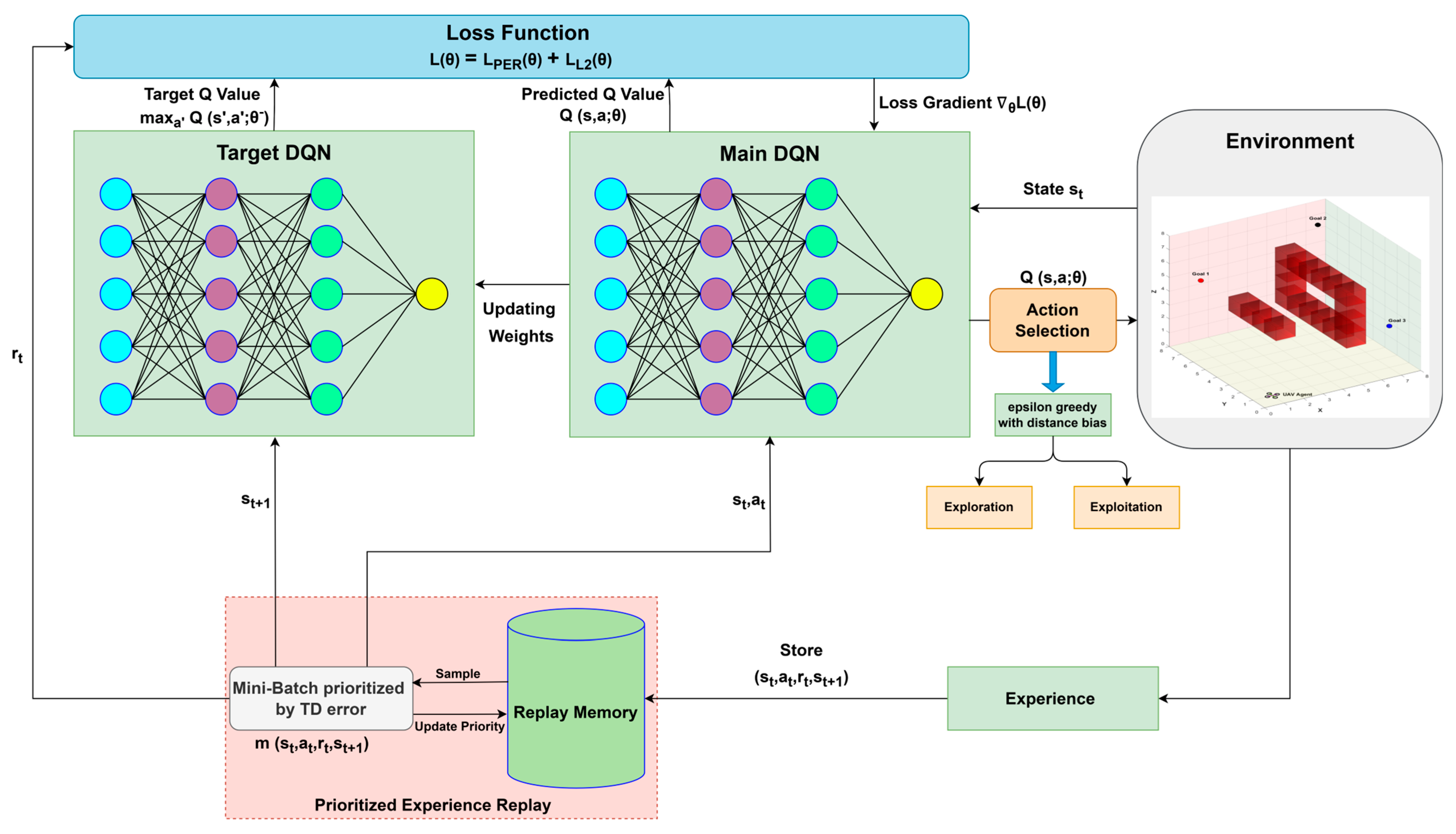
Figure 1 illustrates the fundamental RL-based UAV path-planning framework. The agent interacts with the UAV environment by selecting actions based on its current policy, while receiving feedback in the form of rewards and updated states. This interaction loop enables the agent to iteratively improve its policy for optimal trajectory planning in complex 3D environments. The key challenges in existing approaches include inefficient action selection, simplistic reward structures, and slow convergence rates [
28]. These limitations often result in the generation of random and suboptimal UAV paths in 3D obstacle-cluttered environments [
29]. The baseline DQN relies solely on current experiences to update the Q-values, which frequently leads to slow learning and poor policy performance due to data inefficiency and the presence of highly correlated training samples. The DQN with experience replay (DQN-ER) addresses this issue by storing past transitions and sampling them randomly, thereby reducing temporal correlation and stabilizing the training process [
30]. This technique enhances policy robustness, particularly during the early exploration phase. However, uniform sampling in experience replay treats all transitions equally, which diminishes the influence of rare but valuable experiences. DQN with reward shaping (DQN-RS) seeks to overcome this by designing structured reward signals that guide the agent’s behavior, even when the goal state is not immediately achieved [
31]. Despite its potential, improper reward shaping can lead to unintended learning outcomes. Overall, a persistent limitation across DQN and its variants is their tendency to produce random action selections, which, even when occasionally optimal, often result in suboptimal UAV trajectories.
To solve these problems, this paper proposes an improved deep Q-learning algorithm leveraging the use of deep neural networks. The proposed deep Q-network (DQN-Proposed) algorithm combines multiple enhancements to address different limitations of traditional DQN. The improved action selection by efficiently breaking the ties between equally valued Q-actions renders an optimal path and ultimately the optimal UAV trajectory with minimum length. This modified tie-breaking mechanism ensures consistent behavior when Q-values are similar and prevents random oscillations in policy due to numerical ties in action selection. This mechanism is not deterministic in early training stages due to the stochastic nature of exploration and thus does not cause the agent to prematurely converge to suboptimal policies. Importantly, the agent still relies on Q-value estimates to guide exploration and learning. The tie-breaking rule does not override the learned policy but only aids in disambiguating equally valued actions. In practice, this reduces policy jitters and leads to smoother convergence, without introducing additional risk of being trapped in local optima.
To improve the convergence and stability, we have incorporated the prioritized experience reply and L2-regularization. In traditional experience replay, transitions (state, action, reward, next state) are stored and sampled uniformly during training. Experiences with higher TD errors (i.e., surprising or poorly learned ones) are more likely to be revisited and learned from. Based on temporal difference error, PER introduces a priority score for each transition and focuses on the most informative transitions. Hard-to-learn examples are revisited more frequently, which accelerates the overall learning. This also allows the agent to learn from fewer, high-impact experiences rather than wasting time on well-predicted and low-impact ones. Moreover, rare and high-reward experiences (e.g., reaching a goal) are prioritized, which helps the agent to rediscover these valuable states and improve learning. For better stability, PER allows the use of high-error samples that correct the Q-network more effectively which ultimately prevent it from getting stuck in suboptimal policies.
Path planning in three-dimensional (3D) environments involves many state-action pairs that cause poor generalization. In the proposed Q-learning approach, we have incorporated L2-regularization to prevent the network from memorizing specific paths and to generalize to unseen obstacles and routes. This also encourages smaller weights that lead to more stable and smoother Q-values to reduce the erratic action selections (e.g., sudden direction changes) and encourages smoother UAV flight paths. In complex 3D grids, overfitting to early exploration data can trap the UAV in suboptimal paths. L2 keeps the model flexible enough to adapt to better policies later. Together, these techniques create a more stable, sample-efficient, and goal-directed learning framework that outperforms all other DQN variants in both training and test environments.
The key contributions of this paper are as follows:
- 1.
An improved Q-learning algorithm based on deep neural networks is proposed for autonomous UAV navigation in complex 3D obstacle-cluttered environments.
- 2.
A dynamic action-value adjustment mechanism is introduced to enhance action selection, reduce randomness, and promote the generation of more optimal UAV trajectories.
- 3.
Prioritized experience replay is employed to accelerate convergence by sampling transitions with high temporal difference error thus avoiding the inefficiencies of uniform sampling.
- 4.
The replay buffer is designed to emphasize high-reward experiences (e.g., goal-reaching states), which allows the agent to revisit and learn more effectively from valuable states.
- 5.
L2-regularization is integrated into the learning process to constrain weight magnitudes that lead to smoother Q-value updates, reduced erratic behavior, and more stable UAV flight paths.
The remainder of this paper is as follows:
Section 2 provides background information related to UAV model and reinforcement learning.
Section 3 presents problem formulation and the proposed Q-learning approach to solve the navigation problem of a UAV in a 3D environment.
Section 4 elaborates the experimental setting and results followed by a detailed discussion on the results obtained. Finally,
Section 5 concludes this study.
2. Background
This section presents a concise yet comprehensive overview of the theoretical foundations essential for understanding the proposed UAV navigation framework. It covers key concepts in quadrotor dynamics, the principles of deep reinforcement learning, and the Q-learning algorithm with emphasis on their relevance to autonomous path planning in complex 3D environments.
2.1. Mathematical Model of a Quadrotor UAV
This section presents a set of well-established equations of a quadrotor model from [
32]. This model is used for trajectory generation in
Section 4 and acts as an agent in an MDP environment.
The translational states of the quadrotor UAV can be written as follows:
where
is the total thrust vector produced by the four rotors and controls the vertical motion,
is the mass of the UAV,
, and
,
, and
are the second order derivatives of (acceleration terms) of translation states
of quadrotor UAV.
The rotational states of the quadrotor model can be written as follows:
where
, and
are torques around the roll (
), pitch (
), and yaw axes (
), respectively, which control the UAV’s orientation and rotational motion. The terms
and
denote the inertia tensor,
is the rotor inertia, and
is the relative speed of cross-coupled rotor pairs,
are the acceleration terms, and
are the velocity terms of rotational states
of the quadrotor, respectively.
2.2. Deep Reinforcement Learning
Reinforcement learning enables an agent to interact with an environment to maximize cumulative rewards. Deep reinforcement learning combines RL with deep learning to handle complex decision-making tasks in high-dimensional environments. Unlike classical RL, which uses Q-tables, DRL employs deep neural networks to approximate Q-values and policies directly from raw inputs. This allows agents to generalize better and learn more effectively in large state and action spaces. Core components of DRL include the agent, which selects actions based on a policy; the environment, which responds with rewards and state updates; and value functions, e.g., and , which estimate expected long-term rewards. DRL has driven substantial progress in diverse domains such as robotics, autonomous systems, and strategic game playing.
Q-learning is a fundamental model-free reinforcement learning algorithm that allows an agent to learn how to make optimal decisions in an environment by estimating the Q-function. The Q-function represents the expected cumulative reward for taking a specific action in a given state and then following the optimal policy thereafter. Unlike other methods, Q-learning does not require a prior model of the environment which confers that it does not need to know how the environment works in advance. This makes it highly versatile and applicable to a wide range of problems, from game playing to autonomous decision-making in robotics. In the Q-learning algorithm, the Q-table stores the estimated Q-values for each state-action pair. Initially, these values are set to zero or small random numbers. The agent interacts with the environment by observing the current state, selecting an action (often using an -greedy strategy to balance exploration and exploitation), and receiving a reward while transitioning to a new state. The Q-value for the chosen state-action pair is then updated using the Bellman equation, which incorporates the immediate reward and the discounted maximum Q-value of the next state. This process repeats over many episodes and gradually refines the Q-values until they converge to their optimal values. Finally, this enables the agent to learn the best actions for each state.
The Q-function is updated using the Bellman equation [
33], which expresses the relationship between the current Q-value and the future Q-values. The Q-learning update rule can be described as follows:
where
is the learning rate,
is the immediate reward,
is the discount factor (how much future rewards are valued),
is the maximum Q-value for the next state
.
Q-learning formulation can be described using the Q-value, which represents the expected cumulative reward starting from state , taking action , and following the optimal policy thereafter.
The optimal policy can be extracted as follows:
To balance the exploration, actions can be selected using the following
-greedy strategy:
where
balances exploration and exploitation.
3. Proposed DQN Framework
3.1. Problem Formulation
Path-planning problem for an aerial agent in a 3D environment can be formulated as a finite episodic MDP assuming that the terms and are finite and , , and .
For 3D path planning, an arbitrary finite navigation space can be defined as follows:
where
and
are states and
defines the total number of MDP states.
The navigation environment is modeled as a discrete 3D grid indexed by row , column , and altitude , where each cell represents a unique spatial state. The action space comprises six deterministic motions corresponding to unit transitions along the primary axes: forward , backward , left , right , upward , and downward . These actions enable the UAV agent to explore the environment in all three spatial dimensions which form the basis for state transitions within the Markov decision process framework.
The corresponding finite action space is
where
are the index terms of
and
, respectively.
The reward function is formulated as follows:
where
represent the terminal or the goal state of the navigation task, and
denote the obstacles in the occupancy grid map. The reward values in Equation (12) were chosen to provide clear guidance to the agent during learning: a strong positive reward (+100) for reaching the goal to reinforce success, a strong penalty (−100) for hitting obstacles to discourage collisions, and a small negative reward (−1) for all other states to encourage shorter, more efficient paths.
The simulator generates an occupancy grid map using environmental image data as input. Various kinds of grids, such as squares, rectangles, triangles, and trapezoids can be used to discretize the environment in the occupancy map. In our designed simulator, square boxes are used to discretize the environment and to generate the grid map. The size of the grid cell determines the accuracy, safety, and computational time of the algorithm and therefore this parameter needs to be chosen carefully depending on the real-time dimensions of the environment.
3.2. Proposed DQN Approach
For a given state
and all possible actions
, we can write the Q-value function for the main DQN as follows:
The term represents the output of deep neural network for input state , which is encoded into a feature vector. The output is a vector of Q-values for all possible actions given a state . The term also represents the neural network function approximation for Q-value learning.
We can formulate
as follows:
where
is input layer of DNN.
For hidden layers
, we can write
where
, and
for each layer
and
is activation function which is ReLU in our case.
The output layer of DNN is defined as follows:
where
represents the learnable network parameters and output
is a vector
of size
and
, while
represents the number of possible actions.
The DNN is trained to minimize the mean squared error (MSE) between the predicted Q-values and the target Q-values .
The loss function can be written as follows:
We can define the target Q-value function
as follows:
where
represents the parameters of target DQN which is a copy of the main DQN that is updated periodically
. The term
represents prioritized experience replay buffer which stores past experiences
.
To minimize the loss function
, the parameters
of the DQN are updated using the gradient descent algorithm and the gradient update rule is as follows:
where
is learning rate and
is the gradient of the loss with respect to
.
The policy
is derived using an
-greedy strategy:
The variable decay rate can be set as follows:
where
is initial exploration rate,
is minimum exploration rate, and
is decay rate that controls how fast
drops.
The goal is to learn the optimal Q-function
that maximizes the cumulative discounted reward:
To implement the prioritized experience replay, each experience
in the replay buffer
is assigned a priority
which determines its likelihood of being sampled. Priority is typically based on the temporal-difference error
.
The temporal-difference error
is
where
denotes the TD error for the
-th experience, and
is small positive constant to ensure all experiences have a non-zero chance of being sampled.
The probability
of sampling experience
is proportional to its priority as follows:
where
is a hyperparameter with range
and controls the tradeoff between greedy prioritization (
) and uniform sampling (
).
normalizes the probability.
To correct the bias introduced by prioritized sampling, each sampled experience is weighted by the following importance sampling weight [
33]:
where
is the size of the replay buffer,
is a hyperparameter that controls the degree of bias correction with range
.
From (17) and (26), we can now modify the loss function to account for prioritization as follows:
To prevent overfitting, we penalize the large weights in DNN using the weight decay approach also known as L-2 regularization as follows:
where
is the regularization coefficient that controls the penalty strength,
shows the total number of DNN layers, and
is squared L2-norm of all weight vectors of DNN.
The modified loss function with L2-regularization becomes
Let
, for gradient descent the weight update now includes the regularization gradient as follows:
The added term encourages weights to stay smaller and prevents the overfitting of DNN.
Due to limited action space, there may exist more than one optimal policy, each generating similar Manhattan cost. However, during trajectory generation these policies may generate different path lengths. In order to render an optimal policy that ultimately reduces the path length, we have proposed a modified Q-value selection (action- selection) mechanism as given subsequently.
It is quite possible to have multiple actions that have near-identical Q-values during the greedy policy phase. Let
denote the action space,
represent the Q-value for action
in state
, and
be a small positive threshold for tie-breaking. The set of near-optimal actions
is defined as follows:
From these candidates
, valid actions
are filtered to exclude those leading to obstacles or out-of-bounds states:
The final action
is selected by minimizing the Euclidean distance to the
:
where
is Euclidean distance.
This rule integrates with the ε-greedy policy
as follows:
The exploration rate follows the Equation (21) and decays over time to balance the exploration and exploitation.
For transitions where tie-breaking occurred, the TD target becomes
where
uses the same tie-breaking logic during target computation.
Similarly, the tie-breaking-based policy affects the priority calculation of PER as follows:
Based on these theoretical developments, we propose a modified DQN approach in Algorithm 1. This algorithm has been used to conduct different experimental tests in our designed RL simulator.
Figure 2 shows the schematic of the proposed DQN approach that has been adopted in this work.
| Algorithm 1 Proposed DQN with modified tie-breaking based policy, PER, and L2 regularization |
| 1: | Input: |
| 2: | Environmental states actions |
| 3: | Reward function :
|
| 4: | Hyperparameters: , , , . |
| 5: | Output: Trained Q-network |
| 6: | procedure Initialize |
| 7: | Main Q-network , target network with |
| 8: | Prioritized replay buffer with capacity |
| 9: | |
| 10: | end procedure |
| 11: | for episode to do |
| 12: | Reset environment to |
| 13: | while is not terminal do |
| 14: |
Action Selection (Policy): |
| 15: | if then |
| 16: | random action from |
| 17: |
else |
| 18: |
|
| 19: |
|
| 20: |
|
| 21: | if then |
| 22: |
|
| 23: |
else |
| 24: |
|
| 25: |
end if |
| 26: |
end if |
| 27: | Execute , observe |
| 28: |
Store Transition: |
| 29: |
|
| 30: |
|
| 31: | Store |
| 32: |
Sample Mini-Batch: |
| 33: | Sample K transitions with |
| 34: | Compute importance sampling weights |
| 35: |
Compute Loss with PER and L2: |
| 36: | for each transition if is non-terminal do |
| 37: |
|
| 38: |
end for |
| 39: |
|
| 40: |
Update Parameters: |
| 41: | Perform gradient descent |
| 42: | Update target network |
| 43: | for sampled transitions and update |
| 44: | Decay exploration rate |
| 45: | Set |
| 46: |
end while |
| 47: | end for |
3.3. Analysis of DQN Convergence
This section provides a formal derivation of the convergence guarantees of DQN based on classical reinforcement learning theory. The proof structure builds upon the contraction property of the Bellman operator and the Banach Fixed-Point Theorem, while incorporating assumptions relevant to function approximation and DQN-specific mechanisms such as target networks and experience replay.
Definition 1 (Bellman Operator) [33]. Let be an action-value function over states and actions . The Bellman operator is defined as follows: , where is the discount factor. Definition 2 (Banach Fixed-Point Theorem) [34]. If is a contraction mapping on a complete metric space , then has a unique fixed point such that and for any initial point , the sequence converges to Lemma 1 (Contraction Mapping). The Bellman optimality operator is a -contraction in the sup-norm and for any two Q-functions and , it satisfies the following:
Hence, is a -contraction under the supremum norm.
Assumption 1. Let be a neural network approximator. The projection operator
maps any Q-function to the closest representable
:
Assumption 2. We have bounded function approximation error if there exists such that
Theorem 1 ( is a contractor). The DQN performs approximate dynamic programming by repeatedly applying
. Under Assumptions 1 and 2, the composed operator
satisfies
where is a contraction-like constant and is approximation error. Proof of Theorem 1. By Lemma 1:
Now projecting this onto
via
and using triangular inequality,
Let
be the worst-case approximation error, then
If
is small, this resembles a contractor:
This completes the proof. □
Assumption 3 (Lipschitz Continuity) [35]. Let be two action-value functions and let denote the projection operator onto the function class representable by a neural network, then is assumed to be -Lipschitz continuous: where represents the Lipschitz constant of the projection operator .
Corollary 1 (Stable DQN Iteration). Under Assumptions 1–3, if , then is a contractor with coefficient .
Proof. Combine Theorem 1 with Assumption 3. □
Corollary 2 (Approximate Fixed-Point Convergence). If approximation error is small , then DQN converges to neighborhood of where is the desired precision constant which ensures the fixed point is within of .
Proof. From Theorem 1, the iteration is a contractor mapping with error . The result follows from Banach Fixed-Point Theory for approximate contractions.
In deep Q-networks, is approximated using a neural network Although function approximation introduces non-linearities and potential divergence, using techniques such as target networks and experience replay helps stabilize training. Recent results show that under bounded approximation error and regular updates of target network parameters, DQN can approximate a contraction mapping which leads to empirical convergence. □
3.4. UAV Trajectory Generation
The trajectory generation problem needs to meet multiple task requirements such as flight efficiency, obstacle avoidance, and dynamical feasibility to enable the development of an extensible planner [
36]. In our study, the resulting waypoint sequence from RL planner is refined into a dynamically feasible trajectory using the differential flatness property of quadrotor dynamics. This ensures that the final desired trajectory respects the UAV’s motion constraints and smoothness requirements that make it suitable for real-world execution. While our learning-based planner focuses on geometric efficiency during training, the differential flatness-based optimization acts as a post-processing layer to ensure that global feasibility and dynamic consistency are preserved. This two-stage approach allows us to prioritize simplicity and convergence speed during learning, while still achieving practical feasibility in execution.
Following the differential flatness theorem for quadrotor UAV from [
37], the selected flat outputs from the quadrotor model (1–6) are
. To ensure efficient motion and minimize control effort during UAV flight, it is essential to reduce the higher-order derivatives of position, particularly the snap, which refers to the fourth derivative of translational states
with respect to time [
38]. Minimizing snap leads to smoother trajectories and reduces the burden on actuators, thereby enhancing energy efficiency and mechanical stability. To achieve this objective, the translational trajectory
is designed to minimize snap throughout the flight duration. Consequently, the optimal desired trajectory
must satisfy specific smoothness constraints and assume the following analytical form:
where
is equal to
for minimum snap trajectory.
Now, the Euler–Lagrange equation can be solved as follows:
This yields the following condition:
The solution of (51) produces the optimal trajectory in the following form:
For selected UAV flat outputs
from (1–6), using (52), a complete trajectory can be formulated over various time slots as follows:
where
defines the degree of polynomial.
Equation (53) computes the desired optimal UAV trajectory in terms of selected flat outputs of the UAV model. This trajectory inherently satisfies the UAV’s dynamic and motion constraints and serves as the basis for generating the corresponding control commands. The derivation of these commands is usually handled as a classical control problem. The controller that we have implemented in our simulation environment can be found in [
39].
4. Experiments and Results
We have conducted various experiments in our simulator designed exclusively for RL-based UAV navigation. The simulator is custom-developed in MATLAB (v2022) and tailored for reinforcement learning-based UAV navigation tasks in 3D grid-based environments. It includes modules for environment generation, obstacle placement, action execution, reward assignment, and state transition management. The simulator allows flexibility in defining environment size, obstacle density, and UAV dynamics which makes it suitable for training and evaluating various RL algorithms. The simulation environment is explicitly designed for quadrotor UAVs where different RL algorithms for UAV path planning can be tested, and based on the differential flatness theorem, the trajectory of any order can be generated. The deep neural networks to accomplish the DQN are trained using the local system resources with NVIDIA RTX-4060 GPU (8 GB dedicated + 32 GB shared memory). We have conducted four experiments: (1) DQN-based path planning, (2) DQN with experience replay (DQN-ER), (3) DQN with reward shaping (DQN-RS), and (4) path planning using the proposed DQN approach (DQN Proposed) which is based on Algorithm 1. For all the simulation tests, we have considered the same environmental conditions, which include the placement of obstacles, rewards, and penalties (MDP setting), exploration decay rate, start and goal positions, DNN architecture and number of hidden layers, weights and biases initialization, and activation functions, etc. The parameters used in the simulation tests are listed in
Table 1 appended below. The hyperparameters listed in
Table 1 were initially chosen based on common values reported in related literature for similar UAV navigation tasks. We then performed a limited manual tuning by adjusting key parameters such as learning rate, discount factor, and batch size to observe their impact on training stability and convergence speed. Due to computational constraints, a full grid search or automated hyperparameter optimization was not conducted. However, the selected values consistently produced stable training and good performance across multiple runs.
As previously described, the path-planning problem for an aerial agent operating in a cluttered 3D environment is modeled as a finite episodic Markov decision process. In this formulation, static obstacles are encoded as undesirable or terminal states associated with high negative rewards, effectively penalizing the agent for unsafe navigation. Since the focus of this study is on global path planning, only static obstacles are considered in the environment model. Obstacle information is directly embedded into the state space and incorporated into the environment’s transition dynamics. During training, any attempt by the agent to move into an obstacle cell results in a significant negative reward (e.g., −100), which discourages such actions and helps the agent to avoid the obstacles. Furthermore, the environment restricts transitions into obstacle-occupied states, thereby treating them as invalid actions and enforcing physical feasibility during the learning process.
4.1. Case 1 DQN
Simple Q-learning with deep neural networks is known as DQN and serves as the baseline. This provides fundamental insights into the UAV navigation problem in an MDP-based grid world. Due to its reliance on direct Q-learning without experience replay or reward shaping, this approach exhibits slow convergence and high variance in training rewards. The UAV struggles with sparse rewards which results in suboptimal policies due to the lack of exploration incentives and the inherent instability of neural network-based Q-value approximation. This method is prone to overfitting to recent transitions which leads to erratic policy updates and prolonged training times before achieving stable performance.
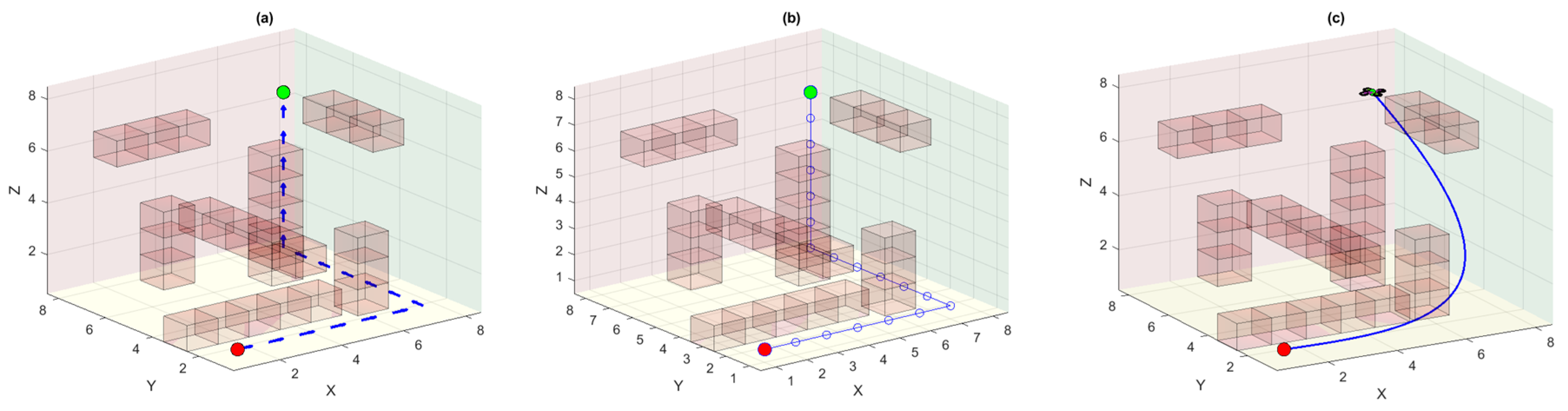
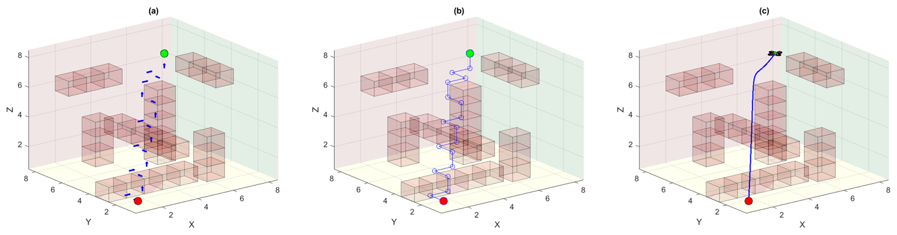
Figure 3 shows the MDP environment of the DQN-based UAV agent where the obstacles are bad states and yield penalties if collisions occur. Similarly, we also have start and goal states in this environment and reaching the goal state yields a higher positive reward. Part (a) of
Figure 3 shows the optimal policy learned by the DQN agent after the Q-actions converge to their final values. Notably, there could be many other optimal policies in this 3D environment that can render a similar distance cost based on the number of steps. Due to the stochastic nature of MDP, the agent may pick any random but optimal policy from these possible optimal policies. However, all these optimal policies render different UAV trajectories even though some have a much reduced path length due to truncation of redundant waypoints. The linear waypoint trajectory for the quadrotor UAV is shown in part (b) of the same figure. As the quadrotor is a second-order system, therefore, it cannot traverse this trajectory having infinite curvature. The trajectory computed using the differential flatness theorem is followed smoothly by the quadrotor UAV and is shown in part (c). However, this is obvious from the figure that this trajectory is not the most optimal trajectory as there exists almost a direct straight-line trajectory between the start and the goal points (see
Section 4.4).
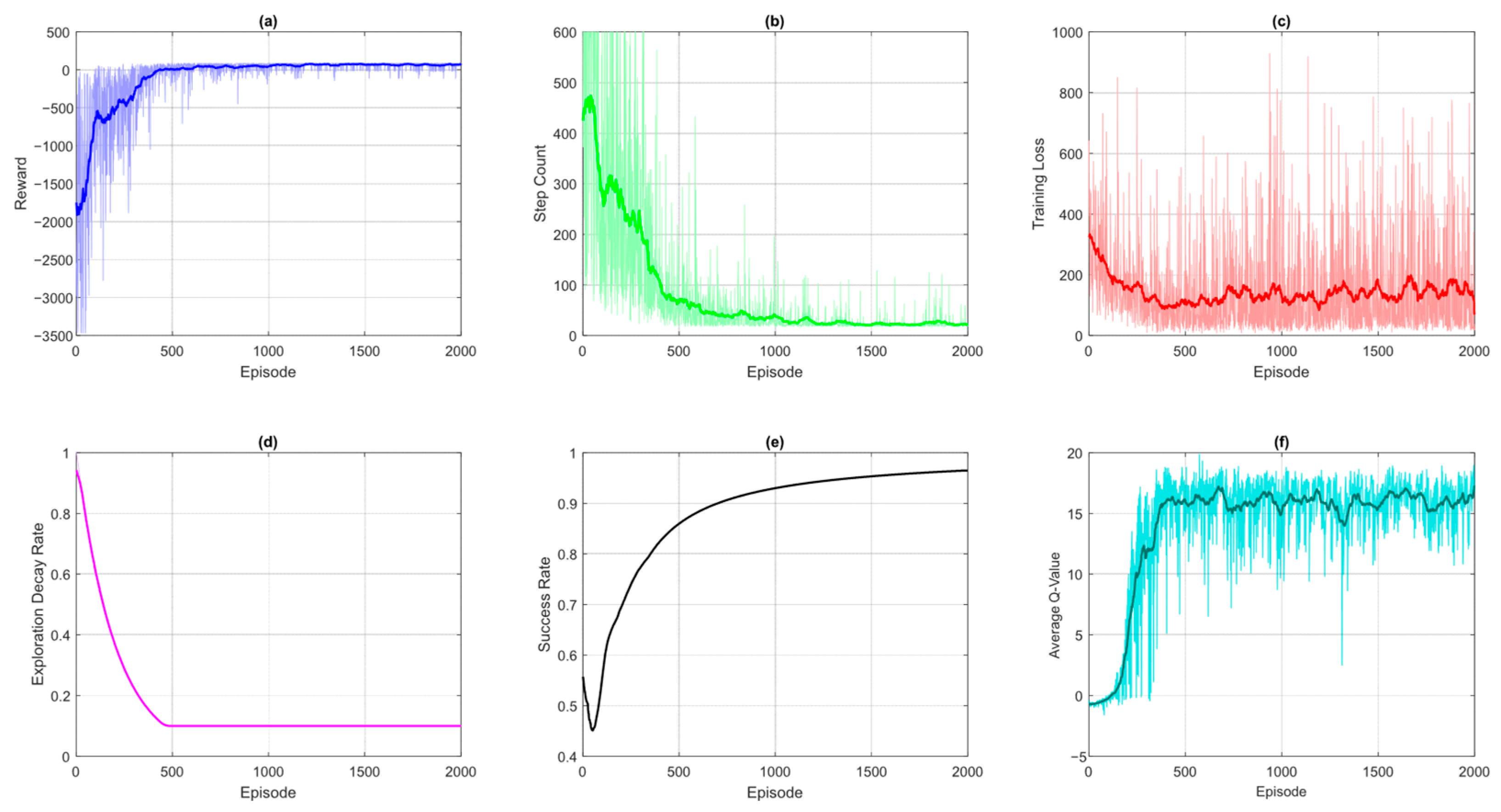
The learning dynamics and performance of the DQN-based UAV navigation system can be comprehensively analyzed through several key training curves with each providing unique insights into different aspects of the algorithm’s behavior.
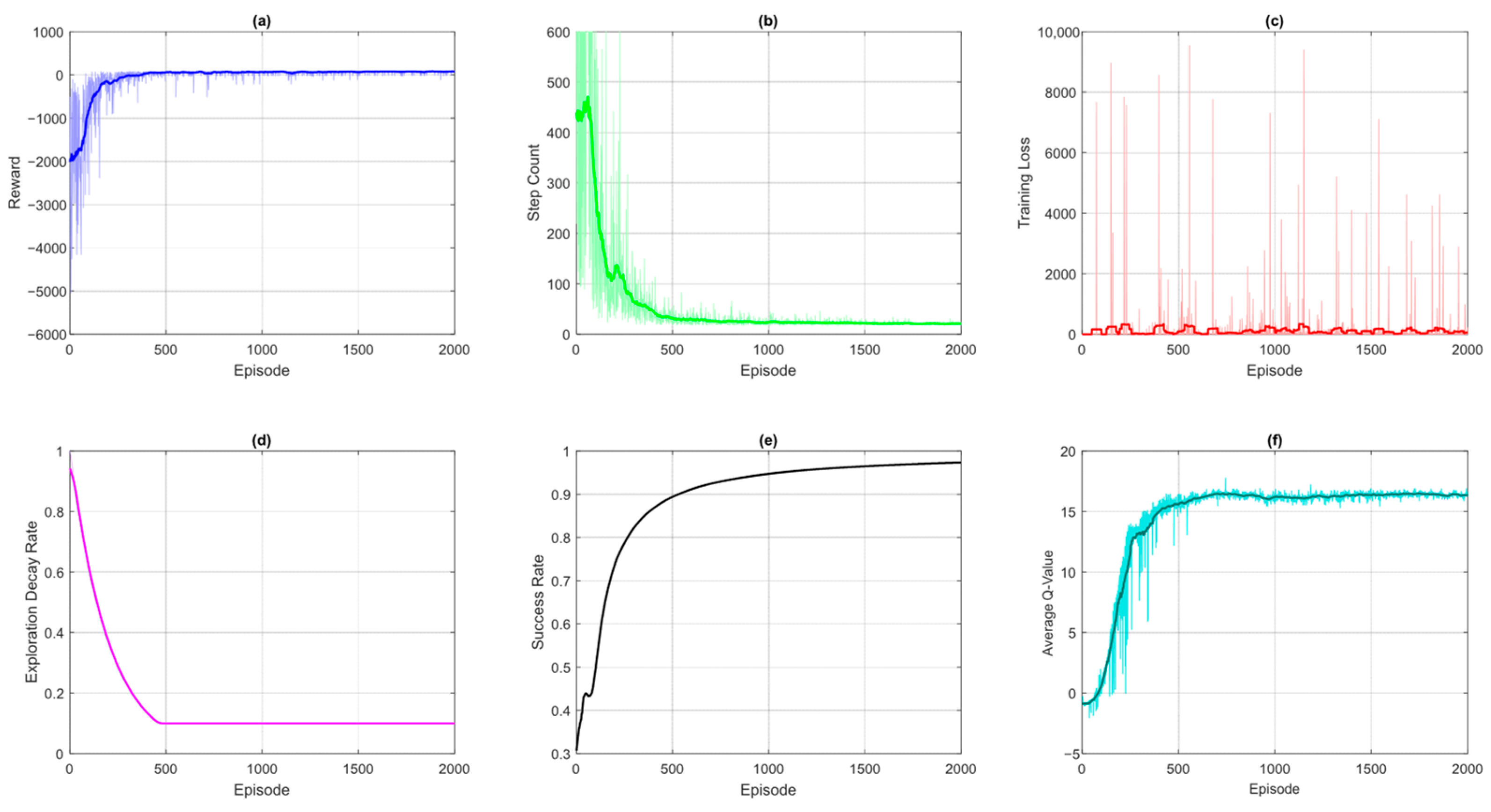
Figure 4 shows curves of various metrics obtained after the implementation of the DQN algorithm for UAV path planning. Part (a) depicts the cumulative reward obtained by the agent and serves as the primary indicator of overall learning progress. The increasing trend demonstrates the agent’s improving ability to maximize cumulative rewards while plateaus suggest policy convergence. Initial high variance reveals instability in training due to higher initial exploration. Part (b) demonstrates the steps per episode curve which measures the path-finding efficiency. The decreasing number of steps indicates the DQN-based UAV agent is learning shorter and more optimal trajectories to the goal. The occasional spikes reflect temporary failures due to exploration or environmental complexity. Part (c) depicts the training loss, and it reveals how well the neural network approximates the true Q-values. An initial high loss is as per expectation due to random weight initialization. The training loss curve follows a declining trend as the network learns gradually. This leads to higher cumulative rewards and reduced variance in performance, as the UAV generalizes better across states. The spikes and oscillations indicate issues like overly aggressive learning rates and the absence of sufficient experience replay.
Meanwhile, the exploration decay rate demonstrated in plot (d) tracks the balance between exploration and exploitation, which shows how the ε-greedy strategy transitions from predominantly random actions to Q-value-driven decisions. The low epsilon value ensures continued exploration even during the late stage of the DQN training. The success rate curve shown in part (e) of
Figure 4 quantifies the reliability of the DQN agent by measuring the percentage of episodes where the goal is reached. The increasing trend of the curves indicates that the agent gradually learns better policies and reaches the goal more frequently. However, the success rate of DQN is around 90 percent which can still be improved. Part (f) of
Figure 4 depicts the average Q-values curve and provides a window into the agent’s confidence in its actions. The rising values reflect improving policy quality and convergence of the DQN agent to the final and optimal solution in terms of Q-values.
4.2. Case 2 DQN-ER
In contrast, DQN with experience replay utilizes a replay buffer to uniformly sample past transitions which effectively reduces the temporal correlation inherent in sequential decision-making. This enhancement leads to more stable training dynamics and improved convergence speed compared to the baseline DQN. This is because the agent learns from a more diverse and uncorrelated set of experiences. However, uniform sampling may still overlook rare but critical experiences, such as near-collision states and high-reward transition. This may limit the ability of the algorithm to refine its policy efficiently in complex scenarios.
Figure 5 shows the MDP-based UAV environment with the DQN-ER algorithm for path planning. The learned random but optimal policy by the DQN-ER agent is shown in part (a). Again, there could be several other optimal policies each having the same distance cost function but may generate different suboptimal UAV trajectories. This scenario again demands the need to enable the UAV agent to learn or select such an optimal policy that could ultimately generate the best and optimal trajectory. Parts (b) and (c) show the linear waypoint trajectory, and the smooth and dynamically feasible trajectory based on differential flatness theory, respectively. The quadrotor UAV efficiently tracks the generated trajectory based on the waypoints received by the DQN-ER planner.
The DQN-ER demonstrates superior performance over the baseline DQN across all key training metrics which reflects its enhanced stability, efficiency, and learning robustness.
Figure 6 shows the metric plots obtained using the DQN with the experience replay mechanism. From
Figure 5, we have seen there is not any improvement in the UAV final trajectory due to the stochastic nature of the algorithm. However, the metric plots of DQN-ER shown in
Figure 6 are better as compared to baseline DQN plots. This quantifies the efficient use of the experience replay mechanism in the traditional DQN approach.
The cumulative reward obtained by the UAV agent using DQN-ER as shown in part (a) has less initial variance and convergence to final rewards is fast, smoother, and has more consistent ascent. This is due to the replay buffer that mitigates the correlation between consecutive updates and allows the agent to learn from a diverse set of past experiences rather than just recent transitions. This leads to higher cumulative rewards and reduced variance in performance, as the UAV generalizes better across states. Similarly, the steps-per-episode curve as shown in plot (b) of the same figure depicts a steeper decline that indicates that the agent discovers more efficient navigation paths earlier in training. Contrarily, the baseline DQN often struggles with erratic step-counts due to overfitting to recent experiences. The randomized sampling smooths out learning and enables the UAV to converge to optimal trajectories more reliably. Similarly, the training is much better due to more consistent gradient updates as shown by the minimal training loss curve depicted in plot (c).
The higher spikes are due to the random sampling of diverse target values from past experiences. The exploration decay rate is kept the same in all experiments. Meanwhile, the success rate curve rises more rapidly and reaches a higher plateau in DQN-ER, as the agent leverages a broader range of experiences to overcome challenging states (e.g., obstacle-dense regions). Finally, the average Q-value curve in DQN-ER shows steadier growth with fewer signs of overestimation as the diversified training batches lead to more accurate value estimates. On the contrary, the baseline DQN is prone to overfitting to noisy Q-value targets due to lacking experience replay which ultimately results in erratic spikes.
4.3. Case 3 DQN-RS
Another variant of the baseline DQN incorporates reward shaping to mitigate the challenge of sparse rewards. By introducing auxiliary feedback signals, reward shaping guides the UAV toward more desirable behaviors and improves policy learning. This technique is expected to significantly accelerate early-stage learning by providing the agent with more frequent and informative reward signals. However, improperly designed reward function introduces bias which may lead the UAV agent to exploit shaped rewards at the expense of the true objective. For instance, excessive penalties for minor deviations may discourage exploration, while overly optimistic shaping could result in locally optimal but globally subpar trajectories. Careful tuning is essential to ensure that the shaped rewards align with the true goal of reaching the target efficiently. It is evident from
Figure 7 that the policy learned by the UAV agent using the DQN-RS algorithm is again rendering a suboptimal trajectory for UAV tracking. Although reward shaping has improved the other training metrics as shown in
Figure 8, the policy is still random, and the UAV agent needs to learn those policy actions that ultimately could generate the most optimal trajectory.
4.4. DQN-Proposed
The proposed hybrid approach, combining PER, L2 regularization, and incorporating modified tie-breaking mechanisms, outperforms the other variants in both learning efficiency and final policy rendering. PER ensures that high-TD-error transitions that have the most significant learning potential are sampled more frequently. This helps in accelerating convergence in critical states and overcomes the issues of simple ER. L2 regularization alleviates overfitting by penalizing excessive weights and promotes generalization across unseen grid configurations, while the modified tie-breaking strategy prevents the agent from oscillating between equally valued actions. The effective tie-breaking mechanism adopted in the proposed approach renders only that policy that subsequently generates the best and optimal UAV trajectory. Together, these components produce a policy that not only learns faster but also achieves higher cumulative rewards. Moreover, it also navigates the 3D obstacle-cluttered environment with greater reliability than the baseline and intermediate variants. The results demonstrate a smoother and more stable ascent in reward curves. Meanwhile, the UAV consistently avoids local optima and converges to near-optimal paths.
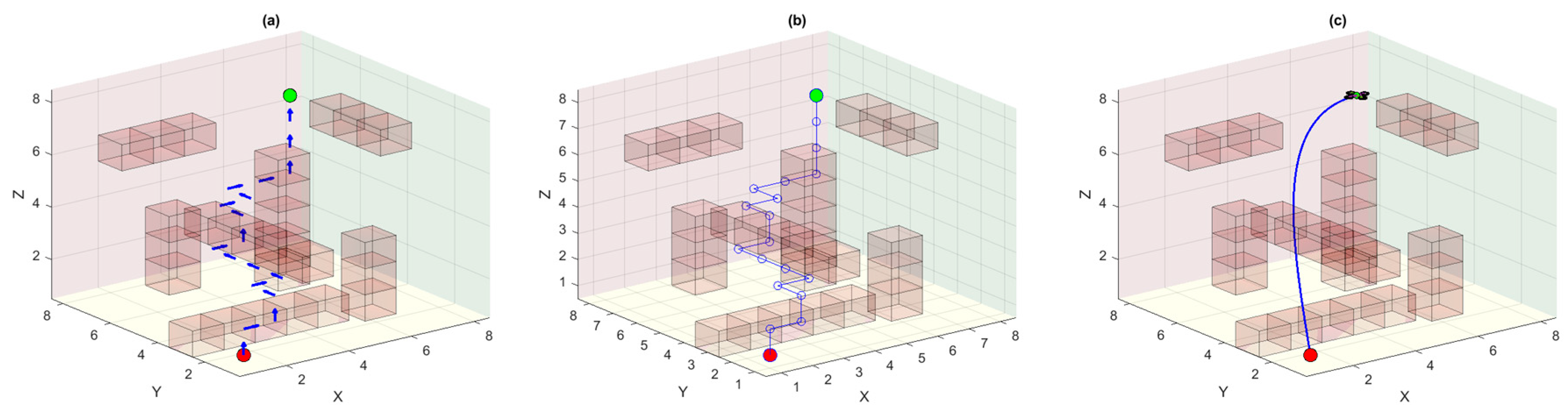
Figure 9 (part a) shows the improved policy learned by the UAV agent using the proposed DQN algorithm. We see the policy arrows are more directed towards the actual goal. From part (b), we can see the waypoint trajectory which has the same cost function as was in all previous cases. However, the trajectory generated from these waypoints is more optimal as compared to other trajectories that were computed previously. The proposed approach effectively reduces the trajectory length and ultimately enhances the endurance of the UAV.
From the training metrics demonstrated in
Figure 10, we can see the improved performance of the proposed algorithm. The reward-per-episode curve in part (a) demonstrates a faster initial rise and higher asymptotic performance compared to other variants, as PER ensures critical transitions (e.g., obstacle avoidance or goal achievement) are replayed more frequently. In contrast, the baseline DQN suffers from slow convergence due to sparse rewards, DQN-ER lacks focus on high-impact experiences, and DQN-RS introduces bias which may lead the UAV agent to exploit shaped rewards at the expense of the true objective. The steps-per-episode curve shown in part (b) reveals that our proposed approach achieves optimal paths sooner and with fewer outliers, as PER efficiently propagates knowledge from pivotal moments and the proposed tie-breaking mechanism efficiently picks the best action from the equally valued actions. While DQN-ER and DQN-RS improve over the baseline, they still miss PER’s targeted learning and perform relatively worse. The training loss curve in part (c) shows smoother and more stable convergence in our proposed method. The PER focuses on high-TD-error transitions which reduce variance in updates. Meanwhile, the baseline and DQN-ER exhibit noisier loss curves, and DQN-reward shaping overfits to shaped rewards without PER’s balancing effect.
Critically, the success rate curve of our proposed approach (demonstrated in part (e)) climbs more rapidly and reaches a higher peak of 100 percent after 1500 episodes. All other DQN variants could not achieve 100 percent success rate even after 2000 episodes. This shows the superiority of our proposed approach. Finally, the average Q-value curve in part (f) reflects more accurate, faster, and stable value estimates. PER corrects overestimations through focused replay, and the tie-breaking mechanism accurately selects the policy actions for equally valued actions. In contrast, other variants either suffer from biased estimates (baseline), uniform sampling inefficiencies (DQN-ER), or shaping-induced local optima (DQN-RS).
4.5. Discussion and Comparative Analysis
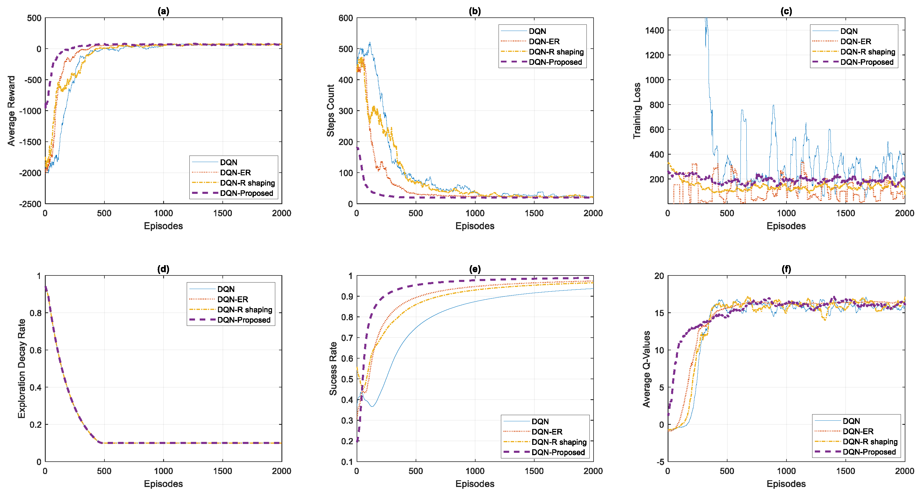
Figure 11 shows the comparative results of our proposed DQN approach with baseline DQN and all other variants. We can see in part (a) the average reward curve of our proposed DQN approach is faster, smoother, and has less variance as compared to other variants which shows the effectiveness and superiority of our method. Similarly, in part (b) the convergence of steps count curve of our proposed approach outperforms all other methods which again shows the validation of the superiority of our method. In part (c), the training loss curve of our method shows less perturbations due to less variance and is more stable comparatively. Part (d) shows the exploration decay rate which is kept the same for all the experiments. The comparative success rate graphs of all the methods in part (e) again verify that the proposed DQN approach has significant advantages over other methods. Similarly, the average Q-values converge quickly and smoothly in our proposed approach and again verify that our proposed method outperforms all other methods.
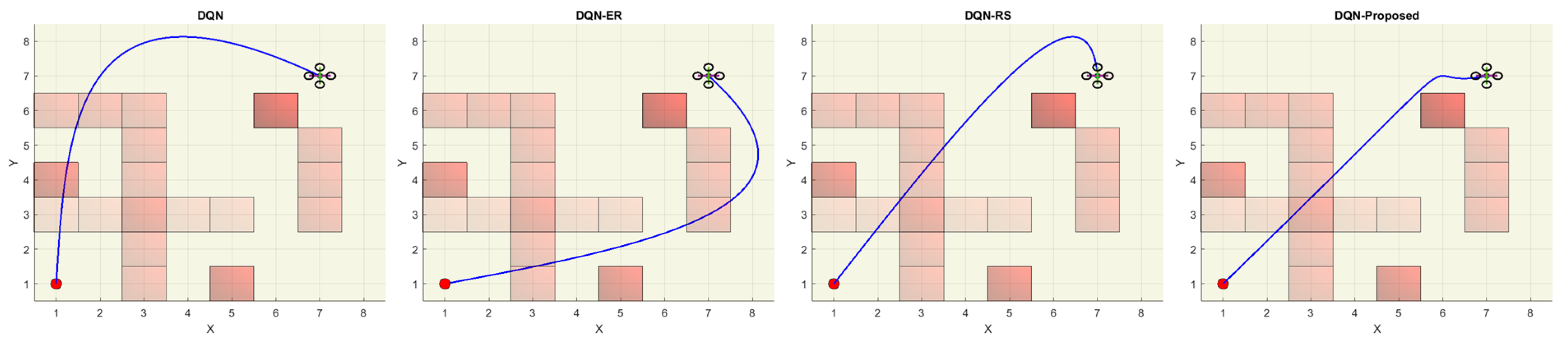
Figure 12 demonstrates the top view of all the trajectories that were followed by the UAV, and it is obvious from this view that our proposed method generated the most optimal trajectory which is almost a straighter line from start to goal position. The same has been conferred by
Figure 13 where we have calculated the trajectory lengths of all the trajectories followed by the UAV under various simulation experiments. The path obtained by our proposed method generates the shortest UAV trajectory which is about 10.72 grid units.
Collectively, the simulation results demonstrate that our proposed DQN approach consistently outperforms the baseline DQN, DQN-ER, and DQN-RS across all evaluated metrics. By integrating prioritized replay, the agent learns more efficiently from high-impact transitions. The incorporation of L2 regularization in the proposed DQN framework plays a pivotal role in enhancing the stability and generalizability of the learning process. By adding a penalty term proportional to the squared magnitude of the network weights to the loss function, L2 regularization effectively prevents the neural network from overfitting to noisy and sparse reward signals, which is particularly crucial in the UAV navigation task where environmental states and rewards can be highly variable. This regularization ensures that the Q-values remain conservative and robust and mitigates the risk of over-optimistic predictions that could destabilize training. The addition of tie-breaking further refines exploration and prevents convergence to those policies which render sub-optimal UAV trajectories. Together, these enhancements lead to faster convergence, higher success rates, and more stable training dynamics which are evidenced by the superior reward curves, reduced step counts, and smoother loss profiles. These findings validate the robustness of our framework for UAV navigation in complex 3D environments and suggest broader applicability to other reinforcement learning tasks which require precise, adaptive decision-making. A detailed video animation of our presented work can be found as
Supplementary Material (see
Video S1).
The proposed DQN-based framework, although validated in a simulated 3D cluttered environment, is developed with a strong emphasis on real-world applicability and deployment feasibility. In real-world scenarios, the trained policy can be integrated into physical UAV platforms equipped with onboard sensors such as GPS, IMUs, and depth or LiDAR sensors for environment perception and state estimation. The discrete high-level actions generated by the DQN agent can be translated into low-level control commands using a trajectory tracking or waypoint-following controller. Additionally, key real-world challenges including sensor noise, localization errors, actuator delays, and dynamic environmental changes must be addressed during deployment. To bridge the gap between simulation and physical testing, our future work will focus on hardware-in-the-loop simulations and field experiments to evaluate the robustness and adaptability of the proposed method in uncontrolled and partially observable environments.
5. Conclusions
In this work, an improved deep Q-learning framework has been proposed to address the limitations of traditional DQN-based reinforcement learning in UAV path planning within complex 3D environments. The proposed framework incorporates a modified tie-breaking mechanism to avoid suboptimal local decisions, prioritized experience replay to enhance sample efficiency, and L2 regularization to improve training stability. The improved learned policy promotes optimal flight paths and ultimately generates smoother and optimal UAV trajectory. The results demonstrate that the combined use of these techniques leads to significantly improved navigation performance compared to baseline methods. Specifically, as demonstrated in the results section, the proposed approach has significantly reduced the trajectory length due to its more efficient and informed action-selection mechanism. Moreover, across multiple performance metrics including average reward, step count, training loss, success rate, and average Q-values, the proposed method has consistently outperformed all other DQN variants. These improvements reflect faster convergence, more stable learning dynamics, and enhanced policy effectiveness in navigating complex 3D environments. The proposed framework provides a reliable and scalable solution for autonomous UAV navigation in cluttered spaces and lays the groundwork for further research in real-world deployment and multi-agent coordination scenarios. Future work could also explore dynamic reward shaping and hybrid exploration strategies to further optimize performance. Additionally, we plan to extend this research to real-world UAV experiments. In a physical setup, factors such as sensor noise, hardware limitations, real-time processing delays, and environmental disturbances (e.g., wind or GPS inaccuracies) are expected to influence navigation performance. Addressing these challenges will be essential to successfully transferring the proposed approach from simulation to practical deployment.


 ,
, 


