Visual Point Cloud Map Construction and Matching Localization for Autonomous Vehicle

Abstract

Collaboration between autonomous vehicles and drones can enhance the efficiency and connectivity of three-dimensional transportation systems. When satellite signals are unavailable, vehicles can achieve accurate localization by matching rich ground environmental data to digital maps, simultaneously providing the auxiliary localization information for drones. However, conventional digital maps suffer from high construction costs, easy misalignment, and low localization accuracy. Thus, this paper proposes a visual point cloud map (VPCM) construction and matching localization for autonomous vehicles. We fuse multi-source information from vehicle-mounted sensors and the regional road network to establish the geographically high-precision VPCM. In the absence of satellite signals, we segment the prior VPCM on the road network based on real-time localization results, which accelerates matching speed and reduces mismatch probability. Simultaneously, by continuously introducing matching constraints of real-time point cloud and prior VPCM through improved iterative closest point matching method, the proposed solution can effectively suppress the drift error of the odometry and output accurate fusion localization results based on pose graph optimization theory. The experiments carried out on the KITTI datasets demonstrate the effectiveness of the proposed method, which can autonomously construct the high-precision prior VPCM. The localization strategy achieves sub-meter accuracy and reduces the average error per frame by 25.84% compared to similar methods. Subsequently, this method’s reusability and localization robustness under light condition changes and environment changes are verified using the campus dataset. Compared to the similar camera-based method, the matching success rate increased by 21.15%, and the average localization error decreased by 62.39%.

1. Introduction

In three-dimensional transportation systems, autonomous vehicles play a crucial role [1], exemplified by their collaboration with drones to optimize traffic flow and enhance logistics efficiency. The global navigation satellite system (GNSS) can provide accurate and drift-free localization data, but becomes inoperative in signal obstruction or complete loss [2]. When satellite signals are unavailable, co-operative navigation for drones and vehicles has become a significant development trend. The motion modality of ground autonomous vehicles is relatively stable, and they can acquire rich and detailed environmental information, enabling high self-contained localization accuracy [3]. Therefore, autonomous vehicles often serve as anchor nodes, providing auxiliary localization information to drones within the co-operative navigation system [4], making precise and robust vehicle localization critical.

In situations where satellite signals are unavailable, most existing localization solutions rely on visual odometry (VO) or LiDAR odometry (LO) [5,6]. However, minor matching errors between frames accumulate as driving time and distance increase, resulting in the drift in localization accuracy [7]. Simultaneous Localization and Mapping (SLAM) techniques can utilize loop closures to correct odometry localization drift errors. Nevertheless, closed loops may not always exist, leading to correction failures [8]. Integrating multiple sensors for localization is also a common solution, but relative sensors like wheel and inertial sensors cannot fundamentally suppress drift errors [9]. Absolute sensors such as altimeters and compasses are easily influenced by electromagnetic interference, with limited application scenarios [10,11].

Under the requirements of the three-dimensional transportation system navigation, the localization system needs to provide geographically absolute pose estimation. Matching environmental landmarks and prior digital maps has become an effective localization method when satellite signals are unavailable [12]. Among these, the acquisition of high-precision maps and the achievement of accurate matching localization are the main research focuses [13]. The primary external sources of digital maps are public platforms [14], and data are usually packaged in fixed formats, with limited usability, and cannot be autonomously updated. In practical applications, researchers usually need to construct specific digital maps based on the demand for matching localization. Intelligent map construction methods based on LiDAR SLAM [15] and Visual SLAM [16] have gained widespread adoption, offering significant advantages over traditional mapping techniques. However, they are limited by map accumulation errors [17]. LiDAR provides ranging data and can construct accurate dense point cloud maps [18]. Matching real-time LiDAR scans to these maps has exhibited excellent localization performance [19]. Nevertheless, LiDAR is both expensive and bulky, and its ranging capabilities can be partially supplanted by stereo cameras [20]. Using LiDAR for map construction while equipping the vehicles with cameras for localization can effectively reduce the weight and cost of vehicle-mounted sensors [21]. However, data density and modality differences between LiDAR and camera can decrease matching accuracy and even lead to localization failures [22].

Based on this, this paper proposes a visual point cloud map construction and matching localization method for autonomous vehicles. When satellite signals are available, we propose the Satellite-Assisted Visual Point Cloud Map Construction (SAMC) method, which introduces absolute location constraints to assist in constructing the geographically high-precision VPCM. In situations where satellite signals are unavailable, we propose the corresponding Prior-Map-Constrained Localization (PMCL) method, which introduces constraints by matching the local point cloud with the prior map to suppress the cumulative errors of the odometry, providing stable and accurate location estimates. The experiments carried out on the KITTI and campus datasets demonstrate the effectiveness and accuracy of the proposed map construction method and localization approach.

The remaining part of this paper is organized as follows. Section 2 introduces the related work. Section 3 provides an overall overview of this system. Section 4 details the prior visual point cloud map construction method. The method of map matching and fusion localization algorithm are introduced in Section 5. Section 6 presents the experimental results. Conclusions are given in Section 7.

2. Related Work

Relocalization is an important function of SLAM, which can locate the vehicle in case of tracking failure. At the broader application level, by pre-constructing the digital map, we can utilize the relocalization technique to accurately locate the vehicle within the map to complete navigation tasks.

2.1. Map Construction

Map acquisition platforms primarily include public map websites [23] and map companies [24]. Generally, maps from external sources are packaged in specific formats mainly for displaying location information, which cannot meet map matching and localization requirements. Traditional methods require professionals to collect raw data using specialized equipment and construct the map after the complex data processing. Challenges such as high workload, high maintenance costs, and long update cycles exist. Intelligent map construction methods have become mainstream with the rapid development of geodesy, sensors, and multi-source fusion localization technologies [25].

Map automation construction methods based on SLAM technology are extensively utilized. Compared to LiDAR, cameras have the advantages of low cost, lightweight, and ease of hardware setup, making them more practical for use in vehicles [26]. Visual SLAM is primarily categorized into direct and feature-based localization methods [27]. The former has good real-time performance but is not as robust regarding the angle of view and lighting changes. Simultaneously, loop detection and relocalization in direct methods also rely on features. Overall, feature-based Visual SLAM systems are more suitable for constructing digital maps for matching localization [28]. However, construction methods based on SLAM are limited by map accumulation errors.

The construction of the complete regional map is typically decomposed into the construction and fusion of multiple sub-maps. The authors of [29] propose a simultaneous localization and multi-mapping method, which constructs the new sub-map in case of tracking failure. Each sub-map is independently stored, and the connections are loose without forming a complete global map. The authors of [30] detect loops between the sub-maps constructed at different times and merge them into the primary map. Both of the above methods fix the relative reference frame to the initial frame of the specific sub-map and cannot provide global information for matching localization.

2.2. Matching Localization in Prior Map

The localization methods based on map matching mainly include LiDAR-based, LiDAR-camera-fused, and camera-based methods.

LiDAR-based methods primarily leverage the geometric characteristics of objects and structures within the environment. The authors of [31] design the Extended QuadTree model that can efficiently compress map storage space. Wen et al. introduce the Bursa linearized model to accelerate the matching speed during the iterative process. The authors of [32] use LiDAR SLAM to generate the local 3D map. A Siamese-structured place recognition network correlates and matches landmark information between the local 3D map and publicly available 2D maps to locate vehicles.

The above LiDAR-based methods have excellent localization performance. Nonetheless, LiDAR systems are both pricey and unwieldy. To decrease the weight and cost of the navigation system, researchers acquire public LiDAR point cloud maps and use cameras for vehicle localization. The authors of [33] use the stereo camera disparity map, and the camera pose is estimated through the minimization of depth residuals. This approach has a fast matching speed but becomes ineffective in areas with limited structural information. The authors of [34] propose a monocular visual localization system based on cross-modal registration. A point-to-plane Iterative Closest Point algorithm is designed, and a decoupling optimization strategy is proposed to align the point clouds from the vision and LiDAR map. The authors of [35] associate and register the vehicle’s local semantic object map with a compact LiDAR semantic reference map to achieve localization.

The LiDAR-camera-fused methods are limited by the source of maps, making supplementation and updates impossible. Additionally, the data acquisition methods of LiDAR and camera differ significantly in the field of view and resolution, increasing the probability of matching failures. In contrast, camera-based methods have higher map autonomy and matching robustness, primarily divided into high-definition map matching, photometric feature matching, and geometric feature matching. The authors of [36] design the visual odometry based on Squared Planar Markers (SPM), which can accurately locate the camera in the pre-built SPM map. However, the SPM map requires personnel to set up and maintain. It is only suitable for small-scale fixed environments. High-definition maps contain comprehensive environmental image information but often fail to provide accurate vehicle pose estimates. The authors of [37] propose a monocular visual-inertial SLAM system that supports sub-map merging. This system utilizes photometric feature matching to locate the camera within the pre-built map. However, the maps constructed suffer from cumulative error and lack absolute geographical localization data. To tightly couple semantic and structure information from prior maps, the authors of [38] present a hybrid constraint using the Dirichlet distribution. Then, with the local landmarks and their semantic states tracked in the frontend, the camera poses and data associations are jointly optimized through the Expectation-Maximization algorithm for accurate localization in a prior semantic map. The authors of [39] construct the global photometric feature map based on the Visual SLAM algorithm and real trajectory data, which can locate the camera in the geographical coordinate system. The photometric feature map’s main shortcoming is the lack of robustness to the lighting changes. Churchill et al. store maps of the same location at different times to locate the vehicle [40], but cannot fundamentally solve the problem of changing lighting conditions over time. Comparatively, the geometric features have stronger stability and are unlikely to change significantly in the short term. The authors of [41] employ the SGBM algorithm to construct real-time visual point clouds and achieve precise localization through NDT transformation and matching with the pre-built map. This method is based on environmental geometric features and exhibits strong robustness. However, the visual point cloud map construction relies on LiDAR’s assistance.

To address the shortcomings of the above methods, this paper proposes a visual point cloud map construction and matching localization method for autonomous vehicles. The SAMC method antecedently constructs the regional high-precision VPCM through the fusion of multi-sensor information. In situations where satellite signals are unavailable, the PMCL method introduces the global pose constraints by matching real-time point clouds and the prior map, which can correct the odometry errors and enhance vehicle fusion localization accuracy. The main contributions of this paper are as follows:

• The designed model of the visual point cloud map can extract features from complex raw data and provide enough data support for matching localization. By introducing the road network base, this model achieves effective regional segmentation, which can accelerate the data indexing speed of the matching localization process.
• A multi-sensors fusion map construction method is designed, which lies the enforced constraints of inverse external parameters. This method can autonomously build geographical high-precision visual point cloud maps.
• An improved iterative closest point matching method is proposed to reduce the impact of local convergence, which can effectively enhance the success rate of matching and localization accuracy.
• The proposed fusion localization strategy based on pose graph optimization can reduce the mismatch rate of point cloud matching, effectively constrain the drift error of odometry, and enhance vehicle localization accuracy.

3. System Overview

This paper assumes that the satellite signals are unavailable, which leads to the GNSS being unable to provide position information for the in-vehicle navigation system. Based on historical localization data, we can determine the accurate initial position of the vehicle and load the pre-built regional VPCM. Meanwhile, the attitude angle of the vehicle can be measured using the electronic compass. Due to significant interference from other electronic devices during driving, the output data of the electronic compass will not be used for subsequent localization. We turn on the visual odometry for navigation, continuously introducing constraints from the prior VPCM to suppress cumulative error and output fusion localization results.

This paper proposes a visual point cloud map construction and matching localization method for autonomous vehicles. The overall framework of the system is illustrated in Figure 1, which is divided into two temporal phases: prior map construction and navigation localization. During the map construction phase, i.e., the “free time” when satellite signals are available. Network Real-Time Kinematic (NRTK) [42] can provide global high-precision drift-free positioning data. The SAMC method fuses it to the Visual SLAM system, which can effectively suppress cumulative error while providing absolute geographical reference to the SLAM-constructed relative map.

During the navigation localization phase, the satellite signals are unavailable. The vehicle turns on the visual odometry to provide initial pose estimation, which helps adaptively segment the prior VPCM. The PMCL method matches the extracted local point cloud with the reference map to provide the absolute pose estimation of the vehicle. The two complement each other. Visual odometry estimates the relative pose of the vehicle, while the accumulated error can be effectively constrained by the absolute pose obtained through point cloud matching. Simultaneously, the initial pose calculated by the odometry can prevent localization errors caused by mismatch and localization information loss due to matching failures.

4. Visual Point Cloud Map Construction

ORB-SLAM2 [43] is a classic open-source Visual SLAM algorithm based on keyframes, consisting of four threads: tracking, local mapping, loop detection, and loop correction. The visual feature ORB corners used in this system exhibit good invariance to rotation, scale, and lighting changes. ORB-SLAM2 serves as the foundation of the mapping method designed in this paper. The SAMC method utilizes its corner extraction, feature matching, spatial position recovery, and other essential components under the stereo camera model, fuses NRTK data, and constructs the global drift-free visual point cloud map in the georeferenced coordinate system.

4.1. Visual Point Cloud Map Model

Traditional Visual SLAM matches the features between adjacent frames to track the vehicle and construct the photometric feature map. Utilizing feature descriptors can achieve high accuracy matching during the localization process without requiring a precise initial vehicle pose. However, the success rate of matching photometric features decreases quickly in situations with significant variations in environmental lightness, and the high dimensionality of descriptors also burdens storage space.

In contrast, the geometric structure of the environment is more stable. The same location may look different due to changes in lightness, but the geometric structure is unlikely to change. At the same time, the geometric structure only requires spatial location information of the map points, leading to lower storage space requirements. However, geometric structure matching for localization requires good initial pose estimation. Otherwise, it may easily fall into long search times or local optimum, leading to increased matching time, decreased matching success rate, and reduced localization accuracy.

Based on this, we design a new visual point cloud map model, which includes the regional road network base, the trajectory of the keyframes during the mapping process, and geometric point clouds around the roads. Specifically, it includes (1) the point-line form road network, which assists in dividing point clouds and accelerates data indexing during the matching process; (2) the six-degree-of-freedom poses of the keyframes, which are used to increase the success rate of point cloud matching; (3) the three-degree-of-freedom spatial positions of the point clouds, which are used to ensure map applicability at different times and reduce required storage capacity.

4.2. Road Network Base Construction

Even when changes occur in the surrounding environment of the roads, the structure of the road network remains almost unchanged, showcasing its long-term stability. The regional road network map required in this paper is the topological map of the point-line form, and the raw data can be obtained through public map websites like OpenStreetMap (OSM). The road network map data mainly consist of two essential elements: nodes and roads. The node element represents the individual sampling point of the road network, including its latitude, longitude, and altitude coordinates. The road element consists of the list of node elements.

The authors of [44] define the smallest indivisible road segment as the road network basic element (RNBE) and propose the corresponding road network model. On this basis, we take the first node element as the fixed origin and convert the regional road network to the East-North-Up geographical coordinate system. Subsequently, we calculate the intersections between different roads and divide them into multiple RNBEs, i.e., the regional road network base. The definition of a single RNBE is given by Equation (1), where $\left\{\right\}$ represents the set of nodes. $T{p}_{Start}$ and $T{p}_{End}$ represent the head and tail turning points. The RNBEs with the same $Tp$ are mutually connected. $\{S{p}_1,S{p}_2,\dots ,S{p}_n\}$ represents the skeleton point group. Sequentially connecting them can approximate the shape of the road.

$$RNBE:=\left\{T{p}_{Start},S{p}_1,S{p}_2,\dots ,S{p}_n,T{p}_{End}\right\}$$

(1)

4.3. Point Cloud Map Construction

The map constructed by VSLAM is located in the world coordinate system in general, i.e., the camera coordinate system of the first frame. Meanwhile, the translational and rotational errors of SLAM methods accumulate as the traveled distance grows. The authors of [39] utilize VSLAM to create the feature-based map, then correct the biases with real trajectory assistance to construct the global map. However, this method does not optimize the states of the features, and the two-step construction process will affect the smoothness of the map. To address the above issues, the SAMC method fuses multi-sensor information to construct the prior map based on enforced constraints of inverse external parameters. When the satellite signals are available, the NRTK data are fused into the mapping process to constrain the cumulative error. Furthermore, we design the new error terms to optimize the states of keyframes and features synchronously, ensuring the consistency of the map.

The SAMC method extracts the ORB corner points from stereo image frames and computes the corresponding descriptors. The disparity between the left and right images is used to recover the spatial positions of the corner points for initialization. As shown in Figure 2, during the tracking process, we predict the vehicle’s pose based on the constant velocity model and NRTK data to calculate the relative transformation between frames. On this prediction basis, we project the local map points onto the tracking frame and search for the matching points within a localized region. Let the tracking frame index be $j$. The reprojection cost function $E(i,j)$ is shown in Equation (2) for the local $ith$ map point.

$$E(i,j)=‖e_{ij}‖=\Vert u_{ij}-{\displaystyle \frac{1}{z_i}}K{T}_{wj}^c{P}_i\Vert$$

(2)

where $\Vert \Vert$ represents Euclidean norm, $u_{ij}$ represents the pixel coordinates of the $ith$ spatial point’s matching point in frame $j$, $K$ denotes the intrinsic parameters of the camera, $T_{wj}^c$ represents the pose of frame $j$, $P_i$ signifies the $ith$ spatial point’s position in the world coordinate system, and $z_i$ denotes the depth of point $P_i$ along the camera’s optical axis in the camera coordinate system.

Traditional VSLAM selects keyframes for local bundle adjustment and synchronously optimizes the keyframes’ poses and the map points’ positions. The system typically inserts a new keyframe when the backend is idle to ensure real-time performance. In special cases, to maintain tracking and relocalization performance, the system may interrupt the backend optimization process and forcefully insert a new keyframe, decreasing overall keyframe trajectory and point cloud accuracy. The map can be constructed in advance over a long time before localization in the context of this paper. In the absence of real-time constraints, we extract all image frames as keyframes to participate in backend optimization, which can enhance the overall accuracy and density of the map. The tracking process continues after local map optimization is completed.

In the system backend, we optimize keyframes $K_L$ that have mutual visibility with the real-time keyframe (able to observe the same map points), along with the map points $P_L$ observable by these keyframes. All other keyframes $K_F$, not in $K_L$, observing points in $P_L$ contribute to the cost function but remain fixed in the optimization. In addition to the reprojection error, the SAMC method introduces the absolute position cost function $E(j)$ from NRTK data, which are shown in Equation (3), where $O_{wj}$ represents the position of the camera at time $j$ in the world coordinate system, while $P_{gj}$ represents its position at the same time in the geographical coordinate system. $t_{cj}^w$ is the translation component of $T_{cj}^w$, and $T_g^w$ is the transformation matrix.

$$E(j)=‖e_j‖=\Vert O_{wj}-T_g^w{P}_{gj}\Vert =\Vert t_{cj}^w-T_g^w{P}_{gj}\Vert$$

(3)

As shown in Equation (2), the reprojection error constrains $T_w^c$ and the NRTK data constrain $t_c^w$, i.e., the translation component of $T_c^w$. Assigning excessive weight to the reprojection error will diminish the effectiveness of NRTK data, while assigning too much weight to the absolute position error will reduce the spatial accuracy of map points. To balance the two and achieve optimal optimization results, we design the inverse external parameters enforced constraints cost function $E^{\prime }(j)$, where the external parameter of the frame $j$ to be optimized is $T_{wj}^c$, with its inverse matrix being $T_{cj}^w$.

$$E^{\prime }(j)=‖{e^{\prime }}_j‖=‖{\left[ln\left(T_{wj}^c{T}_{cj}^w\right)\right]}^{\vee }‖$$

(4)

Defining $X_j$ as the set of matches between points in $P_L$ and corner points in the keyframe $j$, the overall cost function of backend optimization is shown in Equation (5):

$$C={\displaystyle \sum _{j\in K_L\cup K_F}\left({\rho }_j{e}_j^T{\Omega }_j^{-1}{e}_j+{{\rho }^{\prime }}_j{e^{\prime }}_j^T{{\Omega }^{\prime }}_j^{-1}{e^{\prime }}_j+{\displaystyle \sum _{i\in X_j}\left({\rho }_{ij}{e}_{ij}^T{\Omega }_{ij}^{-1}{e}_{ij}\right)}\right)}$$

(5)

where ${\rho }_{ij}$, ${\rho }_j$, and ${{\rho }^{\prime }}_j$ represent robust kernel functions, ${\Omega }_{ij}$, ${\Omega }_j$, and ${{\Omega }^{\prime }}_j$ denote the covariance matrices. The optimization process is primarily based on image feature point matching, so we set the weight of $e_{ij}$ (in pixels) as the reference value. Variations in ${e^{\prime }}_j$ (in Lie algebra) affect all reprojection points, and its weight is set to the number of reprojection edges to match the constraint magnitude. $e_j$ (in meters) is strongly constrained by ${e^{\prime }}_j$, similarly affecting all reprojection points. Its weight is set to one-tenth of the number of reprojection edges to balance the scale difference between pixels and meters based on the theory of noise variance ratio [45,46]. Using this method, we can effectively balance reprojection and absolute position errors by ensuring the enforced constraints of inverse external parameters. The global optimization factor graph of the point cloud map construction is shown in Figure 3. When the tracking is over, we optimize all keyframes and points of the map and then transform the VPCM into the geographical coordinate system.

4.4. Overall Map Construction

The prior map should cover the regional road network, including the roads themselves and the visual point cloud for localization on both sides of the roads. Based on the geographical RNBE map constructed in Section 4.2, we divide the construction of the regional overall VCPM into the construction and fusion of multiple sub-maps, and the coverage range of each sub-map can be accurately controlled by controlling the start and stop of the multi-sensors fusion mapping system. When significant changes occur in the environmental geometric features, we conduct supplementary mapping for the affected road segments to replace the original map. Similarly, this method can also be used for supplementary mapping of road segments where satellite signals are partially or temporarily lost. This design effectively reduces the coupling between point cloud maps of different road segments and lowers the cost of updating and maintaining.

The SAMC method determines the road segment to which the keyframe belongs based on its geographic location. We extend the rectangular and quadrilateral expansion methods from [44] to the geographical coordinate system, as shown in Figure 4a and Figure 4b, respectively. The point cloud of RNBE is composed of all map points observable by the keyframes belonging to the RNBE. In general, the intersections of the roads often have multiple results of quadrilateral expansions, which overlap each other. The keyframes located here usually belong to multiple RNBEs.

For the same position, the photometric features observed from different directions may vary, making it difficult to identify loop closures. This also applies to geometric features, as different perspectives can cause variations in observed geometric characteristics due to occlusions of environmental objects. Based on this, the prior visual point cloud for the same road segment should consider orientation factors. Each road segment should construct both forward and reverse point cloud maps to meet the data requirements of the localization.

5. Localization Under Prior VPCM Constraints

When satellite signals are unavailable, the PMCL method achieves localization based on images captured by the camera and the pre-constructed VPCM. During this phase, the prior map serves as the reference without considering errors, including potential errors. The localization process is illustrated in Figure 5. The visual odometry receives images and continuously outputs real-time poses (increments) and local point clouds. Global constraints are introduced from the prior map by matching the geometric features of the local point cloud with the adaptively segmented sub-map reference point cloud. A global pose graph optimization problem is constructed to achieve fusion localization, continuously optimizing the historical trajectory, and estimating the optimal real-time vehicle pose.

5.1. Visual Odometry

The reliable initial pose estimation is the first step in locating the vehicle under prior VPCM constraints. Based on the known initial pose of the vehicle, the PMCL method applies the front-end odometry of ORB-SLAM2 to track vehicle motion. The difference is that all frames are extracted as keyframes. During the optimization of the local map, the pose of the real-time keyframe and the spatial positions of map points are effectively corrected, providing the matching source for aligning with the prior VPCM. Matching source $D$ is shown in Equation (6), where $SE(3)$ stands for Special Euclidean Group, representing the set of all rigid body transformations in 3D space, including rotation and translation. ${T_D}_c^w$ denotes the pose of the real-time keyframe $K{F}_D$, and $n_i$ represents the number of spatial map points observed by this keyframe.

$$D=\left\{{T_D}_c^w\in SE(3),d_i | d_i\in {\mathbb{R}}^3,i=1,2,3,\dots ,n_i\right\}$$

(6)

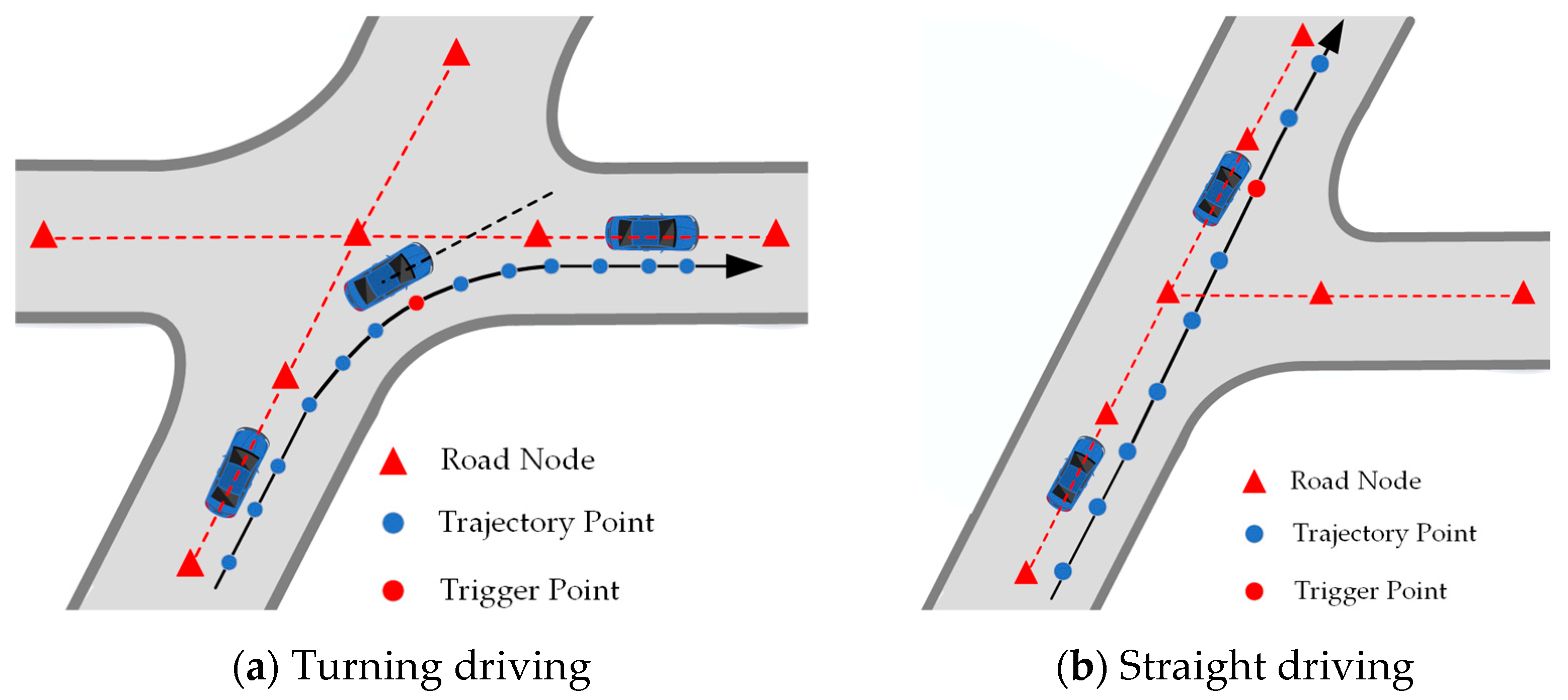
5.2. Adaptive Prior Map Segmentation

Directly matching the local point cloud generated by the odometry with the entire prior VPCM is typically very time-consuming. The PMCL method proposes an adaptive prior map segmentation strategy to accelerate the map matching and localization process. We first locate the road segment to which the vehicle belongs based on its position, and then extract the sub-map from the overall map as the matching reference according to the movement state of the vehicle.

The VPCM model designed in this paper uses the road network as its foundation, associating point clouds with road segments. We adaptively load matching hotspots of the prior VPCM based on the vehicle’s current belonging road segment and predicted trajectory, thereby accelerating the matching speed and reducing the probability of mismatch. When the vehicle approaches the road intersection Tp, we calculate the vehicle’s real-time heading. Once the angle size between the vehicle’s heading and the orientation of the subsequent road segment becomes smaller than the angle size with the orientation of the current road segment, we judge that the vehicle enters the corresponding subsequent road segment, as shown in Figure 6a. On the other hand, if the vehicle moves in a straight line past the road intersection, we will retain the possibility of the vehicle entering other RNBEs due to the existence of localization error until the vehicle exits the intersection area, as shown in Figure 6b. For more complex road network structures, such as roads with similar turning directions following an intersection, it is hard to accurately determine the road segment to which the vehicle belongs with visual odometry localization error. We will retain the possibility of the vehicle located in every road segment, waiting for subsequent accurate geometric matching localization results to determine the specific road segment it belongs to.

After determining the vehicle’s belonging road segment, we load keyframes located within the 100-m range ahead of the vehicle’s real-time position and observed map points as the sub-map matching reference instead of the entire map. The sub-map reference is updated in real-time during the vehicle’s movement to accelerate the matching speed. Visual odometry provides vehicle position in the initial stage, and later position is the fused localization output, which will be introduced in detail in Section 5.4.

When the vehicle approaches the road intersection, if the orientation of the subsequent road exhibits a significant difference from the current road, the change in the camera’s perspective will cause significant spatial differences between the following and current point clouds, which will result in the sub-map update taking an amount of time. For such subsequent RNBEs, we preload the point cloud map located within the 100-m range of the beginning of them. The corresponding sub-map will be activated after the vehicle completes the turning maneuver and the belonging RNBE changes. On the other hand, for the subsequent road with a similar orientation to the current road, the end keyframes of the current belonging RNBE can observe the geometric features around the following road without needing to preload.

5.3. Localization by Geometric Matching

We study the visual point cloud matching and localization method based on the Iterative Closest Point (ICP) algorithm, which mainly includes two steps: (1) Search for the correspondences of the point pairs between the real-time local point cloud and the sub-map reference. (2) Minimize the sum of the Euclidean distances of point pairs.

The PMCL method segments the sub-map reference from the entire prior VPCM for matching and localization in Section 5.2, as shown in Equation (7), including the set of reference keyframes and the spatial point clouds, where $n_j$ and $n_l$ represent their respective quantities.

$$M=\left\{\begin{array}{l}K{F}_j | K{F}_j\in SE(3),j=1,2,3,\dots ,n_j\\ d_l | d_l\in {\mathbb{R}}^3,l=1,2,3,\dots ,n_l\end{array}\right\}$$

(7)

For each local spatial point in $D$, we search for its nearest neighbor in the sub-map reference, the points of which are stored in a kd-tree to accelerate the retrieval process. This process aims to estimate the similarity transformation $T_D^M$, achieved by minimizing the error function $E(T_D^M)$ in Equation (8), representing the sum Euclidean distance of point pairs, where ${\rho }_D$ is the robust kernel function, $\left(d_l,d_i\right)$ is the nearest neighbor point pair.

$$E\left(T_D^M\right)=\underset{T_D^M}{\arg \min }{\displaystyle \sum _{i=1}^{n_i}{\rho }_D \Vert d_l-T_D^M{d}_i\Vert }$$

(8)

With the transformation $T_D^M$ update over $k=1,2,3,\dots ,K_{iter}$ iterations, the data association (point pairs) between the real-time point cloud and the sub-map reference continuously updates, where $K_{iter}$ represents the total number of iterations. For the $k_{th}$ iteration, we add the point pairs with sufficiently small Euclidean distances to the set shown in Equation (9), where $D_k\subseteq \{T_{Dk-1}^M\dots T_{D1}^{M}D\}$ represents the spatial position of the local point cloud after $k-1$ iterations of transformation.

$$\left\{(d_{ki},d_l),\forall d_{ki}\in D_k| \exists \arg \min ‖d_{ki}-d_l‖<{\tau }_k\right\}$$

(9)

In this process, ${\tau }_k$ decreases with the number of iterations, following the linear function shown in Equation (10), where ${\tau }_{\max }$ and ${\tau }_{\min }$ are thresholds set according to the practical application.

$${\tau }_k=-{\displaystyle \frac{{\tau }_{\max }-{\tau }_{\min }}{K_{iter}}}k+{\tau }_{\max }$$

(10)

The kernel function can enhance robustness against outliers in point pairs data association, allowing for better convergence in the matching and localization process. By setting the kernel size for each iteration as the point pair association distance, the distance between key point pairs decreases as the algorithm converges. The retention of high-quality associations can lead to better transformation estimation.

The initial pose significantly impacts the ICP algorithm in the point cloud matching process. When the initial pose is poor, i.e., far from the actual pose, the ICP algorithm may converge to a local minimum. During this process, the number of nearest point pairs that satisfy the threshold directly affects the matching localization precision, even determining the success or failure of the localization. We design to search for the reference keyframe $K{F}_R$ closest to $K{F}_D$ in the case where the number of point pairs is less than the threshold $N_{thre}$ and transforms the observed map spatial points of $K{F}_D$ to $K{F}_R$, the matching source is updated as shown in Equation (11).

$$D_R=\left\{{T_R}_c^w\in SE(3),d_{Ri} | d_{Ri}\in {\mathbb{R}}^3,d_{Ri}={T_R}_c^w\cdot {({T_D}_c^w)}^{-1}\cdot d_i\right\}$$

(11)

Then, we repeat the aforementioned iterative matching process. Introducing reference keyframes can significantly improve the success rate and accuracy of matching between the local point cloud and the sub-map reference.

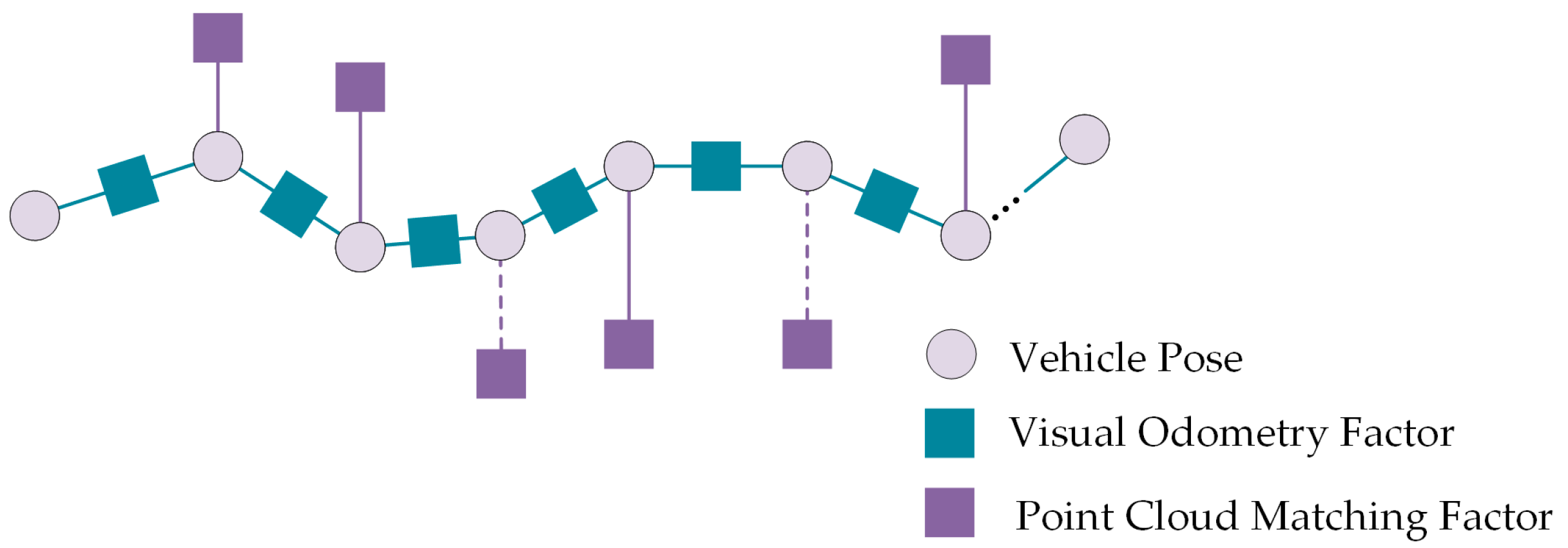
5.4. Localization Based on Pose Graph Optimization

With visual odometry, a typical dead-reckoning method, the accumulated error will lead to a drift in the localization result with increased vehicle travel distance. The global localization results matching with prior VPCM can overcome pose drift and recover the vehicle pose in the case of tracking loss. However, mismatches may lead to catastrophic localization errors.

We designed a localization algorithm based on global pose graph optimization, which integrates the dead-reckoning results of the odometry with the geometric matching result from prior VPCM. This approach effectively leverages the short-term accuracy of odometry and the global constraints of the prior map. The joint optimization factors only include the outputs of the odometry and geometric matching localization results, which maintains the moderate optimization size, thereby reducing the overall computational complexity. Furthermore, joint optimization can effectively suppress the drift error of odometry. The optimized poses further provide reliable pose estimates for point cloud matching, which enhances the overall robustness of the system and reduces the impact of mismatch.

The visual odometry calculates the pose increment and outputs the vehicle pose at each moment starting from the initial frame. We transform the local point cloud based on the optimized pose and match it with the prior map. If the matching succeeds, the global pose graph provides the fusion localization result. If it fails, the vehicle pose is calculated based on the historical localization and the real-time increment output by odometry. We construct the global pose graph shown in Figure 7, where the vehicle pose at every frame serves as an individual node. The successful matching and localization results at irregular intervals provide global constraints for the visual odometry, as shown by the solid line connection factor. Similar to the loop closure correction in the classic SLAM system, this optimization framework distributes the drift error of odometry across the historical frames and performs batch adjustments, effectively maintaining the trajectory’s consistency.

Next, let’s introduce each constraint factor in detail.

• Visual Odometry Factor

The PMCL method assumes that visual odometry is accurate in the short term, which applies to most visual odometry algorithms. We use $T_{t_1}^g$ and $T_{t_2}^g$ to represent transformed poses of the vehicle in the geographical coordinate system at $t_1$ and $t_2$ time, respectively. The transformation between the two frames can be expressed as $T_{t_1}^{t_2}={(T_{t_2}^g)}^{-1}{T}_{t_1}^g$ and in Lie algebra form as ${\epsilon }_{t_1{t}_2}=In{[{(T_{t_2}^g)}^{-1}{T}_{t_1}^g]}^{\vee }$. Then, we add the left perturbation $\delta {\epsilon }_{t_1}$ and $\delta {\epsilon }_{t_2}$ to ${\epsilon }_{t_1}$ and ${\epsilon }_{t_2}$, and the error can be expressed as:

$$\begin{array}{ll}\stackrel{\wedge }{{\epsilon }_{t_1{t}_2}}& =In{\left[{\left(T_{t_2}^g\right)}^{-1}\exp \left({\left(-\delta {\epsilon }_{t_2}\right)}^{\wedge }\right)\exp \left({\left(\delta {\epsilon }_{t_1}\right)}^{\wedge }\right)T_{t_1}^g\right]}^{\vee }\\ & \approx {\epsilon }_{t_1{t}_2}-{\mathcal{J}}_r^{-1}\left({\epsilon }_{t_1{t}_2}\right)Ad\left({\left(T_{t_1}^g\right)}^{-1}\right)\delta {\epsilon }_{t_2}+{\mathcal{J}}_r^{-1}\left({\epsilon }_{t_1{t}_2}\right)Ad\left({\left(T_{t_1}^g\right)}^{-1}\right)\delta {\epsilon }_{t_1}\end{array}$$

(12)

where ${\mathcal{J}}_r^{-1}\left(\epsilon \right)\approx I+{\displaystyle \frac{1}{2}}\left[\begin{array}{cc}{\varphi }_{\epsilon }^{\wedge }& {\rho }_{\epsilon }^{\wedge }\\ 0& {\varphi }_{\epsilon }^{\wedge }\end{array}\right]$, and $Ad\left(T\right)=\left[\begin{array}{cc}R& t^{\wedge }R\\ 0& R\end{array}\right]$.

2.

VPCM Matching Localization Factor

Assume that the latest vehicle pose, calculated based on the optimized historical trajectory and real-time increments from the odometry, is $T_{\psi }$. The matching localization result of the transformed local point cloud with the prior VPCM is $T_{\Delta }$. They should be the same, with the error as $e_{\psi }=In{(T_{\psi }^{-1}{T}_{\Delta })}^{\vee }$.

On this basis, we add the left perturbation $\phi$ to $T_{\psi }$.

$$\begin{array}{lll}{\stackrel{\wedge }{e}}_{\psi }& =In{\left(T_{\psi }^{-1}\exp \left({\left(-\phi \right)}^{\wedge }\right)T_{\Delta }\right)}^{\vee }& =In{\left(T_{\psi }^{-1}{T}_{\Delta }\exp \left({\left(-T_{\Delta }^{-1}\phi \right)}^{\wedge }\right)\right)}^{\vee }\\ & =In{\left(T_{\psi }^{-1}{T}_{\Delta }\left[I-{\left(T_{\Delta }^{-1}\phi \right)}^{\wedge }\right]\right)}^{\vee }& \approx e_{\psi }-{\mathcal{J}}^{-1}\left(e_{\psi }\right)Ad\left(T_{\Delta }^{-1}\right)\phi \end{array}$$

(13)

The Jacobian matrix of $T_{\psi }$ is shown in Equation (14).

$${\displaystyle \frac{\partial e_{\psi }}{\partial \phi }}=-{\mathcal{J}}^{-1}\left(e_{\psi }\right)Ad\left(T_{\Delta }^{-1}\right)$$

(14)

The optimization process of the global pose graph is adjusts the nodes to match all edges maximally. Compared to traditional filtering algorithms, the main advantage of pose graph optimization is incorporating historical information, often achieving a higher accuracy level. However, as the vehicle travel distance increases, the expanding optimization scale will impact the real-time performance of the localization system. We design a sliding window method to throw historical data from much earlier periods when the computation complexity exceeds real-time capability, and keep the window in a limited size.

6. Experiment Results

This paper experiments on the campus-collected and KITTI public datasets to evaluate the algorithms’ performance in real-world scenarios. We used the Zed2 stereo camera to capture visual images in the campus experiment, and the NovAtel OEM7 RTK device provided ground truth location information. The experimental vehicle is shown in Figure 8. We have $K_{iter}=10,{\tau }_{\max }=1m,{\tau }_{\min }=0.4m,N_{thre}=50$.

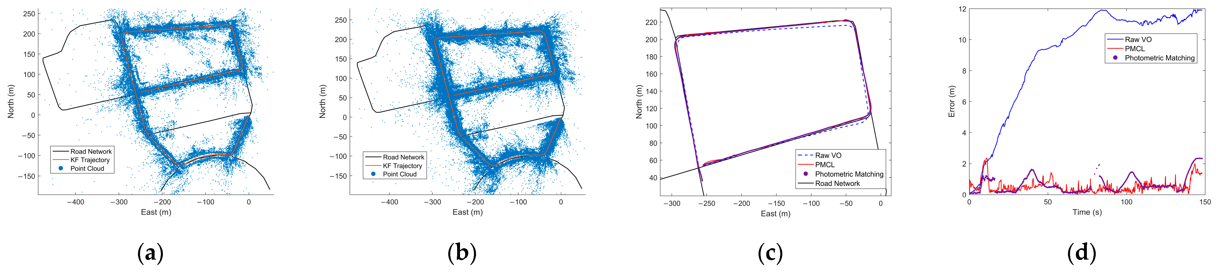
6.1. Map Construction Experiment on KITTI

To test the effectiveness and accuracy of the SAMC method designed in this paper, we first compare it with the keyframe-based classic open-source ORB-SLAM2 algorithm [43] and the map construction method in [39] on the KITTI dataset. Using Sequence 08 as the example, which features the long path length and wide coverage, the map construction effect of ORB-SLAM2 on the regional road network is shown in Figure 9a. ORB-SLAM2 can construct the VPCM, but this method relies on dead reckoning. The drift error can be suppressed in scenarios with loop closures, but it cannot be fundamentally eliminated due to the absence of absolute external constraints. Due to this, the constructed keyframe trajectory and point cloud distribution deviate from the road area, as shown in the enlarged area of Figure 9a. The authors of [39] introduce satellite references after constructing the visual map, achieving overall correction of keyframe trajectories and point clouds, as shown in Figure 9b. However, conflicts in correction coefficients between covisible keyframes will introduce new map errors, and we will provide a quantitative comparison in

Table 1. The map construction of different methods on the KITTI dataset.

	Number of KFs		Number of MPs		Matching Number		Map Size (M)		Error (m)
	[43]	SAMC	[43]	SAMC	[43]	SAMC	[43]	SAMC	[43]	[39]	SAMC
00	1418	4541	132,700	500,172	365.6	551.0	177.062	5.724	6.74	0.11	0.003
02	1740	4661	176,842	607,682	303.9	484.6	217.357	7.079	13.92	0.13	0.015
03	227	801	25,510	87,263	372.2	606.3	28.437	1.02	1.34	0.20	0.006
04	155	271	16,179	34,444	326.0	442.6	19.431	0.3935	0.71	0.23	0.006
05	724	2761	71,765	296,154	338.4	545.9	90.539	3.463	1.95	0.10	0.002
06	507	1101	39,980	123,572	344.6	447.0	63.456	1.444	1.64	0.12	0.002
07	255	1101	26,768	112,672	353.7	620.8	31.847	1.319	0.78	0.09	0.007
08	1203	4071	115,245	451,053	296.4	515.2	150.165	5.271	11.61	0.17	0.002
09	588	1591	56,668	196,518	293.4	473.0	73.374	2.291	5.60	0.11	0.002
10	328	1201	30,827	131,501	289.1	512.9	40.896	1.537	3.65	0.10	0.006

. The SAMC method introduces constraints from global NRTK, constructing the map optimization algorithm based on the enforced constraints of inverse external parameters, which integrates the high-precision positioning information of NRTK strongly with the reprojection errors of map points, i.e., the spatial accuracy of map points, thereby enhancing the accuracy of the prior point cloud. The map construction effect is shown in Figure 9c.

Additionally, we comprehensively compare the SAMC method with ORB-SLAM2 and the method in [39] on the KITTI dataset, and the primary comparison metrics are shown in Table 1. In addition to accuracy, our method uses the NRTK data to track image frames during the mapping process, which helps generate more map points and inter-frame matching points, providing more information support for matching and localization. Compared to ORB-SLAM2, our method demonstrates higher data extraction efficiency, with increases in the number of extracted keyframes, map points, and average inter-frame matching points by 209.3%, 266.9%, and 58.4%, respectively. In terms of map storage size, our method effectively reduces space requirements as it does not need to store the descriptor data required for photometric localization. The storage capacity is only 3.3% of that required by ORB-SLAM2. The method in [39] is similar to ORB-SLAM2 in terms of extraction efficiency and required storage space, so these details are not repeated here. On the other hand, our method tightly integrates NRTK data during the mapping process rather than performing overall correction after map construction completion like [39], achieving a centimeter-level map construction accuracy. It is important to note that the map accuracy mentioned here primarily focuses on the precision of keyframe trajectories and does not consider the accuracy of map points. The accuracy of map points cannot be evaluated using specific metrics and will be assessed in the subsequent localization experiments.

6.2. Localization Experiment on KITTI

We conducted the localization experiments using the prior VPCM constructed in Section 6.1. The front-end odometry in Section 5.1 provides the real-time local point cloud for matching, including the real-time keyframe pose and the map points it can observe. The features in the prior map exhibit invariance, and the camera perspectives during localization are the same as those in the mapping process, providing optimal data support for matching to validate the effectiveness and accuracy of the proposed localization method. During the localization experiments, we ban the loop closure optimization function to validate the performance of the localization algorithm better.

We first compare the localization performance of the PMCL method with the original odometry on KITTI sequences 00, 02, 05, and 08, which have long path lengths, wide coverage, and are prone to drift error in odometry localization. The experiment results are shown in Figure 10 and Figure 11. All subgraphs in Figure 10 show the localization trajectory on the road network map, indicating that the PMCL method has a good trajectory correction effect. All subgraphs in Figure 11 display the trend of localization error over time. With increasing traveling distance, the original visual odometry error gradually increases. The PMCL method effectively suppresses the drift error, reducing the average localization error from 11.6 m to centimeter-level.

Then, we compare our localization method with the localization mode of ORB-SLAM2 and other map-based algorithms, including [31,32,33,34,35,38,39,41]. The average localization errors (m) of different methods are shown in

Table 2. The localization performance of different methods.

Seq	[43]	[31]	[32]	[33]	[34]	[35]	[38]	[39]	[41]	PMCL
00	6.8096	0.146	0.5796	0.1325	0.5765	5.1	0.3367	0.1547	1.27	0.1233
02	13.819	0.045	5.9826	0.2205	—	10.2	0.3596	0.206	—	0.2123
03	1.3971	0.032	—	0.2368	—	—	0.3869	0.2767	—	0.0963
04	0.6716	0.027	0.2837	0.4496	—	—	—	0.2512	—	0.0791
05	1.8757	0.044	0.7450	0.1462	0.4783	—	0.2498	0.1416	3.18	0.1176
06	1.6533	0.033	0.7481	0.3753	0.7412	6.8	0.1956	0.1528	—	0.0669
07	0.7387	0.042	0.1789	0.1305	0.6630	3.6	0.3392	0.1401	—	0.0738
08	11.374	0.056	1.5473	0.1440	1.2784	—	1.9745	0.2655	—	0.1304
09	5.7846	0.035	0.9876	0.1799	0.7168	11.4	0.4773	0.1773	1.94	0.1503
10	4.2495	0.027	0.6663	0.2398	0.5023	—	0.3749	0.1597	—	0.0954
Error/Frame	7.4686	0.0645	1.9880	0.1838	0.7596	7.7175	0.6432	0.1910	—	0.1363

. ORB-SLAM2 [43] proposes a localization mode based on the bag-of-words model and feature corner optical descriptors. The method in [31] is a typical LiDAR-based method, which locates the vehicle by matching the real-time LiDAR scan with the EQT map. The authors of [32] use the local 3D map generated from LiDAR SLAM to match the 2D map. The methods in [33,34,35] are all LiDAR-camera-fused methods. The authors of [33] utilize stereo cameras to generate disparity maps and estimate the vehicle pose by minimizing depth residuals. The authors of [34] propose a decoupling optimization strategy to compute the affine transformation for the monocular scale ambiguity to align the point clouds from vision and LiDAR map. The authors of [35] associate the local semantic object map with a LiDAR reference map to achieve localization. The authors of [38] tightly couple the semantic and structure information of prior maps. The camera poses, and data associations are jointly optimized for accurate localization. The Visual SLAM algorithm and real trajectory data are used to construct a global photometric feature map [39], enabling camera localization in geographic coordinates. The authors of [41] utilize the SGBM algorithm to generate the real-time visual point cloud and achieve accurate matching localization through NDT transformation with a pre-built visual point cloud map. However, the generation process of the prior visual point cloud map relies on LiDAR assistance.

The localization accuracy of ORB-SLAM2 is constrained by drift errors inherent in the original map. While achieving sub-meter precision in short-distance or well-constrained loop closure scenarios such as KITTI sequences 04 and 07, it exhibits significant error drift in other sequences with large-scale environments or sparse features. In contrast, the SAMC method proposes the theory of enforced constraints of inverse external parameters, introducing the external global drift-free constraints of NRTK to construct the high-precision map. The corresponding PMCL method achieves centimeter-level localization accuracy on the KITTI dataset, effectively reducing the original odometry drift error. We bold the best overall and the best camera-based methods separately. Our method demonstrates a significant localization accuracy advantage compared to similar map-based algorithms, second only to the LiDAR-based scan match localization method [31]. The methods in [35,38] utilize deep learning techniques to identify semantic information in the environment, which can accelerate matching speed and enhance robustness. The PMCL method preloads sub-maps through iterative internal road segments of the road network, which can also accelerate matching and reduce mismatches. Additionally, compared to other types of maps, the topological road network has stronger robustness and long-term stability. Even if the environment around the road changes, causing other semantic information loss, the structure of the road itself will not change. The methods in [33,34,41] are most similar to the PMCL method, achieving localization through deep residuals or point cloud matching. However, the prior maps in these methods rely on LiDAR-assisted construction, whereas our maps are built using cameras. Compared to the most similar method [33], the proposed approach reduced the average per-frame localization error by 25.84%. The main reason for this improvement is that we incorporate the regional road network and reference keyframes in the map construction process. When there are insufficient matching point pairs, the PMCL method transforms the real-time pose and corresponding local point cloud to the nearest map reference keyframe pose. This design capitalizes on the advantage of NRTK, utilizing the high-precision prior reference keyframe trajectory constructed under its assistance to provide a better initial value reference and help match a greater number of point pairs, which is very suitable for vehicle navigation systems that exhibit stability in pitch and roll. The method in [39] does not rely on LiDAR for map construction and localization, which is similar to our approach. Its localization precision is comparable to the most accurate method [33], only inferior to pure LiDAR solutions [31]. However, it relies on photometric matching [16], which has a clear advantage on the KITTI dataset. Subsequent experiments will compare our method against its performance using more challenging real-world datasets.

6.3. Localization Experiment in Different Scenarios

The experiments on the KITTI dataset demonstrate the effectiveness and accuracy of the proposed method. In practical application scenarios, it is hard to provide the same level of data support as the KITTI dataset localization experiments. This is primarily due to three reasons: (1) The camera perspectives during mapping and localization processes are inconsistent. (2) There are variations in light and dynamic objects between different periods of the same day. (3) There are differences in the primary environment between different seasons, leading to inconsistencies in the extracted features during the mapping and localization processes. This paper utilizes real-world collected campus data to validate the localization performance of our method under the influence of the aforementioned adverse factors. The collected campus dataset is shown in

Table 3. The real-world campus dataset.

Map-Seq	Collection Time	Distance (m)	Loc-Seq
Campus-01	2024-04-16 10:52:20	1588.54	Campus-02
Campus-02	2024-07-17 11:01:27	1195.44	——
Campus-03	2024-07-17 11:24:16	1296.72	Campus-05
Campus-04	2024-07-17 16:38:58	1194.71	Campus-05
Campus-05	2024-07-17 16:44:45	776.475	——

, where Map-Seq and Loc-Seq denote the sequences used for map construction and localization, respectively. The range of Map-Seq can cover the corresponding Loc-Seq. For instance, the first row indicates that sequence Campus-01 is the VPCM construction set, and sequence Campus-02 is used for localization performance testing. These diverse experiment combinations can assess the performance of the proposed method under various interference scenarios.

1.

E1: Impact of the camera perspective difference

This experiment primarily validates the localization performance of our method in the approximately constant environment, where the construction of prior VPCM and matching localization are conducted within a limited timeframe. This experiment has no significant changes in lighting and environment, with only minor variations in dynamic objects. We mainly focus on the impact of camera perspective differences during the mapping and localization processes. In this experiment, we use the dataset Campus-04 to construct the prior VPCM, and the localization dataset Campus-05 is collected shortly after Campus-04.

2.

E2: Impact of lighting changes at different time of the day

In this experiment, the construction of prior VPCM and matching localization are conducted at different times of the day, with no significant changes in the primary environment, only differences in lighting and dynamic objects. The purpose is to verify the impact of lighting changes during the mapping and localization processes. We use the dataset Campus-03 to construct the prior VPCM, and the localization dataset Campus-05 is collected more than five hours after Campus-03, with lighting changes.

3.

E3: Impact of environmental changes

In this experiment, the construction of prior VPCM and matching localization are conducted in two different seasons, with significant changes in the primary environment and drastically different dynamic objects. The purpose is to verify the impact of environmental changes during the mapping and localization processes. We use the dataset Campus-01 to construct the prior VPCM, and the localization dataset Campus-02 is collected over three months after Campus-01, with seasonal environmental changes and a section of road where renovations of surrounding buildings caused fundamental environmental changes.

We compare the proposed method with the similarly camera-based method in [39], which also uses satellite references to correct map errors during the mapping phase. The authors of [39] construct the photometric feature map and rely on photometric matching algorithms for localization [16]. This method demonstrates outstanding performance in localization experiments on the KITTI dataset. The map construction effects of the method in [39] and the SAMC method are shown in subfigures (a) and (b) of Figure 12, Figure 13 and Figure 14, respectively. Both methods can effectively suppress the accumulated error of keyframe trajectories by introducing satellite references and correct the point clouds to the road range. Furthermore, our method constructs a higher-density visual point cloud, which can provide more support for localization data.

All subfigures (c) and (d) in Figure 12, Figure 13 and Figure 14 show the localization trajectories and error curves over time of the original odometry, the photometric matching method in [39], and the PMCL method. It can be seen that the PMCL method can effectively correct the localization trajectory to the range of the road point cloud. The photometric matching method also achieves effective localization. However, its performance gradually declines due to variations in lighting and environment between the map construction and localization phases. As shown in

Table 4. The localization performance of different methods on real-world datasets.

	Matching Success Rate		Matching Point Average Error (m)		Localization Average Error (m)
	[39]	PMCL	[39]	PMCL	RawVO	PMCL
E1	98.09%	99.67%	0.6639	0.4899	9.042	0.467
E2	87.16%	98.98%	0.9089	0.5295	9.042	0.531
E3	39.68%	60.83%	1.3437	0.5054	22.26	0.938

, in the E1 experiment, the localization performance of the photometric matching method is comparable to that of the PMCL method. While in the E2 experiment, the PMCL method demonstrates greater robustness to lighting changes compared to the photometric matching method. In the more challenging E3 experiment, the PMCL method improves the matching success rate by 21.15% and reduces the average matching localization error by 62.39% compared to the photometric matching method. Furthermore, the PMCL method consistently achieves high matching localization accuracy in the E1, E2, and E3 experiments, with an average error of approximately 0.5 m, indicating strong robustness to variations in camera perspective, lighting, and environmental conditions.

In the time period indicated by the red box in Figure 14c, the localization error of the PMCL method continuously increases. This is due to renovations of buildings around the road, which bring discrepancies between the prior VPCM and the actual environment landmark, leading to matching failures. Unlike the photometric matching method in [39], which cannot provide localization information during this phase, the PMCL method predicts the vehicle’s state based on the optimized historical trajectory and real-time odometry increments, while continuously matching the local point cloud with the VPCM. Although the localization error grows due to odometry incremental errors between adjacent frames, rapid correction can be achieved once successful matching occurs, as demonstrated by the quick reduction in error shown in Figure 14. The PMCL method utilizes the advantages of both odometry and map matching. Odometry can provide localization information in cases of matching failure and prior information for subsequent matching, while map matching results can, conversely, suppress odometry drift.

6.4. Time Performance

All experiments in this paper are conducted on a computer equipped with an Intel i7 2.3 GHz CPU and 16 GB of memory. The average time for the odometry to generate the real-time keyframe pose and the local point cloud is 0.051 s. The time for point cloud matching localization depends on the size of the real-time point cloud and sub-map reference, with an average time ranging from 0.008 to 0.017 s. All data processing can be completed within the image capture cycle, which meets the time requirements for localization.

7. Discussion

To evaluate the map construction and matching localization performance of the proposed method, we conduct experiments on the public and real-world datasets. In the map construction experiments, as shown in Figure 9, Figure 12, Figure 13 and Figure 14, the VPCM constructed by the SAMC method is corrected to the road areas and has a higher density compared to the methods in [39,43]. Table 1 demonstrates that the SAMC method achieves higher data extraction efficiency and accuracy, and requires less storage space. In the localization experiments, Figure 10, Figure 11, Figure 12, Figure 13 and Figure 14 indicate that the PMCL method effectively corrects the localization trajectory to the road areas and suppresses the cumulative drift. Table 2 shows that the PMCL method surpasses most map-based methods in accuracy. On more challenging real-world datasets, compared to the similar camera-based method in [39], the PMCL method demonstrates higher matching success rates and localization accuracy, as shown in Table 4.

Overall, this paper proposes a visual point cloud map construction and matching localization method that demonstrates advantages over similar approaches. However, there are still aspects that can be further improved:

(1)

The evaluation of map accuracy primarily focuses on the precision of keyframes and the overall consistency of map points covering the roads. The precision of individual map points cannot be determined, making it difficult to discern whether localization errors primarily arise from potential errors in maps or from the matching method. In future work, the high-precision LiDAR can be introduced to assess the deviation levels of map points, further analyze the respective impacts of potential errors in maps and the matching method on localization accuracy.

(2)

In the real-world experiment E3, environmental changes resulted in sustained matching failures over a period of time, making it impossible to introduce real-time constraints. In extreme cases, when significant environmental changes occur and the map is not updated, the localization error may continuously diverge. Future work could consider integrating road-network-maps-assisted localization algorithms, enabling localization under multi-map joint constraints.

(3)

The VPCM constructed in this paper is situated in the ENU geographic coordinate system commonly used for vehicle localization. Within a regional range, the geographic coordinate system approximates a fixed geographic reference. However, the east and north directions can produce biases due to Earth’s curvature when applied to large cities. Future work could optimize the map model and global construction methods to enhance scalability to large city-scale maps.

8. Conclusions

This paper proposes a visual point cloud map construction and matching localization method for autonomous vehicles. We design a new visual point cloud map model that incorporates the regional road network base. This design can effectively partition the spatial point cloud, enhancing data indexing speed during the matching and localization. Then, we propose the SAMC method based on the multi-sensors fusion, enabling the balance of different error terms and the autonomous construction of the geographical high-precision prior VPCM. By introducing geometric constraints from the prior map, the PMCL method continuously corrects odometry errors. Simultaneously, the fusion localization results significantly enhance the success rate and accuracy of geometric matching. The method proposed in this paper is a pure visual solution that encompasses both autonomous map construction and robust localization with low data dependency, leading to lower construction costs, storage space requirements, and computational costs. The experiment results on the public and campus datasets show that our method can integrate information from multiple sensors and autonomously construct high-precision VPCM references. Compared to the base method, the SAMC method doubles the data extraction efficiency and reduces the storage space requirement for localization data to 3.3%. In situations where satellite signals are unavailable, the introduced constraints from the prior map can effectively suppress odometry localization drift error. The PMCL method reduces the average error per frame by 25.84% compared to the similar methods on the KITTI dataset. Additionally, in more challenging real-world datasets, the PMCL method improves the matching success rate by 21.15% and reduces the average localization error by 62.39% compared to the similar camera-based method, demonstrating robustness against lighting and environment changes in vehicle traveling.

Overall, the proposed method leverages the pre-constructed high-precision map to achieve accurate vehicle localization in GNSS-denied environments, thereby enhancing its role as the anchor points in co-operative navigation systems with drones. Additionally, the proposed visual point cloud map can be extended to low-altitude drone navigation scenarios in future work.

References

1. Wang, N.; Li, X.; Suo, Z.; Fan, J.; Wang, J.; Xie, D. Traversability Analysis and Path Planning for Autonomous Wheeled Vehicles on Rigid Terrains. Drones 2024, 8, 419. [Google Scholar] [CrossRef]
2. Bai, S.; Lai, J.; Lyu, P.; Cen, Y.; Sun, X.; Wang, B. Performance enhancement of tightly coupled GNSS/IMU integration based on factor graph with robust TDCP loop closure. IEEE Trans. Intell. Transp. Syst. 2023, 25, 2437–2449. [Google Scholar] [CrossRef]
3. Lu, Y.; Ma, H.; Smart, E.; Yu, H. Real-time performance-focused localization techniques for autonomous vehicle: A review. IEEE Trans. Intell. Transp. Syst. 2021, 23, 6082–6100. [Google Scholar] [CrossRef]
4. Liu, C.; Zhao, J.; Sun, N. A review of collaborative air-ground robots research. J. Intell. Robot. Syst. 2022, 106, 60. [Google Scholar] [CrossRef]
5. Renner, A.; Supic, L.; Danielescu, A.; Indiveri, G.; Frady, E.P.; Sommer, F.T.; Sandamirskaya, Y. Visual odometry with neuromorphic resonator networks. Nat. Mach. Intell. 2024, 6, 653–663. [Google Scholar] [CrossRef]
6. Wang, G.; Wu, X.; Jiang, S.; Liu, Z.; Wang, H. Efficient 3d deep lidar odometry. IEEE Trans. Pattern Anal. Mach. Intell. 2022, 45, 5749–5765. [Google Scholar] [CrossRef] [PubMed]
7. Lyu, Y.; Hua, L.; Wu, J.; Liang, X.; Zhao, C. Robust Radar Inertial Odometry in Dynamic 3D Environments. Drones 2024, 8, 197. [Google Scholar] [CrossRef]
8. Wei, J.; Deng, H.; Wang, J.; Zhang, L. AFO-SLAM: An improved visual SLAM in dynamic scenes using acceleration of feature extraction and object detection. Meas. Sci. Technol. 2024, 35, 116304. [Google Scholar] [CrossRef]
9. Jung, J.H.; Cha, J.; Chung, J.Y.; Kim, T.I.; Seo, M.H.; Park, S.Y.; Yeo, J.Y.; Park, C.G. Monocular visual-inertial-wheel odometry using low-grade IMU in urban areas. IEEE Trans. Intell. Transp. Syst. 2020, 23, 925–938. [Google Scholar] [CrossRef]
10. You, Z.; Liu, L.; Bethel, B.J.; Dong, C. Feature comparison of two mesoscale eddy datasets based on satellite altimeter data. Remote Sens. 2021, 14, 116. [Google Scholar] [CrossRef]
11. Cheng, H.M.; Song, D. Graph-based proprioceptive localization using a discrete heading-length feature sequence matching approach. IEEE Trans. Robot. 2021, 37, 1268–1281. [Google Scholar] [CrossRef]
12. Shi, Y.; Li, H. Beyond cross-view image retrieval: Highly accurate vehicle localization using satellite image. In Proceedings of the 2022 IEEE/CVF Conference on Computer Vision and Pattern Recognition, New Orleans, LA, USA, 18–24 June 2022; pp. 17010–17020. [Google Scholar]
13. Cai, Y.; Lu, Z.; Wang, H.; Chen, L.; Li, Y. A lightweight feature map creation method for intelligent vehicle localization in urban road environments. IEEE Trans. Instrum. Meas. 2022, 71, 1–15. [Google Scholar] [CrossRef]
14. Li, J.; Qin, H.; Wang, J.; Li, J. Openstreetmap-based autonomous navigation for the four wheel-legged robot via 3d-lidar and ccd camera. IEEE Trans. Ind. Electron. 2021, 69, 2708–2717. [Google Scholar] [CrossRef]
15. Guo, S.; Rong, Z.; Wang, S.; Wu, Y. A LiDAR SLAM with PCA-based feature extraction and two-stage matching. IEEE Trans. Instrum. Meas. 2022, 71, 1–11. [Google Scholar] [CrossRef]
16. Campos, C.; Elvira, R.; Rodríguez, J.J.G.; Montiel, J.M.; Tardós, J.D. Orb-slam3: An accurate open-source library for visual, visual–inertial, and multimap slam. IEEE Trans. Robot. 2021, 37, 1874–1890. [Google Scholar] [CrossRef]
17. Gupta, A.; Fernando, X. Simultaneous localization and mapping (slam) and data fusion in unmanned aerial vehicles: Recent advances and challenges. Drones 2022, 6, 85. [Google Scholar] [CrossRef]
18. Elaksher, A.; Ali, T.; Alharthy, A. A quantitative assessment of LiDAR data accuracy. Remote Sens. 2023, 15, 442. [Google Scholar] [CrossRef]
19. Im, J.H.; Im, S.H.; Jee, G.I. Vertical corner feature based precise vehicle localization using 3D LIDAR in urban area. Sensors 2016, 16, 1268. [Google Scholar] [CrossRef] [PubMed]
20. Li, X.; Shen, Y.; Lu, J.; Jiang, Q.; Xie, O.; Yang, Y.; Zhu, Q. DyStSLAM: An efficient stereo vision SLAM system in dynamic environment. Meas. Sci. Technol. 2022, 34, 025105. [Google Scholar] [CrossRef]
21. Yabuuchi, K.; Wong, D.R.; Ishita, T.; Kitsukawa, Y.; Kato, S. Visual localization for autonomous driving using pre-built point cloud maps. In Proceedings of the 2021 IEEE Intelligent Vehicles Symposium, Nagoya, Japan, 11–17 July 2021; pp. 913–919. [Google Scholar]
22. Zhou, G.; Yuan, H.; Zhu, S.; Huang, Z.; Fan, Y.; Zhong, X.; Du, R.; Gu, J. Visual Localization in a Prior 3D LiDAR Map Combining Points and Lines. In Proceedings of the 2021 IEEE International Conference on Robotics and Biomimetics (ROBIO), Sanya, China, 6–10 December 2021; pp. 1198–1203. [Google Scholar]
23. Dhoke, A.; Shankar, P. Exploring the Complexities of GPS Navigation: Addressing Challenges and Solutions in the Functionality of Google Maps. In Proceedings of the 2023 7th International Conference On Computing, Communication, Control And Automation (ICCUBEA), Pune, Maharashtra, India, 18–19 August 2023; pp. 1–6. [Google Scholar]
24. Grinberger, A.Y.; Minghini, M.; Juhász, L.; Yeboah, G.; Mooney, P. OSM Science—The Academic Study of the OpenStreetMap Project, Data, Contributors, Community, and Applications. ISPRS Int. J. Geo-Inf. 2022, 11, 230. [Google Scholar] [CrossRef]
25. Sun, H.; Xu, Z.; Yao, L.; Zhong, R.; Du, L.; Wu, H. Tunnel monitoring and measuring system using mobile laser scanning: Design and deployment. Remote Sens. 2020, 12, 730. [Google Scholar] [CrossRef]
26. Chalvatzaras, A.; Pratikakis, I.; Amanatiadis, A.A. A survey on map-based localization techniques for autonomous vehicles. IEEE Trans. Intell. Veh. 2022, 8, 1574–1596. [Google Scholar] [CrossRef]
27. Li, S.; Liu, S.; Zhao, Q.; Xia, Q. Quantized self-supervised local feature for real-time robot indirect VSLAM. IEEE ASME Trans. Mechatron. 2021, 27, 1414–1424. [Google Scholar] [CrossRef]
28. Mo, J.; Islam, M.J.; Sattar, J. Fast direct stereo visual SLAM. IEEE Robot. Autom. Lett. 2021, 7, 778–785. [Google Scholar] [CrossRef]
29. Daoud, H.A.; Md. Sabri, A.Q.; Loo, C.K.; Mansoor, A.M. SLAMM: Visual monocular SLAM with continuous mapping using multiple maps. PLoS ONE 2018, 13, e0195878. [Google Scholar] [CrossRef] [PubMed]
30. Elvira, R.; Tardós, J.D.; Montiel, J.M. ORBSLAM-Atlas: A robust and accurate multi-map system. In Proceedings of the 2019 IEEE/RSJ International Conference on Intelligent Robots and Systems (IROS), Macau, China, 4–8 November 2019; pp. 6253–6259. [Google Scholar]
31. Wen, J.; Tang, J.; Liu, H.; Qian, C.; Fan, X. Real-time scan-to-map matching localization system based on lightweight pre-built occupancy high-definition map. Remote Sens. 2023, 15, 595. [Google Scholar] [CrossRef]
32. Lee, S.; Ryu, J.H. Autonomous vehicle localization without prior high-definition map. IEEE Trans. Robot. 2024, 40, 2888–2906. [Google Scholar] [CrossRef]
33. Kim, Y.; Jeong, J.; Kim, A. Stereo camera localization in 3d lidar maps. In Proceedings of the 2018 IEEE/RSJ International Conference on Intelligent Robots and Systems (IROS), Madrid, Spain, 1–5 October 2018; pp. 1–9. [Google Scholar]
34. Zhang, C.; Zhao, H.; Wang, C.; Tang, X.; Yang, M. Cross-modal monocular localization in prior lidar maps utilizing semantic consistency. In Proceedings of the 2023 IEEE International Conference on Robotics and Automation (ICRA), London, UK, 29 May–2 June 2023; pp. 4004–4010. [Google Scholar]
35. Ankenbauer, J.; Lusk, P.C.; Thomas, A.; How, J.P. Global localization in unstructured environments using semantic object maps built from various viewpoints. In Proceedings of the 2023 IEEE/RSJ international conference on intelligent robots and systems (IROS), Detroit, MI, USA, 1–5 October 2023; pp. 1358–1365. [Google Scholar]
36. Wang, Z.; Zhang, Z.; Kang, X. A Visual Odometry System for Autonomous Vehicles Based on Squared Planar Markers Map. In Proceedings of the 2023 IEEE International Conference on Unmanned Systems (ICUS), Hefei, China, 13–15 October 2023; pp. 311–316. [Google Scholar]
37. Qin, T.; Li, P.; Shen, S. Relocalization, global optimization and map merging for monocular visual-inertial SLAM. In Proceedings of the 2018 IEEE International Conference on Robotics and Automation (ICRA), Brisbane, Australia, 21–25 May 2018; pp. 1197–1204. [Google Scholar]
38. Liang, S.; Zhang, Y.; Tian, R.; Zhu, D.; Yang, L.; Cao, Z. Semloc: Accurate and robust visual localization with semantic and structural constraints from prior maps. In Proceedings of the 2022 International Conference on Robotics and Automation (ICRA), Philadelphia, PA, USA, 23–27 May 2022; pp. 4135–4141. [Google Scholar]
39. Kascha, M.; Xin, K.; Zou, X.; Sturm, A.; Henze, R.; Heister, L.; Oezberk, S. Monocular Camera Localization for Automated Driving. In Proceedings of the 2023 29th International Conference on Mechatronics and Machine Vision in Practice (M2VIP), Queenstown, New Zealand, 15–17 November 2023; pp. 1–6. [Google Scholar]
40. Churchill, W.; Newman, P. Experience-based navigation for long-term localisation. Int. J. Robot. Res. 2013, 32, 1645–1661. [Google Scholar] [CrossRef]
41. Lin, X.; Wang, F.; Yang, B.; Zhang, W. Autonomous vehicle localization with prior visual point cloud map constraints in GNSS-challenged environments. Remote Sens. 2021, 13, 506. [Google Scholar] [CrossRef]
42. Elsayed, H.; El-Mowafy, A.; Wang, K. Bounding of correlated double-differenced GNSS observation errors using NRTK for precise positioning of autonomous vehicles. Measurement 2023, 206, 112303. [Google Scholar] [CrossRef]
43. Mur-Artal, R.; Tardós, J.D. Orb-slam2: An open-source slam system for monocular, stereo, and rgb-d cameras. IEEE Trans. Robot. 2017, 33, 1255–1262. [Google Scholar] [CrossRef]
44. Xu, S.; Sun, Y.; Zhao, K.; Fu, X.; Wang, S. Road-network-map-assisted vehicle positioning based on pose graph optimization. Sensors 2023, 23, 7581. [Google Scholar] [CrossRef] [PubMed]
45. Leutenegger, S.; Lynen, S.; Bosse, M.; Siegwart, R.; Furgale, P. Keyframe-based visual–inertial odometry using nonlinear optimization. Int. J. Robot. Res. 2015, 34, 314–334. [Google Scholar] [CrossRef]
46. Qin, T.; Li, P.; Shen, S. Vins-mono: A robust and versatile monocular visual-inertial state estimator. IEEE Trans. Robot. 2018, 34, 1004–1020. [Google Scholar] [CrossRef]
Figure 1. The overall system framework: dashed arrows are executed once, solid arrows are executed periodically, grey blocks are the input, blue blocks are the constants, green blocks are the intermediate variables, yellow blocks are the execution modules, and the orange block is the output.
Drones 09 00511 g001
Figure 2. The tracking process under the NRTK assistance. The reprojection error is the error between the map point’s matching point and the projection point in the same image frame.
Drones 09 00511 g002
Figure 3. Global optimization factor graph of the point cloud map construction. The reprojection errors and absolute position errors are correlated through the enforced constraints of inverse external parameters.
Drones 09 00511 g003
Figure 4. The road segment to which the keyframes belong is determined based on its geographic location. The keyframes located at the intersections of the roads usually belong to multiple RNBEs, as shown in the enlarged view in (b).
Drones 09 00511 g004
Figure 5. The graphic flowchart of the localization process. Grey blocks are the input, green blocks are the intermediate variable, yellow blocks are the execution modules, the purple diamond-shaped box is the decision module, and the orange block is the output.
Drones 09 00511 g005
Figure 6. Iterative Strategy of the belonging RNBE. The iteration process primarily depends on changes in the vehicle’s heading and travel distance, but in complex road network structures, it relies on subsequent accurate geometric matching localization results.
Drones 09 00511 g006
Figure 7. Global pose graph optimization for localization: dashed lines indicate the matching failure.
Drones 09 00511 g007
Figure 8. Experimental vehicle for the campus dataset: (a) shows the onboard experimental platform, with the ZED2 stereo camera in the yellow box and the RTK device in the red box. (b) shows the actual installation effect of the vehicle-mounted experimental platform.
Drones 09 00511 g008
Figure 9. Mapping Effect of ORB-SLAM2, the method in [39], and the SAMC method on KITTI-08 Sequence. Compared to ORB-SLAM2, the latter two methods can suppress errors. (a) Mapping Effect of ORB-SLAM2. (b) Mapping Effect of method in [39]. (c) Mapping Effect of SAMC.
Drones 09 00511 g009
Figure 10. The localization trajectories of the original odometry and the PMCL method on the KITTI sequences 00, 02, 05, and 08.
Drones 09 00511 g010
Figure 11. The localization error curves over time of the original odometry and the PMCL method on the KITTI sequences 00, 02, 05, and 08.
Drones 09 00511 g011
Figure 12. Results of the real-world experiment E1. (a,b) show the mapping effect of the method in [39] and the SAMC method. (c,d) show the localization trajectories and error curves over time of the original odometry, the photometric matching method in [39], and the PMCL method.
Drones 09 00511 g012
Figure 13. Results of the real-world experiment E2. (a,b) show the mapping effect of the method in [39] and the SAMC method. (c,d) show the localization trajectories and error curves over time of the original odometry, the photometric matching method in [39], and the PMCL method.
Drones 09 00511 g013
Figure 14. Results of the real-world experiment E3. (a,b) show the mapping effect of the method in [39] and the SAMC method. (c,d) show the localization trajectories and error curves over time of the original odometry, the photometric matching method in [39], and the PMCL method.
Drones 09 00511 g014