Flight-Safe Inference: SVD-Compressed LSTM Acceleration for Real-Time UAV Engine Monitoring Using Custom FPGA Hardware Architecture

Abstract

Predictive maintenance (PdM) is a proactive strategy that enhances safety, minimizes unplanned downtime, and optimizes operational costs by forecasting equipment failures before they occur. This study presents a novel Field Programmable Gate Array (FPGA)-accelerated predictive maintenance framework for UAV engines using a Singular Value Decomposition (SVD)-optimized Long Short-Term Memory (LSTM) model. The model performs binary classification to predict the likelihood of imminent engine failure by processing normalized multi-sensor data, including temperature, pressure, and vibration measurements. To enable real-time deployment on resource-constrained UAV platforms, the LSTM’s weight matrices are compressed using Singular Value Decomposition (SVD), significantly reducing computational complexity while preserving predictive accuracy. The compressed model is executed on a Xilinx ZCU-104 FPGA and uses a pipelined, AXI-based hardware accelerator with efficient memory mapping and parallelized gate calculations tailored for low-power onboard systems. Unlike prior works, this study uniquely integrates a tailored SVD compression strategy with a custom hardware accelerator co-designed for real-time, flight-safe inference in UAV systems. Experimental results demonstrate a 98% classification accuracy, a 24% reduction in latency, and substantial FPGA resource savings—specifically, a 26% decrease in BRAM usage and a 37% reduction in DSP consumption—compared to the 32-bit floating-point SVD-compressed FPGA implementation, not CPU or GPU. These findings confirm the proposed system as an efficient and scalable solution for real-time UAV engine health monitoring, thereby enhancing in-flight safety through timely fault prediction and enabling autonomous engine monitoring without reliance on ground communication.

1. Introduction

In recent years, the aeronautical sector has made significant progress, ranging from UAV control systems using wearable sensors [1] to the adoption of advanced technologies for predictive maintenance in a context that requires exceptionally high standards of safety, reliability, and operational efficiency [2]. However, these tend to result in higher operational costs, unplanned downtime, and even safety risks owing to unexpected failures. Predictive Aircraft Maintenance (PdAM) provides a solution based on real-time information from state-of-the-art onboard sensors, flight data recorders, and diagnostic systems. Through data analytics, machine learning, or deep learning, PdAM predicts component faults before they occur, making possible condition-based maintenance, maximizing aircraft availability, minimizing unnecessary interventions, and enhancing safety margins [3]. Through real-time data analysis, PdAM identifies faults and estimates the sensor’s remaining useful life (RUL) threshold, performing maintenance only when required, thereby maximizing fleet efficiency and ensuring regulatory compliance [4]. Unmanned Aerial Vehicles (UAVs) become essential in several applications, including military surveillance, environmental monitoring, logistics, and disaster response. UAVs require high levels of dependability, safety, and real-time response due to their autonomous function in remote or hazardous environments. In contrast to manned aircraft, where pilots may frequently address initial indications of failure, UAVs depend exclusively on onboard systems to identify and react to abnormalities. Consequently, predictive maintenance (PdM) is essential for UAVs, as it anticipates component failures prior to their occurrence, thereby maintaining mission continuity, mitigating the risk of mid-air failures, and prolonging the operational lifespan of onboard equipment.

Singular Value Decomposition (SVD) is one of the central mathematical techniques employed for optimizing the deep learning (DL) models (for reducing the inference time) in predictive maintenance, namely its ability to lower dimensionality, eliminate noise, and identify anomalies in extensive sensor data [5] and robotic systems telemetries [6,7]. Although other compression methods exist, SVD was chosen for its potential to reveal hidden structures in complex aviation data. Nonetheless, its implementation must be validated by experimental comparisons with alternative methodologies to demonstrate its superiority when utilized alongside deep topologies such as LSTM networks. Singular Value Decomposition (SVD) improves prediction performance but encounters high computational costs. FPGAs address this issue through parallel processing, low latency, and power-efficient computation, making them suitable for speeding up SVD-optimized LSTM algorithms in real-time onboard applications [8]. This hardware-based solution provides faster data processing, real-time anomaly detection, and improved decision-making, eliminating the need for cumbersome cloud computing. It reduces maintenance costs, enhances flight safety, and optimizes aircraft management.

To substantiate the term ‘flight-safe,’ the proposed system emphasizes real-time operation, reduced inference latency, and deterministic control via FPGA acceleration, aligning with the responsiveness and reliability requirements critical to autonomous UAV missions.

Unlike prior works that separately explore SVD-based model compression or the FPGA acceleration of LSTM models, this study uniquely co-designs both SVD compression and a custom pipelined AXI-based FPGA hardware architecture optimized explicitly for UAV engine health monitoring. This integrated approach ensures real-time inference with minimal resource consumption, addressing the critical constraints of onboard UAV platforms. Moreover, the proposed method employs a tailored SVD compression strategy that balances accuracy and hardware efficiency, a gap not adequately addressed in previous research.

Although several studies have modeled RUL estimation as a regression problem to forecast the exact number of cycles before failure, our work adopts a classification-based approach. We predict whether a UAV engine is likely to fail within a specified number of cycles (e.g., 30), converting the RUL estimation problem into a binary classification task. This strategy simplifies deployment on low-power platforms, improves interpretability for fault-alert systems, and aligns better with actionable maintenance decisions. This formulation enables real-time failure warnings with minimal computational overhead, making it highly suitable for onboard UAV applications.

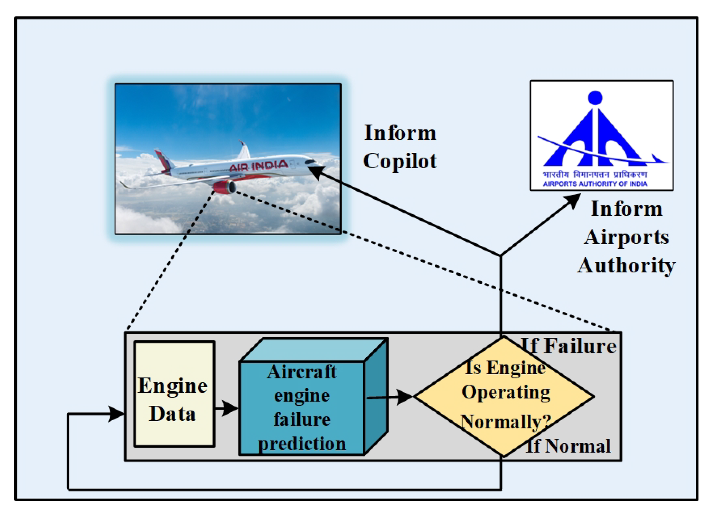
Figure 1 shows a real-time aircraft engine failure prediction system. Engine data is continuously gathered from sensors and sent as input into a proposed prediction algorithm that evaluates the information to identify possible faults. If the model predicts that the engine will fail, immediate notifications are sent to both the co-pilot and the Airports Authority of India, ensuring immediate action or emergency readiness. If no anomalies are detected, the system continues in its uninterrupted monitoring. This proactive arrangement enhances flight safety via early identification of engine issues, reducing dangers and improving response time in critical situations.

2. Literature Review

Undetected engine failures present a considerable risk in aviation, yet frequently lack the transparency associated with mechanical faults identified during inspections. Progressive deterioration resulting from operational unpredictability might lead to catastrophic breakdowns if not detected promptly. Despite improved maintenance protocols, precisely predicting engine conditions remains difficult due to complex sensor measurement patterns and the necessity for timely, dependable forecasting methods.

The method allows for immediate monitoring and efficient scheduling of maintenance [9]. The method sets the process for improving predictive line maintenance in aircraft systems through an extended Kalman filter for predictive wear to reduce operational costs. The study of hydraulic systems demonstrates their efficiency [10]. A model considering suboptimal maintenance and nonlinear degradation to reduce costs and improve predictive accuracy is used to predict the remaining useful life (RUL) of carrier-based aircraft parts [11].

An ensemble learning approach to predictive maintenance in the Industrial Internet of Things (IIoT) enhanced model diversity and accuracy, resulting in more efficient RUL prediction and retraining [12]. An advanced data fusion method used convex optimization to increase predictive accuracy and minimize variation, with consequences for quality control in advanced manufacturing and improvements in aircraft engine maintenance [13]. A case study of a Boeing display was employed to estimate the Return on Investment (ROI) of Prognostics and Health Management (PHM), which provides the cost savings of a failure-prevention strategy compared to unplanned maintenance [14]. This approach improves the prediction of aero-engine performance degradation by combining QPSO-LSTM with PCA for dimensionality reduction, resulting in a 43.76% improvement in prediction accuracy compared to simple models [15]. Utilizing historical maintenance and flight data to predict aircraft availability (AA) for the KC-135R Stratotanker empowers commanders to make educated decisions. Machine learning techniques improve forecast precision and assess the importance of variables within the complex system [16]. To meet the growing demand in the Asian airline industry, it mainly develops a technological roadmap for a company’s single-aisle aircraft, matching product characteristics with resources, technology, and market drivers [17]. This examines a continuous health monitoring strategy for Electro-Mechanical Actuators (EMAs) employing multivariate statistical techniques to enhance fault detection in the primary flight controls of small aircraft [18], when combined with an edge-based methodology for prediction and maintenance scheduling in leased production systems, thereby improving efficiency, scalability, and profitability relative to conventional cloud-based approaches [19]. The utilization of Digital Twins (DTs) in aircraft condition monitoring underscores advancements, obstacles, and emerging trends aimed at improving safety, reliability, and cost-effectiveness in the aviation sector [20].

The study in [21] presents a predictive method utilizing a particle filter for predicting defect progress in aviation components, facilitating timely repair and minimizing operational delays. Undetected engine failures present a considerable risk in aviation, yet frequently lack the transparency associated with mechanical faults identified during inspections. Progressive deterioration resulting from operational unpredictability might lead to catastrophic breakdowns if not detected promptly. Despite improved maintenance protocols, precisely predicting engine conditions remains difficult due to complex sensor measurement patterns and the necessity for timely, dependable forecasting methods. In a related effort, an Autoencoder-based Deep Belief Network (AE-DBN) model [22] was used for estimating the RUL of aircraft engines. This model outperformed conventional deep learning methods regarding prediction accuracy, as demonstrated by lower RMSE values and improved performance scores [23]. Deep learning techniques have significantly improved the accuracy and efficiency of detecting defects in aero-engine blades. Nevertheless, further investigations are necessary to address challenges related to real-world deployment and system dependability [24]. Additionally, combining an IIG-MDP-based decision-making framework with an n-Step ADP algorithm has been shown to improve aviation safety and operational efficiency by optimizing decision-making processes in uncertain travel scenarios [25].

Although conventional approaches like the Kalman filter have proven effective in modeling wear trends, contemporary predictive maintenance increasingly utilizes ensemble and deep learning techniques for enhanced accuracy and adaptability. Moreover, scant research has examined the hardware feasibility of deploying such models in real-time UAV or aircraft environments, where power and latency constraints are critical. Many of these models notably lack systematic compression mechanisms that reconcile predicted accuracy with resource economy. This work utilizes the NASA Turbofan Engine Degradation dataset, a recognized standard in the predictive maintenance sector, which offers extensive multivariate sensor data that simulates genuine operating variability to mitigate these constraints.

The study addresses two principal issues in UAV predictive maintenance: early failure classification and real-time implementation. It accomplishes this by employing SVD to compress an LSTM model and subsequently deploying the compressed model on FPGA hardware. The system employs remaining useful life (RUL) thresholds to initiate early warnings, facilitating prompt and effective maintenance decisions.

While earlier works have explored the deployment of LSTM on FPGAs or utilized compression techniques such as pruning and quantization, none have combined SVD-based compression with FPGA implementation, especially for UAV health monitoring. This work fills that gap by using a hardware–software co-design approach. The LSTM was trained and compressed using Python 3.11 and then deployed on a custom FPGA architecture. This design strikes a balance between model efficiency and hardware performance, enabling fast and accurate predictions with low latency.

3. Background

3.1. LSTM Architecture

Hochreiter and Schmidhuber introduced Long Short-Term Memory (LSTM) networks, a specialized type of recurrent neural network (RNN) designed to model long-term dependencies. These networks are particularly effective for sequential data tasks such as time-series forecasting, natural language processing, and speech recognition.

Traditional RNNs suffer from the vanishing gradient problem, making it challenging to capture long-term dependencies. LSTMs address this through memory cells and three primary gates: the forget gate, input gate, and output gate, which regulate information flow. The structure of an LSTM cell is shown in Figure 2.

3.1.1. Forget Gate

The forget gate determines which parts of the previous cell state $C_{t-1}$ to retain or discard, and it is given by Equation (1).

$$f_t=\sigma (W_f[h_{t-1},x_t]+b_f)$$

(1)

where $\sigma$ is the sigmoid activation function, $W_f$ and $b_f$ are the weight matrix and bias for the forget gate, $h_{t-1}$ is the previous hidden state, and $x_t$ is the current input.

3.1.2. Input Gate

The input gate controls which new information is added to the cell state. It is given by Equation (2).

$$i_t=\sigma (W_i[h_{t-1},x_t]+b_i)$$

(2)

The candidate cell state is given by Equation (3):

$${\tilde{C}}_t=tanh(W_c[h_{t-1},x_t]+b_c)$$

(3)

where $i_t$ is the input gate activation, ${\tilde{C}}_t$ is the candidate cell state, $W_i,W_c$ are weight matrices, and $b_i,b_c$ are biases.

3.1.3. Cell State Update

The new cell state is updated by combining the forget and input gates. It is given by Equation (4).

$$C_t=f_t\odot C_{t-1}+i_t\odot {\tilde{C}}_t$$

(4)

where ⊙ denotes element-wise multiplication.

3.1.4. Output Gate

The output gate determines what information is passed to the next hidden state. It is given by Equation (5).

$$o_t=\sigma (W_o[h_{t-1},x_t]+b_o)$$

(5)

The hidden state is updated as shown in Equation (6):

$$h_t=o_t\odot tanh\left(C_t\right)$$

(6)

where $o_t$ is the output gate activation, $W_o$ and $b_o$ are the weight matrix and bias for the output gate, and $h_t$ is the new hidden state. Figure 2 shows the architecture of the LSTM cell.

3.2. Singular Value Decomposition

In this paper, SVD is used to compress weight matrices of the LSTM layers so that fewer parameters are required without having a considerable impact on performance. The goal is to compress every weight matrix $W\in {\mathbb{R}}^{m\times n}$ to a lower-rank matrix based on the most significant singular values. The Figure 3 illustrates matrix decomposition using SVD.

The standard SVD of a matrix W is given by Equation (7):

$$W=U\mathrm{\Sigma }{V}^T$$

(7)

where

• $U\in {\mathbb{R}}^{m\times m}$ is a matrix of left singular vectors;
• $\mathrm{\Sigma }\in {\mathbb{R}}^{m\times n}$ is a diagonal matrix containing singular values;
• ${\sigma }_1\ge {\sigma }_2\ge \dots \ge {\sigma }_r;$
• $V\in {\mathbb{R}}^{n\times n}$ is a matrix of right singular vectors.

For dimensionality reduction, only the top k singular values and their respective vectors are kept, resulting in a low-rank approximation $\tilde{W}$ shown in Equation (8):

$$\tilde{W}=U_k{\mathrm{\Sigma }}_k{V}_k^T$$

(8)

where

$$\begin{array}{cc}\hfill U_k& \in {\mathbb{R}}^{m\times k},\hfill \\ \hfill {\mathrm{\Sigma }}_k& \in {\mathbb{R}}^{k\times k},\hfill \\ \hfill V_k& \in {\mathbb{R}}^{n\times k}.\hfill \end{array}$$

This factorization reduces the number of parameters from $mn$ to $k(m+n+1)$, particularly when $k\ll min(m,n)$.

The low-rank representation substitutes the original weight matrix in the computations of the LSTM. In inference, matrix multiplications are conducted based on the low-rank components:

$$W^{T}x\approx {\left(U_k{\mathrm{\Sigma }}_k{V}_k^T\right)}^{T}x=\left(V_k{\mathrm{\Sigma }}_k^T{U}_k^T\right)x$$

(9)

Equation (9) is more efficient in computations and requires less memory, particularly useful in real-time aircraft maintenance systems where model efficiency is critical.

Similar to recent works in the medical imaging domain, where lightweight CNN architectures have been proposed to achieve high classification accuracy while maintaining low computational complexity and fast inference time for deployment on embedded platforms [26], our work applies SVD-based compression to LSTM networks to ensure both accuracy and efficient hardware implementation.

Approximation is facilitated by SVD, by preserving just the leading k singular values, where $k={\displaystyle \frac{n}{p}}$ and p denotes the compression factor. This approximation reduces the effective rank of the matrix and, thus, the computational requirements during inference. The choice of p is pivotal: excessive compression (i.e., large values of p) may eliminate crucial singular components, undermining model correctness, whereas small values of p yield only minimal reductions in computing expense.

In this work, p was selected empirically to balance model accuracy and hardware resource efficiency. Nonetheless, this presents an intrinsic trade-off, as preserving only ${\displaystyle \frac{1}{p}}$ of the singular components impacts the model’s expressiveness. The system’s sensitivity to variations in p raises questions regarding its stability over varying compression levels. To address this issue, we analyze the stability of the system’s prediction performance over different p-values.

Given the effectiveness of LSTMs in modeling sequential dependencies and the demonstrated utility of SVD in compressing deep learning models for efficiency, we adopt a two-layer LSTM architecture. This approach aligns with previous research [27], indicating that multi-layer LSTMs may effectively capture sophisticated temporal patterns while preserving feasible computing expenses when integrated with dimensionality reduction methods like SVD.

4. Methodology

The proposed work involves an SVD-based low-rank approximated LSTM model. Firstly, the LSTM model development and the hardware architecture design are discussed. The flowchart shown in Figure 4 is the end-to-end process to train an LSTM model for predicting RUL with the Turbofan engine degradation dataset. It starts with the loading of raw data. It proceeds through cleaning and preprocessing to eliminate inconsistencies, feature normalization for the normalization of values in a single range, and then creating the target variable (e.g., RUL). The LSTM model has two LSTM layers with 32 neurons each, followed by a dense layer with a sigmoid activation function. The model is then compiled by choosing the optimizer, loss function, and evaluation metrics. During model training, a validation set is used to monitor the model’s performance. Once the training is completed, the model is evaluated on the test dataset. Lastly, the trained model weights and bias values are saved for further use in hardware implementation.

4.1. Data Preprocessing

The dataset employed in this paper is drawn from the NASA Prognostics Data Repository and addresses the degradation pattern of turbofan engines. Despite being simulated, the NASA dataset’s accurate depiction of engine degradation behavior using multi-sensor telemetry has led to widespread validation in the literature for predictive maintenance jobs. At present, access to real-world UAV engine degradation datasets remains limited due to proprietary constraints. But by design, the suggested SVD-compressed LSTM model and its FPGA hardware implementation are adaptable, independent of data. When future real-world UAV data becomes available, the system can be easily adapted to any time-series sensor dataset. Each entry in the dataset has an ID that represents a unique engine unit and a cycle number that indicates the engine’s operating time step. The performance of the engines is measured by using 21 sensors, as indicated in

Table 1. Measured values for each sensor in aircraft engine.

Sensor	Symbol	Description	Units
1	T2	Total temperature at fan inlet	°R
2	T24	Total temperature at LPC outlet	°R
3	T30	Total temperature at HPC outlet	°R
4	T50	Total temperature at LPT outlet	°R
5	P2	Pressure at fan inlet	psia
6	P15	Total pressure in bypass duct	psia
7	P30	Total pressure at HPC outlet	psia
8	Nf	Physical fan speed	rpm
9	Nc	Physical core speed	rpm
10	Epr	Engine pressure ratio (P50/P2)	-
11	Ps30	Static pressure at HPC outlet	psia
12	Phi	Ratio of fuel flow to Ps30	pps/psi
13	NRf	Corrected fan speed	rpm
14	NRc	Corrected core speed	rpm
15	BPR	Bypass ratio	-
16	farB	Burner fuel–air ratio	-
17	htBleed	Bleed enthalpy	-
18	Nf_dmd	Demanded fan speed	rpm
19	PCNfR_dmd	Demanded corrected fan speed	rpm
20	W31	HPT coolant bleed	lbm/s
21	W32	LPT coolant bleed	lbm/s

, which take note of different parameters like temperature, pressure, speed, and flow ratios. The multi-sensor architecture and degradation patterns, initially intended for turbofan engines, are comparable to those of tiny UAV propulsion units because turbofan engines and small UAV propulsion systems demonstrate similar wear processes, including temperature, pressure variations, and vibration-induced degradation, monitored using multi-sensor telemetry, allowing the effective use of predictive maintenance approaches across platforms. The 21 sensors and 3 operation conditions were taken along with the normalized cycle values. This is illustrated in

Table 2. Sensor data with RUL and failure threshold.

id	Cycle	Setting1	Setting2	Setting3	s1	s2	…	s20	s21	RUL
1	1	0.6322	0.7500	0.0	0.0	0.5452	…	0.5581	0.6618	128.0
1	2	0.3448	0.2500	0.0	0.0	0.1506	…	0.6822	0.6868	127.0
1	3	0.5172	0.5833	0.0	0.0	0.3765	…	0.7287	0.7213	126.0
1	4	0.7414	0.5000	0.0	0.0	0.3705	…	0.6667	0.6621	125.0
1	5	0.5805	0.5000	0.0	0.0	0.3916	…	0.6589	0.7164	124.0

. In Table 2, setting1, setting2, and setting3 represent Altitude, Throttle Resolver Angle (TRA), and Mach Number. These values are not constant but vary across engine units and time steps, simulating realistic variations in environmental and operational conditions. The values in the dataset were then normalized using Min-Max normalization.

Further, during inference implementation, the RUL values for each engine were calculated by combining cycle data from the test records with additional RUL information from ground truth data. The RUL was computed at each cycle, represented by Equation (10) for each engine.

$$\mathrm{RUL}=\mathrm{Maximum}\mathrm{number}\mathrm{of}\mathrm{cycles}-\mathrm{Number}\mathrm{of}\mathrm{cycles}\mathrm{completed}$$

(10)

For example, for engine 1:

$$\begin{array}{cc}\hfill \mathrm{At}\mathrm{cycle}1:& \mathrm{RUL}=192-1=191\hfill \\ \hfill \mathrm{At}\mathrm{cycle}2:& \mathrm{RUL}=192-2=190\hfill \end{array}$$

4.1.1. Normalization

To eliminate scale discrepancies among sensor readings, we applied Min-Max normalization to each of the 21 sensor features and the 3 operating conditions. This transformation scaled each feature to a $[0,1]$ range using the formula in Equation (11):

$$x_{\mathrm{norm}}={\displaystyle \frac{x-x_{min}}{x_{max}-x_{min}}}$$

(11)

where $x_{min}$ and $x_{max}$ were computed solely from the training data, and the same scaling parameters were then applied to the test set. This normalization ensured that all input features were on the same scale, which is particularly important for neural network-based models that are sensitive to feature magnitudes.

After this preprocessing, the engine data was formatted as shown in Table 2, and the sensor layout is illustrated in Figure 5.

4.1.2. Sliding Window

In this method, a fixed-length sliding window of size 50 was applied across the sequence of engine measurements with a step size of 1. This means that for each engine, the data was divided into overlapping segments of 50 consecutive time steps. Each segment, or window, served as one training sample for the model. The input to the model is the sequence of sensor readings and operating conditions within that 50-step window.

Instead of predicting the exact RUL, the model was trained to classify whether the engine is likely to fail within a certain number of future cycles (e.g., within the next 30 cycles). This target was represented by a binary label called failure_within_w1, where a label of 1 indicates that a failure is expected soon, and 0 indicates no failure. This threshold-based classification approach is better suited for proactive decision-making and ensures real-time applicability in embedded FPGA platforms.

The training data was thus structured as pairs of inputs and labels: each input is a matrix of shape 50 by 25, where 25 is the number of input features, and each label is a single binary value. This classification-based formulation allowed the model to focus on early failure prediction and enhanced its practical usefulness for maintenance decision-making. This sliding window technique enabled the model to capture both short-term and long-term temporal degradation patterns. The same procedure was followed for each engine.

4.2. LSTM Model Architecture

The model architecture consists of 32 LSTM cells in the first hidden layer, which is followed by another layer containing 32 LSTM cells. Finally, a dense layer comprised of a single neuron produces the output.

Table 3. LSTM model architecture.

Layer (Type)	Output Shape	Param #
Lstm_1 (LSTM)	(None, 50, 32)	7424
Lstm_2 (LSTM)	(None, 32)	8320
Dense (Dense)	(None, 1)	33

shows the summary of the model.

In the dense layer, a sigmoid function outputs values between 0 and 1. We then evaluated the trained model, made predictions, computed the confusion matrix, and calculated performance metrics such as accuracy, precision, and recall. A similar model evaluation was performed on the test set.

4.3. Evaluation Metrics

The performance of the proposed intention recognition model was evaluated using four key metrics: accuracy, precision, recall, F1-score, Binary Cross-Entropy Loss, and false negative rate. The mathematical definitions and interpretations of each metric are as follows:

• Accuracy, which represents the proportion of samples correctly predicted by the model out of the total number of samples, is calculated as in Equation (12):

  $$\mathrm{Accuracy}={\displaystyle \frac{TP+TN}{TP+FP+TN+FN}}$$

  (12)

  where TP is the number of true positives, TN is the number of true negatives, FP is the number of false positives, and FN is the number of false negatives.
• Precision, which measures the proportion of correctly predicted positive samples among all samples that were predicted as positive, is given in Equation (13):

  $$\mathrm{Precision}={\displaystyle \frac{TP}{TP+FP}}$$

  (13)
• Recall, which indicates the proportion of actual positive samples that were correctly identified by the model, is defined as in Equation (14):

  $$\mathrm{Recall}={\displaystyle \frac{TP}{TP+FN}}$$

  (14)
• F1-score, which is the harmonic mean of precision and recall, serves as a comprehensive metric that balances both measures. It is especially useful in scenarios with class imbalance. The F1-score is computed as in Equation (15):

  $$\mathrm{F}\mathrm{1-}\mathrm{score}={\displaystyle \frac{2\times \mathrm{Precision}\times \mathrm{Recall}}{\mathrm{Precision}+\mathrm{Recall}}}$$

  (15)
• Binary Cross-Entropy Loss, also referred to as log loss, quantifies the difference between predicted probabilities and actual binary class labels. It penalizes the model more heavily for confident but incorrect predictions. The formula is in Equation (16):

  $$\mathrm{Binary}\mathrm{Cross-}\mathrm{Entropy}\mathrm{Loss}=-{\displaystyle \frac{1}{N}}\sum _{i=1}^N\left[y_i·log\left({\widehat{y}}_i\right)+(1-y_i)·log(1-{\widehat{y}}_i)\right]$$

  (16)

  where $y_i$ is the actual label (0 or 1), ${\widehat{y}}_i$ is the predicted probability for the positive class, and N is the total number of samples.
• False negative rate (FNR) quantifies the proportion of actual positive cases that the model fails to detect. It is given by Equation (17):

  $$\mathrm{FNR}={\displaystyle \frac{\mathrm{False}\mathrm{Negatives}\left(\mathrm{FN}\right)}{\mathrm{True}\mathrm{Positives}\left(\mathrm{TP}\right)+\mathrm{False}\mathrm{Negatives}\left(\mathrm{FN}\right)}}$$

  (17)

4.4. SVD-Based LSTM Weight Compression

The parameters of the trained LSTM model were saved separately for each layer. The SVD-based low-rank approximation was applied to the weights of each layer and the performance was analyzed. Further, an ablation study was performed by varying the SVD compression factor p as shown in Figure 6. Based on the compression factor, the rank of the SVD was calculated and applied to the dimensionality reduction process of the parameters.

For instance, if $p=2$, each weight matrix is approximated by a reduced rank such that the number of singular components kept is half the initial dimension. In particular, the LSTM has four major weight matrices: input weights of Layer-1 $(25\times 128)$, recurrent weights of Layer-1 $(32\times 128)$, and corresponding input and recurrent weights of Layer-2 $(32\times 128)$ and $(32\times 128)$, respectively. All these are individually approximated using a truncated SVD, for which only a proportion ${\displaystyle \frac{1}{p}}$ of the overall singular components are preserved. This means only a fraction ${\displaystyle \frac{1}{p}}$ of the top singular components (which carry the most important information) are kept, discarding the rest. This speeds up computations and reduces storage needs while holding the most important information.

The model significantly reduces its parameter count and computational burden by applying SVD-based compression across all four LSTM weight matrices. This low-rank approximation accelerates inference and reduces memory usage while retaining predictive power. It is well-suited for real-time aircraft predictive maintenance tasks where efficiency and reliability are critical. This approach significantly reduces the parameter space and minimizes computational overhead during training and inference. On top of that, it enhances generalization by limiting the model from capturing noisy or redundant patterns in the weight space of high dimensions. As a result, SVD-based compression maintains predictive accuracy while enhancing the deployability of the model in resource-constrained, real-time aircraft monitoring applications.

5. Proposed Hardware Model Architecture

The proposed model architecture is outlined in Algorithm 1, which describes the structure of a two-layer SVD-based low-rank optimized LSTM model (where the dimensionality of actual LSTM parameters is shown as U and ${SV}^T$). It starts by initializing the weights, biases, and states required for both LSTM layers. The algorithm computes weighted sums in each iteration and applies the necessary activation functions, such as sigmoid and tanh, to update both layers of the cell and hidden states. Once the two layers have been processed, the result is created by implementing a dense layer using the second LSTM layer’s hidden states.

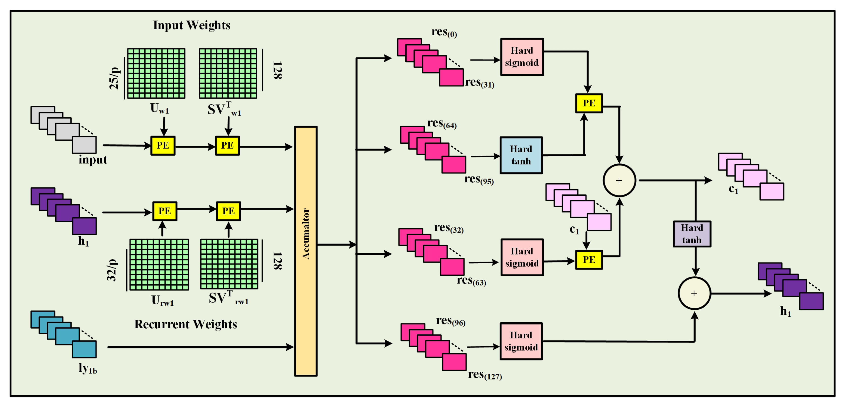
Figure 7 illustrates the internal architecture of the LSTM Layer-1 compute block optimized for hardware implementation. This unit processes three primary inputs: the current input, the previous hidden state ($h_1$), and a bias ($l{y}_{1b}$). These inputs are multiplied by their corresponding input and recurrent weights within specialized Processing Elements (PEs), after which the results are accumulated. The output is divided into four segments, each undergoing activation through functions such as hard sigmoid and hard tanh to compute the LSTM gates: the input gate, forget gate, output gate, and candidate cell state. The cell state ($c_1$) is then updated by calculating a weighted sum of the previous and new candidate cell states. Finally, the hidden state ($h_1$) is updated using the output gate in conjunction with the most recent cell state.

Figure 8 illustrates the detailed architecture of the LSTM Layer-2 compute block optimized for efficient pipelined hardware operation. In this layer, the design takes inputs as the hidden states from previous computations ($h_1$ and $h_2$) and a bias ($l{y}_{2b}$). Each input stream undergoes matrix multiplication with dedicated input and recurrent weights through Processing Elements (PEs). In contrast to Layer-1, this layer focuses on updating both the hidden state ($h_2$) and cell state ($c_2$) depending on the outcomes of numerous gate operations. The structure is built with a good accumulation and mixing mechanism for complex state transitioning over time. The availability of hard approximations of activations facilitates lower and easier hardware designs. So this architecture is appropriate for low-latency, high-throughput deep-stacked LSTM networks implemented on FPGA.

Algorithm 1 Proposed SVD-based low-rank optimized LSTM model

Require:  Define input size, hidden size, and output size. 1: Initialize weight matrices:       $U_{w1},U_{w2},U_{rw1},U_{rw2},$       $S{V}^{T}w1$, $S{V}^{T}w2$, $S{V}^{T}rw1$, $S{V}^{T}rw2$ 2: Initialize hidden states $h_1,h_2\leftarrow \mathbf{0}$ 3: Initialize cell states $c_1,c_2\leftarrow \mathbf{0}$ 4: for $l=1$ to 50 do 5:    Load input vector $x_l$ 6:    //H denotes hidden size 7:    // First LSTM Layer 8:    for $j=0$ to $4.H$ do 9:      $m_1\left[j\right]={\sum }_{k=0}^{25}{x}_l\left[k\right]·U_{w1}\left[j\right]\left[k\right]$ 10:      $m_2\left[j\right]={\sum }_{k=0}^{25}{m}_1\left[k\right]·S{V}_{w1}^T\left[j\right]\left[k\right]$ 11:      $m_3\left[j\right]={\sum }_{k=0}^H{h}_1\left[k\right]·U_{rw1}\left[j\right]\left[k\right]$ 12:      $m_4\left[j\right]={\sum }_{k=0}^H{m}_3\left[k\right]·S{V}_{rw1}^T\left[j\right]\left[k\right]$ 13:      $m_5\left[j\right]=m_2\left[j\right]+m_4\left[j\right]+l{y}_{1b}\left[j\right]$ 14:    end for 15:    // Gate Activations for Layer 1 16:    for $i=0$ to H do 17:      $i{p}_1\left[i\right]=\sigma \left(m_5[i+0·H]\right)$ 18:      $f{o}_1\left[i\right]=\sigma \left(m_5[i+1·H]\right)$ 19:      $c{e}_1\left[i\right]=tanh\left(m_5[i+2·H]\right)$ 20:      $o{u}_1\left[i\right]=\sigma \left(m_5[i+3·H]\right)$ 21:    end for 22:    // Update Layer 1 States 23:    for $i=0$ to H do 24:      $c_1\left[i\right]=f{o}_1\left[i\right]·c_1\left[i\right]+i{p}_1\left[i\right]·c{e}_1\left[i\right]$ 25:      $h_1\left[i\right]=o{u}_1\left[i\right]·tanh\left(c_1\left[i\right]\right)$ 26:    end for 27:    // Second LSTM Layer 28:    for $j=0$ to $4.H$ do 29:      $m_6\left[j\right]={\sum }_{k=0}^H{h}_1\left[k\right]·U_{w2}\left[j\right]\left[k\right]$ 30:      $m_7\left[j\right]={\sum }_{k=0}^H{m}_6\left[k\right]·S{V}_{w2}^T\left[j\right]\left[k\right]$ 31:      $m_8\left[j\right]={\sum }_{k=0}^H{h}_2\left[k\right]·U_{rw2}\left[j\right]\left[k\right]$ 32:      $m_9\left[j\right]={\sum }_{k=0}^H{m}_8\left[k\right]·S{V}_{rw2}^T\left[j\right]\left[k\right]$ 33:      $m_{10}\left[j\right]=m_7\left[j\right]+m_9\left[j\right]+l{y}_{2b}\left[j\right]$ 34:    end for 35:    // Gate Activations for Layer 2 36:    for $i=0$ to H do 37:      $i{p}_2\left[i\right]=\sigma \left(m_{10}[i+0·H]\right)$ 38:      $f{o}_2\left[i\right]=\sigma \left(m_{10}[i+1·H]\right)$ 39:      $c{e}_2\left[i\right]=tanh\left(m_{10}[i+2·H]\right)$ 40:      $o{u}_2\left[i\right]=\sigma \left(m_{10}[i+3·H]\right)$ 41:    end for 42:    // Update Layer 2 States 43:    for $i=0$ to H do 44:      $c_2\left[i\right]=f{o}_2\left[i\right]·c_2\left[i\right]+i{p}_2\left[i\right]·c{e}_2\left[i\right]$ 45:      $h_2\left[i\right]=o{u}_2\left[i\right]·tanh\left(c_2\left[i\right]\right)$ 46:    end for 47: end for 48: // Dense Output Layer 49: $dense\_out=\sum {i=0}^H{h}_2\left[i\right]·dw\left[i\right]$ 50: $dense\_out+=db$ 51: $y=\sigma (dense\_out)$ 52: return y

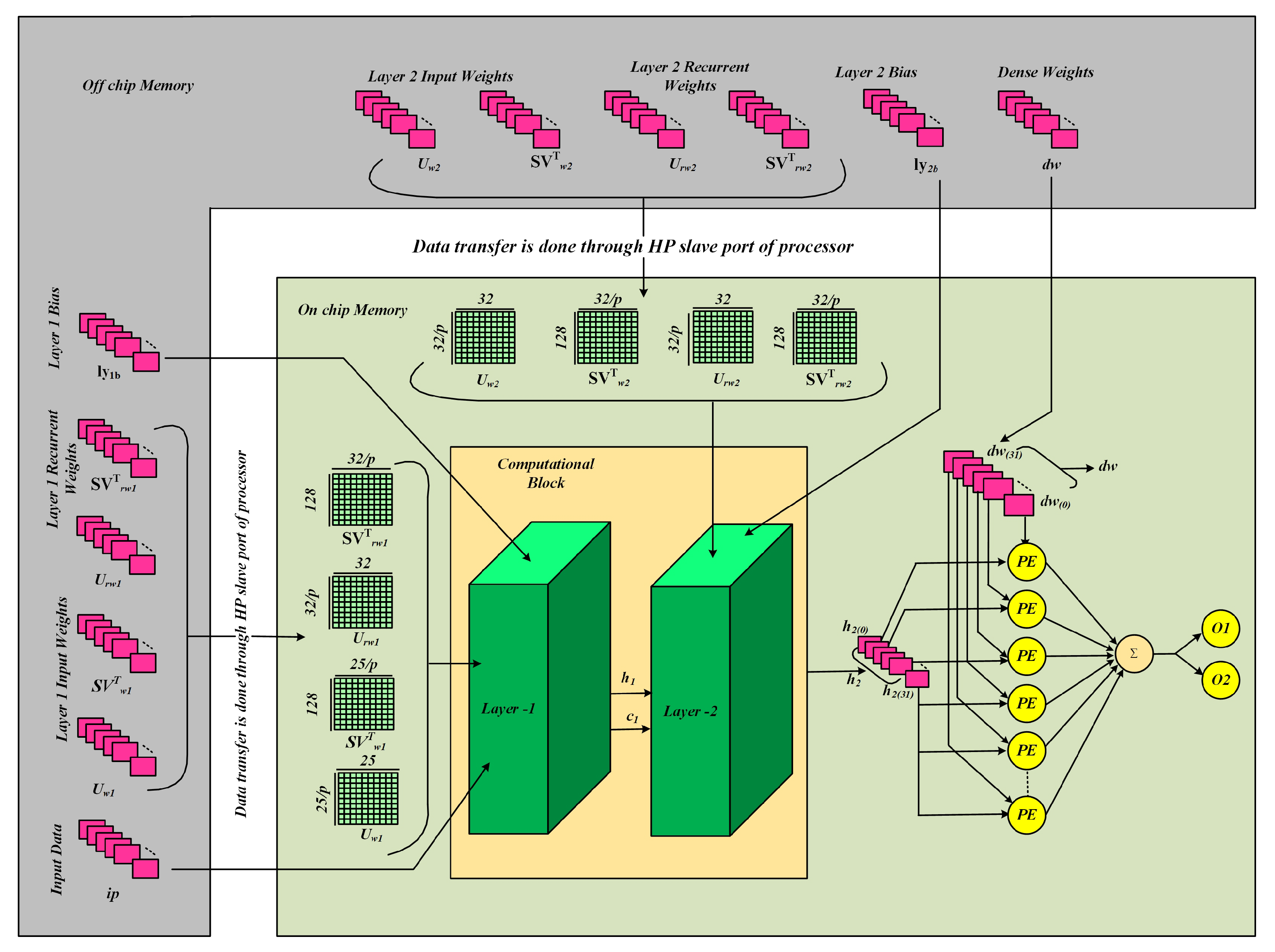
Figure 9 shows an overview of the two-layer LSTM hardware architecture tailored for optimized computation and data transport using both off-chip and on-chip memory resources. Input data (ip), in addition to the weights of Layer-1 input weights ($U_{w1}$), recurrent weights $(U_{rw1}$), transformation matrices ($S{V}_{w1}^T$, $S{V}_{rw1}^T$), and layer biases ($l{y}_{1b}$) are first written into off-chip memory. These parameters are passed through the HP slave port of the processor to on-chip memory to reduce latency at the time of computation. The computational block is formed of two consecutive LSTM layers. Layer-1 computes the input data and produces hidden ($h_1$) and cell states ($c_1$), which are sent to Layer-2 for subsequent computation. Similarly, Layer-2 takes its input weights ($U_{w2}$), recurrent weights ($U_{rw2}$), transformation matrices ($S{V}_{w2}^T$, $S{V}_{rw2}^T$), and biases ($l{y}_{2b}$) from off-chip memory through the processor interface. The final hidden state ($h_2$) is input into a dense layer after Layer-2 computation, where pre-computed dense weights ($dw$) are processed by numerous Processing Elements (PEs) in parallel to maximize throughput. The outputs from the PEs are summed, propagated through an activation function ($\sigma$), and ultimately yield the output nodes ($O1$, $O2$). This framework underscores proficient memory administration, utilizing parallel processing and hierarchical computation to enhance LSTM operations on hardware platforms.

The model uses 16-bit fixed-point arithmetic for weights, activations, and intermediate computations. This quantization format was chosen based on empirical trade-offs between model accuracy and resource efficiency, ensuring no significant degradation in classification accuracy compared to 32-bit floating point.

The U and $S{V}^T$ matrices are stored separately and reused via shared Processing Elements for matrix–vector multiplication, reducing memory access bottlenecks. The ∑ matrix is handled as a scaling vector to reduce multiplier complexity.

The control logic of the proposed FPGA architecture is structured into an outsider controller and an insider controller. The outsider controller manages data loading, initialization, and coordination between LSTM layers, ensuring smooth data flow from BRAM to computation units. The insider controller handles internal operations through a stage-wise finite state machine (FSM), where Stage 1 executes all computations for Layer 1, and Stage 2 processes Layer-2 using the outputs of Layer-1. This hierarchical control ensures synchronized, pipelined execution for efficient real-time inference.

Effective communication and data transfer mechanisms are essential for ensuring the proposed two-layer LSTM hardware architecture operates efficiently in real-time PdM optimized using SVD applications. The architecture relies on seamless interaction between the ZYNQ processor, off-chip memory (DDR), and the FPGA’s computational blocks to handle high-speed data streams and weight matrices. An AXI-based communication system handles control signals and data transfer to support low-latency and high-throughput performance. Section 5.1 explains the AXI-based communication architecture, detailing how it combines with the designed hardware model to facilitate robust and scalable real-time processing on the Xilinx ZCU-104 platform.

To minimize off-chip memory usage and latency, the weight matrices and SVD components are preloaded into BRAM through the AXI HP slave port. Weight reuse across time steps reduces DDR3 bandwidth demand, and no memory stalls were observed during the 50-timestep input sequence processing.

5.1. AXI-Based Communication in Proposed Architecture

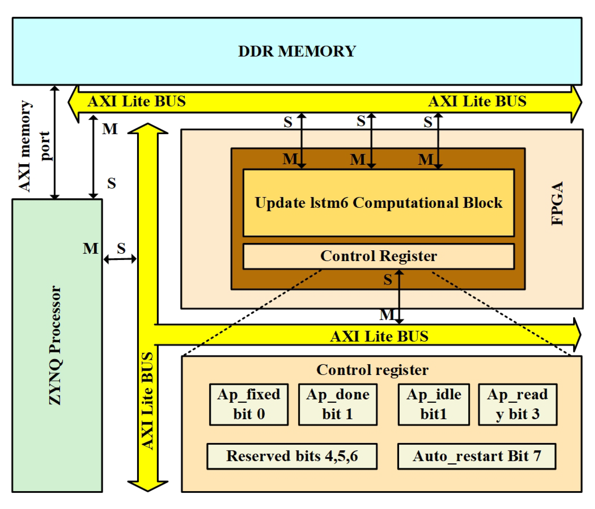
Figure 10 illustrates the communication structure between a ZYNQ processor and an off-the-shelf custom computation block running on an FPGA, utilizing AXI protocols. The ZYNQ processor is connected to the DDR memory via an AXI memory port and communicates with the FPGA through AXI Lite and AXI memory-mapped buses. Within the FPGA, the core computation block, referred to as the Update LSTM Computation Block, is managed by a control register that governs its operation. Lightweight control signal transfers are handled via the AXI Lite bus. In contrast, high-speed data transfers between the DDR memory and the FPGA computation block are managed by the AXI memory bus. The control register also provides necessary status signals, such as ap_fixed (bit 0), ap_done (bit 1), ap_idle (bit 2), and ap_ready (bit 3), and enables features like auto_restart (bit 7). Bits 4, 5, and 6 are reserved for future expansion or additional functionality. This design facilitates efficient management and execution of compute-intensive tasks, with synchronized control and high-speed data communication between the processor and FPGA logic.

5.2. End-to-End Implementation Flow for Proposed Model

The deployment of an LSTM model on a ZCU-104 FPGA board involves a synchronized three-phase parallel process, as depicted in Figure 11, encompassing software training, hardware design, and hardware implementation.

Software Level: The process started by opening interactive Python notebooks to preprocess and normalize the dataset, then training, validation, and testing the deep learning model on the CPU. The trained weights and biases obtained were stored in .npy files to be reused.

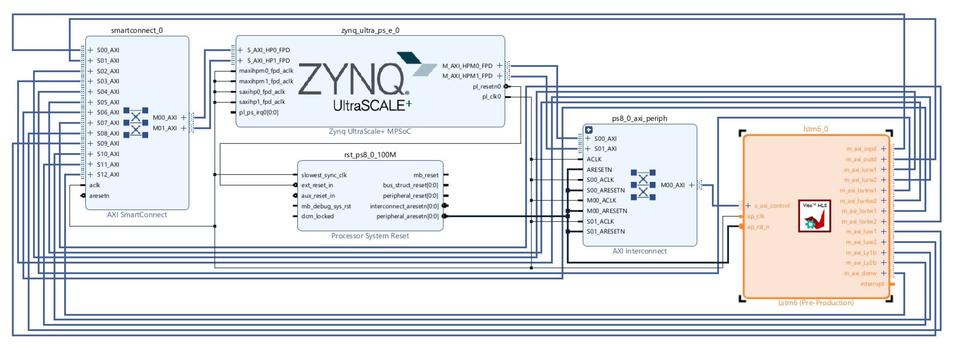
Hardware Design Level: Concurrently, C++ code was developed using Vivado HLS with pragma HLS methods. This underwent C synthesis, RTL export, and Verilog IP generation. In Vivado’s IP integrator, a block design integrated the Zynq processing system (PS) with the custom HLS IP (named Lstm6_0 in Figure 12), using SmartConnect AXI interconnects. Synthesis and implementation generated the target bitstream and supporting files (.bit, .hwh, .tcl).

Hardware Implementation Level: The ZCU-104 board was prepared by preloading its image onto a microSD card, booting it, and establishing an Ethernet connection. A Jupyter interface was accessed to load the hardware overlay. The stored weights and biases were mapped to memory buffers, with their physical addresses noted for FPGA utilization.

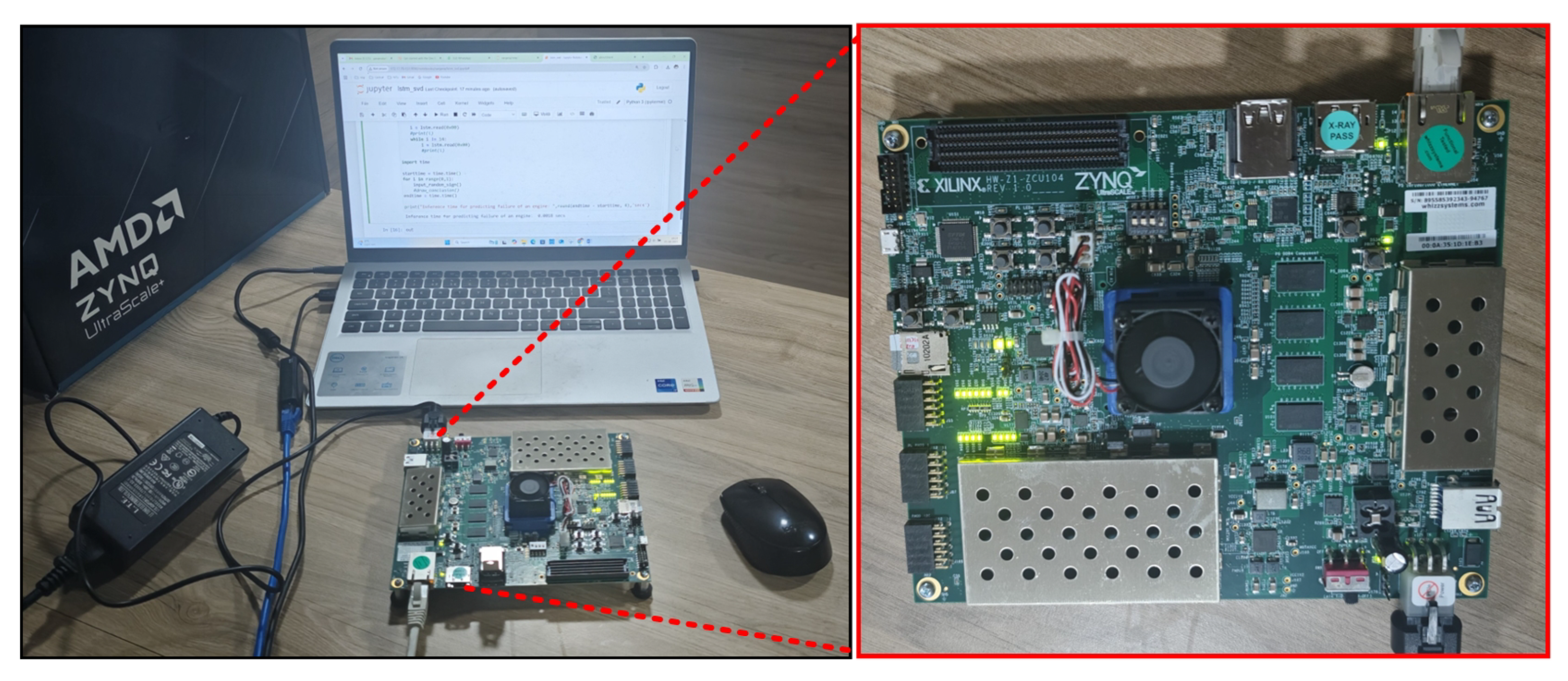
The hardware setup, shown in Figure 13, involves transferring the .bit, .hwh, and .tcl files of the SVD-LSTM model (designed with Vivado 2022.2) to the ZCU-104 via Ethernet, with power supplied through a USB cable. Aircraft sensor data (e.g., vibration or pressure time series) is loaded into DDR3 memory via a Jupyter Notebook 7.2.1 running on the ARM Cortex processor. An ap_start signal triggers the FPGA accelerator, which performs SVD-based compression and LSTM sequence modeling. Data is transferred from DDR3 to BRAM for computation, and the prediction results (e.g., remaining useful life or fault status) are written back to DDR3 for processor access and user display. The system co-design execution flow, as illustrated in Figure 14, involves the following steps:

($T_1$): Saving the aircraft sensor time-series input into DDR3 memory using the Jupyter notebook interface.

($T_3$): Transferring compressed SVD matrices, LSTM weights, and biases from DDR3 to BRAM.

($T_4$): The computed values of the two computing units are then transferred from BRAM to DDR3 memory.

($T_2$): Storing the predicted output in DDR3 memory for access by the processor.

($T_5$): The time taken by the processor to transfer all LSTM weights and biases associated with both compute units into the DDR3 memory.

As shown in Equation (18), the total time consumption of the system is 0.0018 s.

$$T_1+T_2+T_3+T_4=0.0018\sec$$

(18)

The ZCU-104 FPGA implementation efficiently processes thousands of samples with minimal latency, surpassing conventional CPU execution while preserving prediction accuracy. Its low power consumption makes it ideal for UAV deployment. It enables onboard predictive maintenance in resource-constrained environments, such as real-world avionics for real-time engine health monitoring during flight.

6. Experimental Results

The proposed work result analysis was done at both the software and hardware levels. First, software result analysis (like training and testing) is discussed, and then hardware result (resource utilization) analysis, including an ablation study, is discussed.

6.1. Software Result Analysis

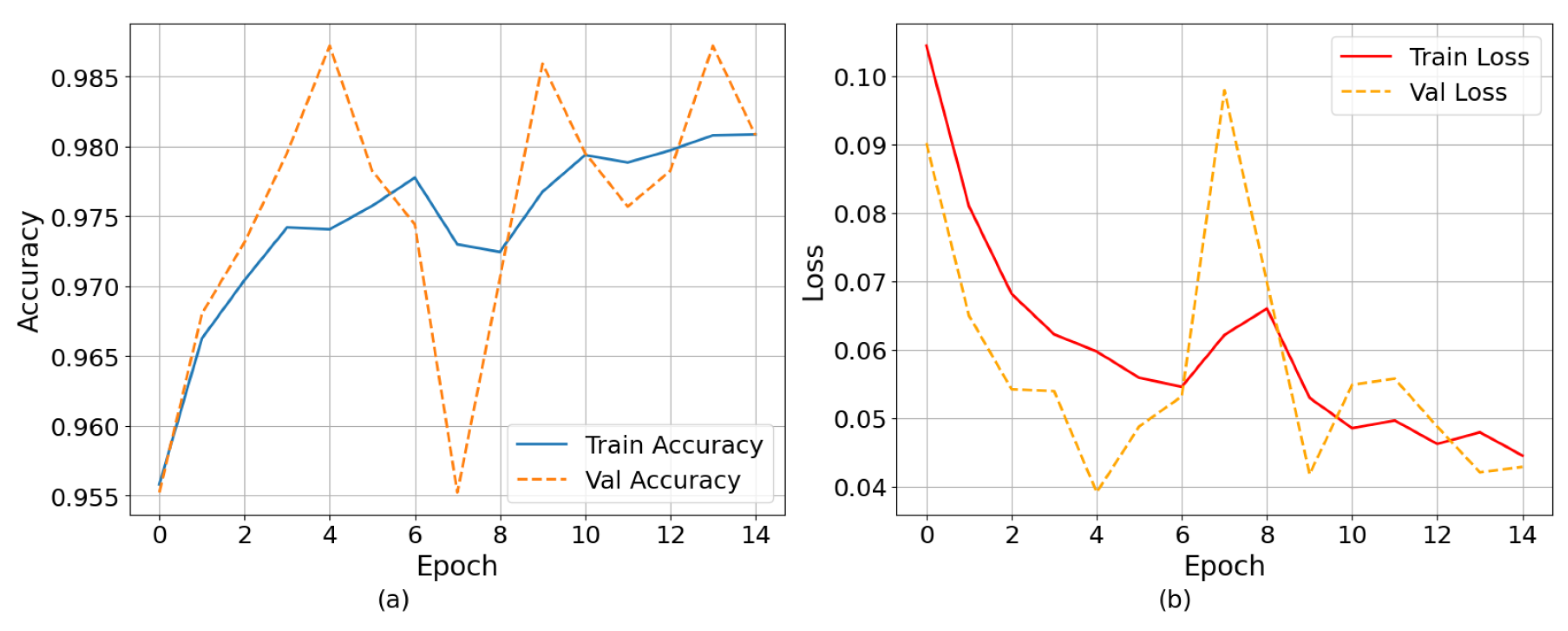
The training performance of the LSTM model is displayed in terms of accuracy and loss over epochs in Figure 15. The training accuracy increases steadily to 98.1%, and the validation accuracy reaches 98.7% with only minor variations, indicating strong generalization and minimal overfitting. Training and validation losses correspondingly drop from 0.105 and 0.09 to 0.04 and 0.043, respectively.

A four-fold cross-validation technique was used during the training phase to evaluate the robustness and generalization capacity of the proposed LSTM model. Four equal subsets of the dataset were created for this process; in each iteration, three subsets were used for training and the remaining subset was used for validation. This procedure was repeated four times to ensure that every data sample was used as a validation point just once. The model performed consistently across the folds, with a mean validation accuracy of 98.32% and a mean training accuracy of 98.48%.

In addition to visual inspection, performance metrics were calculated to assess the model’s classification capabilities quantitatively. The model achieved a test precision of 1.00, indicating a high proportion of correctly predicted positive samples among all optimistic predictions. The test recall was 0.92, reflecting the model’s ability to identify the majority of actual positive cases. Furthermore, the F1-score, which balances precision and recall, was 0.958. These metrics confirm that the model maintains strong generalization performance and effectively handles imbalanced or binary classification tasks. The model reported a prediction accuracy of 98%, and a comprehensive examination of the model’s error characteristics was performed to further understand its resilience and potential implications for flight safety. A primary issue in critical UAV engine monitoring applications is the risk of false negative instances where the system does not detect an imminent failure. Our model reported a false negative rate (FNR) of 4%, indicating that in 4% of positive failure cases, 4 out of every 100 potential engine failures may go undetected. This represents a critical safety concern in flight-critical UAV systems. However, this rate is relatively low compared to similar predictive maintenance models reported in the literature, suggesting the model’s suitability for early warning systems.

6.2. Hardware Result Analysis

To demonstrate how fixed-point arithmetic yields lower latency and less resource consumption than floating-point arithmetic, take a simple numerical example of multiplication. Let us say we are to multiply two numbers: 2.5 and 1.5. In a fixed-point system with a Q4.12 format (i.e., 4 bits for the integer part and 12 bits for the fractional part), these numbers are scaled up by $2^4=16$. Therefore, 2.5 is expressed as $2.5\times 16=40$, and 1.5 is expressed as $1.5\times 16=24$. Multiplying these two scaled integers results in

$$40\times 24=960$$

To return to the original scale, we divide the product by $2^4\times 2^4=256$, yielding

$${\displaystyle \frac{960}{256}}=3.75$$

which corresponds to the correct result of 3.75. This operation uses only simple integer multiplication and a bit shift for scaling, which is extremely efficient in hardware, requiring minimal clock cycles and logic.

In contrast, floating-point multiplication using the IEEE-754 32-bit format involves significantly more overhead. The number 2.5 is represented in binary as 0x40200000, and 1.5 is described as 0x3FC00000. To multiply these values, the system must align the exponents, then multiply the mantissas, normalize the result, handle any rounding, and reassemble the result into the standard floating-point format. Each step requires complex control logic and specialized arithmetic units such as floating-point multipliers and adders. These units consume more DSP slices, flip-flops, and lookup tables; each operation can take multiple clock cycles.

Fixed-point arithmetic optimizes hardware logic and accelerates execution speed, allowing the LSTM hardware implementation to decrease latency by 24% (from 84,945 to 64,475 cycles) and resource consumption (26% less BRAM, 37% less DSP) relative to a 32-bit floating-point SVD-compressed FPGA implementation, as illustrated in

Table 4. Resource utilization and latency analysis of both floating-point and fixed-point implementations.

Precision Type	Latency (in Cycles)	BRAM	DSP	FF	LUT
Floating point (32 bit)	84,945	269	506	96,462	80,702
Fixed point (16 bit)	64,475	198	316	38,322	44,388

. This efficiency extends UAV flight time and improves real-time fault tolerance, allowing low-latency inference that enables in-flight reactivity, which is crucial for preventing failures during autonomous navigation.

The floating-point baseline refers to a 32-bit compressed model deployed on the same ZCU-104 FPGA. This serves as a fair comparison to highlight the efficiency gained by fixed-point SVD-compressed deployment. Both the floating-point and fixed-point implementations use SVD-compressed LSTM models. The performance comparison isolates the impact of numerical precision, not SVD compression itself.

Figure 16 shows the impact of diverse Singular Value Decomposition (SVD) compression factors, labeled as p, on the percentage decrease of parameters across various weight matrices in a two-layer LSTM network. During Singular Value Decomposition (SVD), the compression factor p is the rank used to get close to the original weight matrix in its low-rank form. It has a direct effect on the level of compression. A smaller p-value means more compression with higher approximation error, while a larger p-value means less compression but more information retention. The X-axis shows the SVD compression factor p, which can be between 2 and 7, and the Y-axis shows the percentage of parameter reduction that goes with it. It is possible to divide weight matrices into four groups: Layer-1 input weights, Layer-1 recurrent weights, Layer-2 input weights, and Layer-2 recurrent weights. As p goes up, all types of weights show the same rise in parameter decrease. At p = 2, the drop is small, with Layer-1 input weights reaching 43% and the rest at 37%. At p = 3, they all undergo a 61% reduction, which means they are better at approximation. The trend continues; at p = 7, the most significant drop is 86% for Layer-1 input weights and 84% for the others. These results show that SVD compression can effectively lower parameters while keeping structure, especially after p = 3. It is a good way to improve LSTM models in places with limited resources, like FPGAs.

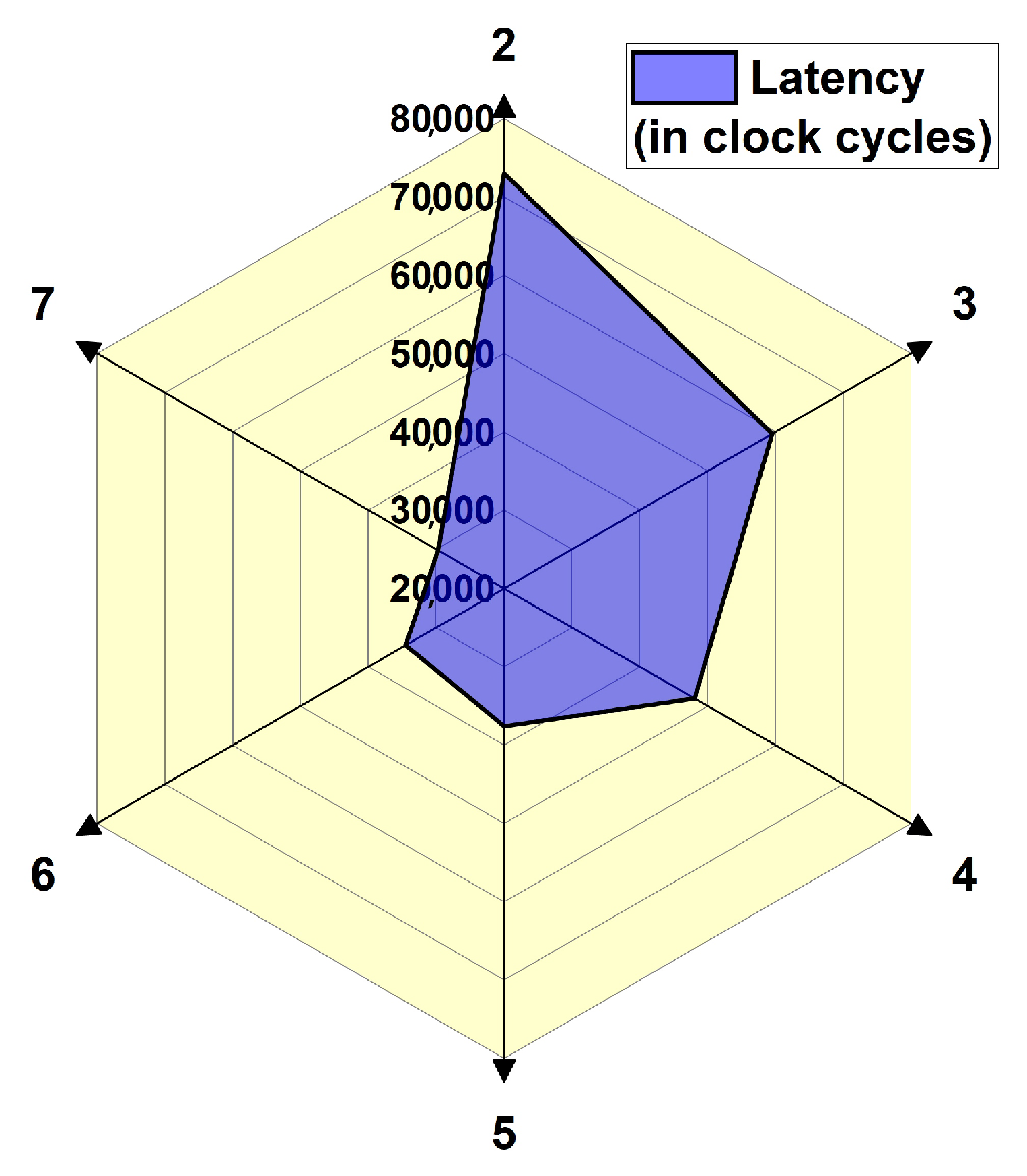
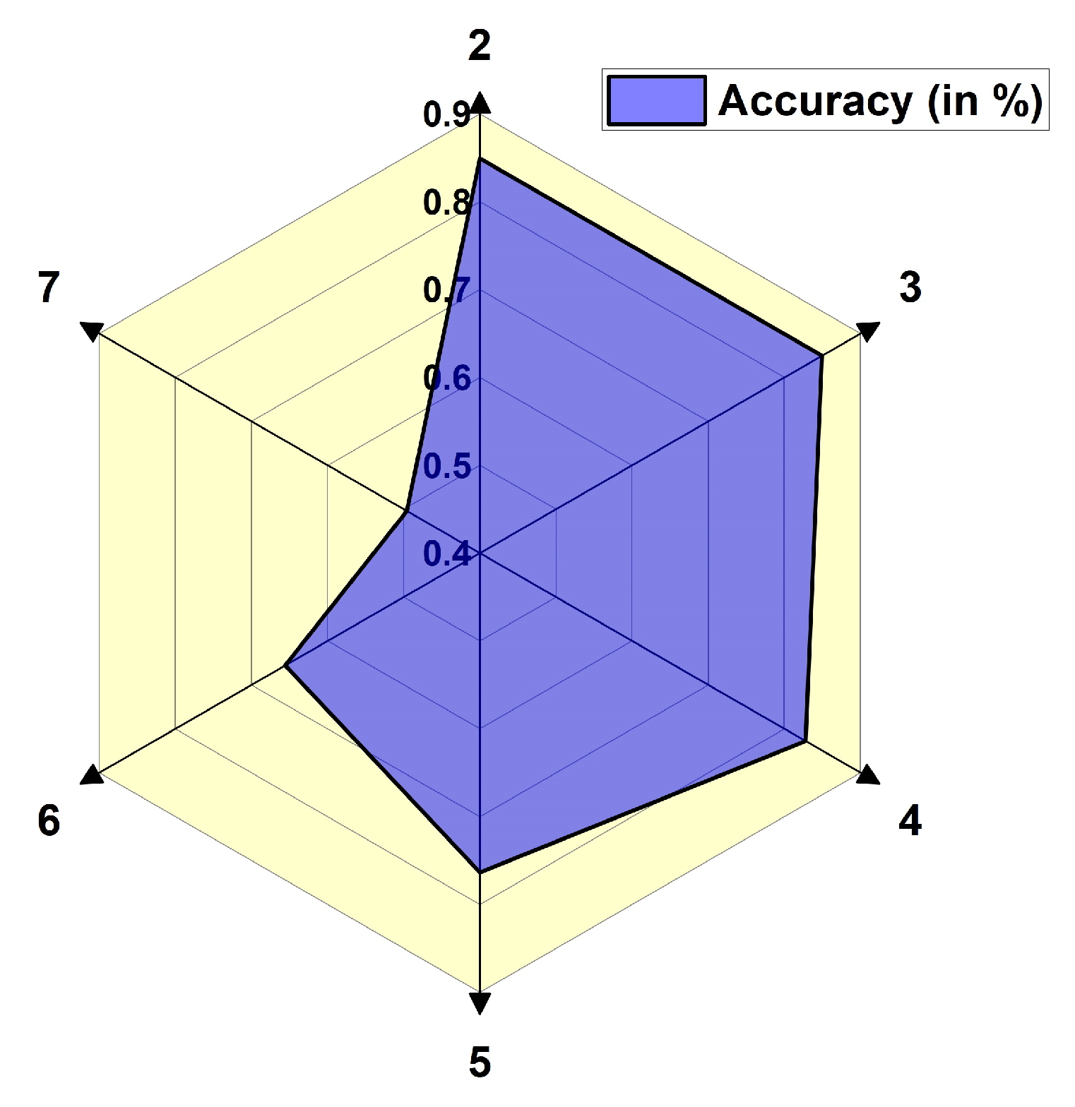
The latency results shown in Figure 17 are a semi-transparent blue-shaded surface, with each axis denoting a particular SVD compression factor value. Axis 2 (SVD compression factor = 2) shows significantly higher latency, exceeding roughly 75,000–80,000 clock cycles, indicating the highest time consumption for the smallest SVD compression factor. Conversely, latencies on axes 3 to 7 are relatively lower, ranging from 20,000 to 50,000 clock cycles, indicating greater efficiency in those configurations.

For instance, as shown in Figure 18, consider reducing the recurrent weight matrix in Layer 1 by a factor of 2. Retaining 16 singular values in a $32\times 128$ matrix where the maximum rank is 32 preserves approximately 84.9% of the original information content. Compression by a factor of 3 maintains a similar level of variance (84.95%), indicating that this level of reduction still captures the most significant characteristics. However, as the compression factor increases, the retained variance decreases: a compression factor of 4 retains 82.79%, factor 5 retains 76.34%, and factor 7 captures only 49.6% of the total variance. The observed accuracy illustrates the principle of diminishing returns in matrix compression, where the most pertinent information is concentrated in the largest singular vectors. Excessive compression, therefore, may lead to information loss.

6.3. Performance Analysis Between Software and Hardware Results

Table 5. Latency comparison between FPGA and CPU implementations.

IP Name	FPGA (ms)	CPU (ms)
LSTM	0.084945	90

presents a comparison of the latency between FPGA and CPU implementations for the proposed LSTM model. The latency on FPGA is just 0.084945 milliseconds, whereas the CPU takes 90 milliseconds to process the same task. This demonstrates a significant speedup of over 1000 times offered by the FPGA. Such performance improvement highlights the suitability of hardware acceleration for real-time and embedded applications, where low latency is critical for responsiveness and efficiency.

7. Comparative Analysis

Recently, advancements in predicting the requirements of aviation engines have demonstrated impressive success in adopting a few deep learning paradigms. The study utilized a sophisticated neural network design and innovative data augmentation techniques to attain an accuracy rate of 98% [28]. The survey introduced an innovative hybrid architecture that combines the attention mechanism with deep learning models, resulting in a prediction accuracy of 97% [29]. The present study achieves an accuracy rate of 98%, significantly outperforming all previously reported models. The enhancement in predicted accuracy underscores the robustness, adaptability, and remarkable generalization capacity of the proposed method, making it a very reliable device for aircraft engine health assessment and precise calculation of remaining useful life. These enhancements signify a substantial advancement in guaranteeing the safety, efficiency, and cost-effectiveness of aircraft maintenance operations.

The present study achieves an accuracy of 98%, which is equivalent to or superior to previous models. The proposed model demonstrates strong generalization capabilities, maintaining steady performance on both training and unseen validation sets, as seen by a minimal loss gap and consistent accuracy trends. Singular Value Decomposition (SVD) is utilized to significantly diminish the dimensionality of the model’s weight matrix, leading to a considerable decrease in computational complexity while maintaining performance consistency. This compression facilitates outstanding scalability, allowing the model to function effectively with minimal hardware resources. Such optimizations render the model highly deployable in real-world aviation settings, with computational requirements, noisy data, and high response times. Integrating deep learning, SVD-based optimization, and FPGA-based acceleration provides a robust, flexible, and feasible solution for predictive maintenance and health monitoring of advanced aircraft engines.

A comparison of existing LSTM compression and hardware deployment strategies is summarized in

Table 6. Model compression, hardware, and performance summary.

Author	Compression Method	Hardware & Platform	Application	Accuracy/Metric	Latency
Gao et al. (2022) [30]	Structured pruning, DeltaLSTM (spatio-temporal)	FPGA (unspecified)	Speech recognition	Negligible accuracy loss (~94% sparsity)	~1 µs per LSTM layer
Wang et al. (2018) [31]	Block-circulant compression, 16-bit quantization	FPGA	Acoustic recognition	Small accuracy degradation	18.8× speedup vs. baseline
Han et al. (2016) [32]	Load-balanced pruning, quantization	Xilinx XCKU060 FPGA	Speech recognition	No accuracy drop	Full LSTM at 282 GOPS
Wang et al. (2022) [33]	Structured pruning, mixed-precision quantization	FPGA (unspecified)	Meta-learning LSTM	±0.2% accuracy change	50× energy-efficiency boost
Mshragi et al. (2025) [34]	NAS, quantization	Pynq Z1 FPGA	Building management systems	MSE: 0.00018	~2.6 ms per inference
Hayajneh et al. (2023) [35]	LSTM unit reduction	UAV Edge (unspecified)	Soil moisture prediction	$R^2>0.999$	Reduced latency with smaller model
Proposed SVD-LSTM (2025)	SVD-based compression + fixed-point inference	Xilinx ZCU-104 FPGA	UAV engine health classification	98% classification accuracy	0.085 ms (85 µs)

. Most rely on pruning, quantization, or simplified architectures. However, none of these approaches applies SVD compression in an FPGA setup for aviation use cases, making this work a novel contribution to real-time, resource-efficient predictive maintenance.

8. Conclusions

This study created a practical hardware-accelerated predictive maintenance framework for UAV engines. It uses an SVD-based LSTM running on an FPGA. While previous studies have primarily focused on the regression-based estimation of RUL, this work reframes the problem as a binary classification task using RUL thresholds. This formulation enables the deployment of models in real time on an FPGA, allowing for earlier and more useful predictions that are crucial for making informed decisions in flight. This method enables UAVs to perform PdM in the field, eliminating the need for ground communication systems and allowing them to operate independently in challenging or remote areas. The Xilinx ZCU-104 FPGA used in this work operates well within temperatures ranging from −40 °C to +85 °C, which is suitable for locations with high altitudes where temperature fluctuations are common. The suggested system uses low-power 16-bit fixed-point arithmetic and optimized memory access patterns. This reduces power consumption and ensures that power remains stable in environments where power is not always consistent, which is very common in UAV setups. The AXI architecture-based FPGA setup works well with standard UAV avionics systems when combined with the Zynq processor. The model weights and SVD matrices are stored in on-chip memory (BRAM). This helps lower the demand on memory bandwidth, which keeps data transfers from being delayed, even when the UAV moves quickly or the environment changes quickly. We conducted numerous ablation studies with various SVD compression factors to determine the optimal balance between accuracy and speed. These studies also evaluated the model’s performance and the hardware resource utilization across different compression levels. Due to its real-time inference capability, low-latency edge deployment, and is adaptability, the proposed SVD-compressed LSTM model running on an FPGA is ideal for use in a Digital Twin (DT) framework. An effective hardware accelerator was designed to handle both floating-point and 16-bit fixed-point computations. On the Xilinx ZCU-104 platform, the fixed-point design achieved a 24% decrease in latency, a 26% reduction in BRAM usage, and a 37% decrease in DSP utilization. The pipelined AXI-based hardware architecture makes sure that the system responds in real-time by optimizing memory access. This allows for continuous monitoring while the system is in flight. While not explicitly targeting avionics certification standards, the system’s deterministic latency and robust embedded execution make it a strong candidate for integration into Digital Twin (DT) frameworks and real-world UAV maintenance systems. Further, the future work will involve evaluating GPU-based edge devices for predictive maintenance tasks and conducting a comparative analysis of FPGA and GPU implementations. This will provide a clearer understanding of hardware choices for UAV applications in future deployments.

9. Future Scope

Future model advancements might include advanced compression methods, including pruning, quantization-aware training, and knowledge distillation, to improve inference performance and reduce hardware resource utilization. Enhancing the system to facilitate multi-fault detection and real-time adaptive learning from streaming sensor data would improve its robustness and intelligence. In the future, we might test the framework in real-world flight situations or combine it with Digital Twin frameworks for UAV fleets to see how well it works in real-world situations and make it more useful for a wider range of missions. Using next-generation FPGA platforms could make things a lot more scalable and efficient, making them more useful in commercial aviation and a number of industrial predictive maintenance applications.