

Evaluating the Potential of UAVs for Monitoring Fine-Scale Restoration Efforts in Hydroelectric Reservoirs

 ,
,
Abstract
1. Introduction
- Understanding specific flight parameters that are best suited to collect data in a barren beach environment where there is little elevation change or obstacles but the vegetation is relatively small;
- Determining how LiDAR versus photogrammetry data perform in this specific environment and task;
- Understanding how the information collected from this study can be used to inform future UAV data collection.
2. Materials and Methods
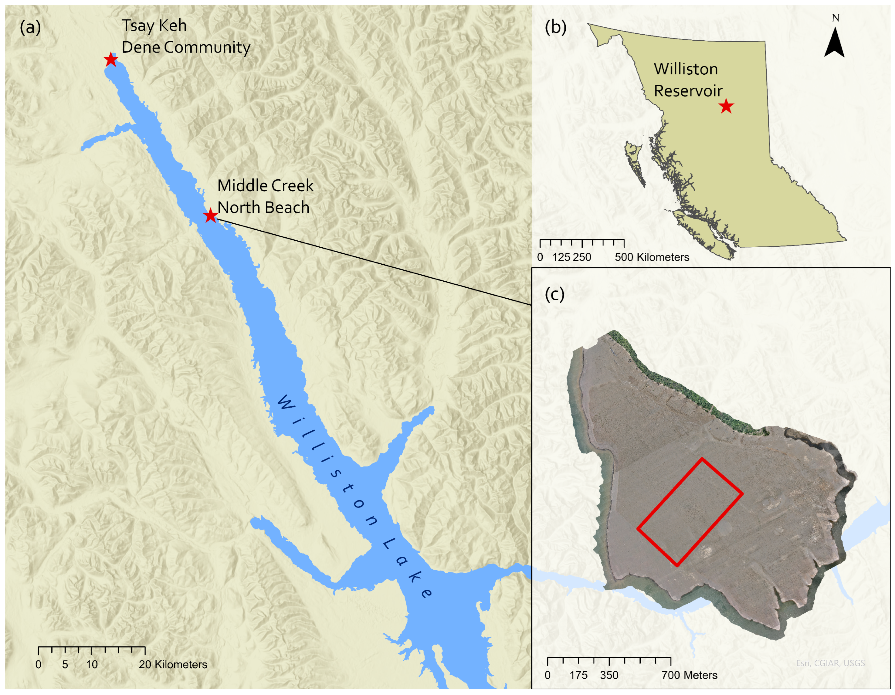
2.1. Study Area
2.2. Data Collection
2.2.1. LiDAR Flights
2.2.2. Photogrammetry Flights
2.2.3. Ground Truthing
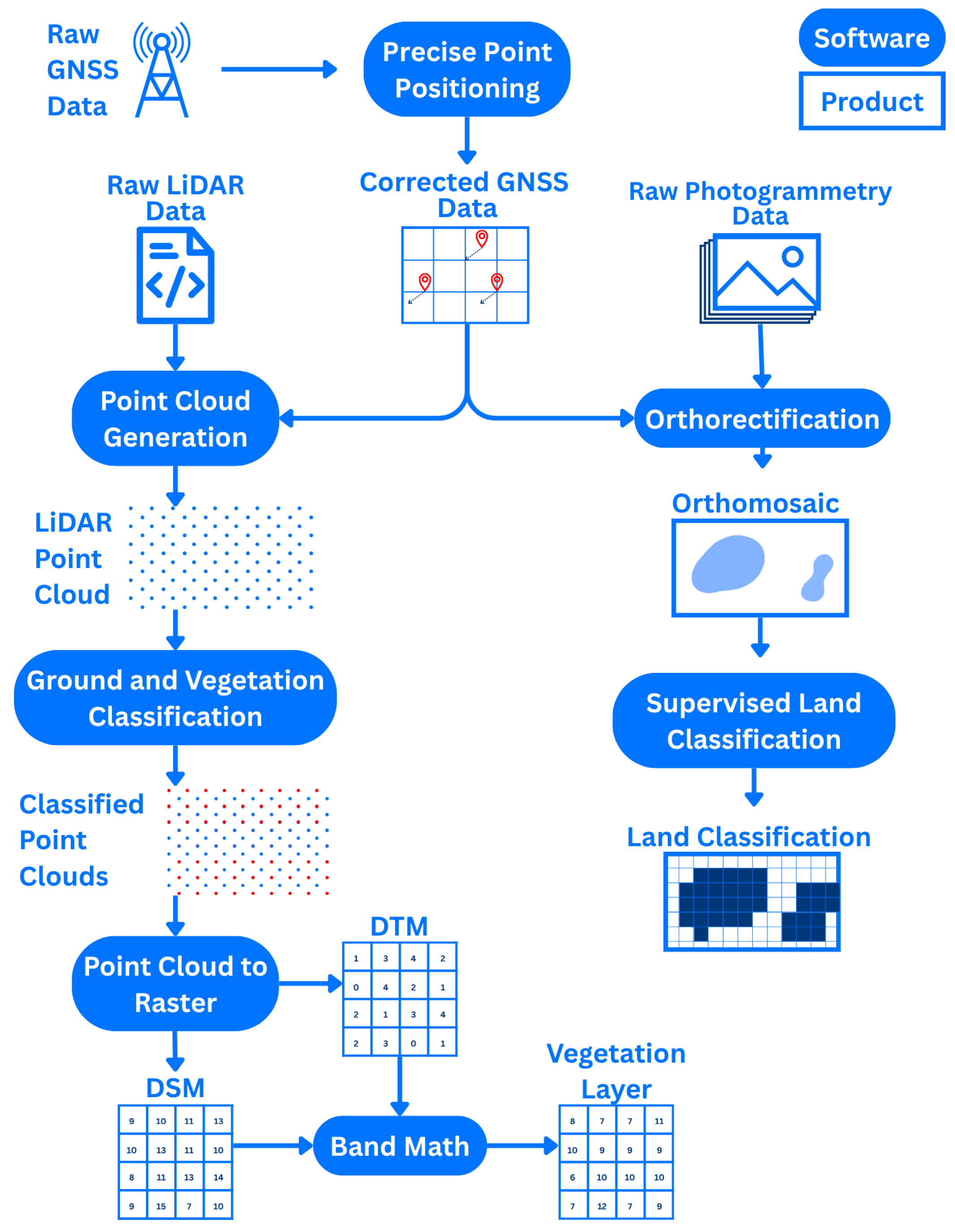
2.3. Processing
2.3.1. LiDAR
2.3.2. Photogrammetry
2.3.3. Comparison
3. Results
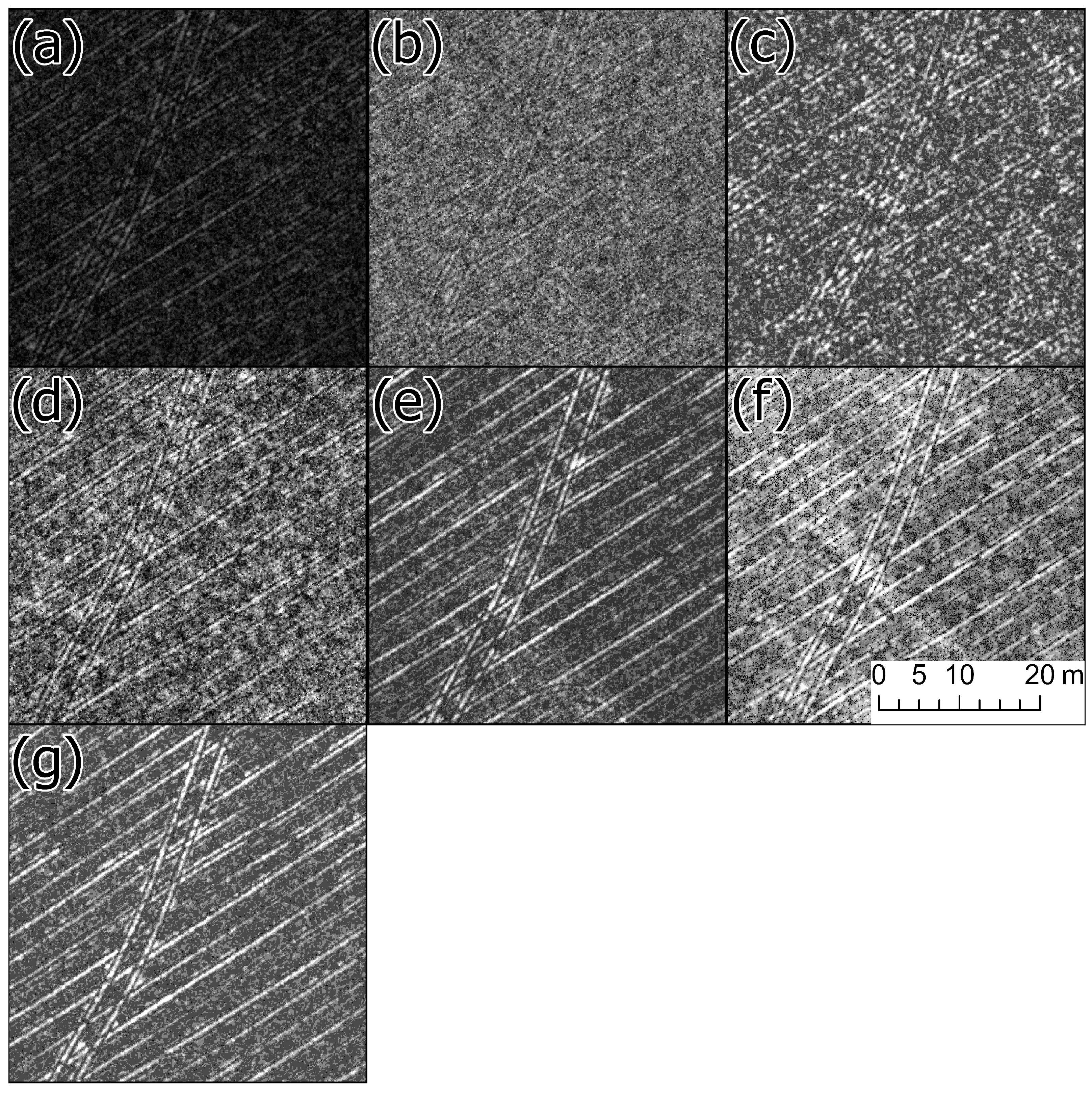
3.1. LiDAR
Photogrammetry
4. Discussion
Limitations
5. Conclusions
- For vegetation of this size (10 cm high grasses) to be monitored over a large area, photogrammetry is a better-suited instrument than LiDAR as the small-scale vegetation is too easily lost in the noise of the LiDAR.
- The altitude of the flight was the most impactful parameter for improving the quality of the results for both photogrammetry and LiDAR.
Author Contributions
Funding
Institutional Review Board Statement
Informed Consent Statement
Data Availability Statement
DURC Statement
Acknowledgments
Conflicts of Interest
References
- Hydroelectricity Generation Dries Up Amid Low Precipitation and Record High Temperatures: Electricity Year in Review 2023; Statistics Canada: Ottawa, ON, Canada, 2024.
- BACKGROUNDER: BC’s Energy System; Government of British Columbia: Victoria, BC, Canada, 2024.
- Wu, W.; Eamen, L.; Dandy, G.; Razavi, S.; Kuczera, G.; Maier, H.R. Beyond engineering: A review of reservoir management through the lens of wickedness, competing objectives and uncertainty. Environ. Model. Softw. 2023, 167, 105777. [Google Scholar] [CrossRef]
- Dams and Development: A New Framework for Decision-Making; Earthscan: Abingdon, UK, 2013; Backup Publisher: World Commission on Dams.
- Olsson, G. Water and Energy: Threats and Opportunities, 2nd ed.; IWA Publishing: London, UK, 2015. [Google Scholar]
- Darghouth, S.; Ward, C.; Gambarelli, G.; Styger, E.; Roux, J. Watershed Management Approaches, Policies, and Operations: Lessons for Scaling Up; World Bank: Washington, DC, USA, 2008; Volume 11. [Google Scholar]
- Willett, C.D.; Adams, M.J.; Johnson, S.A.; Seville, J.P. Capillary bridges between two spherical bodies. Langmuir 2000, 16, 9396–9405. [Google Scholar] [CrossRef]
- Kinbasket Reservoir: Dust; BC Hydro: Vancouver, BC, Canada, 2010.
- Williston Dust Control Trials and Monitoring; BC Hydro: Vancouver, BC, Canada, 2016.
- Carpenter Reservoir Drawdown Zone Riparian Enhancement Program 2020 Yearly Report; BC Hydro: Vancouver, BC, Canada, 2021.
- Giannadaki, D.; Pozzer, A.; Lelieveld, J. Modeled global effects of airborne desert dust on air quality and premature mortality. Atmos. Chem. Phys. 2014, 14, 957–968. [Google Scholar] [CrossRef]
- Derbyshire, E. Natural Minerogenic Dust and Human Health. AMBIO J. Hum. Environ. 2007, 36, 73–77. [Google Scholar] [CrossRef]
- Middleton, N.; Kang, U. Sand and dust storms: Impact mitigation. Sustainability 2017, 9, 1053. [Google Scholar] [CrossRef]
- Zhang, K.; Tang, C.S.; Jiang, N.J.; Pan, X.H.; Liu, B.; Wang, Y.J.; Shi, B. Microbial-induced carbonate precipitation (MICP) technology: A review on the fundamentals and engineering applications. Environ. Earth Sci. 2023, 82, 229. [Google Scholar] [CrossRef]
- Webb, N.P.; McCord, S.E.; Edwards, B.L.; Herrick, J.E.; Kachergis, E.; Okin, G.S.; Van Zee, J.W. Vegetation Canopy Gap Size and Height: Critical Indicators for Wind Erosion Monitoring and Management. Rangel. Ecol. Manag. 2021, 76, 78–83. [Google Scholar] [CrossRef]
- Maleki, S.; Miri, A.; Rahdari, V.; Dragovich, D. A method to select sites for sand and dust storm source mitigation: case study in the Sistan region of southeast Iran. J. Environ. Plan. Manag. 2021, 64, 2192–2213. [Google Scholar] [CrossRef]
- Su, Y.; Zhang, Y.; Wang, H.; Zhang, T. Effects of vegetation spatial pattern on erosion and sediment particle sorting in the loess convex hillslope. Sci. Rep. 2022, 12, 14187. [Google Scholar] [CrossRef]
- Zomorodian, S.M.A.; Ghaffari, H.; O’Kelly, B.C. Stabilisation of crustal sand layer using biocementation technique for wind erosion control. Aeolian Res. 2019, 40, 34–41. [Google Scholar] [CrossRef]
- Betz, F.; Halik, Ü.; Kuba, M.; Tayierjiang, A.; Cyffka, B. Controls on aeolian sediment dynamics by natural riparian vegetation in the Eastern Tarim Basin, NW China. Aeolian Res. 2015, 18, 23–34. [Google Scholar] [CrossRef]
- Auestad, I.; Nilsen, Y.; Rydgren, K. Environmental Restoration in Hydropower Development—Lessons from Norway. Sustainability 2018, 10, 3358. [Google Scholar] [CrossRef]
- Harada, J.; Yasuda, N. Conservation and improvement of the environment in dam reservoirs. Int. J. Water Resour. Dev. 2004, 20, 77–96. [Google Scholar] [CrossRef]
- Ancin-Murguzur, F.J.; Munoz, L.; Monz, C.; Hausner, V.H. Drones as a tool to monitor human impacts and vegetation changes in parks and protected areas. Remote Sens. Ecol. Conserv. 2020, 6, 105–113. [Google Scholar] [CrossRef]
- Qubaa, A.R.; Aljawwadi, T.A.; Hamdoon, A.N.; Mohammed, R.M. Using UAVs/Drones and vegetation indices in the visible spectrum to monitoring agricultural lands. Iraqi J. Agric. Sci. 2021, 52, 601–610. [Google Scholar] [CrossRef]
- Hama, A.; Tanaka, K.; Chen, B.; Kondoh, A. Examination of appropriate observation time and correction of vegetation index for drone-based crop monitoring. J. Agric. Meteorol. 2021, 77, 200–209. [Google Scholar] [CrossRef]
- Atanasov, A.; Mihaylov, R.; Stoyanov, S.; Mihaylova, D.; Benov, P. Drone-based Monitoring of Sunflower Crops. Annu. J. Tech. Univ. Varna Bulg. 2022, 6, 1–9. [Google Scholar] [CrossRef]
- Pérez-Luque, A.J.; Ramos-Font, M.E.; Tognetti Barbieri, M.J.; Tarragona Pérez, C.; Calvo Renta, G.; Robles Cruz, A.B. Vegetation Cover Estimation in Semi-Arid Shrublands after Prescribed Burning: Field-Ground and Drone Image Comparison. Drones 2022, 6, 370. [Google Scholar] [CrossRef]
- Sankey, T.; Donager, J.; McVay, J.; Sankey, J.B. UAV lidar and hyperspectral fusion for forest monitoring in the southwestern USA. Remote Sens. Environ. 2017, 195, 30–43. [Google Scholar] [CrossRef]
- Gonçalves, G.; Andriolo, U.; Gonçalves, L.M.; Sobral, P.; Bessa, F. Beach litter survey by drones: Mini-review and discussion of a potential standardization. Environ. Pollut. 2022, 315, 120370. [Google Scholar] [CrossRef]
- Stanley, M. Voices from Two Rivers: Harnessing the Power of the Peace and Columbia; Douglas & McIntyre: Vancouver, BC, Canada, 2010. [Google Scholar]
- DJI. Support for Matrice 300 RTK [Web Page]; SZ DJI Technology Co., Ltd.: Shenzhen, China, 2025; Available online: https://www.dji.com/support/product/matrice-300 (accessed on 5 July 2025).
- DJI Terra, Version 4.0 [Computer Software]; SZ DJI Technology Co., Ltd.: Shenzhen, China, 2024. Available online: https://www.dji.com/dji-terra (accessed on 5 July 2025).
- TerraScan. TerraSolid, Version 0.023.005 [Computer Software]; TerraSolid Ltd.: Helsinki, Finland, 2025. Available online: https://terrasolid.com/terrascan/ (accessed on 5 July 2025).
- ArcGIS Pro, Version 3.0 [Computer Software]; Environmental Systems Research Institute: Redlands, CA, USA, 2022. Available online: https://www.esri.com/en-us/arcgis/products/arcgis-pro/overview (accessed on 5 July 2025).
- Abdullah Abbas, H.; Sabah Jaber, H. Accuracy Assessment of land use maps classification based on remote sensing and GIS techniques. BIO Web Conf. 2024, 97, 00063. [Google Scholar] [CrossRef]
- Team, R.C. R: A Language and Environment for Statistical Computing; R Foundation for Statistical Computing: Vienna, Austria, 2024. [Google Scholar]
- Kuhn, M. Building Predictive Models in R Using the caret Package. J. Stat. Softw. 2018, 28, 1–26. [Google Scholar]
- Kuhn, M. caret: Classification and Regression Training (Version 7.0-1) [R Package]. 2024. Available online: https://CRAN.R-project.org/package=caret (accessed on 5 July 2025).
- Cohen, J. A Coefficient of Agreement for Nominal Scales. Educ. Psychol. Meas. 1960, 20, 37–46. [Google Scholar] [CrossRef]
- Cohen, J. Statistical Power Analysis for the Behavioral Sciences, 2nd ed.; Routledge: London, UK, 2013. [Google Scholar] [CrossRef]
- Pirotti, F.; Guarnieri, A.; Vettore, A. Ground filtering and vegetation mapping using multi-return terrestrial laser scanning. ISPRS J. Photogramm. Remote Sens. 2013, 76, 56–63. [Google Scholar] [CrossRef]
- Storch, M.; Kisliuk, B.; Jarmer, T.; Waske, B.; de Lange, N. Comparative analysis of UAV-based LiDAR and photogrammetric systems for the detection of terrain anomalies in a historical conflict landscape. Sci. Remote Sens. 2025, 11, 100191. [Google Scholar] [CrossRef]
- Guan, T.; Shen, Y.; Wang, Y.; Zhang, P.; Wang, R.; Yan, F. Advancing Forest Plot Surveys: A Comparative Study of Visual vs. LiDAR SLAM Technologies. Forests 2024, 15, 2083. [Google Scholar] [CrossRef]
- Man, Q.; Yang, X.; Liu, H.; Zhang, B.; Dong, P.; Wu, J.; Liu, C.; Han, C.; Zhou, C.; Tan, Z.; et al. Comparison of UAV-Based LiDAR and Photogrammetric Point Cloud for Individual Tree Species Classification of Urban Areas. Remote Sens. 2025, 17, 1212. [Google Scholar] [CrossRef]
- Oldeland, J.; Revermann, R.; Luther-Mosebach, J.; Buttschardt, T.; Lehmann, J.R. New tools for old problems—Comparing drone- and field-based assessments of a problematic plant species. Environ. Monit. Assess. 2021, 193, 90. [Google Scholar] [CrossRef]
- Mora-Felix, Z.D.; Sanhouse-Garcia, A.J.; Bustos-Terrones, Y.A.; Loaiza, J.G.; Monjardin-Armenta, S.A.; Rangel-Peraza, J.G. Effect of photogrammetric RPAS flight parameters on plani-altimetric accuracy of DTM. Open Geosci. 2020, 12, 1017–1035. [Google Scholar] [CrossRef]
- Seifert, E.; Seifert, S.; Vogt, H.; Drew, D.; van Aardt, J.; Kunneke, A.; Seifert, T. Influence of drone altitude, image overlap, and optical sensor resolution on multi-view reconstruction of forest images. Remote Sens. 2019, 11, 1252. [Google Scholar] [CrossRef]


| Test Variable | Altitude (m) | Speed (m/s) | Sidelap (%) | Point Cloud Density (points/m2) | GSD (cm/pixel) |
|---|---|---|---|---|---|
| Lower altitude | 50 | 6 | 30 | 479 | 1.36 |
| Slower speed | 100 | 3 | 30 | 472 | 2.73 |
| High sidelap | 100 | 12 | 60 | 239 | 2.73 |
| Lower altitude and higher sidelap | 50 | 6 | 60 | 963 | 1.36 |
| Lower altitude and slower speed | 50 | 3 | 30 | 943 | 1.36 |
| Higher sidelap and slower speed | 100 | 3 | 60 | 947 | 2.73 |
| Lower altitude and higher sidelap & Slower Speed | 50 | 3 | 60 | 1894 | 1.36 |
| Test Variable | Altitude (m) | Speed (m/s) | Sidelap (%) | GSD (cm/pixel) |
|---|---|---|---|---|
| Lower altitude | 50 | 7 | 70 | 0.63 |
| Slower speed | 100 | 3 | 70 | 1.26 |
| Lower altitude and slower speed | 50 | 3 | 70 | 0.63 |
| Threshold | True Veg | False Veg | True Sand | False Sand | Kappa | Accuracy |
|---|---|---|---|---|---|---|
| 0 | 43 | 32 | 68 | 57 | 0.11 | 0.555 |
| 10 | 38 | 28 | 72 | 62 | 0.1 | 0.55 |
| 20 | 3 | 5 | 95 | 92 | 0.03 | 0.515 |
| 30 | 1 | 0 | 100 | 99 | 0.01 | 0.055 |
| 40 | 0 | 0 | 100 | 100 | 0 | 0.5 |
| 50 | 0 | 0 | 100 | 100 | 0 | 0.5 |
| Flight | True Veg | False Veg | True Sand | False Sand | Kappa | Accuracy |
|---|---|---|---|---|---|---|
| Low | 100 | 3 | 97 | 0 | 0.97 | 0.985 |
| Slow | 86 | 2 | 98 | 14 | 0.84 | 0.92 |
| Low & Slow | 87 | 5 | 95 | 13 | 0.82 | 0.91 |
Disclaimer/Publisher’s Note: The statements, opinions and data contained in all publications are solely those of the individual author(s) and contributor(s) and not of MDPI and/or the editor(s). MDPI and/or the editor(s) disclaim responsibility for any injury to people or property resulting from any ideas, methods, instructions or products referred to in the content. |
© 2025 by the authors. Licensee MDPI, Basel, Switzerland. This article is an open access article distributed under the terms and conditions of the Creative Commons Attribution (CC BY) license (https://creativecommons.org/licenses/by/4.0/).
Share and Cite
Voss, G.; May, M.; Shackelford, N.; Kelley, J.; Stephen, R.; Bone, C. Evaluating the Potential of UAVs for Monitoring Fine-Scale Restoration Efforts in Hydroelectric Reservoirs. Drones 2025, 9, 488. https://doi.org/10.3390/drones9070488
Voss G, May M, Shackelford N, Kelley J, Stephen R, Bone C. Evaluating the Potential of UAVs for Monitoring Fine-Scale Restoration Efforts in Hydroelectric Reservoirs. Drones. 2025; 9(7):488. https://doi.org/10.3390/drones9070488
Chicago/Turabian StyleVoss, Gillian, Micah May, Nancy Shackelford, Jason Kelley, Roger Stephen, and Christopher Bone. 2025. "Evaluating the Potential of UAVs for Monitoring Fine-Scale Restoration Efforts in Hydroelectric Reservoirs" Drones 9, no. 7: 488. https://doi.org/10.3390/drones9070488
APA StyleVoss, G., May, M., Shackelford, N., Kelley, J., Stephen, R., & Bone, C. (2025). Evaluating the Potential of UAVs for Monitoring Fine-Scale Restoration Efforts in Hydroelectric Reservoirs. Drones, 9(7), 488. https://doi.org/10.3390/drones9070488