Optimization of Transmission Power in a 3D UAV-Enabled Communication System

Abstract

Unmanned Aerial Vehicles (UAVs) are increasingly used in the new generation of communication systems. They serve as access points, base stations, relays, and gateways to extend network coverage, enhance connectivity, or offer communications services in places lacking telecommunication infrastructure. However, optimizing UAV placement in three-dimensional (3D) environments with diverse user distributions and uneven terrain conditions is a crucial challenge. Therefore, this paper proposes a novel framework to minimize UAV transmission power while ensuring a guaranteed data rate in realistic and complex scenarios. To this end, using the particle swarm optimization evolution (PSO-E) algorithm, this paper analyzes the impact of user-truncated distribution models for suburban, urban and dense urban environments. Extensive simulations demonstrate that dense urban environments demand higher power than suburban and urban environments, with uniform user distributions requiring the most power in all scenarios. Conversely, Gaussian and exponential distributions exhibit lower power requirements, particularly in scenarios with concentrated user hotspots. The proposed model provides insight into achieving efficient network deployment and power optimization, offering practical solutions for future communication networks in complex 3D scenarios.

1. Introduction

Unmanned Aerial Vehicles (UAVs) have improved many industries, such as transportation, precision agriculture, video mapping, aerial surveillance, military applications, and communications [1,2]. In communications, UAVs have diverse applications and can operate with different technologies, such as the Internet of Things (IoT) [3], satellite communications [4], and cellular networks [5].

UAV communication system can operate independently or with multiple UAVs. A standalone system consists of only one UAV, which provides service to ground users and connects simultaneously to the ground base station [6]. A UAV communication system with multiple UAVs is known as a Flying Aerial Network (FANET), where each UAV has a specific system function [7]. For example, UAVs can act as base stations, relays, and gateways. The base stations serve ground users, and the relays link base stations and gateways. Finally, the gateway interfaces with the traditional infrastructure (ground station) and the FANET [8]. Due to rapid network deployment and versatile topology, UAV applications in mobile networks enhance coverage, especially during peak usage events such as concerts or in sporadic crowds [9].

The deployment of a UAV-enabled communication system presents several challenges, such as path planning, optimal UAV placement, and routing protocols. In this study, we focus on the placement problem, which defines the strategic location in the system of each UAV [10]. Determining the optimal placement of UAVs is necessary to know the optimization objective, such as the number of UAVs over the service area, minimizing power transmission, or guaranteeing communication throughput. Each objective allows the network to achieve different goals, such as reducing resources, extending the life of the network, or maintaining a quality of service [11].

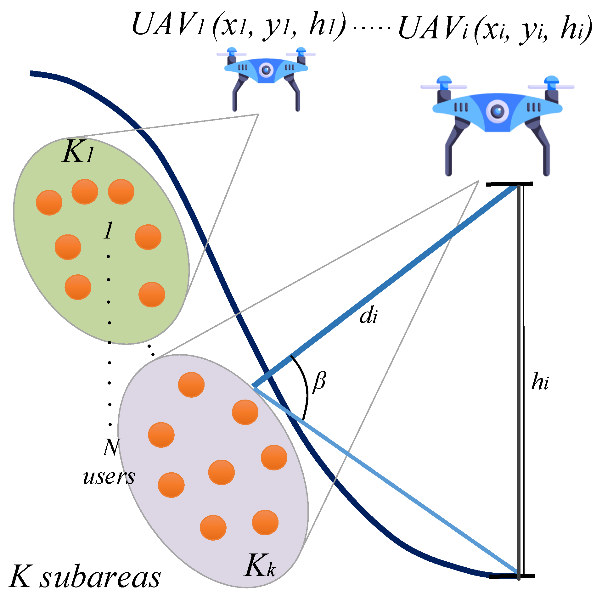
Furthermore, the optimal UAV placement must consider aspects such as the number of ground users, the coverage area, technical wireless parameters, and the channel model between UAV and ground users. The channel model used for communications between UAVs and ground users evaluates the existence of a line of sight (LoS), which means favorable conditions for the signal at the receiver, in addition to assessing non-on line-of-sight (NLoS) scenarios, where the signals arrive by reflections and refractions. Hence, the path loss models depend on the distance between the UAV and the users and the angle they form.

Typically, ground users are modeled on a horizontal plane with uniform height, as in [12]. However, in real-world scenarios, particularly in mountainous regions such as the Andean regions, where cities like Quito are located, the assumption of 2D users does not hold. Irregular topographies with steep slopes and significant elevation differences between populated areas characterize these regions. Residents often live at various heights relative to the city center, directly impacting signal propagation and LoS conditions. Incorporating 3D user models enables a more accurate representation of spatial relationships between UAVs and ground users, especially in regions where vertical variability is not negligible but central to network planning and performance.

Traditional approaches often assume a truncated Gaussian distribution centered around a hotspot. Transitioning from a 2D to a 3D user distribution requires mathematical derivations to generalize the user location model and incorporate height variability. In addition, to represent real scenarios, we consider multiple types of spatial distribution for users, including Gaussian, exponential, and uniform truncated distributions.

Our proposal introduces a complete 3D optimization framework that minimizes the total transmit power of UAVs while guaranteeing a minimum data rate for users at varying altitudes. We incorporate a probabilistic LoS/NLOS channel model based on [13], which accounts for environmental characteristics such as suburban, urban, and dense urban settings. To solve the optimization problem, we implemented the particle swarm optimization evolution (PSO-E) algorithm. PSO-E improves the standard PSO by including adaptive mechanisms and convergence enhancements, making it well suited for complex multidimensional optimization tasks such as the placement of UAVs under realistic communication constraints.

In summary, this work presents the following contributions.

• Optimization of UAV placement by minimizing transmission power while ensuring a guaranteed data rate for ground users;
• Generalization of the traditional 2D user model to a 3D scenario through mathematical derivations, considering user positions relative to UAVs at varying altitudes and addressing practical challenges not captured in existing studies;
• Modeling of ground users considering varying altitudes in suburban, urban, and dense urban environments;
• Analysis of the effect of the user distribution, such as truncated exponential, truncated Gaussian, and uniform distributions within the cell, on transmission power minimization.

Although our work does not propose a new optimization algorithm, we evaluated various heuristic approaches (GA and PSO-E) to solve the complex 3D UAV placement problem under realistic spatial and environmental constraints. Among them, PSO-E was selected for its superior performance in terms of convergence stability, scalability, and computational efficiency. This choice is justified by the need to address a high-dimensional optimization space involving user altitude variability, heterogeneous spatial distributions, and environment-specific LoS/NLoS channel modeling.

The remainder of this paper is organized as follows. Section 2 covers the related work, Section 3 presents the system model, Section 4 outlines the configuration of the system model, Section 5 discusses the results, and Section 6 concludes the paper.

2. Related Work

Optimization of UAV placement has been investigated due to its importance in 5G cellular networks and beyond [14]. This section analyzes papers focused on (i) optimizing UAV placement by maximizing the data rate between UAVs and ground users, (ii) maximizing coverage service, and (iii) minimizing UAV power transmission.

Data rate maximization has been addressed in different works. For example, Chen et al. [15] analyzed the optimal placement of UAVs as repeaters, with a focus on link reliability, evaluating power loss, bit error rate (BER), and outage probability in realistic channel models and comparing amplify, forward-decode, and forward protocols. In addition, Singh et al. [16] studied a cooperative network with multiple UAVs as relays, proposing selection and positioning strategies over the harmonic mean and the best downlink SNR and solving a throughput optimization problem with 3D constraints. Gou et al. [17] addressed the 3D optimization of the position of a UAV acting as a base station by maximizing the data rate for uplink and downlink for ground users. They considered fairness in communication by dividing the optimization problem horizontally and in terms of height. Other researchers, sucha as Wang et al. [18] have operated with multiple UAVs, considering the statistical modeling of users to maximize network performance.

The optimization of UAV coverage has been addressed in various studies. For example, Zhang et al. [19] considered minimizing the number of UAVs that act as base stations in the IoT service area of users. Ma et al. [20] focused on optimizing the coverage of a UAV by considering a channel model for LoS and NLoS links using the Taguchi method. Furthermore, Arribas et al. [21] and Zeng et al. [22] explored both the maximization of coverage and the minimization of energy consumption. The former analyzed relay networks with interference between drones, while the latter provided post-disaster communication in remote areas. Moon et al. [23] proposed an optimal UAV deployment that prioritizes ground users to maximize coverage and analyzed various urban environments.

Several proposals have addressed transmission power optimization, such that by Wei et al. [24], which optimizes the position of UAVs in millimeter wave applications and acts as an aerial base station, providing service to heterogeneous IoT networks. Wu et al. [25] optimized the placement of UAVs and the allocation of power for emergency rescue communications while ensuring the required quality of service. Furthermore, Mozaffari et al. [26] optimized UAV optimizations that minimize UAV power transmission, guaranteeing user data rate requirements.

Similarly, Shakhatreh et al. [27] explored the deployment of UAVs for mm wave communication networks, reducing the optimized power efficiency and network coverage while optimizing the position of the UAV. A single-UAV scenario was analyzed using the Particle Swarm Optimization (PSO) algorithm and a machine learning algorithm to cluster multi-UAV networks. The research showed the importance of UAV altitude, LOS conditions, and energy consumption in optimizing operational costs. Meanwhile, Chen et al. [28] focused on the optimal placement of a UAV for relaying, considering the power loss, outage probability, and bit error rate to determine the best altitude. The study also analyzed the 3D position of a remote station, which served as an information source for the user on the ground.

Zheng et al. [29] used a geometric approach to ensure LOS connectivity in urban environments by proposing a geography-sensitive UAV placement strategy. They proposed an algorithm for optimal placement of UAVs using bounded 2D users in real urban environments, improving relaying and power transmission, minimizing path loss, and ensuring connections.

Unlike previous research using the Air-to-Ground (A2G) channel model, assuming that the ground users were on a 2D surface, this paper considers real scenarios where the users are in 3D. Different probability distributions model their positions to analyze their behavior and impact on minimizing the transmission power of the UAV while ensuring a guaranteed data rate for ground users, as shown in

Table 1. Summary of articles that optimize UAV positioning considering the distribution and position of users.

Study	2D Users	3D Users	User Distribution
Premkumar et al. (2025) [30]	✓	–	Not specified
Zamani et al. (2020) [31]	✓	–	Not specified
Han et al. (2023) [32]	✓	–	Uniform, Gaussian
Ahmad et al. (2022) [33]	✓	–	Uniform
Moon et al. (2022) [23]	✓	–	Uniform
Chuan et al. (2019) [34]	✓	–	Arbitrarily
Our Work	✓	✓	Uniform, Gaussian, Exponential

.

3. System Model

Figure 1 shows a geographical area with uneven terrain and hills, divided into $K=1,\dots ,k$ subareas, where N is the total of 3D ground users distributed according to an arbitrary distribution. UAVs act as base stations, with each ${\mathrm{UAV}}_i$ serving a specific subarea (K) positioned at $(x_i,y_i,h_i)$ in Cartesian coordinates. Each index (i) refers to a specific UAV that serves a unique subarea defined as $[X_{K,i},X_{K,i+1}]\times [Y_{K,i},Y_{K,i+1}]\times [Z_{K,i},Z_{K,i+1}]\subset \mathbb{R}$, forming a 3D coverage region.

We consider a downlink scenario in which UAVs transmit data using the frequency division multiple access (FDMA) technique, with each ground user assigned a dedicated communication channel. The model assumes that the UAVs’ total power and available bandwidth are sufficient to meet the data requirements of all users. In addition, it transmits over different frequency bands without interference and assumes that no other wireless communications are present. Each ${\mathrm{UAV}}_i$ covers a specific subarea ($K_i$) with predetermined cell boundaries.

3.1. Air-to-Ground Channel Model

The communication system employs an A2G channel model that accounts for both LoS and NLoS links in large-scale applications. An LoS link describes a direct line of sight between the UAV and ground users. In contrast, an NLoS link occurs when the direct path is blocked by obstacles (e.g., terrain or buildings), leading to alternative propagation mechanisms, such as reflection, diffraction, or scattering. The path loss for LoS and NLoS is denoted by $L_i(x,y,z)$, and the links between ${\mathrm{UAV}}_i$ and the ground users are expressed as follows [13]:

$$L_i(x,y,z)=\left\{\begin{array}{cc}{\left({\displaystyle \frac{4\pi f_c}{c}}\right)}^2{\left|d_i(x,y,z)\right|}^{\alpha }{\mu }_{\mathrm{LoS}},\hfill & \mathrm{LoS}\mathrm{link},\hfill \\ {\left({\displaystyle \frac{4\pi f_c}{c}}\right)}^2{\left|d_i(x,y,z)\right|}^{\alpha }{\mu }_{\mathrm{NLoS}},\hfill & \mathrm{NLoS}\mathrm{link},\hfill \end{array}\right.$$

(1)

where $\left|d_i(x,y,z)\right|$ is the distance between ${\mathrm{UAV}}_i$ and ground users, $\alpha$ is the path loss exponent, $f_c$ is the carrier frequency, c is the speed of light, and ${\mu }_{\mathrm{LoS}}$ and ${\mu }_{\mathrm{NLoS}}$ are additional path loss factors for LoS and NLoS links, respectively. Environmental factors such as the concentration and height of the building, classified as suburban, urban, or dense urban, and the relative positions of users and UAVs influence the LoS link. The following expression models this probability ($P_{LoS}$), as defined in [13] and Equation (2):

$$P_{LoS}={\displaystyle \frac{1}{1+aexp(-b[\theta -a\left]\right)}},$$

(2)

where a and b are constants depending on the environment (suburban, urban, or dense urban) and $\theta$ is the elevation angle given by [26]. Based on Figure 2, the following parameters are defined:

$$\theta ={\displaystyle \frac{180}{\pi }}{sin}^{-1}\left({\displaystyle \frac{h_i}{d(x_i,y_i)}}\right),$$

(3)

Equation (3) applies to 2D ground users, but the angle ($\theta$) differs when the users are at varying heights. $\beta$ defines the angle between 3D ground users $(x,y,z)$ and $UA{V}_i$.

Proposition 1. 

β angle for ground users in 3D and $UA{V}_i$.

$$\beta ={\displaystyle \frac{180}{\pi }}{sin}^{-1}\left({\displaystyle \frac{d_x(x,y)·h_i}{d_1(x,y,z)·d_i(x,y,z)}}\right).$$

(4)

where:

$$d_x(x,y)=\sqrt{{(x_i-x)}^2+{(y_i-y)}^2},$$

(5)

$$d_i(x,y,z)=\sqrt{{(x_i-x)}^2+{(y_i-y)}^2+{(h_i-z)}^2}$$

(6)

$$d_1(x,y,z)=\sqrt{{(x_i-x)}^2+{(y_i-y)}^2+z^2}$$

(7)

Proof of Proposition 1. 

See Appendix A.    □

Thus, the probabilities for LoS and NLoS on the $\beta$ angle are expressed as follows:

$$\left\{\begin{array}{c}{P}_{LoS}={\displaystyle \frac{1}{1+aexp(-b[\beta -c\left]\right)}},\hfill \\ P_{NLoS}=1-P_{LoS}.\hfill \end{array}\right.$$

(8)

According to (1) and (8), the average path loss for the A2G channel model is expressed as follows:

$$\begin{array}{cc}\hfill \overline{L_i}(x,y,z)=& P_{LoS}{\left({\displaystyle \frac{4\pi f_c}{c}}\right)}^2{\left|d_i(x,y,z)\right|}^{\alpha }{\mu }_{\mathrm{LoS}}\hfill \\ \hfill & + P_{NLoS}{\left({\displaystyle \frac{4\pi f_c}{c}}\right)}^2{\left|d_i(x,y,z)\right|}^{\alpha }{\mu }_{\mathrm{NLoS}}.\hfill \end{array}$$

(9)

3.2. Problem Formulation

Given the spatial configuration of ${\mathrm{UAV}}_i$ and ground users located at $(x,y,z)$ with varying heights, the achievable data rate ($R_i$) can be determined as [13] Equation (10):

$$R_i(x,y,z)={\displaystyle \frac{B_i}{M_i}}·{log}_2\left(1+{\displaystyle \frac{P_i(x,y,z)}{N_0·\overline{L_i}(x,y,z)}}\right),$$

(10)

where $B_i$ represents the total available bandwidth for the ${\mathrm{UAV}}_i$; $M_i$ is the number of users served by ${\mathrm{UAV}}_i$; $P_i(x,y,z)$ is the power transmission of ${\mathrm{UAV}}_i$ to a 3D user; $\overline{L_i}(x,y,z)$ is the average path loss between ${\mathrm{UAV}}_i$ and the user; and, finally, $N_0$ is the additive white Gaussian noise power. Here, $M_i$ depends on the number of users within the cell boundaries of ${\mathrm{UAV}}_i$, which is expressed as follows:

$$M_i=N{\int \int \int }_{C_i}f(x,y,z)dxdydz,$$

(11)

where $C_i$ defines the cell boundary covered by ${\mathrm{UAV}}_i$. The number of users covered by each ${\mathrm{UAV}}_i$ depends on the distribution of users, cell boundaries, and the position of ${\mathrm{UAV}}_i$.

According to (10), the minimum transmit power required to meet the rate requirement, denoted by $\gamma$, for each user is expressed as follows:

$$P_{i,min}(x,y,z)=\left(2^{{\displaystyle \frac{\gamma ·M_i}{B_i}}}-1\right)N_0·\overline{L_i}(x,y,z),$$

(12)

where $R_i(x,y,z)\ge \gamma$. As the number of users increases, the bandwidth per user decreases, which requires higher transmit power to maintain the desired rate. Thus, average total transmit power for the full system is expressed as follows:

$$P_t=\sum _{i=1}^K{\int \int \int }_{C_i}{P}_{i,min}(x,y,z)f(x,y,z)dxdydz,$$

(13)

where $f(x,y,z)$ is the probability distribution of the users. The optimization objective minimizes the total average transmission power of the system (Equation (12) in Equation (13)). The aim is to optimize the locations of ${\mathrm{UAV}}_i$, minimizing the transmission power while ensuring the data rate requirements for all 3D ground users. This results in the following optimization problem.

$$\begin{array}{cc}\hfill \underset{x_i,y_i,z_i}{min}{P}_t=& \sum _{i=1}^K{\int \int \int }_{C_i}\left(2^{{\displaystyle \frac{\gamma ·M_i}{B_i}}}-1\right)N_0·\hfill \\ \hfill & \overline{L_i}(x,y,z)·f(x,y,z)dxdydz,\hfill \end{array}$$

(14)

$$\begin{array}{c}\hfill \mathrm{s}.\mathrm{t}.\end{array}$$

(15)

$$\begin{array}{cc}\hfill C1:& \sum _{i=1}^K{P}_i⩽P,\hfill \end{array}$$

(16)

$$\begin{array}{cc}\hfill C2:& x_i>0,y_i>0,z_i>0,iϵ\left\{\begin{array}{c}1....K\end{array}\right\},\hfill \end{array}$$

(17)

$$\begin{array}{cc}\hfill C3:& x>0,y>0,z>0,iϵ\left\{\begin{array}{c}1....N\end{array}\right\},\hfill \end{array}$$

(18)

where $C1$ indicates that P is the total available power of the system; $C2$ ensures that the ${\mathrm{x}}_i$, ${\mathrm{y}}_i$, and ${\mathrm{z}}_i$ coordinates of ${\mathrm{UAV}}_i$ are positive; and, finally, $C3$ guarantees positive 3D locations of users.

4. System Model Configuration

Three scenarios were analyzed, each defined by a different probability distribution: (i) truncated Gaussian, (ii) truncated exponential, and (iii) truncated uniform distributions. The users are located within a cell with dimensions of $\left[D{x}_i,D{x}_s\right]\times \left[D{y}_i,D{y}_s\right]\times \left[D{z}_i,D{z}_s\right]$, where $D{x}_i=D{y}_i=D{z}_i=\left\{0\right\}$, $D{x}_s=D{y}_s=\left\{500\right\}$ m, and $D{z}_s=\{50,100,150\}$ m [35]. The values of $D{z}_s=\{50,100,150\}$ represent discrete user altitudes along geographical slopes, modeling typical elevation levels of terrain such as valley floors, mid-slopes, and hilltops.

The truncated Gaussian distribution models a scenario with a hotspot in the center of the cell, with user population density decreasing toward the periphery. This distribution is expressed as follows.

$$\begin{array}{cc}\hfill f(x,y,z)=& {\displaystyle \frac{1}{G}}exp\left(-{\displaystyle \frac{{(x-{\mu }_x)}^2}{2{\sigma }_x^2}}\right)exp\left(-{\displaystyle \frac{{(y-{\mu }_y)}^2}{2{\sigma }_y^2}}\right)\hfill \\ \hfill & exp\left(-{\displaystyle \frac{{(z-{\mu }_z)}^2}{2{\sigma }_z^2}}\right).\hfill \end{array}$$

(19)

The constant (G) is defined as follows:

$$\begin{array}{cc}\hfill G=& 2\sqrt{2}{\pi }^{3/2}\sqrt{{\sigma }_x^2{\sigma }_y^2{\sigma }_z^2}\hfill \\ \hfill & \left({\displaystyle \frac{1}{2}}\left(-Erf\left({\displaystyle \frac{D_{x\mathrm{i}}-{\mu }_x}{\sqrt{2}{\sigma }_x}}\right)+Erf\left({\displaystyle \frac{D_{x\mathrm{s}}-{\mu }_x}{\sqrt{2}{\sigma }_x}}\right)\right)\right)\hfill \\ \hfill & \left({\displaystyle \frac{1}{2}}\left(-Erf\left({\displaystyle \frac{D_{y\mathrm{i}}-{\mu }_y}{\sqrt{2}{\sigma }_y}}\right)+Erf\left({\displaystyle \frac{D_{y\mathrm{s}}-{\mu }_y}{\sqrt{2}{\sigma }_y}}\right)\right)\right)\hfill \\ \hfill & \left({\displaystyle \frac{1}{2}}\left(-Erf\left({\displaystyle \frac{D_{z\mathrm{i}}-{\mu }_z}{\sqrt{2}{\sigma }_z}}\right)+Erf\left({\displaystyle \frac{D_{z\mathrm{s}}-{\mu }_z}{\sqrt{2}{\sigma }_z}}\right)\right)\right),\hfill \end{array}$$

(20)

where the ${\mu }_x$, ${\mu }_y$, and ${\mu }_z$ parameters represent the means of the Gaussian distributions, $Erf\left(w\right)={\displaystyle \frac{2}{\sqrt{\pi }}}{\int }_0^w{e}^{-t^2}dt$, and the user population density is influenced by the standard deviations of ${\sigma }_x$, ${\sigma }_y$, and ${\sigma }_z$. Specifically, the densities along each axis are given by ${\rho }_x^{\mathit{G}}={\displaystyle \frac{1}{{\sigma }_x}}$, ${\rho }_y^{\mathit{G}}={\displaystyle \frac{1}{{\sigma }_y}}$, and ${\rho }_z^{\mathit{G}}={\displaystyle \frac{1}{{\sigma }_z}}$.

The truncated exponential distribution models the user concentration predominantly on one side of the cell and is expressed as follows:

$$f(x,y,z)={\displaystyle \frac{1}{H}}{e}^{-{\lambda }_{x}x-{\lambda }_{y}y-{\lambda }_{z}z},$$

(21)

where the normalization constant (H) is expressed as follows:

$$\begin{array}{cc}\hfill H=& \left({\displaystyle \frac{1}{{\lambda }_x}}\left(e^{-{\lambda }_x{D}_{x\mathrm{i}}}-e^{-{\lambda }_x{D}_{x\mathrm{s}}}\right)\right)\left({\displaystyle \frac{1}{{\lambda }_y}}\left(e^{-{\lambda }_y{D}_{y\mathrm{i}}}-e^{-{\lambda }_y{D}_{y\mathrm{s}}}\right)\right)\hfill \\ \hfill & \left({\displaystyle \frac{1}{{\lambda }_z}}\left(e^{-{\lambda }_z{D}_{z\mathrm{i}}}-e^{-{\lambda }_z{D}_{z\mathrm{s}}}\right)\right)\hfill \end{array}$$

(22)

Here, the $\lambda$ parameter defines the user population density, and its reciprocal corresponds to the standard deviation along each axis: ${\rho }_x^{\mathit{E}}={\displaystyle \frac{1}{{\lambda }_x}}$, ${\rho }_y^{\mathit{E}}={\displaystyle \frac{1}{{\lambda }_y}}$, and ${\rho }_z^{\mathit{E}}={\displaystyle \frac{1}{{\lambda }_z}}$.

The uniform distribution assumes that users are evenly spread across the entire cell is expressed as follows:

$$f(x,y,z)={\displaystyle \frac{1}{(D_{xs}-D_{xi})(D_{ys}-D_{yi})(D_{zs}-D_{zi})}}.$$

(23)

In each scenario, simulations were conducted for three distinct environments: (i) suburban, (ii) urban, and (iii) dense urban environments.

Table 2. Constants and parameters of different environments.

Parameter	Environment
	Suburban	Urban	Dense Urban
a	4.88	9.61	12.08
b	0.43	0.16	0.11
${\eta }_{LoS}$	0.1 dB	1 dB	1.6 dB
${\eta }_{NLoS}$	21 dB	20 dB	23 dB

shows the radio frequency parameters for LoS and NLoS connections and the environment constants (a and b), and

Table 3. Simulation parameters.

Parameter	Description	Value
$f_c$	Carrier Frequency	2.5 GHz
$\gamma$	Data rate required by users	10 Mbps
N	Number of ground users	50
c	Speed of light	3 × 108 m/s
$N_0$	Noise power	2.0019 × 10−12 W/Hz
B	Bandwidth for each UAV	50 MHz
$\alpha$	The path loss exponent	2

presents the simulation parameters of the system, including the operating frequency, the number of users, and noise power, among others, as used in [36]. All simulations were carried out using Wolfram Mathematica 12.1. computational software.

Table 4. PSO-E parameters.

Parameter	Description	Value
p	Population	2000
$iterations$	Number of iterations	5
$\tau$	Learning parameter	1
${\tau }_1$	Learning parameter	0.2
$iner1$	Inertia weight	0.5
$mem1$	Memory Value	2
$coop1$	Cooperation value	3
$pert1$	Perturbation value	0.1
$Xmin$	Initial value of x-axis	5 [m]
$Xmax$	Final value of x-axis	450 [m]
$Ymin$	Initial value of y-axis	5 [m]
$Ymax$	Final value of y-axis	450 [m]
$hmin$	Initial value of altitude	5 [m]
$hmax$	Final value of altitude	200 [m]

shows the parameters used in the PSO-E algorithm to find the system solution; such as the size of the population, the number of iterations; and parameters such as inertia, memory, cooperation, and learning, as described in [37]. A large population size of 2000 particles was selected to enhance the algorithm’s exploration capability. The number of iterations was limited to 5, which allows us to reach the result. The learning parameters ($\tau$ and ${\tau }_1$) control the adaptability of the particles during the optimization process. The inertia weight ($iner1$) influences the momentum of each particle. At the same time, the values of memory ($mem1$) and cooperation ($coop1$) regulate how much a particle relies on its own experience versus the best known position of the group. Furthermore, a perturbation factor ($pert1$) introduces stochastic variations to avoid premature convergence.

Problem Complexity

The UAV optimization problem is formulated as a Mixed-Integer Nonlinear Programming (MINLP) model, where the goal is to minimize transmission power while ensuring a required data rate for ground users at different altitudes. Due to the non-linearity of the objective function, influenced by the channel model and user distribution, obtaining an exact solution is intractable [38]. Heuristic methods are used to achieve a computationally feasible solution [39]. In this work, we employ the PSO-E algorithm (Algorithm 1), originally proposed in [37], which integrates evolutionary strategies into the classical PSO to enhance exploration and avoid premature convergence. Unlike the standard PSO, PSO-E incorporates mutation operators and natural selection mechanisms that allow particles to diversify their search behavior while preserving the most promising solutions. These features have demonstrated robustness in solving complex optimization problems such as [37]. Although PSO-E does not theoretically guarantee convergence to the global optimum in every execution, its convergence behavior was analyzed in detail in [37], where the authors described how evolutionary operators improve the algorithm’s performance with respect to solution quality and stability.

The PSO-E Algorithm 1 extends the standard PSO by incorporating mechanisms of adaptive inertia, memory, cooperation, and a perturbation phase to improve the precision of the solution and escape local optima. The algorithm starts by defining the objective function to minimize (Equation (14)), initializing the parameters of the swarm, such as population size, the number of iterations, and learning factors for personal and global experiences. Each particle in the swarm is randomly placed within a 3D bounded space defined by the (x,y,z) coordinates, and its fitness is evaluated according to the objective function (lines 11 to 20). Each particle retains its best position so far (xpbest) and its corresponding fitness value (fpbest). The best solution among all particles is stored as the best global solution(xgbest) with its fitness (fgbest) (lines 21 to 24). During each iteration, the particles update their velocities based on a weighted combination of inertia, memory (which reflects the influence of the best position of the individual), and cooperation (which reflects the influence of the best global position). These components are slightly perturbed in each iteration using the $\tau$ parameter, allowing the swarm to balance exploration and exploitation dynamically. The updated velocities are then used to compute new positions, which are constrained to stay within predefined boundaries. After evaluating the new positions, each particle updates its personal best if a better fitness is found. Similarly, the best global solution is updated when any particle finds a superior solution. An additional enhancement of PSO-E involves perturbing the global best position using a separate parameter ($\tau 1$); if the perturbed candidate improves the objective value, it replaces the current global best. This mechanism enhances the algorithm’s ability to escape local minima. The process continues until a maximum number of iterations is reached. At this point, the best global position is returned as the final solution.

Algorithm 1 PSO-E Algorithm

1: function  PSO-E 2:       objective ← Equation (14) 3:       iterations $\leftarrow \#iterations$ 4:       p $\leftarrow \#population$                                                                                    ▹ Population size 5:       $\tau \leftarrow c\text{-}init$                                                    ▹ Learning parameter for local best pos. 6:       ${\tau }_1\leftarrow c\text{-}init$                                                ▹ Learning parameter for global best pos. 7:       iner1 ← InertiaValue                                                                           ▹ Inertia weight 8:       mem1 ← MemoryValue                                                                               ▹ Memory 9:       coop1 ← CoopValue                                                                              ▹ Cooperation 10:     pert1 ← PerValue                                                                                   ▹ Perturbation 11:     $D_{min}\leftarrow [X_{min},Y_{min},h_{min}]$ 12:     $D_{max}\leftarrow [X_{max},Y_{max},h_{max}]$ 13:     $D\leftarrow \mathrm{length}\left(D_{min}\right)$ 14:     $x\leftarrow \mathrm{zeros}\left[\mathrm{Length}\right(p),D]$ 15:     $v\leftarrow \mathrm{zeros}\left[\mathrm{Length}\right(p),D]$ 16:     $fitness\leftarrow \mathrm{zeros}\left[\mathrm{Length}\right(p),1]$ 17:     for $i\leftarrow 1$ to D do 18:           $x(:,i)\leftarrow (D_{max}\left(i\right)-D_{min}\left(i\right))\ast \mathrm{rand}(p,1)+D_{min}\left(i\right)$ 19:     end for 20:     $fitness\leftarrow \mathrm{objective}\left(x\right)$ 21:     $[fgbest,indgbest]\leftarrow \min \left(fitness\right)$ 22:     $xgbest\leftarrow x(indgbest,:)$ 23:     $fpbest\leftarrow fitness$ 24:     $xpbest\leftarrow x$ 25:     for $count\leftarrow 1$ to iterations do 26:           $\mathrm{OF}\left(count\right)\leftarrow fgbest$ 27:           $iner\leftarrow iner1+\tau ·\mathrm{rand}(p,D)$ 28:           $iner(iner>1)\leftarrow 1$ 29:           $iner(iner<0)\leftarrow 0$ 30:           $mem\leftarrow mem1+\tau ·\mathrm{rand}(p,D)$ 31:           $mem(mem>1)\leftarrow 1$ 32:           $mem(mem<0)\leftarrow 0$ 33:           $coop\leftarrow coop1+\tau ·\mathrm{rand}(p,D)$ 34:           $coop(coop>1)\leftarrow 1$ 35:           $coop(coop<0)\leftarrow 0$ 36:           $v\leftarrow iner·v+mem·(xpbest-x)+coop·(xgbest-x)$ 37:           $x\leftarrow x+v$ 38:           for $i\leftarrow 1$ to D do 39:                 $x(x(:,i)<D_{min}\left(i\right),i)\leftarrow D_{min}\left(i\right)$ 40:                 $x(x(:,i)>D_{max}\left(i\right),i)\leftarrow D_{max}\left(i\right)$ 41:         end for 42:         $fitness\leftarrow \mathrm{objective}\left(x\right)$ 43:         $idx\leftarrow \mathrm{find}(fitness<fpbest)$ 44:         $xpbest(idx,:)\leftarrow x(idx,:)$ 45:         $fpbest\left(idx\right)\leftarrow fitness\left(idx\right)$ 46:         $[fgbest,indgbest]\leftarrow min\left(fitness\right)$ 47:         $xgbest\leftarrow x(indgbest,:)$ 48:         $pert\leftarrow pert1+{\tau }_1·\mathrm{rand}(1,\mathrm{length}\left(xgbest\right))$ 49:         $pert(pert>1)\leftarrow 1$ 50:         $pert(pert<0)\leftarrow 0$ 51:         $aux\leftarrow xgbest+pert$ 52:         if $fgbest>\mathrm{objective}\left(aux\right)$ then 53:             $xgbest\leftarrow aux$ 54:             $fgbest\leftarrow \mathrm{objective}\left(aux\right)$ 55:         end if 56:     end for 57: end function

5. Analysis of Results and Discussion

This section presents the results of the optimal placement of 3D UAV-enabled communication scenarios evaluated using the PSO-E algorithm (Algorithm 1), aimed at minimizing transmission power while ensuring the required data rate for ground users at different altitudes.

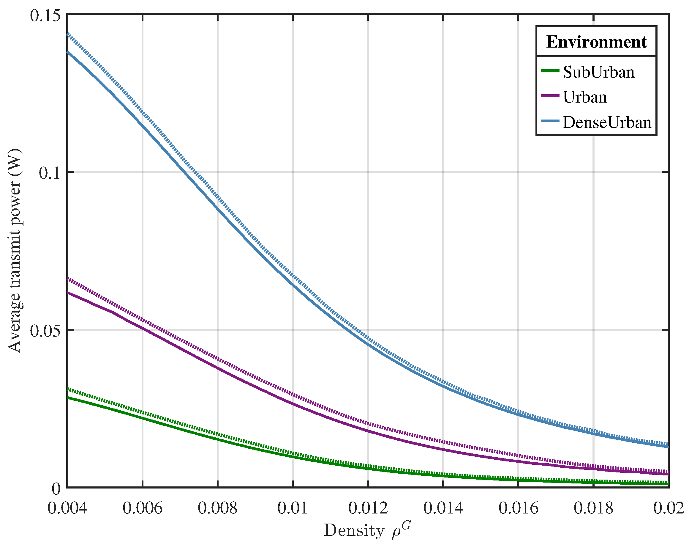
To validate the effectiveness of the proposed approach, we compare PSO-E with a classical Genetic Algorithm (GA) previously shown to achieve near-optimal solutions in similar problems [40]. Figure 3 illustrates the average transmission power of UAVs as a function of the density of ground users (${\rho }^{\mathrm{G}}$) in three different environments—suburban, urban, and dense urban—with a cell size of ($D_x=500,D_y=500,D_z=100$). The solid lines represent the results obtained using PSO-E, while the dotted lines correspond to GA. As shown, the two algorithms achieve comparable performance in terms of solution quality.

Table 5. Comparison of computational efforts between PSO-E and GAs. “Red.” stands for reduction.

Population	Time in Seconds		Memory in Use (kilobytes)		Value [W]		Time Red. (%)	Memory Red. (%)
	PSO-E	Genetic	PSO-E	Genetic	PSO-E	Genetic
100	197.1	344.8	332.21	476.85	0.006	0.010	42.83	30.33
150	267.7	762.93	577.17	812.71	0.005	0.008	64.7	28.98
200	342.5	919.3	731.64	974.61	0.006	0.006	62.75	24.89

compares computational efforts between PSO-E and genetic algorithms in urban scenarios. The results confirm that PSO-E reached solutions, on average, in 197.1 s for 100 points of the population, while GA required 344.8 s, representing a reduction of 42.84% in computation time. As the population size increases to 150 and 200 points, the time savings achieved by PSO-E exceed 60%, highlighting its scalability and computational efficiency in more demanding scenarios. These results confirm that PSO-E maintains comparable solution quality while significantly reducing execution time compared to GA.

To promote reproducibility, the implementation code used in this study, including the PSO-E algorithm and simulation framework, will be made available via a GitHub repository. https://github.com/Jcarvajal01/Optimization-of-Transmission-Power-in-a-3D-UAV-Enabled-Communication-System- (accessed on 31 May 2025).

The curves in Figure 3 show a similar trend for both algorithms; however, PSO-E demonstrates a closer approximation in minimizing the transmit power of the UAV. Therefore, the PSO-E algorithm is used in subsequent simulations. In addition, the dense urban environment consumes nearly twice the power of the urban environment, showing the highest average transmit power, while the suburban environment requires the least power.

Figure 4 shows that the transmit power vs. the population density of the users of both the exponential and the Gaussian distributions in urban environments, denoted by ${\rho }^E$ and ${\rho }^G$, respectively. For the sake of simple notation, we set ${\rho }^E={\rho }^G={\rho }^{G,E}$. The solid line represents a truncated Gaussian distribution with a mean of ${\mu }_x=250, {\mu }_y=250$ and ${\mu }_z=25, 50, 75$ equal to the mean of the cell and a standard deviation ($\sigma$). The dotted line corresponds to an exponential distribution, where the standard deviation is the inverse of $\lambda$. The dotted markers indicate a uniform distribution, where users are evenly spread across the cell.

Moreover, Figure 4 shows that the transmit power decreases as the density of the user population increases at all altitudes, with the highest power required at 0 m and the lowest at 150 m. The inset zooms in on the region with high user population density, highlighting the trend more clearly. The required UAV transmit power for Gaussian and exponential distributions at user altitudes of 100 and 150 m is approximately equal. However, a noticeable difference emerges as the user population density increases, with the Gaussian distribution requiring less power. In contrast, the opposite behavior is observed for low densities at lower user altitudes. There is a clear difference in power between the Gaussian and exponential distributions, but as user population density increases, the required power for both distributions converges. Additionally, the uniform distribution consistently demands the highest power compared to the other distributions across all scenarios.

Figure 5 combines multiple curves illustrating the relationship between ${\mathrm{UAV}}_i$ altitude and average transmit power in different environments and distributions. Figure 5a shows that the exponential truncated distribution requires more power than urban and suburban environments. Figure 5b highlights that in the urban environment, the truncated Gaussian distribution demands nearly twice the power of the Gaussian distribution. Figure 5c reveals that the uniform distribution in dense urban environments requires more power than in suburban and urban settings for the same distribution. Generally, the urban environment requires less power than other environments in all distributions.

The analysis considered the UAV transmit power required to serve ground users at heights of 0, 50, 100, and 150 m. Figure 5g–i indicate that the optimal heights of ${\mathrm{UAV}}_i$ are almost independent of the distribution used in the suburban environment. However, the optimal heights of the UAV vary with the distribution in urban and dense urban environments. The uniform distribution requires the highest UAV altitude, while the exponential distribution demands the lowest.

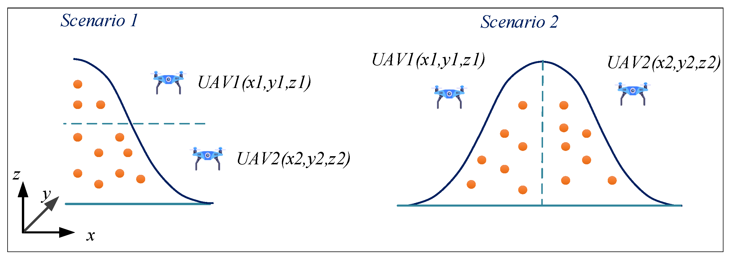
Figure 6 illustrates two simulation scenarios, each implemented with two UAVs. The first scenario divides the area vertically, with a service area measuring 500 × 500 m along the x and y axes. For the z-axis, ground users are simulated at two different heights: 100 and 200 m. Each UAV serves a 500 × 500 × 50 m cell for the first height, extending to 100 m.

In the second scenario, the system models a complete elevation with one UAV on each side, dividing the area horizontally. The dimensions are 1000 × 500 m along the x and y axes, with the same height levels as in the first scenario. The x-axis is divided into two sections, with each cell measuring 500 × 500 × 100 m for the first height and extending to 200 m for the second height.

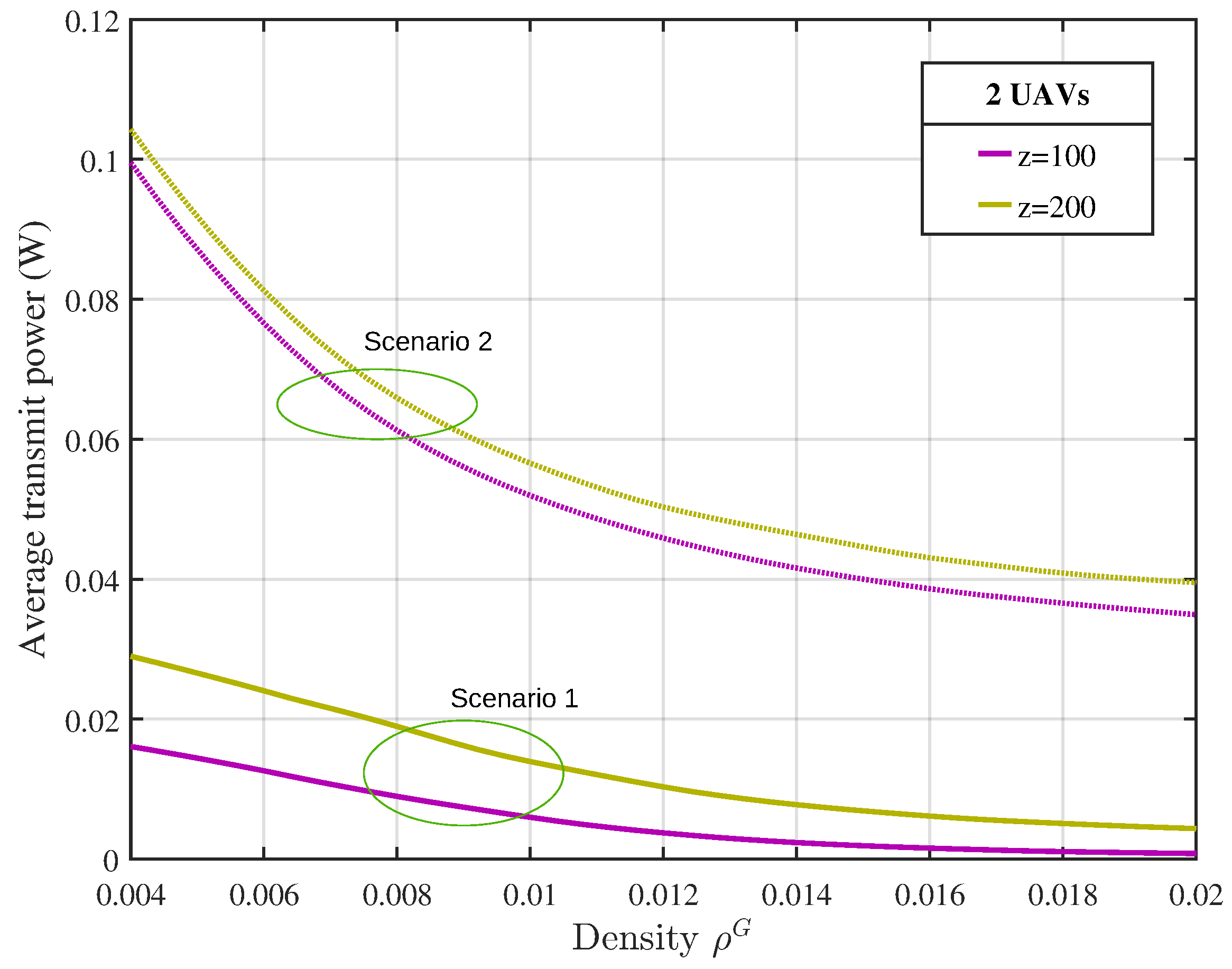
Figure 7 presents the simulation results of the scenarios in Figure 6, showing the average transmission power versus the density of the user population (${\rho }^{\mathrm{G}}$) using a truncated Gaussian distribution. The results differ between the scenarios, with the transmission power required in the first scenario being approximately one-third that in the second. In the first scenario, at a height of 200 [m] and a low density of the user population, the power consumption is more significant than 100 [m], and the power difference between heights of z = 100 and z = 200 [m] does not remain constant as the power decreases. In other words, users are not concentrated in the hotspot but spread across the cell. However, power transmission becomes more balanced as the density of the user population increases. In the second scenario, the required power is higher than that of a single-UAV deployment. However, the combined power of the two UAVs is not double that of a single UAV at z = 100 [m]. At z = 200 [m], the power difference remains minimal and consistent between the different densities of users.

6. Conclusions

This research presents a mathematical model (framework) to determine the optimal placement of UAVs serving ground users with varying altitudes. It addresses scenarios with complex terrain, such as in Andean cities. Unlike traditional approaches that assume flat terrain and uniform user height, our model incorporates realistic user distributions and elevation variability.

The proposed framework minimizes the total transmit power while ensuring guaranteed data rate requirements. It integrates a probabilistic LoS/NLoS channel model adapted to different suburban, urban, and dense urban environments and supports several spatial users, including Gaussian, exponential, and uniform truncated distributions.

The results highlight the impact of the user distribution in 3D and the analyzed environment on the total power required by the UAV. In particular, denser urban environments and uniformly distributed users demand significantly more power. The dense urban environment consistently requires approximately 50% of the highest average transmit power for the urban scenario and two orders of magnitude higher (300%) than for the suburban scenario, along with all the variation in the density of the user population. The uniform distribution requires more than 50% additional power compared to the Gaussian distribution and approximately 10% more than the exponential distribution.

Overall, the results show the importance of incorporating 3D user models in different environments and optimization techniques such as the PSO-E algorithm for UAV position optimization.

Future research could investigate the analysis of 3D UAV placement-enabled communications using small-scale channel models in urban settings. This approach would provide a more accurate representation and help us know the impact of a small signal on the optimal position of the UAV.

References

1. Zhu, X. Analysis of military application of UAV swarm technology. In Proceedings of the 2020 3rd International Conference on Unmanned Systems (ICUS), Harbin, China, 27–28 November 2020; pp. 1200–1204. [Google Scholar] [CrossRef]
2. Shakhatreh, H.; Sawalmeh, A.H.; Al-Fuqaha, A.; Dou, Z.; Almaita, E.; Khalil, I.; Othman, N.S.; Khreishah, A.; Guizani, M. Unmanned Aerial Vehicles (UAVs): A Survey on Civil Applications and Key Research Challenges. IEEE Access 2019, 7, 48572–48634. [Google Scholar] [CrossRef]
3. Mozaffari, M.; Saad, W.; Bennis, M.; Debbah, M. Mobile Unmanned Aerial Vehicles (UAVs) for Energy-Efficient Internet of Things Communications. IEEE Trans. Wirel. Commun. 2017, 16, 7574–7589. [Google Scholar] [CrossRef]
4. Li, M.; Hong, Y.; Zeng, C.; Song, Y.; Zhang, X. Investigation on the UAV-To-Satellite Optical Communication Systems. IEEE J. Sel. Areas Commun. 2018, 36, 2128–2138. [Google Scholar] [CrossRef]
5. Mozaffari, M.; Saad, W.; Bennis, M.; Nam, Y.H.; Debbah, M. A Tutorial on UAVs for Wireless Networks: Applications, Challenges, and Open Problems. IEEE Commun. Surv. Tutor. 2019, 21, 2334–2360. [Google Scholar] [CrossRef]
6. Song, Q.; Zeng, Y.; Xu, J.; Jin, S. A survey of prototype and experiment for UAV communications. Sci. China Inf. Sci. 2021, 64, 140301. [Google Scholar] [CrossRef]
7. Baltaci, A.; Dinc, E.; Ozger, M.; Alabbasi, A.; Cavdar, C.; Schupke, D. A Survey of Wireless Networks for Future Aerial Communications (FACOM). IEEE Commun. Surv. Tutor. 2021, 23, 2833–2884. [Google Scholar] [CrossRef]
8. Bekmezci, İ.; Sahingoz, O.K.; Temel, Ş. Flying Ad-Hoc Networks (FANETs): A survey. Ad Hoc Netw. 2013, 11, 1254–1270. [Google Scholar] [CrossRef]
9. Yang, P.; Cao, X.; Yin, C.; Xiao, Z.; Xi, X.; Wu, D. Proactive Drone-Cell Deployment: Overload Relief for a Cellular Network Under Flash Crowd Traffic. IEEE Trans. Intell. Transp. Syst. 2017, 18, 2877–2892. [Google Scholar] [CrossRef]
10. Shabanighazikelayeh, M.; Koyuncu, E. Optimal Placement of UAVs for Minimum Outage Probability. IEEE Trans. Veh. Technol. 2022, 71, 9558–9570. [Google Scholar] [CrossRef]
11. Carvajal-Rodríguez, J.; Guamán, D.S.; Tipantuña, C.; Urquiza, L.F. 3D Placement Optimization in UAV-Enabled Communications: A Systematic Mapping Study. IEEE Open J. Veh. Technol. 2024, 5, 523–559. [Google Scholar] [CrossRef]
12. Gupta, M.; Varma, S. Optimal placement of UAVs of an aerial mesh network in an emergency situation. J. Ambient. Intell. Humaniz. Comput. 2021, 12, 343–358. [Google Scholar] [CrossRef]
13. Al-Hourani, A.; Kandeepan, S.; Lardner, S. Optimal LAP Altitude for Maximum Coverage. IEEE Wirel. Commun. Lett. 2014, 3, 569–572. [Google Scholar] [CrossRef]
14. Elnabty, I.A.; Fahmy, Y.; Kafafy, M. A survey on UAV placement optimization for UAV-assisted communication in 5G and beyond networks. Phys. Commun. 2022, 51, 101564. [Google Scholar] [CrossRef]
15. Gupta, N.; Agarwal, S.; Mishra, D. UAV Deployment for Throughput Maximization in a UAV-Assisted Cellular Communications. In Proceedings of the 2021 IEEE 32nd Annual International Symposium on Personal, Indoor and Mobile Radio Communications (PIMRC), Helsinki, Finland, 13–16 September 2021; pp. 1055–1060. [Google Scholar] [CrossRef]
16. Singh, S.K.; Agrawal, K.; Singh, K.; Li, C.P.; Huang, W.J. On UAV Selection and Position-Based Throughput Maximization in Multi-UAV Relaying Networks. IEEE Access 2020, 8, 144039–144050. [Google Scholar] [CrossRef]
17. Guo, H.; Zou, Y.; Wu, T.; Zhou, F. 3D location optimization for UAV-aided uplink/downlink transmissions. IEEE Trans. Veh. Technol. 2022, 71, 4477–4482. [Google Scholar] [CrossRef]
18. Wang, L.; Zhang, H.; Guo, S.; Yuan, D. 3D UAV Deployment in Multi-UAV Networks With Statistical User Position Information. IEEE Commun. Lett. 2022, 26, 1363–1367. [Google Scholar] [CrossRef]
19. Zhang, C.; Zhang, L.; Zhu, L.; Zhang, T.; Xiao, Z.; Xia, X.G. 3D Deployment of Multiple UAV-Mounted Base Stations for UAV Communications. IEEE Trans. Commun. 2021, 69, 2473–2488. [Google Scholar] [CrossRef]
20. Ma, Z.; Huangfu, W.; Liu, Y. Optimizing 3-D Placement of Multiple UAVs Based on Taguchi’s Method. In Proceedings of the 2020 IEEE Intl Conf on Parallel & Distributed Processing with Applications, Big Data & Cloud Computing, Sustainable Computing & Communications, Social Computing & Networking (ISPA/BDCloud/SocialCom/SustainCom), Exeter, UK, 17–19 December 2020; pp. 578–585. [Google Scholar] [CrossRef]
21. Arribas, E.; Mancuso, V.; Cholvi, V. Coverage Optimization with a Dynamic Network of Drone Relays. IEEE Trans. Mob. Comput. 2020, 19, 2278–2298. [Google Scholar] [CrossRef]
22. Zeng, Q.; Jia, Y.; Li, C.; Liu, L. 3-D Deployment of UAV-BSs for Effective Communication Coverage. IEEE Internet Things J. 2024, 11, 25162–25172. [Google Scholar] [CrossRef]
23. Moon, I.; Dung, L.T.; Kim, T. Optimal 3D placement of UAV-BS for maximum coverage subject to user priorities and distributions. Electronics 2022, 11, 1036. [Google Scholar] [CrossRef]
24. Wei, X.; Peng, L.; Xu, R.; Li, A.; Yu, X.; Wang, H. 3D position deployment and performance optimization of mmWave UAV-assisted HetIoT under jamming condition. Comput. Netw. 2024, 248, 110478. [Google Scholar] [CrossRef]
25. Wu, X.; Wang, L.; Xu, L.; Liu, Z.; Fei, A. Joint Optimization of UAVs 3-D Placement and Power Allocation in Emergency Communications. In Proceedings of the 2021 IEEE Global Communications Conference (GLOBECOM), Madrid, Spain, 7–11 December 2021; pp. 1–6. [Google Scholar] [CrossRef]
26. Mozaffari, M.; Saad, W.; Bennis, M.; Debbah, M. Optimal transport theory for power-efficient deployment of unmanned aerial vehicles. In Proceedings of the 2016 IEEE International Conference on Communications (ICC), Kuala Lumpur, Malaysia, 22–27 May 2016; pp. 1–6. [Google Scholar] [CrossRef]
27. Shakhatreh, H.; Al-Dagamseh, W.; Albasheer, S.; Bani-Hani, K.; Hayajneh, K. On the Deployment Problem of Multiple Drones in Millimeter Wave Systems. J. Netw. Syst. Manag. 2024, 32, 71. [Google Scholar] [CrossRef]
28. Chen, Y.; Feng, W.; Zheng, G. Optimum Placement of UAV as Relays. IEEE Commun. Lett. 2018, 22, 248–251. [Google Scholar] [CrossRef]
29. Zheng, Y.; Chen, J. Geography-Aware Optimal UAV 3D Placement for LOS Relaying: A Geometry Approach. IEEE Trans. Wirel. Commun. 2024, 23, 9301–9314. [Google Scholar] [CrossRef]
30. Veeraswamy Premkumar, G.R.; Van Scoy, B. Optimal Positioning of Unmanned Aerial Vehicle (UAV) Base Stations Using Mixed-Integer Linear Programming. Drones 2025, 9, 44. [Google Scholar] [CrossRef]
31. Zamani, A.; Kämmer, R.; Hu, Y.; Schmeink, A. Optimization of unmanned aerial vehicle augmented ultra-dense networks. EURASIP J. Wirel. Commun. Netw. 2020, 2020, 192. [Google Scholar] [CrossRef]
32. Sawalmeh, A.; Othman, N.S.; Liu, G.; Khreishah, A.; Alenezi, A.; Alanazi, A. Power-Efficient Wireless Coverage Using Minimum Number of UAVs. Sensors 2022, 22, 223. [Google Scholar] [CrossRef]
33. Han, Z.; Zhou, T.; Xu, T.; Hu, H. Joint User Association and Deployment Optimization for Energy-Efficient Heterogeneous UAV-Enabled MEC Networks. Entropy 2023, 25, 1304. [Google Scholar] [CrossRef]
34. Lai, C.C.; Chen, C.T.; Wang, L.C. On-Demand Density-Aware UAV Base Station 3D Placement for Arbitrarily Distributed Users With Guaranteed Data Rates. IEEE Wirel. Commun. Lett. 2019, 8, 913–916. [Google Scholar] [CrossRef]
35. Wang, L.; Zhang, H.; Guo, S.; Yuan, D. Deployment and Association of Multiple UAVs in UAV-Assisted Cellular Networks with the Knowledge of Statistical User Position. IEEE Trans. Wirel. Commun. 2022, 21, 6553–6567. [Google Scholar] [CrossRef]
36. Bor-Yaliniz, R.I.; El-Keyi, A.; Yanikomeroglu, H. Efficient 3-D placement of an aerial base station in next generation cellular networks. In Proceedings of the 2016 IEEE International Conference on Communications (ICC), Kuala Lumpur, Malaysia, 22–27 May 2016; pp. 1–5. [Google Scholar] [CrossRef]
37. Miranda, V.; Fonseca, N. EPSO-evolutionary particle swarm optimization, a new algorithm with applications in power systems. In Proceedings of the IEEE/PES Transmission and Distribution Conference and Exhibition, Yokohama, Japan, 6–10 October 2002; Volume 2, pp. 745–750. [Google Scholar] [CrossRef]
38. Linderoth, J.T.; Savelsbergh, M.W. A computational study of search strategies for mixed integer programming. INFORMS J. Comput. 1999, 11, 173–187. [Google Scholar] [CrossRef]
39. Shakhatreh, H.; Khreishah, A.; Alsarhan, A.; Khalil, I.; Sawalmeh, A.; Othman, N.S. Efficient 3D placement of a UAV using particle swarm optimization. In Proceedings of the 2017 8th International Conference on Information and Communication Systems (ICICS), Irbid, Jordan, 4–6 April 2017; pp. 258–263. [Google Scholar] [CrossRef]
40. Tipantuña, C.; Hesselbach, X.; Unger, W. Heuristic Strategies for NFV-Enabled Renewable and Non-Renewable Energy Management in the Future IoT World. IEEE Access 2021, 9, 125000–125031. [Google Scholar] [CrossRef]
Figure 1. UAV communication system model to service ground users in 3D scenarios.
Drones 09 00485 g001
Figure 2. Angle between UAV and user over uneven terrain.
Drones 09 00485 g002
Figure 3. PSO-E and genetic algorithms (GAs) applied to average transmit power versus users population density for different environments; the solid line represents the PSO-E results, while the dotted lines correspond to the GA.
Drones 09 00485 g003
Figure 4. Average transmit power versus user population density for Gaussian, exponential, and uniform truncated distributions. The solid line represents a Gaussian distribution, the dotted line corresponds to an exponential distribution, and dotted markers indicate a uniform distribution.
Drones 09 00485 g004
Figure 5. Average required transmit power versus UAV altitude in dense urban, urban, and suburban environments. (a) Exponential truncated distribution in a dense urban environment; (b) Gaussian truncated distribution in a dense urban environment; (c) uniform truncated distribution in a dense urban environment; (d) exponential truncated distribution in urban environment; (e) Gaussian truncated distribution in an urban environment; (f) uniform truncated distribution in an urban environment; (g) exponential truncated distribution in a suburban environment; (h) Gaussian truncated distribution in a suburban environment; (i) uniform truncated distribution in a suburban environment.
Drones 09 00485 g005
Figure 6. Deployment of two UAV scenarios based on horizontal and vertical positions.
Drones 09 00485 g006
Figure 7. Average transmit power versus user population density ( ρ G ) for two UAVs in scenarios with different spatial configurations.
Drones 09 00485 g007