Author Contributions
Conceptualisation, Z.G. and Y.X.; methodology, Z.G. and Y.X.; software, Z.G.; validation, Z.G., J.L., and K.X.; formal analysis, P.W.; investigation, J.L.; resources, Y.X.; data curation, J.L.; writing—original draft preparation, Z.G.; writing—review and editing, Y.X., J.G., and P.W.; visualisation, K.X.; supervision, Y.X.; project administration, J.G.; funding acquisition, Y.X. All authors have read and agreed to the published version of the manuscript.
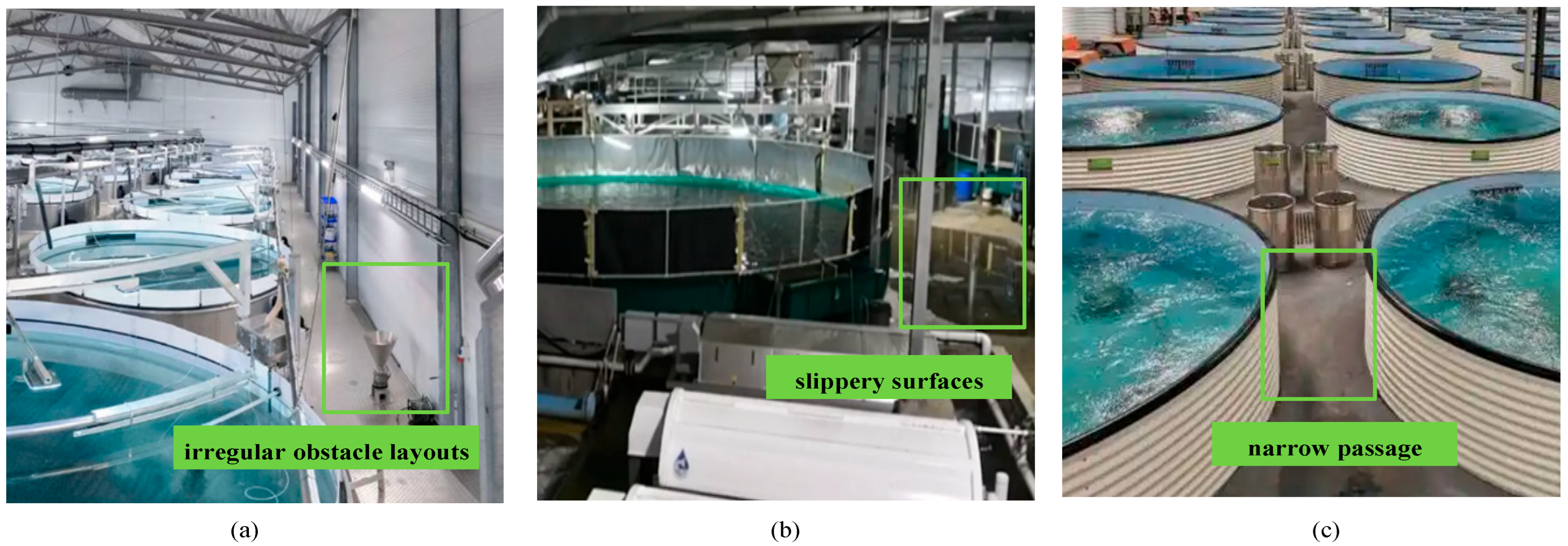
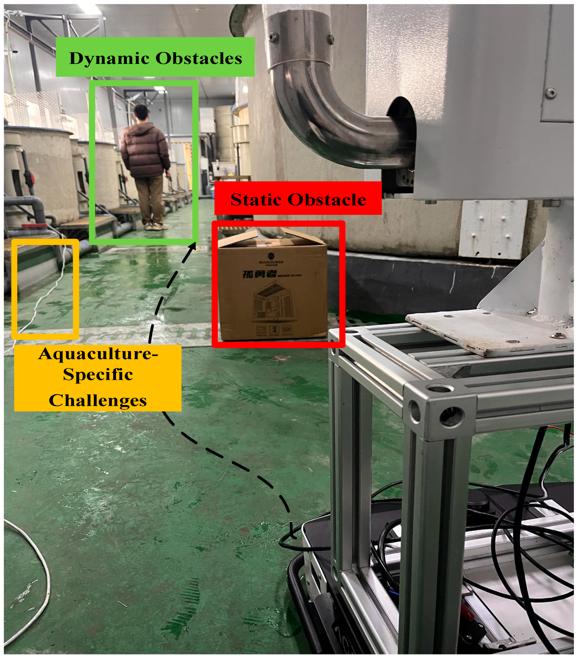
Figure 1.
Issues in the RAS environment: (a) Irregular obstacle configuration. (b) Slippery surface. (c) Constricted passage.
Figure 1.
Issues in the RAS environment: (a) Irregular obstacle configuration. (b) Slippery surface. (c) Constricted passage.
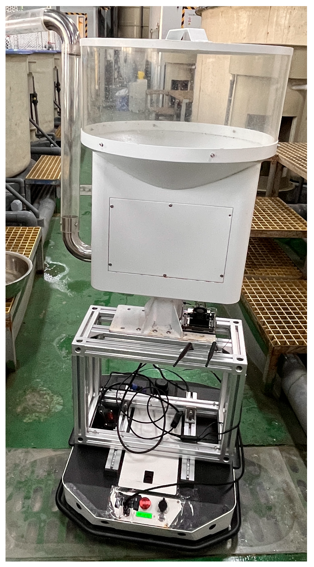
Figure 2.
Experimental testing scenarios for AGV in the RAS environment.
Figure 2.
Experimental testing scenarios for AGV in the RAS environment.
Figure 3.
Integrated framework for path planning using NRBO-ACO and dueling DQN.
Figure 3.
Integrated framework for path planning using NRBO-ACO and dueling DQN.
Figure 4.
Obstacle threat cost analysis for fish tanks.
Figure 4.
Obstacle threat cost analysis for fish tanks.
Figure 5.
Distribution and optimisation of path nodes in narrow passages.
Figure 5.
Distribution and optimisation of path nodes in narrow passages.
Figure 6.
Logical framework of the NRBO-ACO algorithm.
Figure 6.
Logical framework of the NRBO-ACO algorithm.
Figure 7.
Architecture of the dueling deep Q-network.
Figure 7.
Architecture of the dueling deep Q-network.
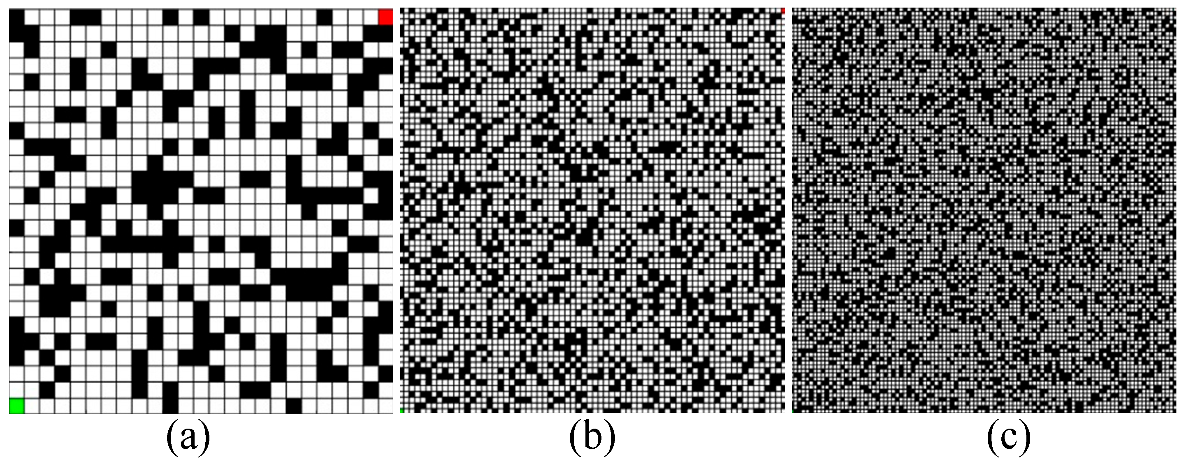
Figure 8.
Random grid maps with varying obstacle densities, ranging from (a) 25 × 25, (b) 70 × 70, (c) 100 × 100.
Figure 8.
Random grid maps with varying obstacle densities, ranging from (a) 25 × 25, (b) 70 × 70, (c) 100 × 100.
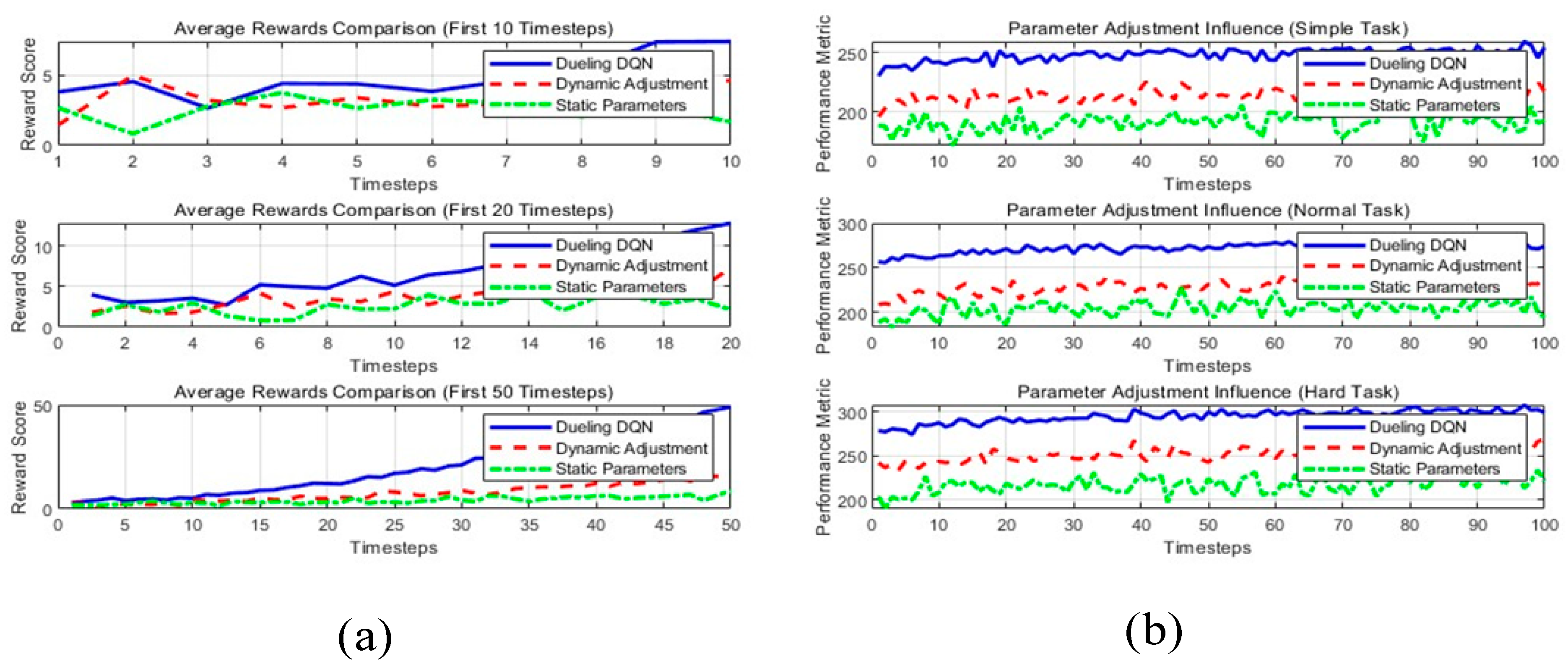
Figure 9.
(a) Comparison of learning speed: dueling DQN vs. alternative approaches. (b) Convergence speed across different task complexities.
Figure 9.
(a) Comparison of learning speed: dueling DQN vs. alternative approaches. (b) Convergence speed across different task complexities.
Figure 10.
(a) Convergence speed across different task complexities. (b) Computational efficiency across varying task scales.
Figure 10.
(a) Convergence speed across different task complexities. (b) Computational efficiency across varying task scales.
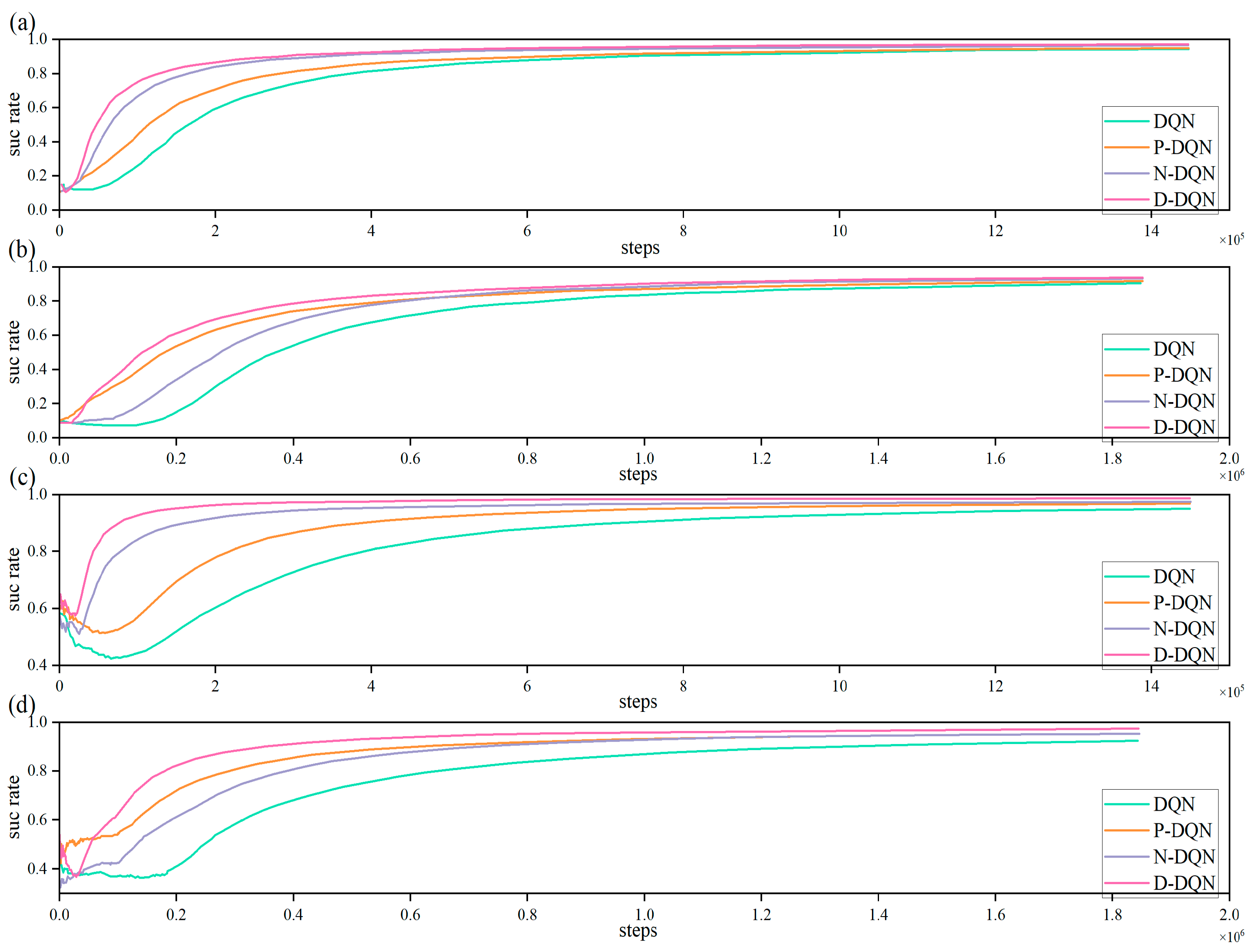
Figure 11.
The success rate and the accuracy of training process. (a) Success rate in 25 × 25 map. (b) Success rate in 70 × 70 map. (c) Accuracy in 25 × 25 map. (d) Accuracy in 70 × 70 map.
Figure 11.
The success rate and the accuracy of training process. (a) Success rate in 25 × 25 map. (b) Success rate in 70 × 70 map. (c) Accuracy in 25 × 25 map. (d) Accuracy in 70 × 70 map.
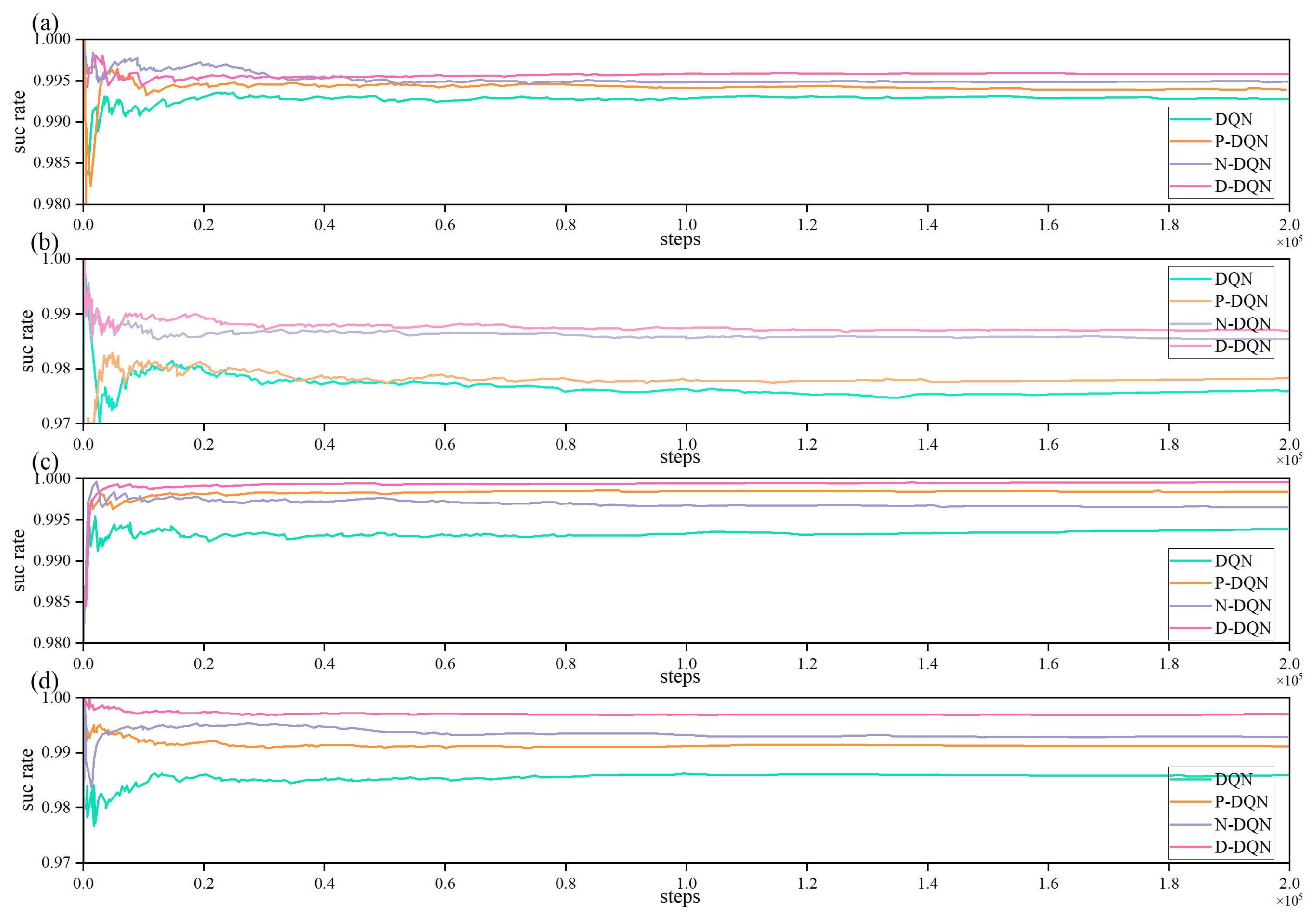
Figure 12.
The success rate and the accuracy of testing process. (a) Success rate in 25 × 25 map. (b) Success rate in 70 × 70 map. (c) Accuracy in 25 × 25 map. (d) Accuracy in 70 × 70 map.
Figure 12.
The success rate and the accuracy of testing process. (a) Success rate in 25 × 25 map. (b) Success rate in 70 × 70 map. (c) Accuracy in 25 × 25 map. (d) Accuracy in 70 × 70 map.
Figure 13.
Path planning outcomes in a random obstacle environment.
Figure 13.
Path planning outcomes in a random obstacle environment.
Figure 14.
Parameter sensitivity analysis for small-scale aquaculture pond (Map 1). (a) ACO, (b) APF-ACO, (c) LF-ACO, (d) NRBO-ACO.
Figure 14.
Parameter sensitivity analysis for small-scale aquaculture pond (Map 1). (a) ACO, (b) APF-ACO, (c) LF-ACO, (d) NRBO-ACO.
Figure 15.
Parameter sensitivity analysis for multi-layer intensive aquaculture workshop (Map 2). (a) ACO, (b) APF-ACO, (c) LF-ACO, (d) NRBO-ACO.
Figure 15.
Parameter sensitivity analysis for multi-layer intensive aquaculture workshop (Map 2). (a) ACO, (b) APF-ACO, (c) LF-ACO, (d) NRBO-ACO.
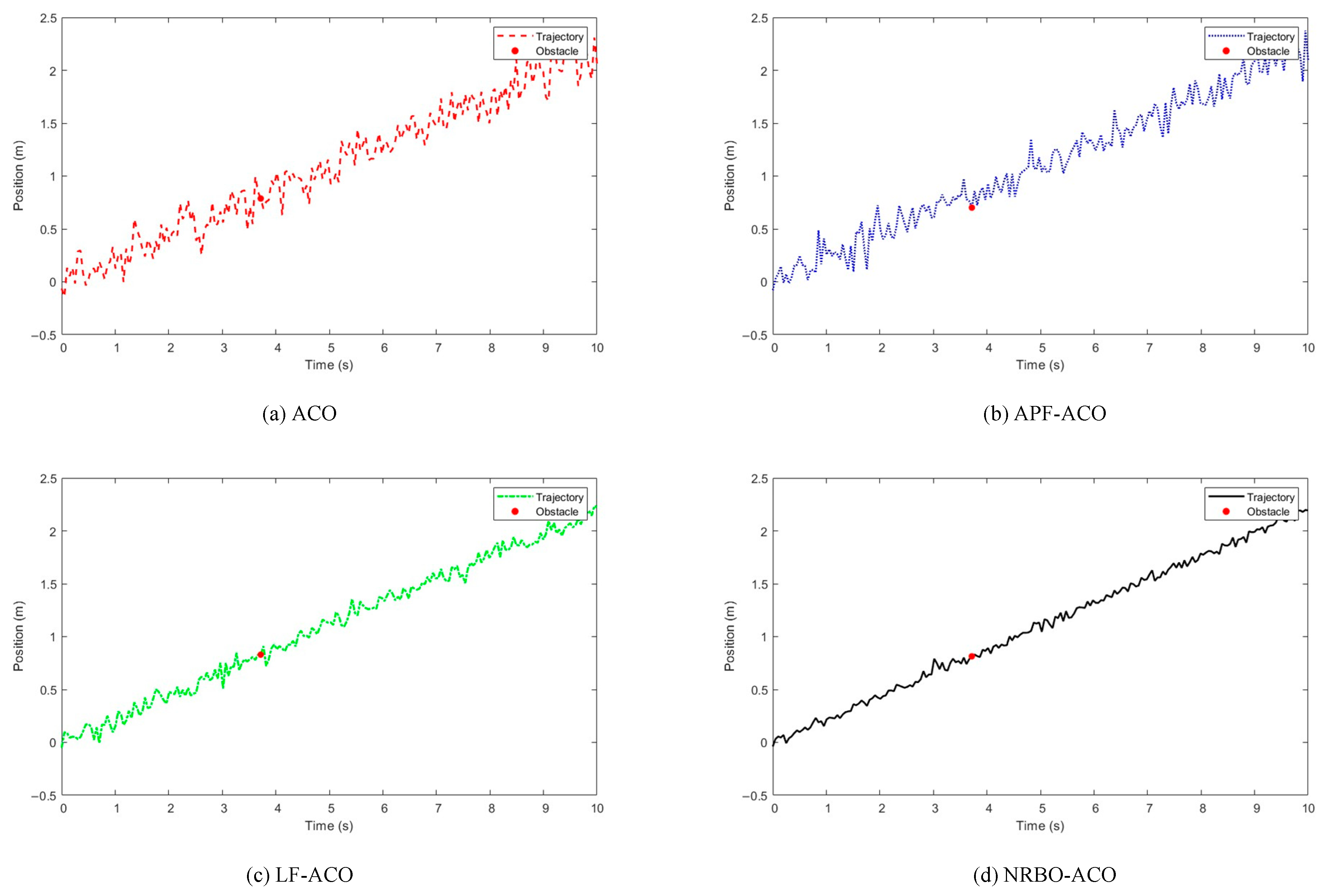
Figure 16.
Parameter sensitivity analysis for single obstacle environment (Map 1). (a) ACO, (b) APF-ACO, (c) LF-ACO, (d) NRBO-ACO.
Figure 16.
Parameter sensitivity analysis for single obstacle environment (Map 1). (a) ACO, (b) APF-ACO, (c) LF-ACO, (d) NRBO-ACO.
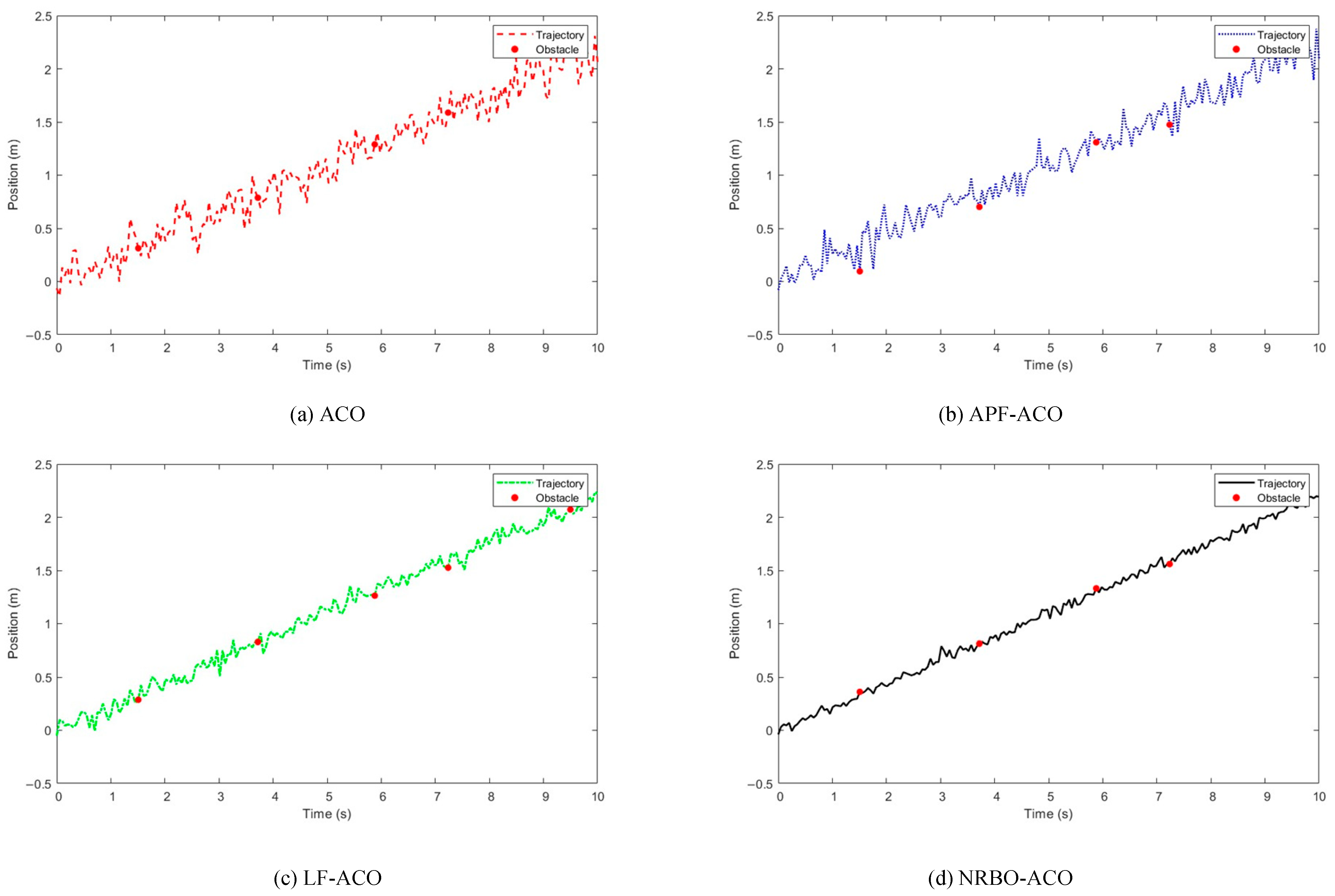
Figure 17.
Parameter sensitivity analysis for five obstacles environment (Map 2). (a) ACO, (b) APF-ACO, (c) LF-ACO, (d) NRBO-ACO.
Figure 17.
Parameter sensitivity analysis for five obstacles environment (Map 2). (a) ACO, (b) APF-ACO, (c) LF-ACO, (d) NRBO-ACO.
Figure 19.
Environmental configuration for the first aquaculture experiment.
Figure 19.
Environmental configuration for the first aquaculture experiment.
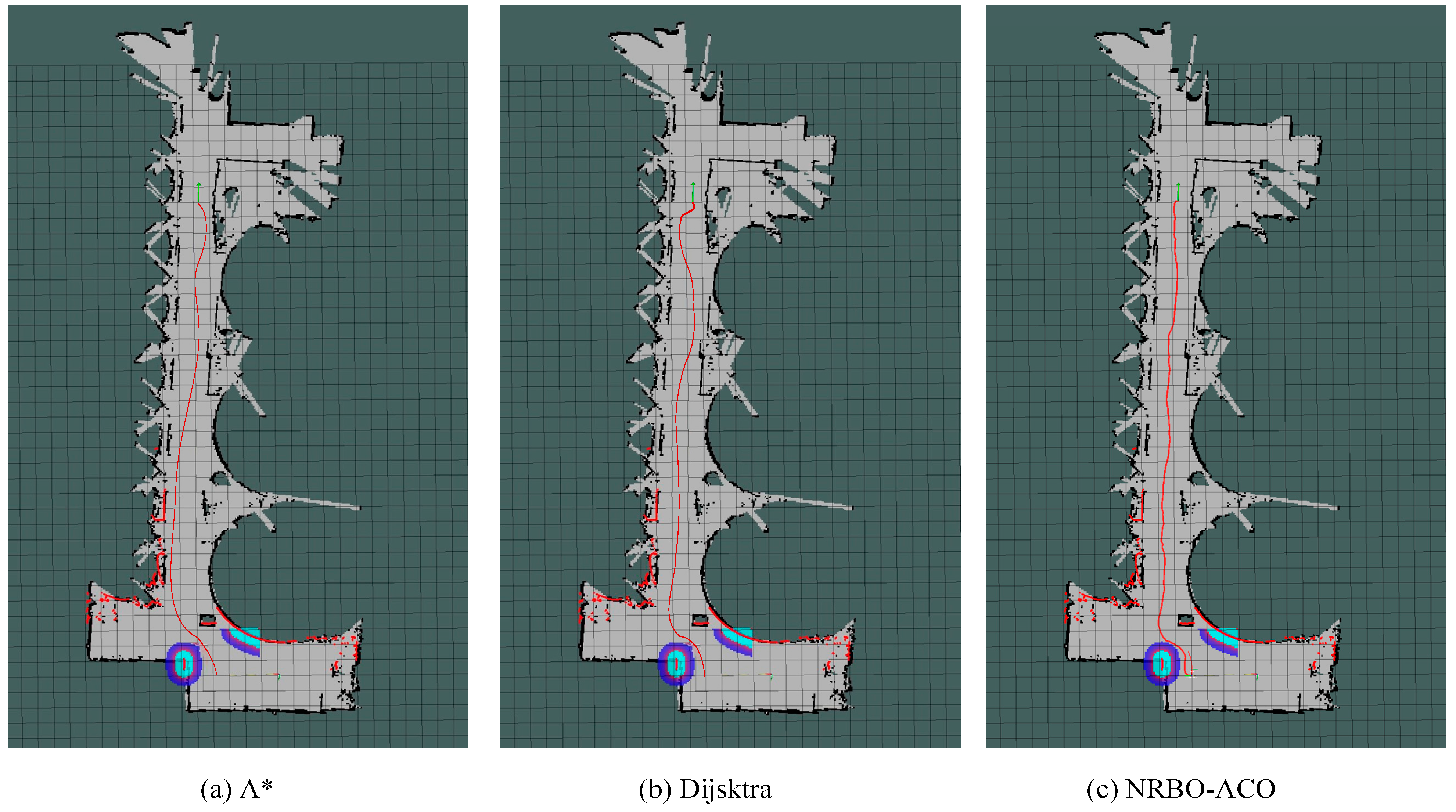
Figure 20.
Path planning results in a simulated aquaculture Environment 1. (a) A*, (b) Dijsktra, (c) NRBO-ACO.
Figure 20.
Path planning results in a simulated aquaculture Environment 1. (a) A*, (b) Dijsktra, (c) NRBO-ACO.
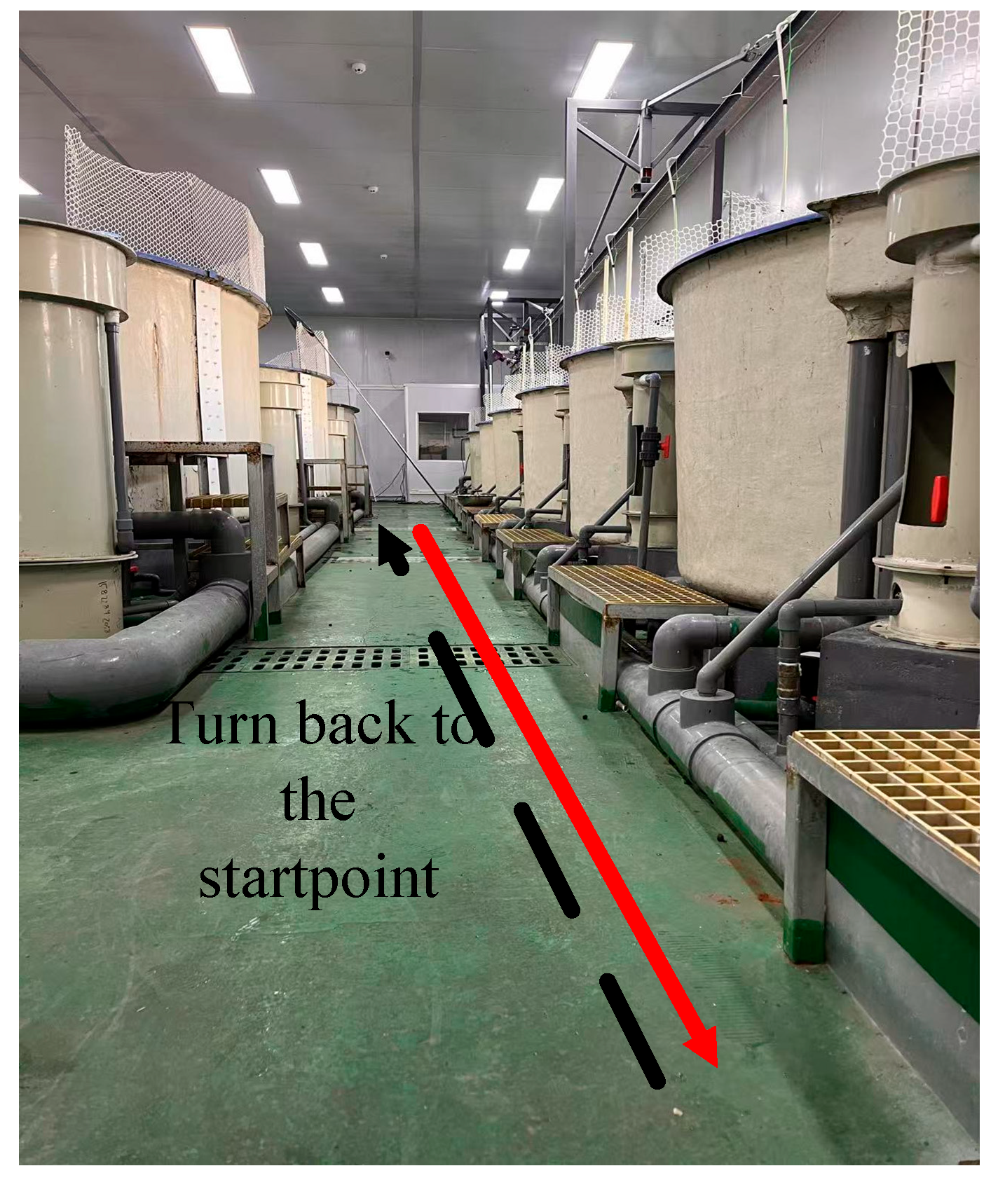
Figure 21.
Environmental setup for the second aquaculture experiment.
Figure 21.
Environmental setup for the second aquaculture experiment.
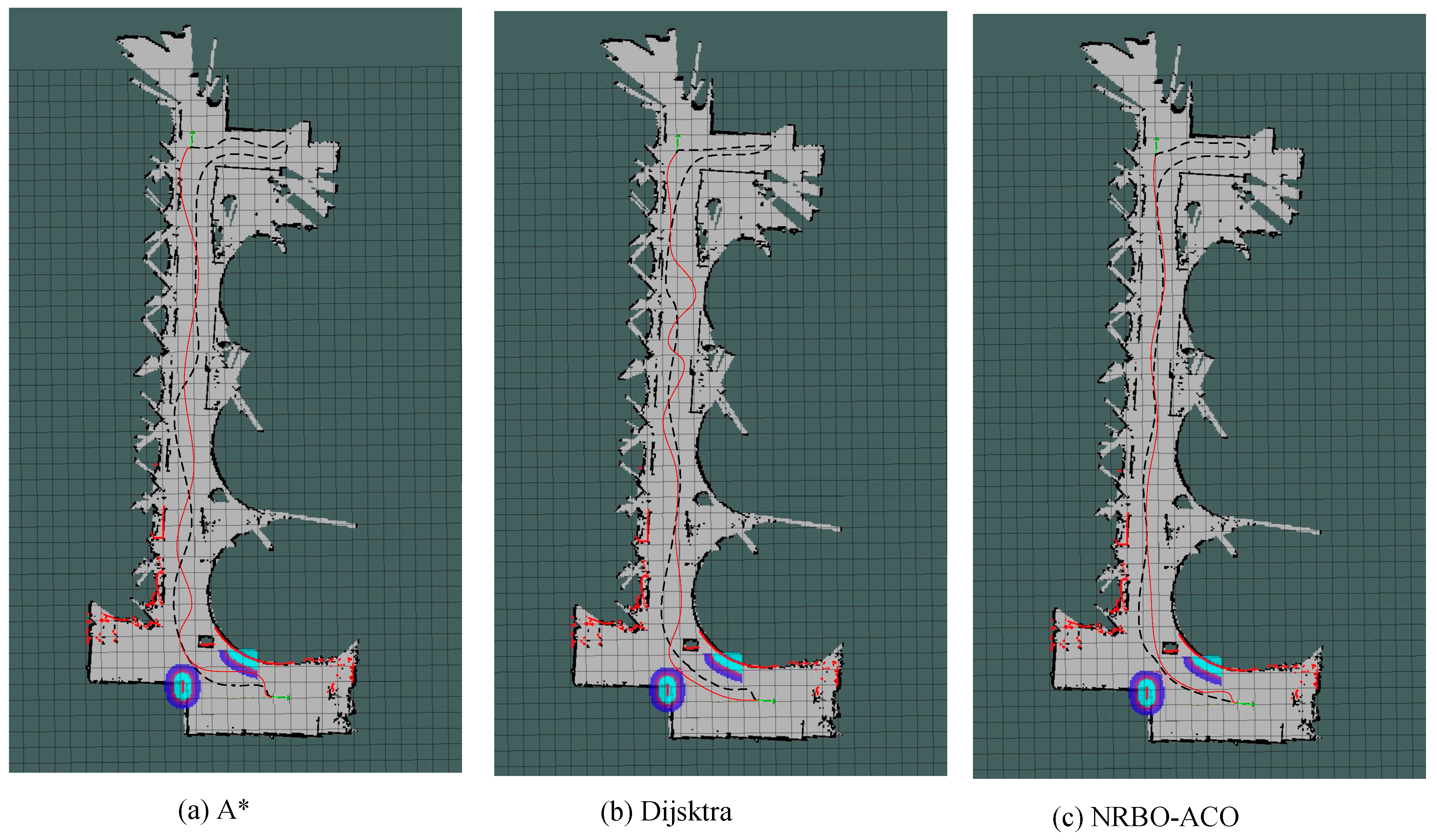
Figure 22.
Path planning results in simulated aquaculture Environment 2. (a) A*, (b) Dijsktra, (c) NRBO-ACO.
Figure 22.
Path planning results in simulated aquaculture Environment 2. (a) A*, (b) Dijsktra, (c) NRBO-ACO.
Figure 23.
Environment and path target setup for the third aquaculture experiment.
Figure 23.
Environment and path target setup for the third aquaculture experiment.
Figure 24.
Path planning results in simulated aquaculture Environment 3. (a) A*, (b) Dijsktra, (c) NRBO-ACO.
Figure 24.
Path planning results in simulated aquaculture Environment 3. (a) A*, (b) Dijsktra, (c) NRBO-ACO.
Table 1.
Learning phases and time steps for dueling DQN evaluation.
Table 1.
Learning phases and time steps for dueling DQN evaluation.
| Learning Phase | Time Steps | Phase Description |
|---|
| Short-term | 10 | Initial learning phase |
| Medium-term | 20 | Intermediate learning phase |
| Long-term | 50 | Long-term learning phase |
Table 2.
Task complexity and grid size for path planning experiments.
Table 2.
Task complexity and grid size for path planning experiments.
| Task Complexity | Grid Size | PII | Phase Description | Path Irregularity |
|---|
| Simple | 25 × 25 | 0.21 | Low-density | Low irregularity |
| Moderate | 70 × 70 | 0.28 | Medium-density | Medium irregularity |
| Complex | 100 × 100 | 0.34 | High-density | High irregularity |
Table 3.
Result of cross-scale evaluation for D-DQN.
Table 3.
Result of cross-scale evaluation for D-DQN.
| Model | Map Size | Success Rate (%) | Accuracy (%) |
|---|
| DQN | 25 × 25 | 97.33 | 99.35 |
| DQN | 70 × 70 | 95.68 | 99.15 |
| P-DQN | 25 × 25 | 98.10 | 99.58 |
| P-DQN | 70 × 70 | 96.47 | 99.20 |
| N-DQN | 25 × 25 | 98.51 | 99.66 |
| N-DQN | 70 × 70 | 98.65 | 99.45 |
| D-DQN | 25 × 25 | 99.65 | 99.97 |
| D-DQN | 70 × 70 | 98.85 | 99.75 |
Table 4.
Initial parameter settings for ant colony algorithm.
Table 4.
Initial parameter settings for ant colony algorithm.
| Parameters | Value | Parameters | Value |
|---|
| Number of ants per metre/m | 500 | Pheromone enhancement coefficient | 10 |
| Initial pheromone value | 1.5 | Heuristic factor | 2 |
| Global pheromone evaporation coefficient | 0.9 | Ant movement step length | 30 |
Table 5.
Simulation data for random obstacle environment.
Table 5.
Simulation data for random obstacle environment.
| Map Size | Algorithm | Avg. Path Length (m) | Std. Path Length (m) | Avg. Runtime (s) | Std. Runtime (s) | Avg. Iterations | Avg. Corners |
|---|
| 25 × 25 | APF-ACO | 34.21 | 2.14 | 0.81 | 0.12 | 16 | 7 |
| LF-ACO | 33.07 | 1.88 | 1.92 | 0.15 | 30 | 7 |
| NRBO-ACO | 32.03 | 1.29 | 0.72 | 0.05 | 13 | 6 |
| 70 × 70 | APF-ACO | 54.94 | 3.65 | 1.95 | 0.21 | 51 | 9 |
| LF-ACO | 58.03 | 2.97 | 4.01 | 0.36 | 72 | 10 |
| NRBO-ACO | 53.01 | 2.11 | 0.97 | 0.05 | 32 | 8 |
| 100 × 100 | APF-ACO | 136.12 | 5.78 | 3.99 | 0.41 | 86 | 10 |
| LF-ACO | 158.89 | 7.24 | 8.11 | 0.51 | 94 | 7 |
| NRBO-ACO | 134.15 | 3.65 | 3.08 | 0.11 | 68 | 7 |
Table 6.
Supplementary smoothness metrics over 100 five-obstacle scenarios.
Table 6.
Supplementary smoothness metrics over 100 five-obstacle scenarios.
| Algorithm | Avg. Jerk (m/s3) | Max Curvature (rad/m) |
|---|
| APF-ACO | 1.97 | 0.58 |
| LF-ACO | 1.72 | 0.44 |
| ACO | 2.35 | 0.65 |
| NRBO-ACO | 0.91 | 0.29 |
Table 7.
Performance comparison of algorithms (30 independent trials).
Table 7.
Performance comparison of algorithms (30 independent trials).
| Algorithm | Map 1 AEI | Map 1 EDI (%) | Map 2 AEI | Map 2 EDI (%) |
|---|
| ACO | 0.82 | 9.7 | 1.24 | 18.3 |
| LF-ACO | 0.78 | 7.2 | 1.13 | 15.6 |
| APF-ACO | 0.73 | 5.9 | 1.05 | 12.4 |
| NRBO-ACO | 0.61 | 3.8 | 0.89 | 6.2 |
Table 8.
Cross-scenario comparison (single and five obstacles).
Table 8.
Cross-scenario comparison (single and five obstacles).
| Algorithm | Scenario | Trajectory Smoothness (σ/m) | Maximum Position Error (m) | Obstacle Distance (m) | Computation Time (s) |
|---|
| ACO | Single Obstacle | 0.10 | 0.15 | 0.15 ± 0.02 | 0.21 |
| | Five Obstacles | 0.12 | 0.31 | 0.18 ± 0.03 | 0.37 |
| LF-ACO | Single Obstacle | 0.07 | 0.12 | 0.18 ± 0.03 | 0.25 |
| | Five Obstacles | 0.09 | 0.18 | 0.20 ± 0.04 | 0.40 |
| APF-ACO | Single Obstacle | 0.09 | 0.10 | 0.20 ± 0.04 | 0.29 |
| | Five Obstacles | 0.11 | 0.25 | 0.22 ± 0.05 | 0.45 |
| NRBO-ACO | Single Obstacle | 0.02 | 0.08 | 0.06 ± 0.01 | 0.15 |
| | Five Obstacles | 0.05 | 0.12 | 0.08 ± 0.02 | 0.25 |
Table 9.
Parameters of the path planning algorithm based on AGV.
Table 9.
Parameters of the path planning algorithm based on AGV.
| Parameter | NRBO-ACO | A* | Dijkstra | TEB |
|---|
| Map resolution (m/cell) | 0.1 | 0.1 | 0.1 | 0.1 |
| Pheromone influence | 1.2 | - | - | - |
| Heuristic factor | 2.5 | - | - | - |
| Pheromone evaporation rate | 0.4 | - | - | - |
| Local planning frequency (Hz) | - | - | - | 10 |
| Slippery zone penalty weight | - | - | - | - |
| Maximum iterations | 500 | 500 | - | - |
| Friction coefficient threshold | 0.3 | - | - | - |
| Step size for Newton–Raphson | 0.02 | - | - | - |
Table 10.
Performance comparison of path planning algorithms in Environment 1.
Table 10.
Performance comparison of path planning algorithms in Environment 1.
| Algorithm | Average Path Length (m) | Average Running Time (s) | Average Corners |
|---|
| A* | 32.4 | 108 | 4 |
| Dijkstra | 30.2 | 100.7 | 4 |
| NRBO-ACO | 28.1 | 70.25 | 2 |
Table 11.
Performance comparison of path planning algorithms in Environment 2.
Table 11.
Performance comparison of path planning algorithms in Environment 2.
| Algorithm | Average Path Length (m) | Average Running Time (s) | Average Corners |
|---|
| A* | 9.5 | 35.7 | 3 |
| Dijkstra | - | - | - |
| NRBO-ACO | 8.6 | 28.6 | 1 |
Table 12.
Performance comparison of path planning algorithms in Environment 3.
Table 12.
Performance comparison of path planning algorithms in Environment 3.
| Algorithm | Average Path Length (m) | Average Running Time (s) | Average Corners |
|---|
| A* | 61.2 | 160.8 | 14 |
| Dijkstra | 59.8 | 154.2 | 11 |
| NRBO-ACO | 56.4 | 121.5 | 5 |


