Optimization of Trailing-Edge Unloading for Lambda-Wing UAV Using B-Spline Trailing-Edge Twist Method

Abstract

As a commonly used configuration for advanced unmanned aerial vehicles (UAVs), the flying-wing configuration suffers from pitching moment trimming issues due to the lack of horizontal tail. The UAV either needs to unload lift at the trailing edge or needs to increase the wingtip twist angle at the cost of losing the lift-to-drag ratio. The commonly used methods for solving pitching moment trimming issues are compared and analyzed in this paper, and it is found that the method of trailing-edge twist has advantages under cruising lift coefficient. Furthermore, a trailing-edge twist deformation parameterized model that can deform multiple critical sections is designed with relevant grids. The multi-objective genetic algorithm is used to optimize the parameterized model and obtain the optimized results. Through comparative analysis, it is found that the optimized trailing-edge twist model has an advantage in distributing the pitching moment. By optimizing the distribution of aerodynamic forces and moments, cruise trim is achieved with only a 1.43% cost to the cruise lift-to-drag ratio compared to the initial model.

1. Introduction

As an advanced design with an updated configuration compared to a traditional configuration, the flying-wing UAV presents more challenges and greater research difficulties. These include the study of aerodynamic optimization and control problems in the cruising state. Nickol et al. [1] conducted research on the aerodynamic performance of a civilian blended wing body (BWB) configuration and found that this configuration offers significant fuel consumption advantages over the traditional configuration, with savings of up to 39%. This underscores the benefits of wing configuration in terms of lift and drag characteristics during cruise. Zhang et al. [2] explored and optimized the relationship between the static stability margin and fuel consumption in the cruising state of the flying-wing UAV design. Their findings revealed that the static stability margin is closely related to fuel consumption. The mechanism behind this is that the static stability margin significantly impacts the configuration design, with a lower stability design leading to improved cruise efficiency. This research provides valuable guidance for the design of flying-wing UAV, suggesting that designers can enhance cruise performance by improving control system capabilities and reducing static stability.

As early as the beginning of 2000, significant research had been conducted on the aerodynamic performance optimization of the blended wing body (BWB) configuration, mainly focusing on wing shape optimization and external drag reduction of BWB [3]. Qin et al. [4] studied the lift distribution and the effect of twist angle on the spanwise lift distribution when optimizing the wing profile of BWB. This study emphasized the ideal lift distribution and the reduction in drag caused by lift-induced vortices rather than torque characteristics. Nevertheless, when studying the configuration of Lambda wings, due to the fact that Lambda wings often exhibit unstable pitching moments at high angles of attack, the process of moment instability is also investigated [5]. Taking Lee et al.’s [6] research as an example, when adding vortex generators to Lambda wings and optimizing the planform, it is necessary to ensure high lift and drag characteristics while also considering the characteristics of high-angle-of-attack pitch moment and increasing the maximum available lift coefficient. However, the moment curve described in this article clearly indicates a zero-lift pitch moment problem, which means that the zero-lift pitch moment remains in a low pitch-down state and requires additional rudder deflection during cruising to achieve normal flight. This problem inevitably leads to increased resistance caused by the control surface, decreasing the cruising lift-to-drag ratio. Even though this was not examined in the article, in practical applications, such a solution would still be unacceptable [7].

A large part of the above research is the result of the combination of Lambda-wing and flying-wing configurations. The pitching moment characteristics at high angles of attack for this configuration are often difficult to directly solve when optimizing this wing configuration combination, but the problem of zero-lift pitch moment is not without a solution. The most common method is to arrange some super heavy equipment behind the UAV. The method of using the engine layout for non-linear trimming mentioned in Mardanpour et al.’s serial articles [8,9,10] can adjust the cruise state moment by adjusting the center of gravity, but it also leads to a decrease in static stability margin. Based on an atypical wing configuration, Mader [11] established an optimization model by changing the wing sweep angle and other configuration parameters, combined with the adjustment of the twist angle, and ultimately improved the pitch moment stability of the model. This research demonstrates the importance of studying the static stability of Lambda-wing UAVs.

However, the configuration design is often constrained by multiple factors at the beginning of the design process. Common approaches to addressing zero-lift pitch moment include replacing the unloaded airfoil, increasing the twist angle and unloading the trailing edge. Tomasz [12] conducted a moment trimming and stability analysis on wings such as canard, flying wing, three-surface tandem wing and box wing and proposed a method of adjusting the moment using weight distribution based on fear of counterweights and structures. Huijts et al. [13] analyzed the drag impact of moment trimming using control surface and proved its side effect on drag force. Karimi et al. [14,15] have focused on the elastic torsion and control systems of wings, aiming to redistribute the aerodynamic moment through elastic torsion and achieve cruise trim state. Syed et al. [16] also analyzed and optimized the aeroelastic process of a flexible airfoil of a flying-wing aircraft with an ultra-long display ratio during deformation. The primary mechanism in this study is the generation of significant post-unloading deformation at the trailing edge of the airfoil. The aerodynamic analysis part includes the process of pitching moment trimming. Xu et al. [17] chose jet flow control for the manipulation and trimming of longitudinal moment. These research studies have demonstrated that the moment trimming process for flying-wing UAVs is a crucial research direction in the design of longitudinal static stability.

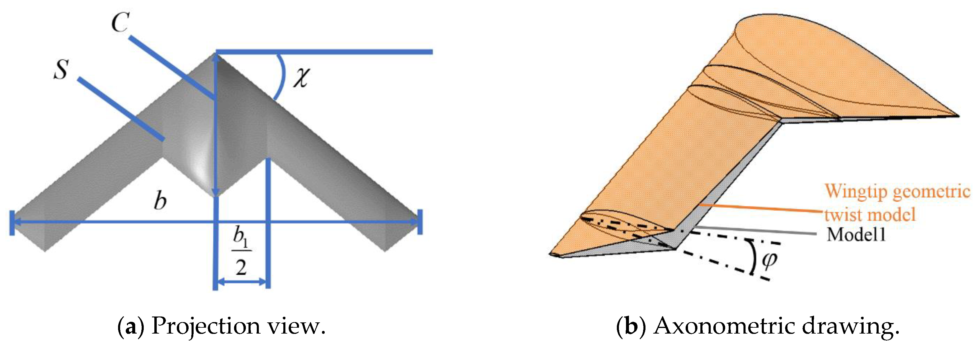
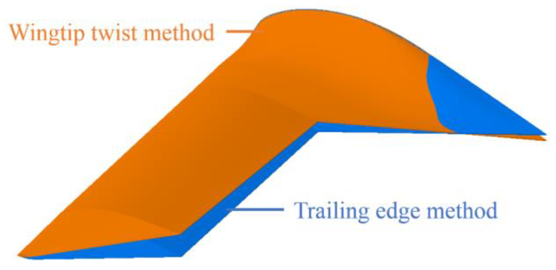
To address the cruise trim moment problem in flying-wing UAVs, various solutions have been explored by scholars worldwide. Common approaches include adjustment of control surface, negative wingtip twist, unloading wing profiles and trailing-edge twist. While adjusting control surfaces is the simplest method, it significantly compromises the lift-to-drag ratio. 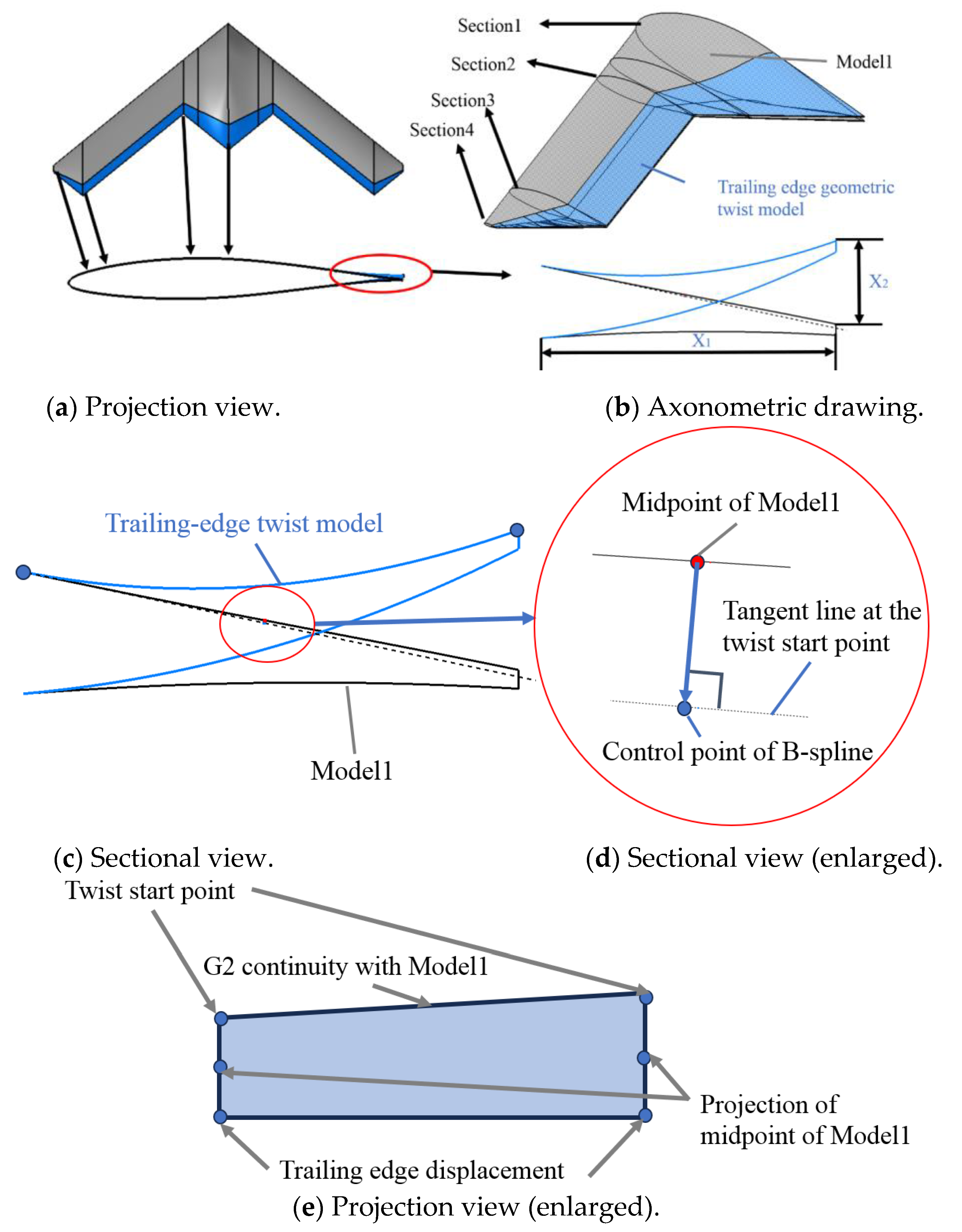For example, the X-47B uses a −10° wingtip twist angle [18] and requires an elevator setting of −23.4° [19] to achieve moment trimming for cruise flight. However, this approach can negatively impact lift distribution and the lift-to-drag ratio. Thus, optimizing wingtip twist angles is essential, either to achieve specific lift coefficients or to maximize the lift-to-drag ratio. Both unloading wing profiles and trailing-edge twist work by reducing lift at the trailing edge to generate a pitch-up moment for trim. However, trailing-edge twist is more versatile, as it directly modifies the wing external shape, offering a broader range of feasible solutions compared to unloading wing profiles.

The advantages and disadvantages of trailing-edge twist and wingtip twist in solving cruise trim problems on a Lambda-wing configuration UAV are analyzed in this paper. A parameterized UAV baseline model with eight parameters for trailing-edge twist is designed and optimized. The analysis results ultimately prove that the trailing-edge twist model improves the degrees of freedom of the model by allowing for the parameter distribution of the twist in multiple sections. And the optimized model redistributes the pitching moment and achieves both drag reduction and trimming.

2. Pitching Moment Trim Problem

2.1. Wingtip and Trailing-Edge Twist Method

In this study, a Lambda wing with parallel leading and trailing edges is adopted as the primary aerodynamic platform for a subsonic UAV. To enhance the structural integration between the wing and fuselage, a thickened root section is designed, allowing the Lambda wing to serve as part of the UAV’s fuselage structure. The key configuration parameters of the Lambda wing include the wing area S, sweep angle χ, wingtip twist angle φ, chord length C, wingspan b and inner wing span b₁, as illustrated in Figure 1.

Given the geometric constraints inherent to Lambda-wing UAVs, this paper replaces traditional wingspan and area parameters with a relative aspect ratio for simplification and generalization. Additionally, the trailing-edge turning location is characterized by the ratio b1/b. The baseline and wingtip twist configurations used for aerodynamic and stealth performance evaluation are detailed in

Table 1. Parameters of the wingtip twist model.

Number	Model1	Model2	Model3
S/m2	11.24	11.24	11.24
χ/°	39	39	39
A	4.480	4.480	4.480
φ/°	1.142	5	8
b1/b/%	30.79%	30.79%	30.79%

. The airfoil of all models is NACA64₁212, and the configuration parameters are derived from a previous study [20].

The trailing-edge twist model is shown in Figure 2. Based on Lambda-wing UAV Model1, the trailing edge of the model is displaced upside. The eight curves of the four cross-sections at the trailing edge follow the second-order uniform B-spline rule. Curves generate multiple ninth-order non-uniform rational B-spline (NURBS) surfaces, which ensure G2 continuity with the original model, meaning that the first and second derivatives of the surfaces are continuous, resulting in smooth transitions without visible breaks. NURBS surfaces are defined by a set of control points, weights, knot vectors and basis functions. The high-order continuity of NURBS surfaces can help improve the smoothness of the trailing-edge twist model. The general equation for a NURBS surface is as follows:

$$W\left(u,v\right)={\displaystyle \frac{{\displaystyle {\sum }_{i=0}^n{\displaystyle {\sum }_{j=0}^m{N}_{i,p}(u)M_{j,q}(v){\omega }_{i,j}{p}_{i,j}}}}{{\displaystyle {\sum }_{i=0}^n{\displaystyle {\sum }_{j=0}^m{N}_{i,p}(u)M_{j,q}(v){\omega }_{i,j}}}}}$$

(1)

where $W\left(u,v\right)$ is the surface; $p_{i,j}$ are the control points; $N_{i,p}(u)$ and $M_{j,q}(v)$ are the B-spline basis functions; ${\omega }_{i,j}$ are the weights.

The twist start points of the four sections of the trailing-edge twist model are defined as X₁, and the upward displacement of the trailing edge is defined as X₂. The twist start points of the four sections of the trailing-edge twist model are defined as X₁, and the trailing edge displacement is defined as X₂. This determines the two edge control points of second-order B-splines, and then, the intermediate control points of the second-order B-splines are determined by projecting the midpoint of the twist section onto the tangent line at the twist start point.

Table 2. Parameters of the trailing-edge twist model.

Number	Model1	Model2	Model3	Model4	Model5	Model6
S/m2	11.24	11.24	11.24	11.24	11.24	11.24
χ/°	39	39	39	39	39	39
A	4.480	4.480	4.480	4.480	4.480	4.480
φ/°	1.142	5	8	1.142	1.142	1.142
b1/b/%	30.79%	30.79%	30.79%	30.79%	30.79%	30.79%
Start point of twist B-spline/C	null	null	null	20%	20%	40%
Upward displacement/C	null	null	null	1.2%	0.6%	0.6%

presents the ratios relative to the chord length for models generated via trailing-edge twist modifications of Model1. All other parameters are kept identical to those of Model1. The displacement direction of the trailing edge of these four sections is perpendicular to the wing plane. The eight control points of these four control sections are used to generate the edge B-spline curves of the NURBS surfaces and serve as the edge control points for generating three sets of NURBS surfaces. The remaining control points on the NURBS surfaces are automatically solved by CATIAV5R21 software, constrained by G2 continuity with the wing.

In this paper, the Reynolds-averaged Navier–Stokes (RANS) equation is used as the control equation, and the shear stress transport (k-ω SST) two-equation turbulence model is applied as the CFD method, which is verified using the DLR-F6 Wing-Body model and experimental data provided by 2nd AIAA CFD Drag Prediction Workshop [21]. Due to the extensive CFD calculations involved in subsequent research, the results are closely related to the effectiveness of the grid. An excessively high number of grids will slow down the computation speed, while an excessively low number of grids will decrease the reliability. Therefore, grid sensitivity analysis is necessary. The analysis is carried out by the DLR-F6 model. Grid sensitivity analysis adopts C, M, F and E, referring to coarse, medium, fine and extra-fine mesh levels, respectively.

Table 3. CEM parameters.

Grid Number	Coarse	Medium	Fine	Extra-Fine
Grid nodes	1.20 M	1.81 M	2.72 M	4.09 M

shows the grid resolution from coarse to extra-fine. The four grids follow the rules outlined below:

• All the grids are topologically consistent and shown in Figure 3;
• The far field is ∼20Cref length away from the test geometry;
• The cell size of [C, M, F, E] increases orderly by 1.5 times.

Figure 4 provides an illustration of the grid convergence achieved for the lift coefficient in the test case DLR-F6. The margin of error is the proportion of difference between two lift coefficient results, and the critical convergence of the margin of error is set to 0.5%. Based on the results in Figure 4, the following research will focus on the 2.72M grid.

CFD method verification was conducted using angles of attack ranging from −5° to 2°. The verified lift–drag curve is shown in Figure 5. The grids for the DLR-F6 Wing-Body model and the Lambda wing model are shown in Figure 6. All grid far fields are positioned at a distance 20 times the wingspan of the aircraft, with pressure far-field boundary conditions applied.

Even though there is some fluctuation between this result and experimental data, the verification results still show the feasibility of the numerical analysis method. The aerodynamic computational states of baseline geometry are summarized in

Table 4. CFD parameters.

Flight State Parameter	Value
Static pressure	26,420 Pa
Mach number	0.65
Density	0.412 kg/m3
Temperature	223.15 K
Cruise lift coefficient	0.34
Center of gravity	1.770 m
Mean aerodynamic chord	1.536 m

.

The curves of the pitching moment coefficient and lift coefficient are shown in Figure 7a. The curves of the lift-to-drag ratio and lift coefficient are shown in Figure 7b. Model2 and Model3 represent the wingtip twist models. Model4, Model5 and Model6 represent the trailing-edge twist models. Model5 and Model6 represent the same upward displacement with different twist start points.

From the numerical results, it can be seen that although the long-dashed line representing wingtip twist is effective in trimming the moment coefficient, it causes a significant decrease in the lift-to-drag ratio. The largest drop, up to 3–4, occurs between the lift coefficients of 0.2 and 0.45, including the cruise lift coefficient (0.34). Comparing Model2 and Model3, which also use wingtip twist but with different angles, it can be observed that the moment coefficient increases with the increase in the wingtip twist angle, while the cruise lift-to-drag ratio decreases with the decrease in the wingtip twist angle. If the twist angle is adjusted to maintain trim in the cruise state, there will be a considerable loss in the cruise lift-to-drag ratio, which is detrimental to cruise efficiency.

The numerical results show that the aerodynamic twist and the upward displacement of the trailing edge shift the moment curve upwards, and both parameters significantly affect the cruise lift coefficient and therefore need to be considered. In terms of the lift-to-drag ratio, the aerodynamic twist method has a smaller impact, with smaller loss compared to Model1. The greatest decrease in the lift-to-drag ratio is concentrated around a lift coefficient of 0.5. At the cruise lift coefficient, the drop in the lift-to-drag ratio is only around 1–2.

Comparing Model4 and Model5, it can be noted that the upward displacement of the trailing-edge twist has a significant influence on the pitch moment, with noticeable changes in the lift-to-drag ratio occurring mainly after a lift coefficient of 0.5. However, the lift-to-drag ratio curves for the same upward displacement show good consistency. The starting position of the trailing-edge twist alters the airfoil curvature and affects the moment characteristics, which are notably different from the wingtip twist method. The comparison between the two methods is shown in Figure 8, where blue represents the trailing-edge twist method, and orange represents the wingtip twist method. The starting position of the trailing-edge twist influences the required upward displacement for the trim. The analysis shows that the starting position of the trailing-edge twist is a key parameter affecting both cruise lift-to-drag characteristics and moment characteristics. To accurately find the cruise trim state, it is necessary to optimize these two parameters.

The baseline configuration, Model1, has a very low initial pitch moment at low angles of attack, with a significant gap to meet the requirement of cruise state moment trim, necessitating substantial control surface deflection for the trim. Wingtip twist can effectively improve this characteristic, but increasing the wingtip twist angle to 5° still fails to meet the requirement. Although it can achieve this requirement at a twist angle of 8°, it also proves that this method requires a larger wingtip twist angle. On the other hand, the method of trailing-edge twist approaches the cruise trim requirement while maintaining the lift-to-drag ratio at the cruise lift coefficient, demonstrating its advantage in addressing the cruise state pitching moment trim issue.

According to Figure 7b, the wingtip twist method sacrifices the lift-to-drag ratio at low angles of attack to enhance it at high angles of attack, solving the moment problem. In contrast, the trailing-edge twist method resolves the issue without sacrificing the lift-to-drag ratio at low angles of attack, with a lower reduction at the same lift coefficient. Therefore, subsequent research will focus on optimizing the model using the trailing-edge twist method.

2.2. Optimization Model

Considering the parallel characteristics required by the Lambda-wing flying-wing configuration, the three segments of the trailing edge must remain parallel to the leading edge in the projection view. Therefore, the trailing edge is moved upward in the direction normal to the plane of the leading edge. To ensure the freedom of deformation and computability of the trailing edge, the degree of twist is controlled by upward displacement distance of the trailing edge at four key sections of the Lambda wing. Additionally, in this chapter, the start point of the twist part of each section is controlled by the length rather than the ratio to the chord length used previously. These four parameters control the area affected by the twist part. All trailing-edge twist deformation parameters are shown in Figure 9. The rules for all surfaces remain consistent with the previous chapter.

The quality of the structured mesh is crucial to the fidelity, speed and effectiveness of the optimization process. Since the parametric model designed in this chapter involves trailing-edge twist, using a fixed outer O-block grid generation method will result in inconsistent distances between the upper and lower grids of the wing sections, ultimately leading to variations in the size of the first layer of the grid. The more pronounced the trailing-edge twist, the greater the difference in grid size. The size of the first layer grid affects the wing surface Y+ value, which significantly influences the aerodynamic performance calculations. For the K-ω SST turbulence model, the Y+ value generally should be within 10, with values closer to 1 recommended. Therefore, this study employs the method shown in Figure 10, where the outer O-block nodes follow the trailing-edge twist movement, thus ensuring the consistency of the boundary layer grid thickness. In the study, a parametrically editable script was used to auto-generate grids. Multiple tests proved the high success rate of this grid generation method.

In the optimization design of trailing-edge twist for trim problems, if only cruise moment optimization is considered, uncertainty in optimization may arise due to multiple shapes satisfying the cruise moment requirements. This can lead to varying losses in the lift-to-drag ratio, potentially degrading aerodynamic performance. The optimization design approach in this chapter aims to maximize the lift-to-drag ratio while maintaining a low trim moment. Therefore, the optimization model can be described as

$$\begin{array}{l}\max \hspace{1em}{F}_{\mathit{obj}1}=L/D\\ \min \hspace{1em}{F}_{\mathit{obj}2}=\left|C_M\right|\\ s.t.\left\{\begin{array}{l}{W}^{″}\left(X{\left(i,j\right)}_{\begin{array}{l}i=1,2,3,4\\ j=1,2\end{array}}\right)=W_0^{″}\\ N_{i,0}^{″}\left(X{\left(i,j\right)}_{\begin{array}{l}i=1,2,3,4\\ j=1,2\end{array}}\right)=N_0^{″}\end{array}\right.\end{array}$$

(2)

where $F_{\mathit{obj}1}$ is the lift-to-drag ratio, and $F_{\mathit{obj}2}$ is the trimming moment coefficient. $W^{″}\left(X,{\left(i,j\right)}_{\begin{array}{l}i=1,2,3,4\\ j=1,2\end{array}}\right)=W_0^{″}$ refers to continuity of the twisted surface at the trailing edge. $N_{i,0}^{″}\left(X{\left(i,j\right)}_{\begin{array}{l}i=1,2,3,4\\ j=1,2\end{array}}\right)=N_0^{″}$ refers to continuity of the cross-section.

Additionally, the lift coefficient of the twisted wing may vary due to changes in the trailing edge at the same angle of attack. Therefore, simply optimizing the lift-to-drag ratio at a specific angle of attack is insufficient. This chapter selects −2° and 2° as the baseline angles of attack. Using a characteristic where the designed lift coefficient lies within the non-separated flow region, a linear fit is performed to find the appropriate angle of attack. Subsequent calculations are based on this new angle of attack. If the new angle of attack calculation meets the required lift coefficient, the results are output. If the new angle of attack deviates significantly from the required lift coefficient, the angle of attack is recalibrated. This recalibration is based on the linear fit of −2°, 2° and the new calculation results. The process is repeated until the fit closely matches the required lift coefficient, and the lift-to-drag ratio and moment are determined and output. If the lift coefficient linearity is still low after too many repetitions, the calculation point will be discarded.

During the optimization design process, the trailing edge is divided into four sections, creating four new sections, resulting in a total of eight variables, including the section twist starting point and the trailing edge upward displacement. The flow chart for the trailing-edge twist optimization model is shown in Figure 11.

The specific variable ranges are shown in

Table 5. Independent variables and their upper and lower bounds.

Variables	X(1,1)	X(2,1)	X(3,1)	X(4,1)	X(1,2)	X(2,2)	X(3,2)	X(4,2)
Lower bound [mm]	50	50	50	10	0	0	0	0
Upper bound [mm]	1000	500	500	50	50	40	30	8

.

In the optimization model, the process for fitting the cruise lift coefficient is as follows: First, using the solved points α = [−2,2], a linear fit of the lift coefficient versus the angle of attack is performed. For example, for Model1, the fitted angle of attack is calculated to be 3.276° from these two points. Then, α = [−2,2,3.276] is used to recalculate the lift. The lift coefficient of the newly obtained point is compared to the design lift coefficient of 0.34, and if the difference is within 0.001, the result is accepted. If the difference exceeds 0.001, a new fitting point is calculated, and the process is repeated. If the fitting process exceeds three iterations without convergence, the calculation point is abandoned. The fitting process is illustrated in Figure 12.

In the optimization model, Latin hypercube sampling was used to generate the initial 64 sample points. This statistical method efficiently generates well-distributed sample points in multi-dimensional space, enhancing sampling efficiency and reducing errors. Unlike simple random sampling, which may result in clustering in certain regions and insufficient converge in others (as seen in Gaussian distribution), Latin hypercube sampling ensures better uniformity with the same limited number of random samples [22]. Efficient sampling models contribute to improving the computational efficiency of optimization models, enabling a quick search for the optimal value across the entire feasible domain and avoiding the pitfalls of local optima. The optimization model employs a non-dominated sorting genetic algorithm (NSGA), a highly robust genetic algorithm offering global search capabilities. The algorithm does not rely on the specific properties of the problem, making it applicable to various types of multi-objective optimization problems. The parameterized model of wing trailing-edge twist used in this paper can seamlessly integrate with NSGA algorithms.

3. Results and Discussion

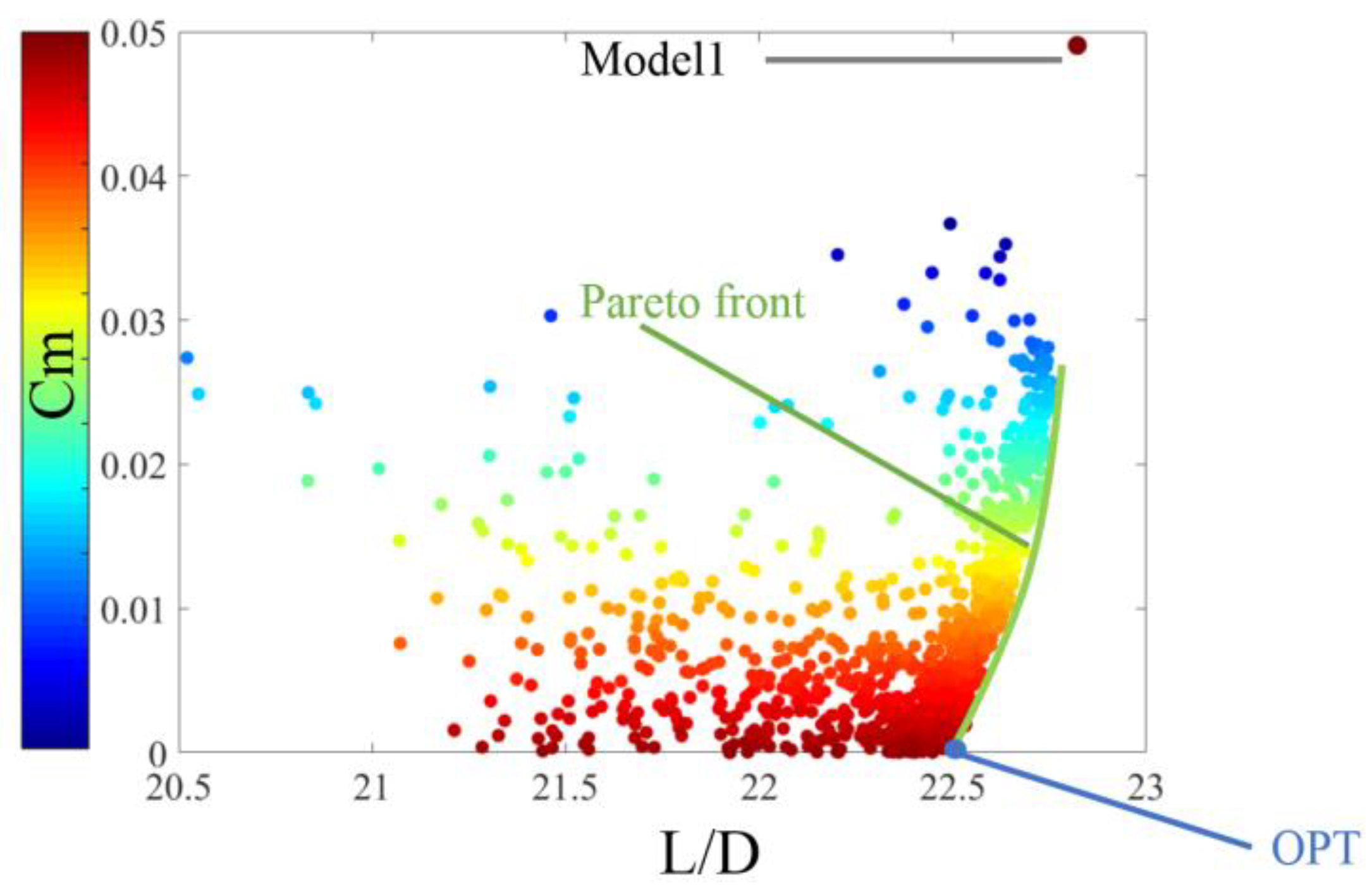
The final results are shown in Figure 13. During the optimization process, a total of 1586 computations were performed, including initial sample points and points generated after iterations. Out of these, 1429 computations were valid. The invalid points included cases of grid generation errors, non-convergent grid computations and failures in the search for the cruising lift coefficient. The optimization results clearly show the Pareto front (points near the green curve). From the Pareto front, the optimal result OPT was selected, marked at the bottom right corner of Figure 13, corresponding to the advantages in moment coefficient and lift-to-drag characteristics. The optimal result OPT is the model where the lift-to-drag ratio is maximized when the trimming moment is less than 2 × 10⁻⁴.

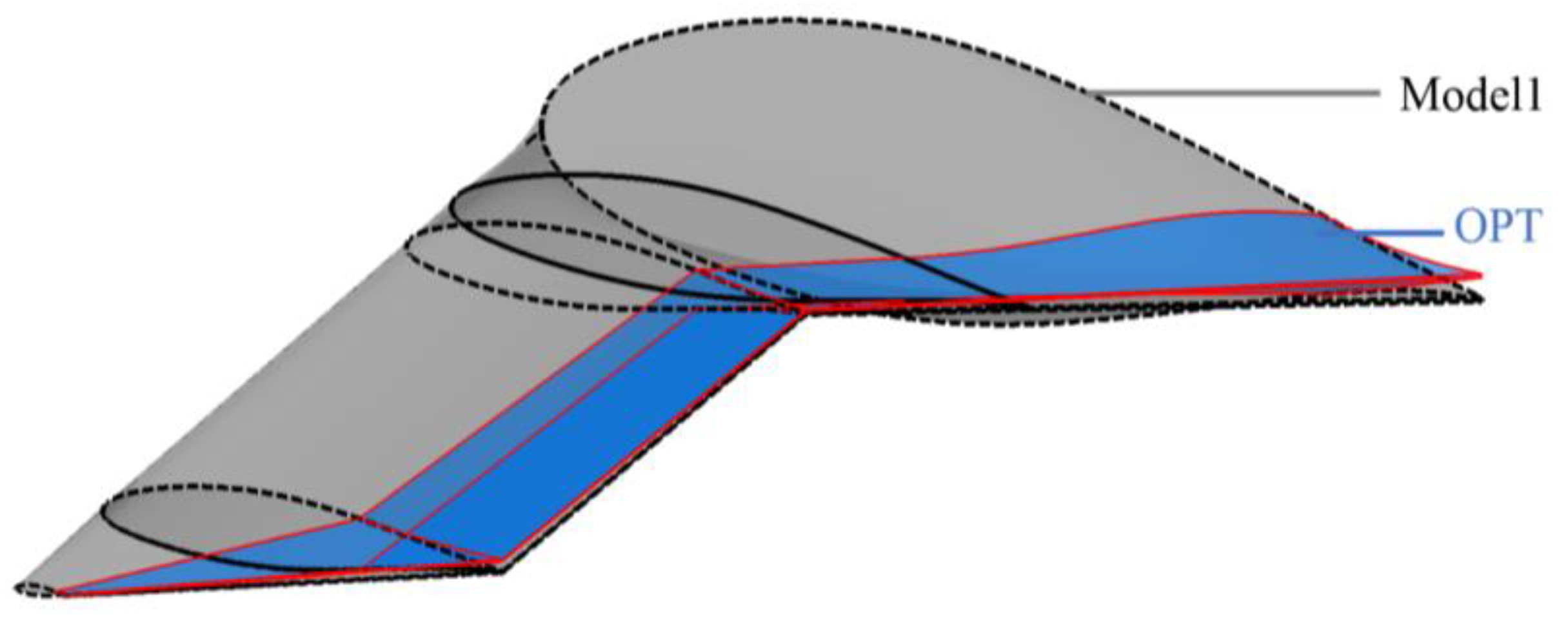
The results indicate that there is a conflict between the pitching moment coefficient and the lift-to-drag ratio within the red Pareto front. A high lift-to-drag ratio implies an increase in trim moment, and an increased trim moment means more control required from the elevator in cruise conditions, which in turn reduces the lift-to-drag ratio. Considering that the main objective of this paper was to achieve trim in cruise state, the model at the bottom right corner was selected. This model is the result of the 1375th computation, which is the 31st individual of the 22nd generation in the genetic algorithm. In the following three generations, no results achieved a higher lift-to-drag ratio with successful trim than this model. This model will be named OPT in the following text. The values of independent variables and values of aerodynamic characteristics are shown in

Table 6. Values of independent variables.

Variables	X(1,1)	X(2,1)	X(3,1)	X(4,1)	X(1,2)	X(2,2)	X(3,2)	X(4,2)
Value [mm]	495.8920	347.1575	448.0385	33.2784	48.3305	6.4116	23.0994	0.1372

and

Table 7. Values of aerodynamic characteristics.

Variables	Lift-to-Drag Ratio	Cruise Pitching Trim Moment Coefficient
Model1	22.822	4.9 × 10−2
OPT	22.492	1.2 × 10−4

. And the comparison of Model1 and OPT is shown in Figure 14.

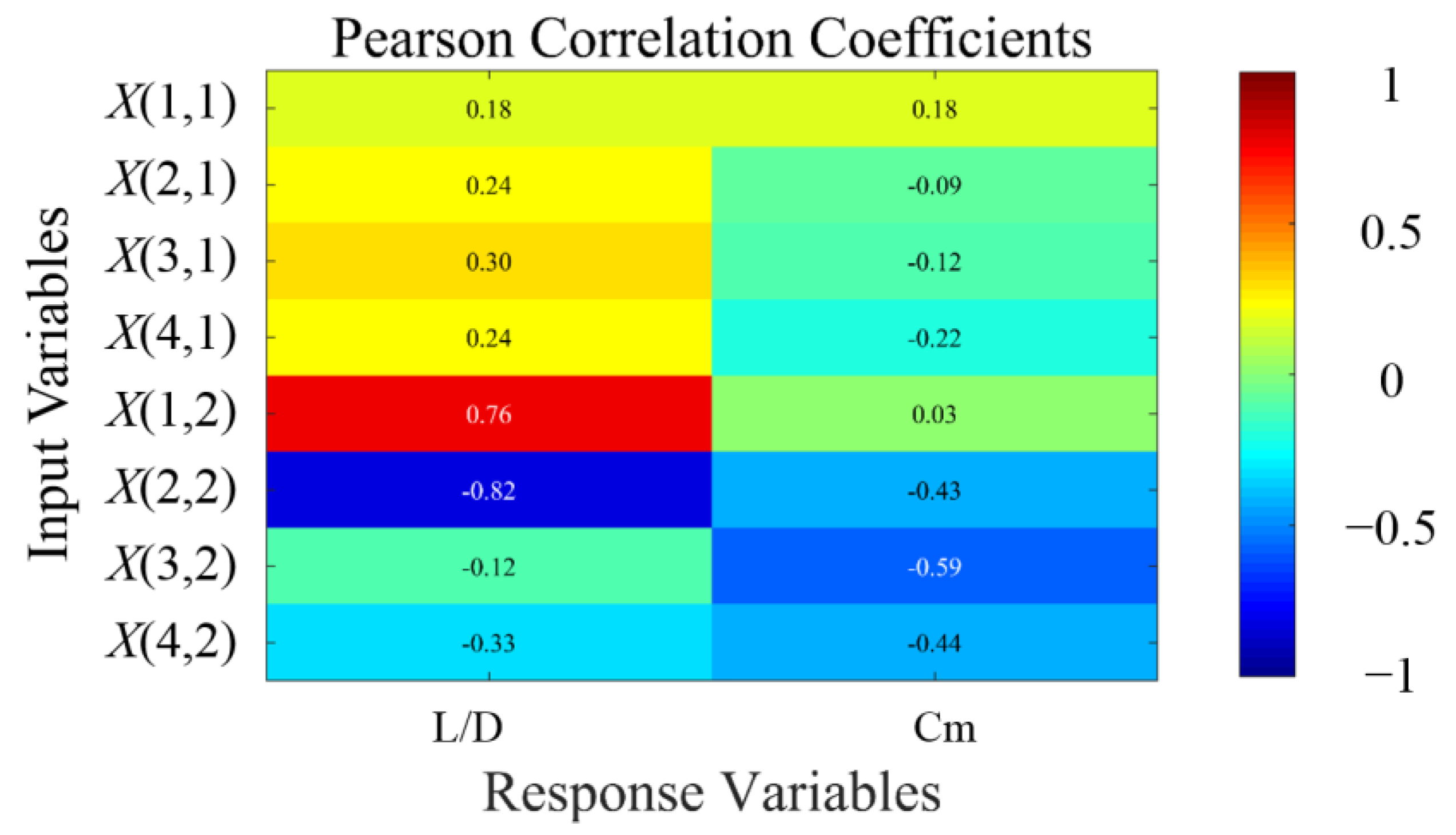
Based on the optimization results, the Pearson heatmap from independent variables to dependent variables is shown in Figure 15. The Pearson correlation coefficient analysis is a statistical method used to measure the strength and direction of the linear relationship between two variables. The Pearson correlation coefficient heatmap provides an intuitive visualization of the correlations among multiple variables. The values of the correlation coefficients fall within the range of [−1, 1], where 1 indicates a perfect positive correlation; −1 indicates a perfect negative correlation; and 0 indicates no linear relationship. The formula for calculating the Pearson correlation coefficient is as follows:

$$r={\displaystyle \frac{{\displaystyle {\sum }_{i=1}^n(X_i-\overline{X})(Y_i-\overline{Y})}}{\sqrt{{\displaystyle {\sum }_{i=1}^n{(X_i-\overline{X})}^2{\displaystyle {\sum }_{i=1}^n{(Y_i-\overline{Y})}^2}}}}}$$

(3)

Here, $X_i$ and $Y_i$ represent the observed values of the two variables; $\overline{X}$ and $\overline{Y}$ are their respective means; and $n$ is the number of observations.

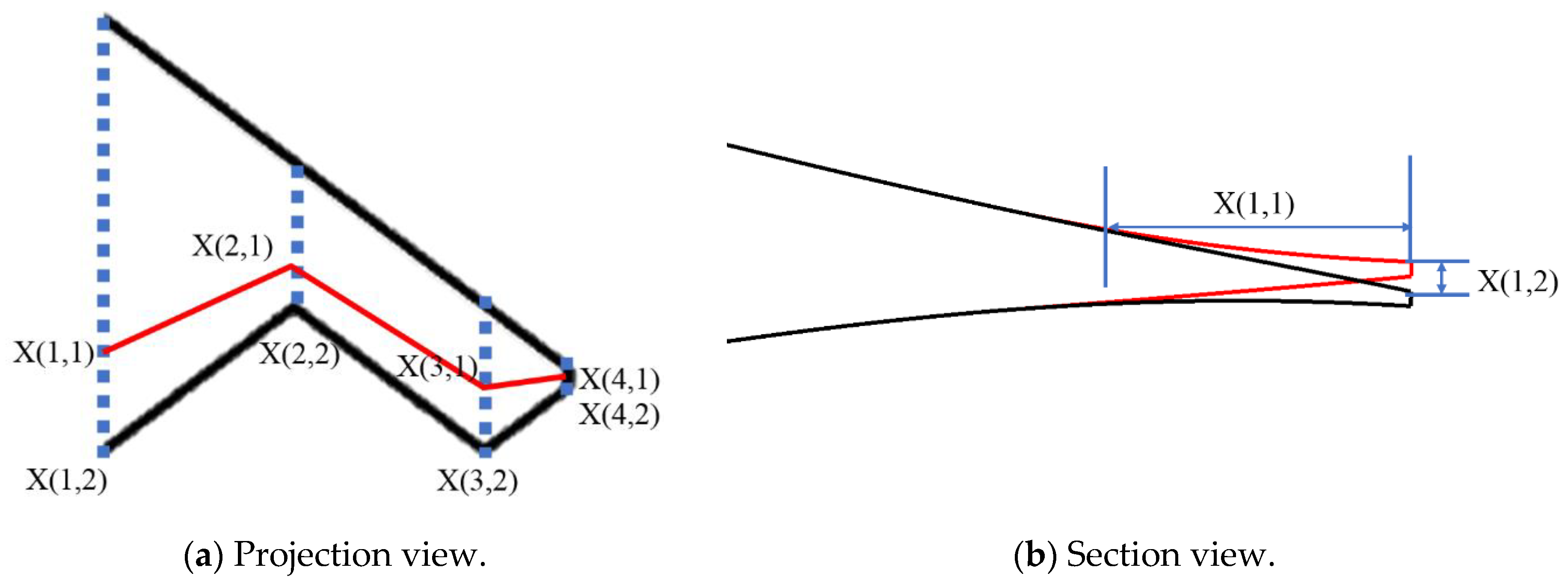
The Pearson correlation coefficient heatmap clearly shows that the two parameters with the greatest influence on the lift-to-drag ratio are X(1,2) and X(2,2), located near the trailing edge close to the wing root. Their correlation coefficients are 0.76 and −0.82, respectively. This indicates that a higher lift-to-drag ratio configuration tends to have more unloading at the trailing edge near the wing root and less unloading in the mid-wing section, with a lower correlation between the wingtip and the lift-to-drag ratio.

Additionally, the heatmap reveals that the parameter with the most significant influence on the cruising pitching moment coefficient is X(3,2) at the third section of the wingtip, with a correlation coefficient of −0.59. Parameters with a moderate influence are X(2,2) and X(4,2), with correlation coefficients of −0.43 and −0.44, respectively. This proves that a lower cruising trim moment means higher unloading at the wingtip. However, it is important to note that in this optimization model, the absolute value of the pitching moment coefficient was used. This means that some models with excessive unloading at the trailing edge were identified as having a high pitching moment coefficient. In other words, due to the absolute value, the moment coefficient appears reduced, suggesting that the actual influence of trailing-edge twist on the trim moment should be higher.

The Pearson correlation coefficient heatmap for the independent variables, as shown in Figure 16, better reflects the coupling correlations between them. Since all correlation coefficients are below 0.5, it can be concluded that the coupling between each pair of parameters is relatively low. The highest correlations are between X(2,2) and X(1,2), and between X(2,2) and X(4,2). This indicates that the linkage between the upward displacement at Section 1, Section 2 and Section 4 is relatively high, while the linkage with Section 3 is lower. The correlations for the start point of the trailing-edge twist are all at low levels, indicating that the start point of the trailing-edge twist has a minimal influence on the section geometry. Instead, it is primarily the upward displacement that affects the unloading force at the trailing edge.

For the aerodynamic analysis of the trim problem, the most critical factor is the pitching moment coefficient. The distribution of pitching moment coefficients at each section of Model1, with the center of gravity as the reference point, is shown in Figure 17. Due to the influence of the area distribution of the Lambda wing, the inner wing section is positioned more forward and inward, thus providing a pitch-up moment. Conversely, the outer wing section extends outward and rearward along the span, gradually providing a pitch-down moment. However, it can be observed that the pitch-up moment in the inner wing section is not linearly distributed, especially near the wing root, where there are fluctuations in the moment provided. Similarly, near the second segment transition at the wingtip, there is also a non-linear characteristic.

The inner wing section provides a pitch-up moment, while the outer wing section provides a pitch-down moment. At the wingtip, the pitch-up moment significantly decreases, which is influenced by the chord length reduction at the outermost part. Nonetheless, this shows that the pitching moment coefficients of each section are not entirely linearly distributed with the wing area and position. Otherwise, the spanwise position from the transition point (1.05 m) to the wingtip (3.4 m) would be expected to show a linear distribution. Comparing the optimized moment coefficients, there is a significant increase in the pitch-up moment at both the wing root and wingtip. The previously fluctuating characteristic of the root pitching moment is mitigated, which aligns with the notable features of X(1,2) and X(3,2) in the optimization results. Between the second and third sections of the outer wing, the moment changes are minimal.

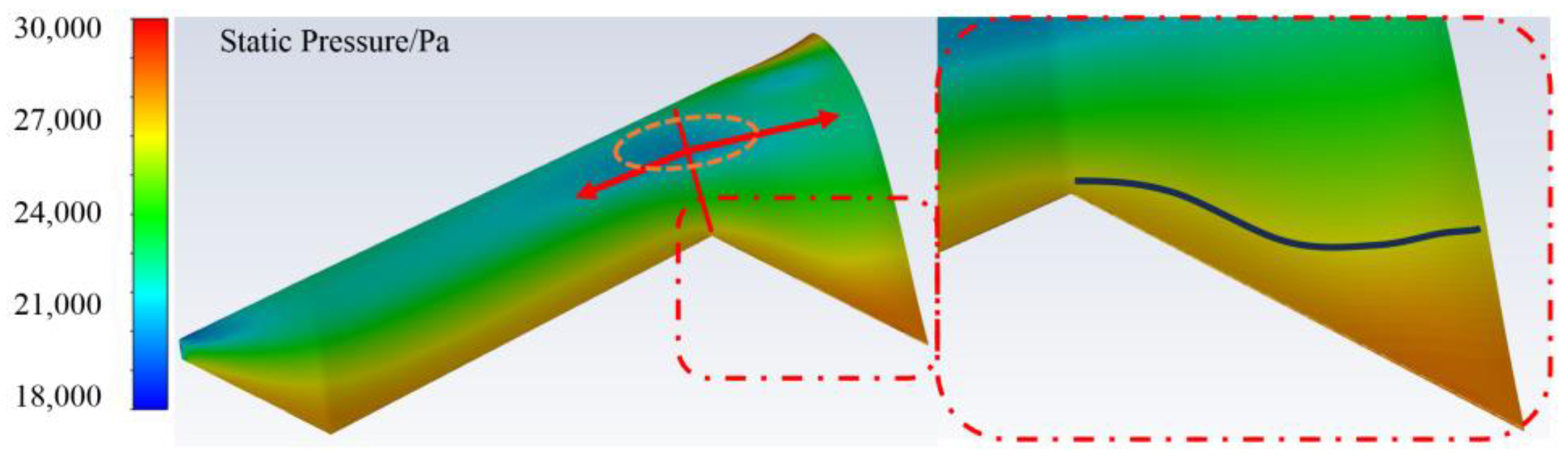
Observing the pressure contour of Model1 in Figure 18, it is clear that the pressure distribution at the trailing edge of the inner wing section aligns with the local fluctuations in the moment curve at the wing root. This characteristic is related to the previously mentioned trend of trailing-edge flow moving toward the wing root. This flow trend becomes more pronounced as the angle of attack increases. Additionally, the pressure contour shows a low-pressure point at the 40% chord line of the transition section. This point extends into an elliptical region both inward and outward, providing suction (the red arrows show the tendency direction). This suction region generates a pitch-up moment but has a weak influence on the wing root, leading to slight fluctuations in the moment coefficient at the root. The elliptical shape of this region also results in the non-linear characteristics of the moment coefficient provided by the outer wing section.

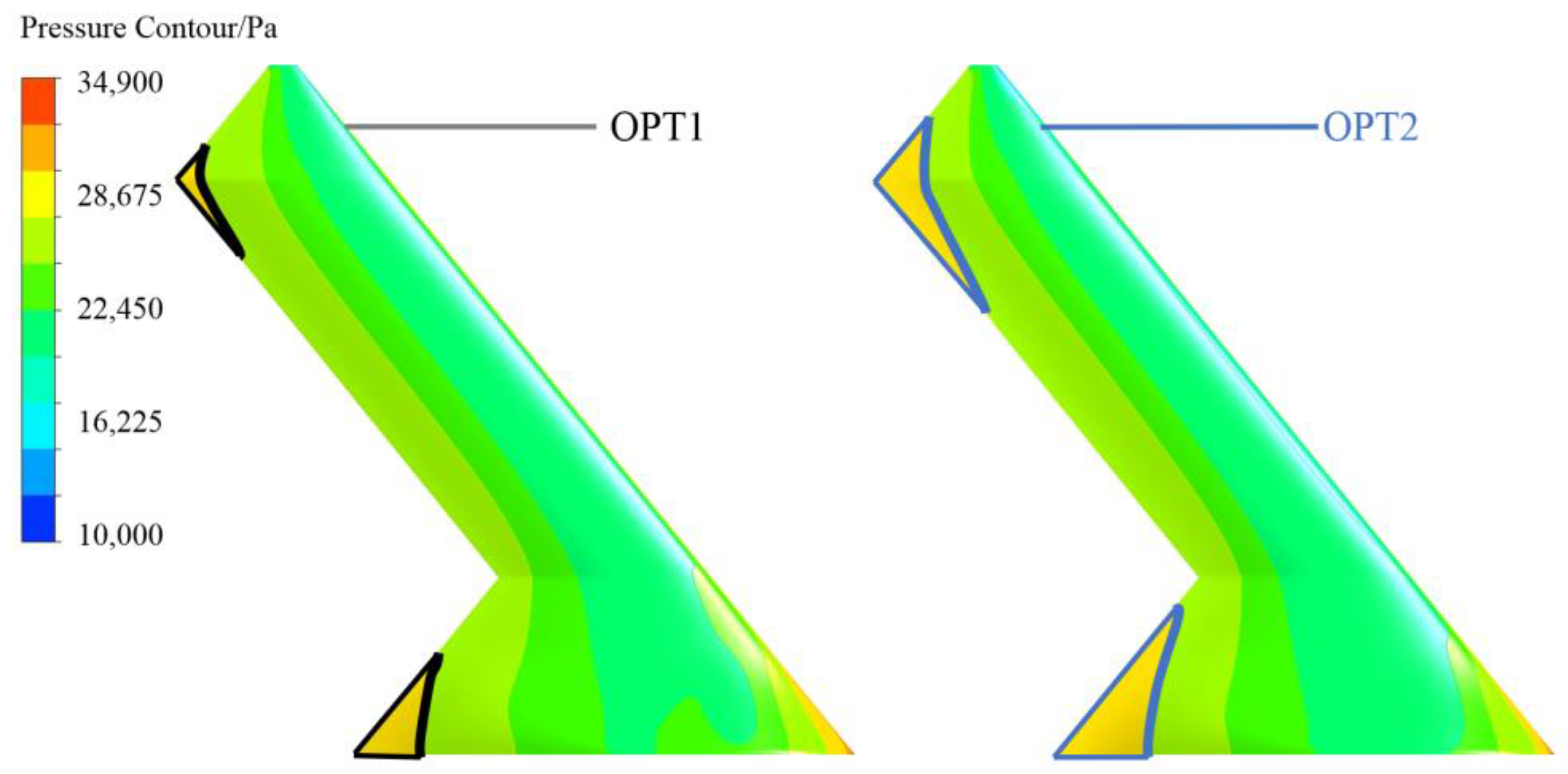
Comparing the optimized results, the surface pressure distribution is shown in Figure 19. The figure shows that the trailing-edge unloading forces are distributed in the regions between the wing root and the second section. This distribution aligns with the characteristics of the moment coefficient decomposition. Specifically, the part of the inner wing near the wing root matches the calculations in Figure 17. In Model1, the moment coefficient at the root exhibits some fluctuation along the spanwise distribution, whereas in the optimized model, the moment coefficient at the root shows a more uniform spanwise distribution. Figure 19 also clearly shows an increase in the trailing-edge unloading area, which in turn increases the root moment coefficient. The characteristics at the wingtip are similar, with a significant increase in the trailing-edge unloading force at the third section, consistent with the features in the moment curve of Figure 17. Additionally, the pressure distribution at the leading edge varies between the two models due to differences in trim angles.

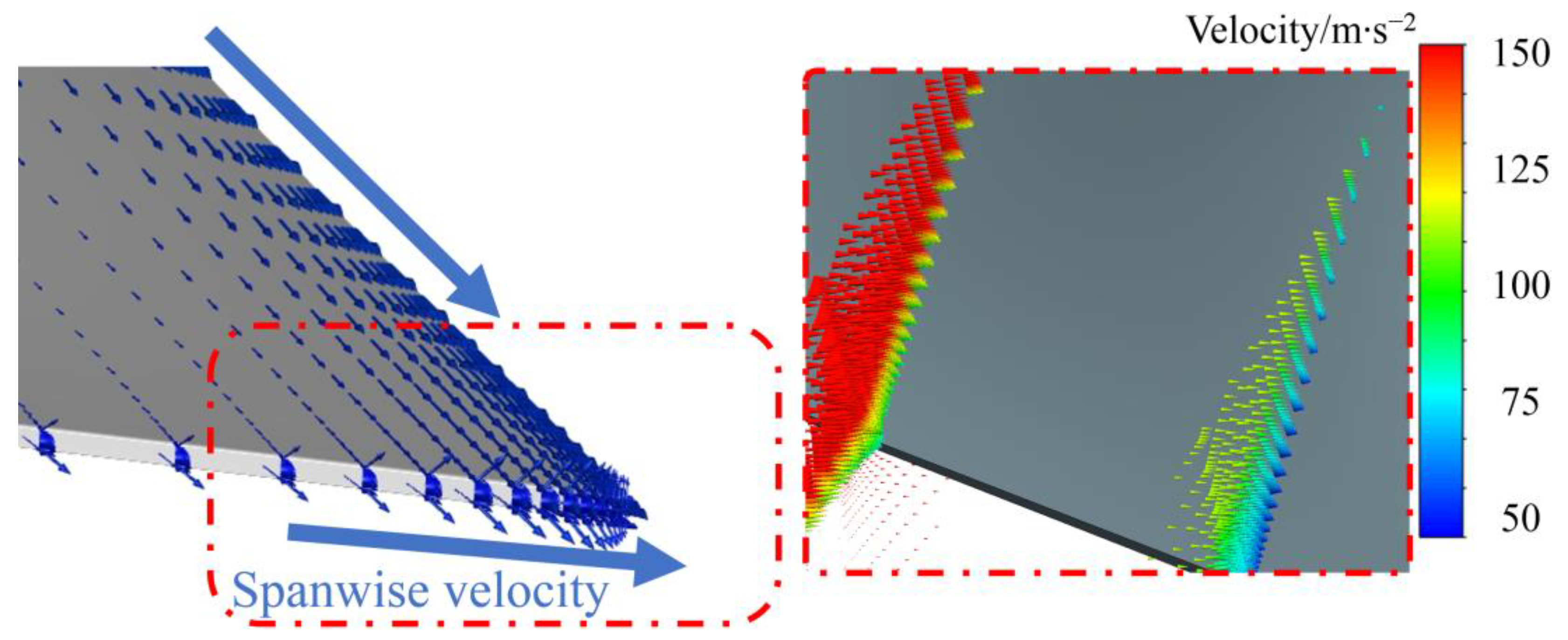
Observing the velocity characteristics in Figure 20, the velocity vectors near the trailing edge of the inner wing comprise a combination of two sets of vectors: one in the direction of the incoming flow and one toward the wing root. The speed in the direction of the incoming flow remains relatively constant because there is almost no separation on the upper wing surface. However, due to the Lambda configuration, there are two sets of spanwise velocities at the trailing edge starting from the second section, moving toward both the root and the third section, with the speed reaching its minimum at the root and the third section. The angle between this spanwise velocity and the incoming flow velocity is acute, meaning that this spanwise velocity accelerates the incoming flow velocity. This results in lower speeds near the root section and the third section compared to other trailing-edge locations during the optimization process, leading to greater trailing-edge unloading forces. This is consistent with the previously mentioned areas that primarily provide trailing-edge unloading forces.

The comparison of lift coefficients in Figure 21 clearly shows that Model1 exhibits a steep drop in lift at the second and third sections. This is an unavoidable characteristic of Lambda-wing design combined with the identical airfoil across the entire wing due to its area rule variations along the spanwise direction. However, the OPT model shows significant changes in lift distribution at the first, second and third sections. The optimized lift distribution becomes more elliptical, which is the main reason for the lower loss in lift-to-drag characteristics after trimming the moment.

Furthermore, observing the drag coefficient, there is an increase in drag around the second section and a decrease around the third section. This corresponds to changes in the lift coefficient and can be considered as variations in the induced drag, having a minimal influence on the overall lift-to-drag ratio. The reduction in lift at the root while maintaining nearly constant drag can be seen as changes in spanwise flow at the root affecting the lift-to-drag ratio. These results are consistent with findings from the Pearson correlation coefficient analysis.

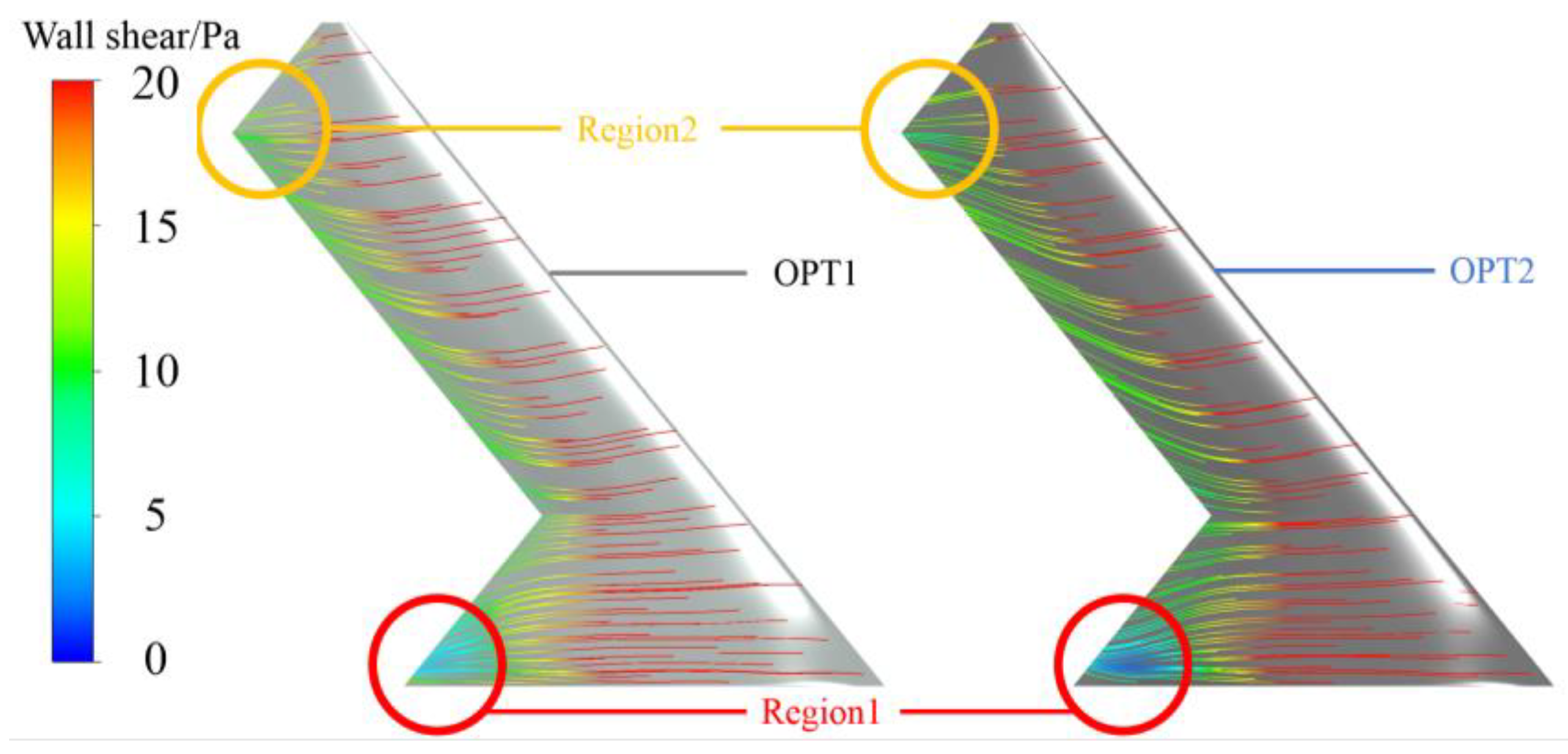
Observing the shear stress streamlines in Figure 22, there is a clear trend of spanwise flow toward the root at the trailing edge. In the initial Model1, this flow starts at the second section and moves toward the root, where it tends to dissipate. In contrast, the OPT model shows a noticeable directional adjustment of this flow near the root (Region1 in Figure 22), reversing the spanwise flow direction before it reaches the root. This change is due to the upward displacement of the trailing edge at the root, making it more difficult for the flow to move toward the root. Similar flow changes also appeared in the third section of the wingtip (Region2 in Figure 22). This positional adjustment corresponds to changes in the lift and drag coefficients near the root. The streamline patterns demonstrate that when trimming the optimized model based on Model1, using a trailing-edge twist model can effectively reduce the additional drag generated by aerodynamic forces. It also keeps the added pitch-up moment within a limited range, thereby ensuring the aerodynamic efficiency of the trimmed model.

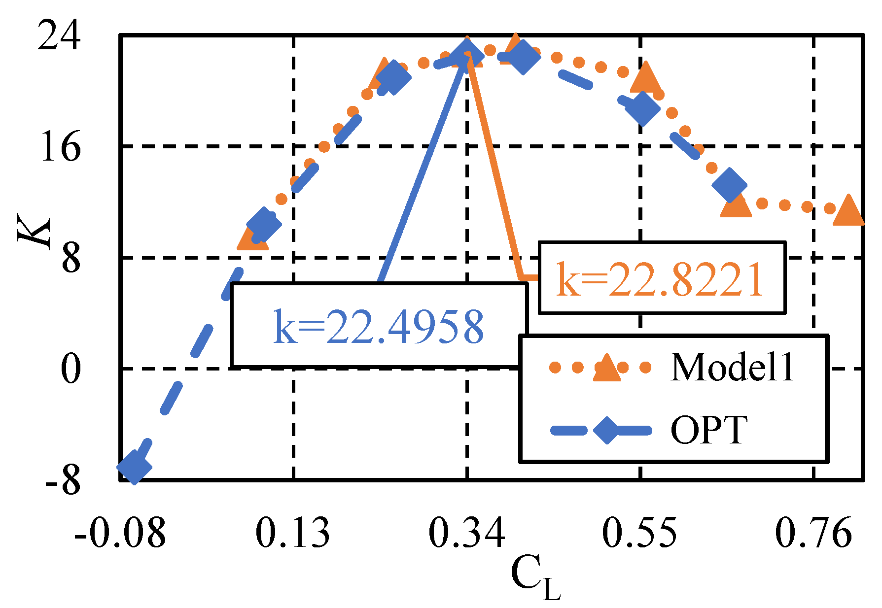
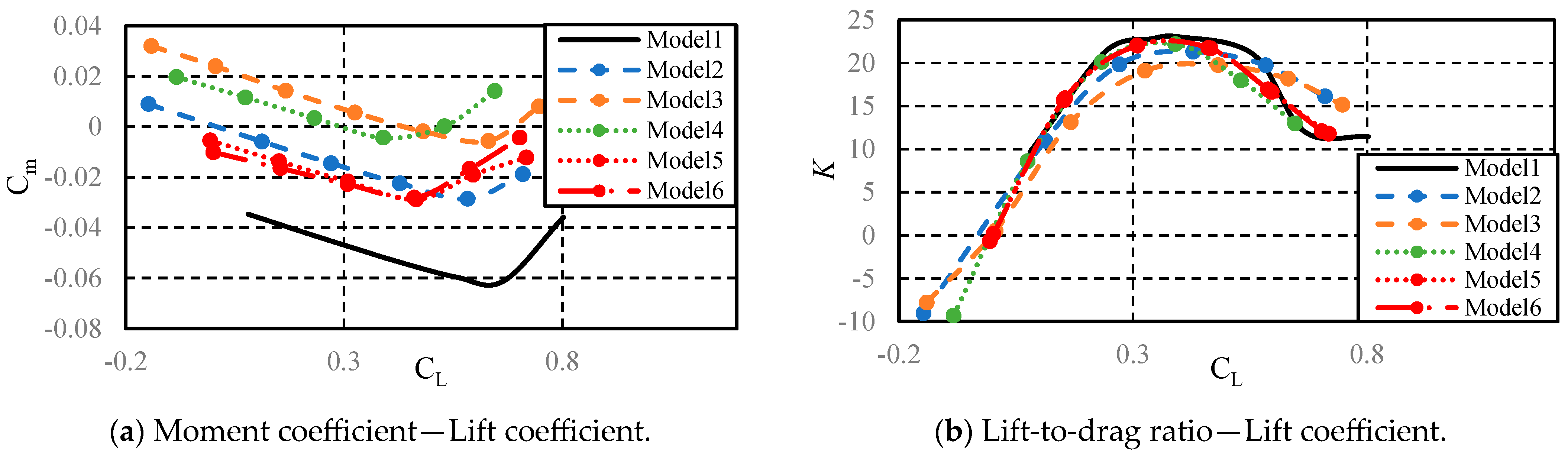
Previous analyses focused on the state of the cruising lift coefficient. Figure 23 compares the lift-to-drag characteristics at different angles of attack. The x-axis is represented by the lift coefficient rather than the angle of attack. This change is due to the significant variations in lift coefficients at the same angle of attack when addressing trim problems. Therefore, using the angle of attack as the x-axis would not provide a meaningful reference. This shows that the changes in the lift-to-drag ratio are minimal at low angles of attack. At high angles of attack and high lift coefficients, there is a slight decrease in the lift-to-drag ratio, but the decrease is within an acceptable range. The change in the lift-to-drag ratio near the cruising lift coefficient is within 3%, which is also within an acceptable range. This indicates that this method is far superior to the wingtip twist method in terms of lift-to-drag characteristics.

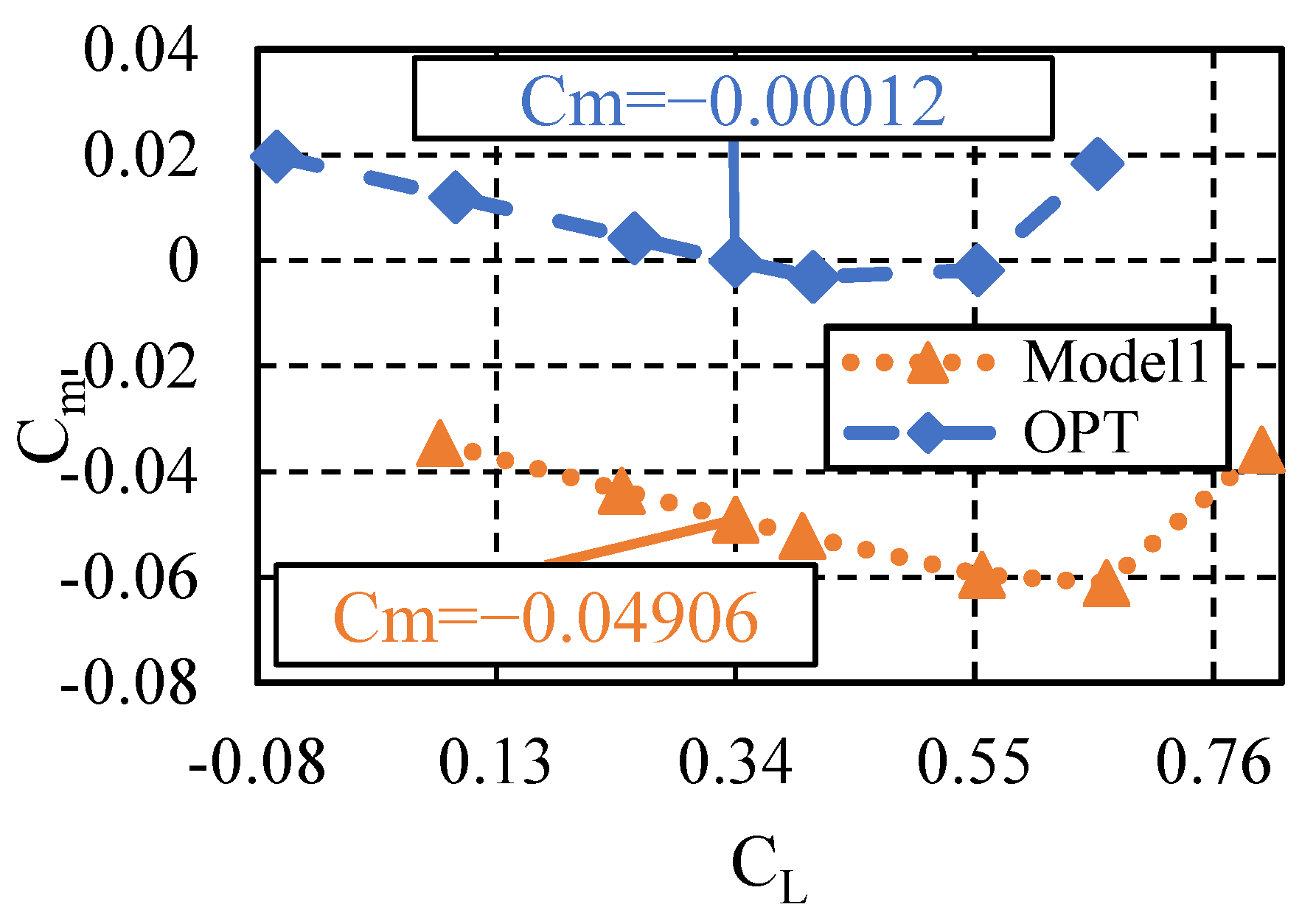
Observing the pitching moment coefficient versus lift coefficient curve in Figure 24, the slope shows minimal variation in the low lift coefficient range, with the static stability margin increasing from 4.4% to 4.9%. The static stability margin is the longitudinal distance between the center of gravity and the aerodynamic center of lift increment, expressed as a fraction of the mean aerodynamic chord, indicating the aircraft’s inherent tendency to return to equilibrium after a disturbance. This phenomenon demonstrates that the aerodynamic center of lift increment in the optimized model shifts forward. The required longitudinal trim moment for cruising conditions significantly decreases from 4.9 × 10⁻² to 1.2 × 10⁻⁴, a value small enough to make the drag loss associated with trim surfaces negligible.

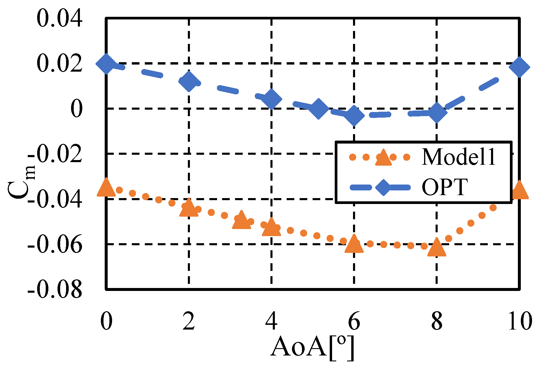
In the optimized model, the reduction in trailing-edge lift leads to a lower lift coefficient, which results in an increased trim angle of attack. Where separation is closely related to leading edge performance, the front edge design of the OPT model remains unchanged. However, with a lower lift coefficient at the same angle of attack, the starting lift coefficient for the static instability region decreases. The region is inevitable in Lambda-wing configurations [23]. This characteristic can be further examined in the moment coefficient versus angle of attack curve shown in Figure 25.

Based on the above analysis, the following conclusions can be drawn: The trailing-edge twist optimization model, after being refined by the optimization algorithm, excels in locally increasing trailing-edge unloading forces. It confines the reduction in lift-to-drag ratio caused by trailing-edge unloading to a small area, thereby having minimal influence on the overall lift-to-drag characteristics during wing trimming.

In terms of multi-angle lift-to-drag performance, the trailing-edge twist optimization model exhibits minimal lift-to-drag ratio loss for the same lift coefficient, showing a significant advantage, especially in the low lift coefficient range. However, due to the model’s inherent principles and the unchanged leading edge, the trailing-edge twist optimization model causes the static instability region at high angles of attack to appear at the same angle of attack as before, leading to an earlier onset of static instability. This characteristic is less favorable for high lift coefficient flight operations. Therefore, this model is more suitable for UAVs designed for long-duration, low lift coefficient cruising.

4. Conclusions

• For the Lambda-wing UAV longitudinal trimming, the wingtip twist method requires a large twist angle, which shifts the peak lift-to-drag ratio to higher lift coefficients and reduces performance at low lift coefficients. In contrast, the trailing-edge twist method effectively preserves the lift-to-drag ratio at low lift coefficients but incurs some loss at high lift coefficients. Under the lift coefficients in this paper, the trailing-edge twist method provides a 14.9% drag advantage.
• Statistically, Pearson heatmap analysis of the optimization results revealed that the variables significantly influencing the dependent variables were concentrated on the trailing-edge upward displacement, with moderate coupling effects observed among trailing-edge twist variables.
• Aerodynamic analysis indicated that the optimized model had a more advantageous force distribution along the span, a lower drag flow characteristic and a more rational trailing-edge unload region. This model achieved a more reasonable transition and enabled longitudinal trimming, with the lift-to-drag ratio reduced by a relatively low 1.43%. This optimization model is highly efficient for longitudinal trimming of Lambda-wing UAVs.

References

1. Nickol, C.; Mccullers, L. Hybrid Wing Body Configuration System Studies. In Proceedings of the 47th AIAA Aerospace Sciences Meeting Including the New Horizons Forum and Aerospace Exposition, Orlando, FL, USA, 5–8 January 2009. [Google Scholar] [CrossRef]
2. Zhang, M.; Chen, Z.; Tan, Z.; Gu, W.; Li, D.; Yuan, C.; Zhang, B. Effects of stability margin and thrust specific fuel consumption constrains on multi-disciplinary optimization for blended-wing-body design. Chin. J. Aeronaut. 2019, 32, 1847–1859. [Google Scholar] [CrossRef]
3. Okonkwo, P.; Smith, H. Review of evolving trends in blended wing body aircraft design. Prog. Aerosp. Sci. 2016, 82, 1–23. [Google Scholar] [CrossRef]
4. Qin, N.; Vavalle, A.; Le Moigne, A.; Laban, M.; Hackett, K.; Weinerfelt, P. Aerodynamic considerations of blended wing body aircraft. Prog. Aerosp. Sci. 2004, 40, 321–343. [Google Scholar] [CrossRef]
5. Shim, H.; Park, S.-O. Passive control of pitch-break of a BWB UCAV model using vortex generator. J. Mech. Sci. Technol. 2015, 29, 1103–1109. [Google Scholar] [CrossRef]
6. Lee, S.; Kim, C. Design Optimization of Lambda-Wing Planform and Vortex Generators for Longitudinal Instability Alleviation. J. Aircr. 2024, 61, 503–514. [Google Scholar] [CrossRef]
7. Taha, H.E.; Hajj, M.R. Optimization of aerodynamic performance and stability of a stealth aircraft. In Proceedings of the 54th AIAA/ASME/ASCE/AHS/ASC Structures, Structural Dynamics, and Materials Conference, Boston, MA, USA, 8–11 April 2013; p. 1674. [Google Scholar]
8. Mardanpour, P.; Hodges, D.; Neuhart, R.; Graybeal, N. Effect of Engine Placement on Aeroelastic Trim and Stability of Flying Wing Aircraft. In Proceedings of the 53rd AIAA/ASME/ASCE/AHS/ASC Structures, Structural Dynamics and Materials Conference, Honolulu, HI, USA, 23–26 April 2012; American Institute of Aeronautics and Astronautics: Reston, VA, USA, 2012. [Google Scholar] [CrossRef]
9. Mardanpour, P.; Richards, P.W.; Nabipour, O.; Hodges, D.H. Effect of multiple engine placement on aeroelastic trim and stability of flying wing aircraft. J. Fluids Struct. 2014, 44, 67–86. [Google Scholar] [CrossRef]
10. Mardanpour, P.; Hodges, D.H.; Neuhart, R.; Graybeal, N. Engine Placement Effect on Nonlinear Trim and Stability of Flying Wing Aircraft. J. Aircr. 2013, 50, 1716–1725. [Google Scholar] [CrossRef]
11. Mader, C.A.; Martins, J.R.R.A. Stability-Constrained Aerodynamic Shape Optimization of Flying Wings. J. Aircr. 2013, 50, 1431–1449. [Google Scholar] [CrossRef]
12. Goetzendorf-Grabowski, T. Flight dynamics of unconventional configurations. Prog. Aerosp. Sci. 2023, 137, 100885. [Google Scholar] [CrossRef]
13. Huijts, C.; Voskuijl, M. The impact of control allocation on trim drag of blended wing body aircraft. Aerosp. Sci. Technol. 2015, 46, 72–81. [Google Scholar] [CrossRef]
14. Karimi Kelayeh, R.; Djavareshkian Mohammad, H. Aerodynamic Assessment of a Control Strategy Based on Twist Morphing Wing in a Flying Wing Aircraft. J. Aerosp. Eng. 2024, 37, 04023087. [Google Scholar] [CrossRef]
15. Karimi Kelayeh, R.; Djavareshkian, M.H. Aerodynamic investigation of twist angle variation based on wing smarting for a flying wing. Chin. J. Aeronaut. 2021, 34, 201–216. [Google Scholar] [CrossRef]
16. Syed, A.A.; Moshtaghzadeh, M.; Hodges, D.H.; Mardanpour, P. Aeroelasticity of Flying-Wing Aircraft Subject to Morphing: A Stability Study. AIAA J. 2022, 60, 5372–5385. [Google Scholar] [CrossRef]
17. Xu, X.; Zhou, Z. Study on longitudinal stability improvement of flying wing aircraft based on synthetic jet flow control. Aerosp. Sci. Technol. 2015, 46, 287–298. [Google Scholar] [CrossRef]
18. Nangia, R.; Palmer, M. A Comparative Study of UCAV Type Wing Planforms—Aero Performance & Stability Considerations. In Proceedings of the 23rd AIAA Applied Aerodynamics Conference, Toronto, ON, Canada, 6–9 June 2005; American Institute of Aeronautics and Astronautics: Reston, VA, USA, 2005. [Google Scholar] [CrossRef]
19. Whittenbury, J. Configuration design development of the navy UCAS-D X-47B. In Proceedings of the AIAA Centennial of Naval Aviation Forum “100 Years of Achievement and Progress”, Virginia Beach, VA, USA, 21–22 September 2011; p. 7041. [Google Scholar]
20. Yuan, C.; Ma, D.; Jia, Y.; Zhang, L. Stealth Unmanned Aerial Vehicle Penetration Efficiency Optimization Based on Radar Detection Probability Model. Aerospace 2024, 11, 561. [Google Scholar] [CrossRef]
21. Eliasson, P.; Peng, S.-H. Drag prediction for the DLR-F6 wing-body configuration using the EDGE solver. J. Aircr. 2008, 45, 837–847. [Google Scholar] [CrossRef]
22. Wang, D.; Lin, J.; Wang, Y.G. Query-Efficient Adversarial Attack Based On Latin Hypercube Sampling. In Proceedings of the 2022 IEEE International Conference on Image Processing (ICIP), Bordeaux, France, 16–19 October 2022; pp. 546–550. [Google Scholar]
23. Yuan, C.; Ma, D.; Jia, Y.; Yang, M.; Zhang, L. Numerical analysis of pitch-break and all moving wingtip aileron of lambda wing configuration. Aerosp. Sci. Technol. 2023, 141, 108508. [Google Scholar] [CrossRef]
Figure 1. Wingtip twist model.
Drones 09 00462 g001
Figure 2. Trailing-edge twist model (the deformation is magnified by 300%).
Drones 09 00462 g002
Figure 3. DLR-F6 block topology and grid resolution (extra-fine and coarse).
Drones 09 00462 g003
Figure 4. Grid resolution convergence results for the normal force coefficient from the grids.
Drones 09 00462 g004
Figure 5. Comparison between the numerical method and the experimental method.
Drones 09 00462 g005
Figure 6. DLR-F6 grid and Lambda-wing grid.
Drones 09 00462 g006
Figure 7. Comparison of moment and lift-to-drag ratio characteristics.
Drones 09 00462 g007
Figure 8. Comparison of the two methods.
Drones 09 00462 g008
Figure 9. Parametric geometry.
Drones 09 00462 g009
Figure 10. Parametric geometry and meshing.
Drones 09 00462 g010
Figure 11. Optimization flow chart.
Drones 09 00462 g011
Figure 12. Fitting the cruise lift coefficient.
Drones 09 00462 g012
Figure 13. Optimized results and Pareto front.
Drones 09 00462 g013
Figure 14. Geometry of Model1 and OPT.
Drones 09 00462 g014
Figure 15. Pearson heatmap from independent variables to dependent variables.
Drones 09 00462 g015
Figure 16. Pearson heatmap between dependent variables.
Drones 09 00462 g016
Figure 17. Pitching moment coefficient distribution at each spanwise section.
Drones 09 00462 g017
Figure 18. Pressure contour of the original model.
Drones 09 00462 g018
Figure 19. Comparison of upper surface pressure distribution.
Drones 09 00462 g019
Figure 20. Wing root spanwise velocity.
Drones 09 00462 g020
Figure 21. Comparison of lift and drag distributions.
Drones 09 00462 g021
Figure 22. Comparison of shear stress streamlines.
Drones 09 00462 g022
Figure 23. Comparison of lift-to-drag ratios between Model1 and the OPT model.
Drones 09 00462 g023
Figure 24. Comparison of moment characteristics between Model1 and the OPT model (pitching moment coefficient versus lift coefficient).
Drones 09 00462 g024
Figure 25. Comparison of moment characteristics between Model1 and the OPT model (pitching moment coefficient versus angle of attack).
Drones 09 00462 g025