Simulation Environment Conceptual Design for Life-Saving UAV Flights in Mountainous Terrain

Abstract

The civil and military use of autonomously or remotely controlled unmanned aerial vehicles (UAVs) has become standard in many sectors. However, their role as supplementary vehicles for helicopter emergency medical services (HEMS) or search and rescue (SAR)—particularly when aiding individuals in hard-to-reach terrains—remains underexplored and in need of further innovation. The feasibility of using UAVs in such operations depends on multiple factors, including legislative, economic, and market conditions. However, the most critical considerations are external factors that impact UAV flight, such as meteorological conditions (wind speed and direction), the designated operational area, the proficiency of the pilot–operator, and the classification and certification of the UAV, particularly if it has been modified for such missions. Additionally, the feasibility of the remote or autonomous control of the UAV in mountainous environments plays a crucial role in determining their effectiveness. Establishing a specialized simulation environment to address these challenges is essential for assessing UAV performance in mountainous regions. This is particularly relevant in the Slovak Republic, a very rugged landscape, where the planned expansion of UAV-assisted rescue operations must be preceded by thorough testing, flight verification, and operational planning within protected landscape areas. Moreover, significant legislative changes will be required, which can only be implemented after the comprehensive testing of UAV operations in these specific mountain environments.

1. Introduction

The constant demand for innovative solutions in the field of aviation, especially in the field of air rescue carried out in mountain environments, has prompted helicopter emergency medical services (HEMS) providers to explore alternative methods to improve the promptness and availability of emergency intervention. In urban areas and relatively easily accessible areas, rescue operations are effectively carried out by ambulances or other special emergency vehicles (quad-wheelers, cars with a doctor, etc.), which ensures the rapid access of medical personnel and equipment to the destination. However, mountainous areas pose significant challenges due to their rugged terrain, limited road infrastructure and unpredictable weather conditions [1,2]. In such areas, HEMS helicopters are the primary rescue vehicle despite their high operating costs, weather-related restrictions, and difficult landing conditions—all of which limit the effectiveness and availability of urgently needed assistance. In extreme cases, rescue teams—such as mountain rescue services—must rely on off-road vehicles or on-foot traversal, significantly delaying emergency interventions [3].

Recent studies suggest that semi-autonomous unmanned aerial vehicles (UAVs) could serve as an efficient, cost-effective supplement to traditional rescue operations. UAVs offer the advantage of rapid response times, reduced mission costs, and accessibility to remote, high-altitude locations, making them a promising alternative for delivering medical supplies, assessing emergency situations, and supporting ground-based rescue teams [4,5]. UAV-assisted operations could notably reduce the number of unnecessary helicopter flights, optimize resource allocation, and enhance survival rates by shortening the critical response times [6,7].

In Slovakia, Air-Transport Europe (ATE)—the exclusive provider of helicopter emergency medical services—has started exploring the integration of UAVs as a supplementary tool for high-altitude rescue missions. UAVs can transport life-saving medications (e.g., defibrillators and first-aid kits), survey hazardous areas, and conduct preliminary situational assessments. These capabilities make UAVs invaluable assets for enhancing efficiency and safety in emergency response operations [7,8,9].

The primary hypothesis underlying this research is that, subject to appropriate and necessary legislative amendments, it is possible to use a suitably modified conventional unmanned aerial vehicle that meets strict criteria in the field of telemetric remote control, enabling a pilot–operator to perform partial (elementary) tasks associated with search and rescue in a difficult-to-reach area. Such a vehicle would provide the possibility of autonomous flight in a determined area even in the event of GNSS signal failures (the authors designed, constructed, and successfully verified and tested the IDVOR navigation system [10,11]); at the same time, the structural modifications made to this vehicle would not pose significant limitations regarding the range, reach, or electromagnetic radiation of the antenna elements of the unmanned aerial vehicle under study (successfully verified and published [12]). The result of the entire process should be a reliable and verified design of a “supplementary rescue unmanned aerial vehicle” (Figure 1), and primarily a simulation environment that can verify its flight in almost-real conditions.

Despite these advantages, the deployment of UAVs in mountainous environments remains a major challenge due to the complex flight conditions, rapid weather fluctuations, and terrain-induced turbulence [13,14]. Designing and developing specialized UAVs for high-altitude applications requires substantial financial investment, and conducting real-world flight experiments in such hazardous conditions carries significant risk. Therefore, rigorous theoretical research must be conducted in parallel with simulation-based testing before moving towards practical implementation [14,15].

Conventional MATLAB-Simulink 2024b UAV models provide a foundational mathematical framework for studying flight dynamics, but they often lack integration with real-time environmental variables. Key limitations include the absence of stochastic wind turbulence modelling, real-time atmospheric variations, and high-altitude pressure differentials. However, recent advances in geospatial modelling, UAV LiDAR data integration, and AI-driven weather prediction systems have led to more precise and adaptive UAV simulations, significantly improving mission planning and operational safety [14,15,16].

This article presents a comprehensive conceptual design for a high-altitude UAV simulation workplace to address these challenges, incorporating real-time weather data, advanced terrain modelling, and AI-based UAV control algorithms. The proposed simulation environment integrates multi-platform software solutions, including MATLAB-Simulink 2024b for UAV dynamics modelling, real-time environmental monitoring, and AI-based trajectory prediction tools [17,18,19,20]. By leveraging high-resolution terrain data, stochastic wind models, and atmospheric pressure variations, this research aims to create a high-fidelity virtual testing ground for assessing UAV behaviour under extreme meteorological conditions.

The integration of simulation-driven insights with real-world UAV flight testing represents a significant step forward in the development of UAV-assisted rescue operations in high-altitude environments.

By establishing a robust, data-driven simulation framework, this research provides a cost-effective alternative to physical UAV testing while enhancing the precision and reliability of UAV performance predictions. This approach improves UAV operational efficiency and safety, and sets the foundation for future advancements in high-mountain aerial rescue missions.

This article’s architecture was systematically constructed in direct alignment with the specific objectives, whose successful fulfilment constitutes the essential prerequisite for achieving the overarching aim. The introduction frames the regulatory, meteorological and topographical obstacles to BVLOS drone rescue in the determined area of High Tatras in Slovakia, establishing the need for a dedicated simulator. Section 2 details the proposed simulation workplace toolchain so that others can replicate it: real-time Meteomatics weather streaming (Section 2.1), terrain and elevation implementation services (Section 2.2), a low-latency Prepar3D-to-Simulink bridge with timing safeguards (Section 2.3), and a full-state quadcopter mathematical model of a modified Mavic Pro UAV from Chinese manufacturer DJI (Section 2.4). Section 3 verifies the designed complex simulation environment by flying four simulated missions from Poprad–Tatry Airport to the Little Cold Valley in the High Tatras, Slovakia, showing displacement errors well within the five-meter delivery target, thereby demonstrating operational credibility. The Discussion section compares the results with the current literature on UAV mountain rescue, highlighting how real-time weather coupling and path optimization reduce risk while still undersampling microclimates. The conclusion outlines the practical implications for emergency medical service providers and maps out future work on higher-resolution atmospheric models and expanded UAV fleets.

2. Creation of the Comprehensive Simulation Environment

A conceptual design of a comprehensive simulation workplace was developed by defining the key input requirements considered throughout the simulation process. These input parameters include the selection of the unmanned aerial vehicle (its mathematical-physical model, electro-mechanical model, transfer function or motion equations), the identification of the designated environment, an analysis of the meteorological and specific conditions within the given area, the design of alternative solutions for search, navigation, or warning systems during UAV flight (including their electro-mechanical and computational models), and the ability to collect and analyze the acquired data for further evaluation. This feature allows for the detailed evaluation of UAV performance, enabling researchers to refine control algorithms, optimize flight paths, and enhance real-time decision-making capabilities.

This conceptual design was preceded by an initial testing and evaluation simulation workplace, which was exclusively based on the MATLAB-Simulink 2024b software environment. However, after conducting the first test flights—both operator-controlled and fully autonomous—it became evident that this approach was insufficient. The primary limitation was the unrealistic scenery, as implementing a fully detailed environmental texture was not feasible.

The simulation workplace concept (Figure 2) shifted after a deeper market analysis of available software solutions capable of conducting simulated flights in external simulation programs, such as SimDirector P3D, RealFlight, and Microsoft Flight Simulator, while maintaining complete integration with MATLAB-Simulink 2024b. Through real-time communication between multiple simulation platforms via the SimConnect API interface, it was possible to leverage the advantages and mitigate the limitations of each specialized simulation software and environment. The elevation points and terrain relief of the designated region, The Little Cold Valley, were successfully generated using the Elevation API software solution and Weather API by Meteomatic, and a test model of the UAV was also successfully implemented.

2.1. Weather API by Meteomatics

As the influence of weather on UAV flights is crucial, we wanted to incorporate this into a complex simulation environment [21,22]. We used the dedicated MATLAB-Simulink 2024b toolboxes (i.e., Aerospace Toolbox), which enable one to perform aerodynamic and environmental effect simulations—such as wind gusts, turbulences and high-altitude atmospheric variations. However, accurate weather data implementation can be performed using Weather API by Meteomatics, which can be described as a high-resolution weather data service that provides real-time and historical weather information for any location on Earth, including mountainous and even rare locations (Figure 3). It is widely used in meteorology, climate analysis, aviation, agriculture, and renewable energy forecasting. It allows users to retrieve temperature, precipitation, wind speed, humidity, air pressure, solar radiation, and other meteorological parameters based on latitude and longitude coordinates [23]. Integrating with MATLAB Simulink enables realistic weather simulations and predictive modelling, allowing researchers and engineers to analyze the weather patterns affecting flight dynamics, autonomous vehicle performance, and energy grid efficiency, in real time and during UAV flight simulation processes. Accurate weather data is crucial for simulating extreme conditions, optimizing energy management in smart grids, enhancing precision agriculture, and improving disaster response strategies. Using the Meteomatics Weather API within MATLAB Simulink, researchers (engineers) can develop real-time weather-adaptive models, optimize machine learning-based climate forecasting, and enhance operational safety and efficiency in weather-sensitive industries—like SAR or HEMS in mountainous environments [24,25,26].

Our objective was to develop a universal simulation environment that accurately reproduces the flight of any drone (represented by a mathematical model) while respecting its kinematics. Our study focuses on a DJI Mavic Pro modified as a technology demonstrator for transporting medicament as an alternative to actual HEMS missions. The mathematic and kinematic models of UAVs were tested and validated in other simulations ([10,11]). The previously performed tests confirmed that the drone modifications leave aerodynamics and kinematics unchanged, and that their influence is negligible compared with meteorological factors.

An analysis of the Little Cold Valley, where the author’s research was conducted, underlined the roles of wind, abrupt temperature shifts, pressure and precipitation in the high-mountain setting, bringing swift, extreme weather changes that undermine flight stability. This air movement is driven by pressure gradient levelling, as low-pressure cores heighten instability. The dominant phenomenon in mountainous areas is the fierce cold Bora wind, which markedly escalates flight risk. It is caused when dense cold air, after surmounting the ridge, plunges leeward and creates mountain waves and rotors. Turbulence in these waves can generate vertical velocities up to 60 m/s. Also, the windward side produces a suction effect, which may cause the UAV to be pulled toward terrain as the lee side imposes sudden downward thrusts.

Mountain-wave simulation, therefore, must count on the ridge height, terrain complexity and wind speed. Alongside Bora, a warm, dry Foehn frequently occurs, rapidly heating and drying the air; the Foehn brings temperature jumps, humidity swings and turbulence that challenge control and sensors. It also brings orographic lift at saturation that yields cloud, fog and persistent precipitation. Another important parameter is the −6.5 °C lapse rate per 1000 m and the dew-point threshold, which causes and accelerates icing. Icing is a dangerous phenomenon as it adds mass, degrades lift and may lead to a loss of control. Moisture also threatens electronics; UAV selection must observe ingress protection as per STN EN 60529 [27]. Vertical shear, mechanical and thermal turbulence, and icing constitute the principal hazards.

Modern simulation platforms let one prescribe wind, gusts, turbulence, humidity and storms. In MATLAB/Simulink, these effects are modelled with environmental blocks in the simulator subsystem. A standard-atmosphere core supplies altitude-dependent profiles of temperature, pressure and density. Parameters can be set manually, generated stochastically or acquired in real time. Merging live data with adaptive control raises the predictive accuracy and safety margins.

In mountain environments, the realistic modelling of wind, temperature, precipitation and pressure underpins every facet of simulated HEMS and SAR drone operations: wind fields dictate real-world moments and turbulence responses, while pressure-driven density and temperature lapse rates set the lift, propulsive efficiency, and climb and range; cold, thin air and headwinds reshape energy budgets, so battery sizing and go/no-go decisions hinge on credible thermal and wind profiles; rain or snow can blind LiDAR, optics and IR sensors, and deep valleys can block GNSS, whereas rapid humidity and pressure swings affect baro-altimeters and IMUs; low temperatures coupled with high moisture cause icing that adds mass and degrades thrust, threatening structural integrity. Crews must rehearse aborts, reroutes and emergency landings in weather-aware simulators because missions rarely wait for ideal conditions; regulators and underwriters demand proof that UAVs can stay controllable within certified wind, temperature and precipitation envelopes, and a data-driven forecast of rotors or microbursts helps prevent an UAV crash into the rescue zone.

The complex simulation workplace could test nominal and extreme scenarios without endangering crew or equipment. Validation is needed to prove that the method reliably predicts drone behaviour under extreme conditions. These findings are pivotal for safe HEMS and SAR missions, where speed and adaptability are vital. Precise UAV kinematics coupled with a detailed meteorological model form the bedrock of autonomous high-mountain operations.

2.2. The Elevation API and Terrain Implementation

Elevation API is a service that provides elevation data for specific locations on Earth. It is commonly used for geospatial analysis, navigation applications, environmental monitoring, and terrain visualization by retrieving elevation values based on latitude and longitude coordinates [28]. When integrated with MATLAB Simulink, it enables realistic navigation simulations in high-mountain environments, allowing researchers and engineers to model terrain, optimize navigation algorithms, and test vehicle dynamics in complex terrains. High-mountain navigation requires accurate terrain data to analyze the altitude variations affecting vehicle performance, simulate GPS (Figure 4) and inertial navigation systems (INS) in rugged environments, test path planning and obstacle avoidance strategies, and model energy consumption and performance for aerial and ground vehicles such as drones and off-road vehicles. Engineers can use realistic, physics-based simulations to enhance autonomous navigation, terrain-adaptive control systems, and the overall vehicle performance in extreme altitudes by leveraging Elevation API data within MATLAB-Simulink 2024b.

The integration of terrain data into a Simulink-based simulation environment is also possible using Digital Terrain Elevation Data (DTED), which enables accurate and efficient real-time elevation lookups. DTED tiles could be preloaded into the system memory to ensure low-latency access during simulation. The dynamic tile management system implemented to load new data only when the simulated aircraft traversed beyond the current tile boundaries is also beneficial. This approach can ensure real-time performance and minimize the computational overhead. In our case, a custom MATLAB Function block was developed to perform geospatial elevation queries using latitude and longitude inputs, incorporating internal unit conversions to maintain consistency with the simulation parameters. The terrain lookup functionality was encapsulated within a modular utility and validated through unit testing to ensure robustness and correctness. For enhanced execution performance and deployment flexibility, the terrain access routines were compiled into MEX functions and integrated into the Simulink environment.

The DTED datasets in our complex simulation workplace were sourced from publicly available repositories, including NASA’s Shuttle Radar Topography Mission (SRTM) and the United States Geological Survey’s EarthExplorer platform. This integration framework offered a scalable and reliable solution for incorporating terrain awareness into real-time simulation workflows. By using the Elevation API or DTED dataset import, the complex simulation workplace could be extended to another areas.

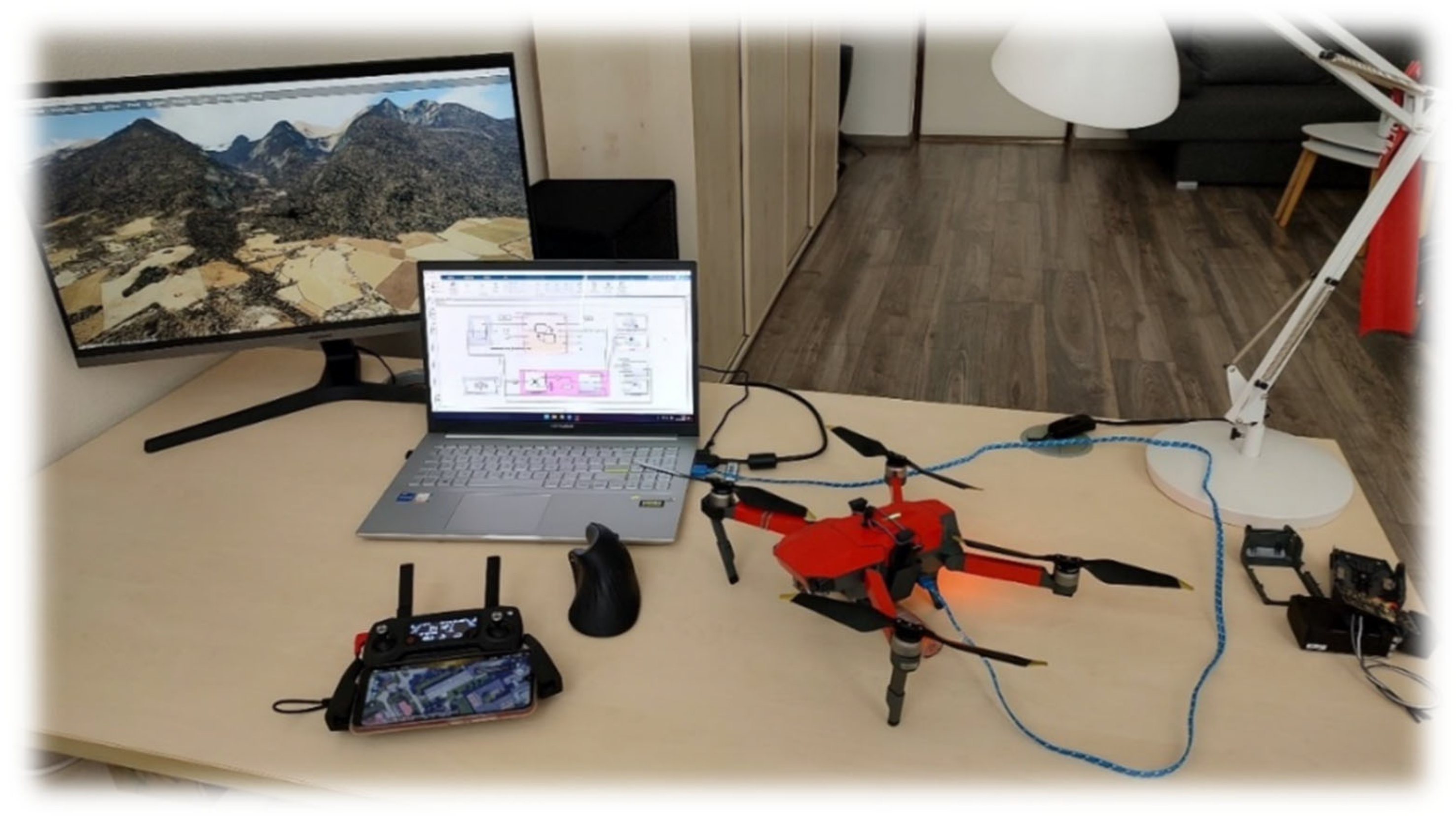
2.3. The Integration of Prepar3D v6.1, MATLAB-Simulink 2024b, Weather API by Meteomatic and Elevation API

In the integration of Prepar3D v6.1, MATLAB-Simulink 2024b, Weather API by Meteomatic and Elevation API, critical technical challenges (issues), as shown in

Table 1. Technical challenges, their causes and possible solutions to them.

Issue	Cause	Solution
Time-step mismatch (P3D vs. Simulink)	P3D’s sim-frame is nominally 18 Hz, while Simulink often runs 20–50 Hz. If left unchecked, clocks drift and control-law stability suffers.	- Make Simulink the master clock. - Choose a fixed step that is an integer multiple of the SimConnect period (e.g., 20 ms = 0.36 sim-frames). - Use a software phase-locked loop (PLL) block to smooth any remainder.
SimConnect round-trip latency	Data requested in one frame is not available until the next (≈55 ms worst-case on a 18 Hz loop).	- Double-buffer state data and always act on n−1 frame. - Minimize payload—request only needed variables; use SIMCONNECT_DATA_REQUEST_FLAG_CHANGED for sparse updates.
HTTP fetch delay (weather/ elevation)	A single REST call may take 100–300 ms; burst calls can block the Simulink real-time kernel.	- Pre-fetch forecasts offline, then look up by time index inside the real-time loop. - For elevation, cache tiles in RAM; refresh only when aircraft leaves the tile.
API rate limits and quotas	Free Meteomatics tier allows ~500 calls/day.	- Down-sample to coarse grid (e.g., 0.1°) and interpolate in-memory. - Bundle multiple parameters/time-steps into one request.
Unit/CRS conversion errors	SimConnect uses feet and radians, Meteomatics returns SI.	- Central conversion utility (MATLAB Function block). - Verify with unit-tests (Simulink Test).
Thread-safety of S-Function	SimConnect callbacks fire on their own thread; writing directly to Simulink signals is unsafe.	- Inside the S-Function, queue callback data and read it in mdlOutputs while Simulink holds the mutex.

, arose. The most significant issue was the difference between program engines, which causes problems with different time bases. The Simulink engine is a fixed-step solver that can run from 0.01 Hz to 100 Hz using the host-OS clock. In comparison, Prepar3D v6.1 has a SIM_FRAME period of 18 Hz (≈55.6 ms). This mismatch produces the temporal aliasing of flight models imported into Prepar3D v6.1 and zero-order-hold artefacts when the aircraft motion is returned from Prepar3D v6.1 to Simulink.

For this reason, we set the Simulink step size to exactly 55.6 ms and inserted a Real-Time Sync block so that Simulink waits for the external real-time clock before advancing. Finally, SimConnect is used for pose streaming while the Prepar3D v6.1 internal flight model is frozen. These steps eliminate most SimConnect transmission latency and jitter, and we further compensate for the remaining time-varying transport delay inside the control loop.

Our complex simulation workplace integrates the SimConnect client library inside a C++ Level-2 S-Function, compiled as a MEX block. To keep the callback thread from SimConnect thread-safe, the DLL pushes every received state structure into a lock-free single-producer/single-consumer queue; the S-Function pops that queue during mdlOutputs when Simulink already owns the scheduler mutex. This prevents race conditions and eliminates the need for critical sections inside the real-time loop.

Every 55.6 ms solver step, the MEX block transmits the freshest actuator commands and UAV position to Prepar3D v6.1 and then immediately requests the simulator’s actual position and attitude. All numeric fields are converted in one central “Unit & CRS Converter” utility:

• feet ↔ meters, knots ↔ m/s pounds-force ↔ newtons, degrees ↔ radians, and LLA (WGS-84) ↔ ECEF.
• The converter is covered by Simulink Test unit-tests (±10⁻⁶ relative tolerance) to avoid silent unit/scale errors.
• Because of bandwidth considerations, the time stamp travels as a single client data packet field (uint64 µs).

The Real-Time Sync block forces Simulink to run lock-step with the wall-clock time, so its steps remain phase-aligned with Prepar3D’s 18 Hz loop. In experiments, the link kept end-to-end latency below 60 ms (mean ≈ 45 ms, max ≤ 58 ms); no solver overruns occurred, and the sensor feedback compared to the Simulink reference trajectory stayed within ±0.1%. This validates that the major technical risks—the time–grid mismatch, SimConnect jitter, packet overhead and unit/CRS errors—are effectively mitigated.

In the extended setup, we added a lightweight Python “Weather Proxy” micro-service which, every 60 s, queries the Meteomatics REST API, barycentrically interpolates the four nearest grid points, stores the response in an LRU cache (≤500 requests per day) and publishes wind vector, temperature, density and gust intensity via ZeroMQ PUB/SUB. A separate 1 Hz C++ Level-2 S-Function reads this message in Simulink, while the same data is injected into Prepar3D v6.1 with SimConnect_WeatherSetObservation. The final architecture (Figure 5) now has two time layers:

• a high-rate 18 Hz loop for actuator commands and kinematic telemetry (native client-data packet)
• a low-rate 1 Hz loop for atmospheric updates that avoids saturating the control link.

The kernel-mode Real-Time Sync continues to phase-lock the solver to SIM_FRAME. A 20 ms jitter buffer in the main S-Function smooths short-term callback variations, yielding an almost constant 45 ms end-to-end latency. No solver overruns were observed and a peak trajectory error of 0.08% was achieved. Grid misalignment, SimConnect jitter, packet overhead and unit/CRS errors remain operationally non-significant even with the Meteomatics weather extension.

The verification of the integration was designed and executed according to the procedure summarized in

Table 2. The verification parameters and their thresholds.

Test	Measured Metric	Instrumentation Deployed	Acceptance Criterion
Time synchronization	The difference between the time-stamp inserted in every Simulink sample (tic) and the arrival time of the corresponding SimConnect message (toc)	Level-2 MATLAB S-Function using QueryPerformanceCounter + Simulink Scope	RMS jitter ≤ 5 ms
SimConnect latency	Request-to-response time for a single variable requested with SIMCONNECT_DATA_REQUEST_FLAG_CHANGED	SimConnect callback + MATLAB tic/toc pair	mean ≤ 60 ms, max ≤ 100 ms
On-line weather	Interval between a cache hit in the Python weather proxy and the moment the value had been written into Simulink	Asynchronous webread routed through a FIFO queue	≤300 ms
Elevation lookup	Delay incurred when the aircraft had crossed into a new elevation tile	REST-Elevation service guarded by an LRU cache	≤200 ms
Transmission reliability	Number of lost frames during a ten-minute flight	CRC counter embedded in a custom data packet	≤1 lost frame

. Each requirement was formulated as a measurable metric, appropriate instrumentation had been installed, and quantitative pass/fail thresholds had been defined in advance.

The Simulink model had been run with a fixed 20 ms step. A 64-bit time-tag (uint64, µs) had been appended to every datagram that was transmitted to Prepar3D v6.1 and to every datagram that was received back in Simulink. A To Workspace block had logged a structure telemetry containing the fields simulinkTime, simconnectTime, weatherFetchTime, and elevTime. A script had computed all metrics and compared them with the predefined limits (Table 2), and had exported the results to a file for archival purposes and the latency was plotted (Figure 6) for better visualization. From the testing results, we can state that the integration of MATLAB-Simulink 2024b, Prepar3D v6.1, SimConnect, the Meteomatics Weather API and the Elevation API was validated as successful.

Furthermore, this approach allowed us to integrate the newly developed electromechanical system models (IDVOR and FDLS—authors systems [10,11]), created in MATLAB-Simulink 2024b, into the designated region. The functionality and reliability of these systems were then verified through simulation flights, along with the effectiveness of detecting specific environmental elements (such as active and inactive power lines) using a trained neural network (authors research [29]).

A fundamental component of the simulation environment is the standard atmosphere model, which provides a structured framework for incorporating the meteorological phenomena essential for accurate atmospheric simulations (Figure 7). This model is designed to represent temperature, pressure, density, and other atmospheric properties as a function of altitude, allowing for a scientifically consistent representation of environmental conditions. The integration of meteorological phenomena within the simulation can be achieved through manual parameterization, stochastic (randomly generated) processes, or real-time weather data acquisition from meteorological forecasting systems. By utilizing real-time weather inputs, the model can enhance dynamic scenario generation, adaptive control systems, and predictive analytics, ensuring that simulations accurately reflect the evolving atmospheric conditions of the determined area.

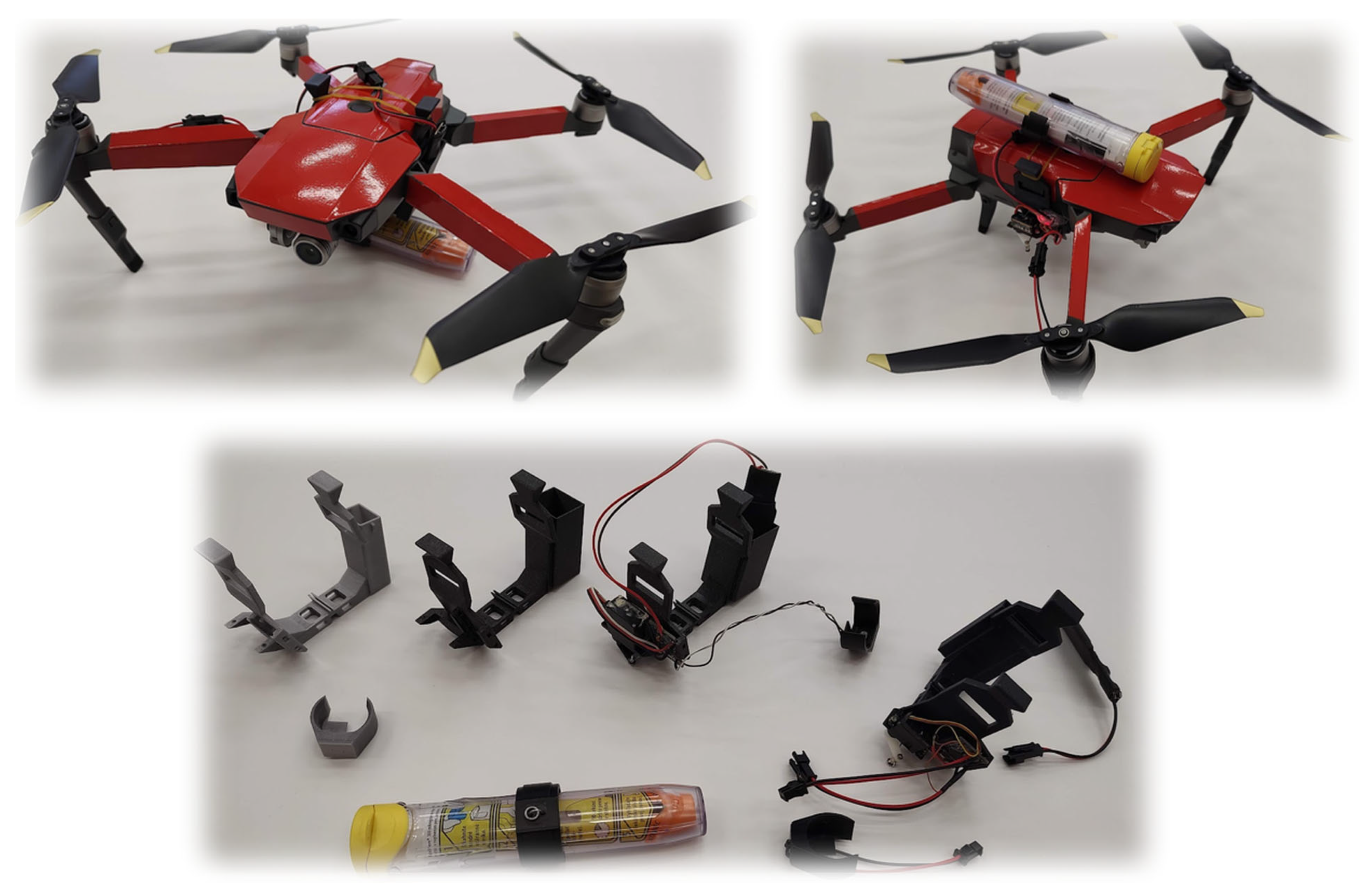
2.4. Mathematical Model of the Selected UAV

Taking into account the still-valid Slovak legislation that is unfavorable to autonomous flight and the flight of unmanned aerial vehicles beyond the line of sight (BVOLS), it is unprofitable for a company providing UAVs in the Slovak Republic to consider and implement a contract leading to the leasing of a specialized unmanned aerial vehicle from another foreign company providing UAVs/HEMS. Similarly, it is unprofitable to consider its design, construction, testing and homologation at one’s own expense without certainty regarding legislative changes and the possibility of using such a UAV in the territory of the Slovak Republic, in a protected area. By appropriately modifying the available multirotor unmanned aerial vehicle, a verification prototype will be created during initial testing to deliver and drop medications (for example, insulin, cardiovascular drugs or adrenaline pen) in difficult-to-reach mountainous terrain. Even such a seemingly simple additional service can relieve the HEMS operating in the High Tatras area to such an extent that it will be demonstrably relevant to invest in the development of one’s own unmanned aerial vehicle.

An important criterion when selecting a UAV suitable for modification to perform simple tasks related to medical use or to be used a supplementary rescue unmanned aerial vehicle is, in addition to the maximum take-off weight (maximum permitted payload), the type of unmanned aerial vehicle according to the support surfaces and the associated method of piloting the UAV.

Several different UAVs were considered for the modification of a conventional unmanned aerial vehicle into a supplementary rescue unmanned aerial vehicle. After deliberations and discussions with experts, the DJI Mavic Pro unmanned aerial vehicle was selected for initial testing purposes, the indisputable advantage of which is a sufficient payload capacity of up to 900 g in some scenarios and a UAV weight of less than 750 g; a flight speed-up to 65 km/h; a more than sufficient range of 7.5 km (15 km after firmware upgrade); and a flight time when using the maximum flight speed and optimal payload capacity exceeding 25 min (with upgraded batteries) [30]. Nevertheless, adding weight to the UAV affects its performance and other parameters, so these changes need to be carefully analyzed and balanced. Also, there is huge support for the modification of the UAV firmware and tools available. After this selection, we could proceed with the modelling of the UAV for the needs of the simulation environment.

A mathematical model of an UAV is essential for accurately predicting and optimizing its flight dynamics, control responses, and overall performance in various operational conditions. UAVs operate in complex and unpredictable environments, where factors such as aerodynamic forces, wind disturbances, and propulsion system behaviour directly influence their stability and maneuverability. Developing a rigorous mathematical representation allows engineers to simulate UAV behaviour under different flight scenarios without the risks and costs associated with real-world testing. Creating such a model requires the UAV’s physical and aerodynamic properties, including mass, center of gravity, moment of inertia, and airframe geometry, to be defined; this should be followed by the development of equations of motion that govern the aircraft’s translational and rotational dynamics. These equations incorporate external forces like air mass movement, gravity, lift, drag, and thrust, which are further refined through aerodynamic modelling based on wind tunnel data, empirical methods, or computational fluid dynamics (CFD) simulations. Additionally, the integration of control systems, such as PID controllers, state-space representations, or AI-based flight algorithms, ensures that UAVs can maintain stability and maneuverability. Furthermore, environmental factors, including turbulence, wind gusts, and temperature variations, must be incorporated alongside sensor fusion algorithms for accurate navigation and autonomous decision-making. Before real-world deployment, the final mathematical model is validated and fine-tuned through simulations in platforms like MATLAB-Simulink 2024b or ROS (Robot Operating System) [31]. Such models are crucial for improving the flight stability of UAVs, optimizing their fuel efficiency, enhancing their autonomy, and reducing their operational risks. By leveraging high-fidelity mathematical modelling, UAVs can be more reliable, efficient, and adaptable, particularly in challenging environments, including high-altitude mountain rescue operations and autonomous missions in adverse weather conditions.

The mathematical model of the selected unmanned aerial vehicle (UAV DJI Mavic Pro) must be considered for simulation purposes. A universal quadcopter model was developed based on general motion equations [32,33].

The complex motion of a UAV can be described by four fundamental movement components. These include changes in flight altitude, roll, pitch, and yaw. For general purposes and motion modelling, these can be simplified (the small angles are approximated, i.e., hover and near hover states, and the dynamics is linearized) and expressed as equations of a second-order system (1–3), as illustrated in Figure 8. For the rotation of the UAV around individual axes, we can state the following:

Roll (rotation around X-axis):

$$G_{roll}\left(s\right)={\displaystyle \frac{\varphi \left(s\right)}{{\tau }_{roll}\left(s\right)}}={\displaystyle \frac{K_{\varphi }}{J_x{s}^2+b_{x}s}}$$

(1)

Pitch (rotation around Y-axis):

$$G_{pitch}\left(s\right)={\displaystyle \frac{\theta \left(s\right)}{{\tau }_{pitch}\left(s\right)}}={\displaystyle \frac{K_{\theta }}{J_y{s}^2+b_{y}s}}$$

(2)

Yaw (rotation around Z-axis):

$$G_{yaw}\left(s\right)={\displaystyle \frac{\psi \left(s\right)}{{\tau }_{yaw}\left(s\right)}}={\displaystyle \frac{K_{\psi }}{J_z{s}^2+b_{z}s}}$$

(3)

where:

$\varphi$—is roll angle;

$\theta$—is pitch angle;

$\psi$—is yaw angle;

$\tau$—is input torques from motors;

$J_x; J_y; J_z$—is moment of inertia around each axis;

$b_x; b_y; b_z$—is damping coefficients;

$K_{\varphi }; K_{\theta }; K_{\psi }$—is torque-to-angle gain (depends on motor/thrust setup).

The translational dynamics (linear motion) of the UAV are described with the Equations (4)–(6), which relate net forces to positions along the body axes. For the X-direction (forward/backward, influenced by pitch), we can state the following:

$$G_x\left(s\right)={\displaystyle \frac{X\left(s\right)}{F_{pitch}\left(s\right)}}={\displaystyle \frac{K_x}{m{s}^2}}$$

(4)

For the Y-direction (left/right, influenced by roll), we can state the following:

$$G_y\left(s\right)={\displaystyle \frac{Y\left(s\right)}{F_{roll}\left(s\right)}}={\displaystyle \frac{K_y}{m{s}^2}}$$

(5)

For the Z-direction (Altitude, vertical thrust), we can write the following:

$$G_z\left(s\right)={\displaystyle \frac{Z\left(s\right)}{T\left(s\right)}}={\displaystyle \frac{K_z}{m{s}^2}}$$

(6)

where:

$m$—is the mass of the quadcopter;

$F$—is the net force generated from tilting;

$T$—is the total upward thrust;

$K_x; K_y; K_z—$is based on the gravity, motor force constants, and thrust-to-weight ratio.

The mathematical model of the UAV can be derived from the Equations (1)–(6), which describe the movement of the unmanned aerial vehicle along each axis in both the Earth coordinate system (X, Y, Z) and the UAV coordinate system (x, y, z). After obtaining the Equations of Motion and Kinematics for a Quadrotor UAV, defining the Coordinate Frames, and defining the orientation between them using Euler angles, we get a rotation matrix R (7), which defines the rotation from body frame to inertial frame. The position in the inertial frame is $p={\left[x,y,z\right]}^T$ and the linear velocity is $v=\dot{p}$. The rotation matrix R is then as follows:

$$\mathbf{R}=\left[\left.\begin{array}{ccc}{cos}_{\theta }{cos}_{\psi }& {sin}_{\varphi }{sin}_{\theta }{cos}_{\psi }-{cos}_{\varphi }{sin}_{\psi }& {cos}_{\varphi }{sin}_{\theta }{cos}_{\psi }+{sin}_{\varphi }{sin}_{\psi }\\ {cos}_{\theta }{sin}_{\psi }& {sin}_{\varphi }{sin}_{\theta }{sin}_{\psi }+{cos}_{\varphi }{cos}_{\psi }& {cos}_{\varphi }{sin}_{\theta }{sin}_{\psi }-{sin}_{\varphi }{cos}_{\psi }\\ {-s}_{\theta }& {sin}_{\varphi }{cos}_{\theta }& {cos}_{\varphi }{cos}_{\theta }\end{array}\right]\right.$$

(7)

If the angular velocity in body frame is defined as $\omega ={\left[p,q,r\right]}^T$, we can state the following (8), (9):

$$\left[\begin{array}{c}p\\ q\\ r\end{array}\right]=\mathbf{T}(\varphi ,\theta )\left[\begin{array}{c}\dot{\varphi }\\ \dot{\theta }\\ \dot{\psi }\end{array}\right]$$

(8)

$$\mathbf{T}\left(\varphi ,\theta \right)=\left[\begin{array}{ccc}1& 0& -\sin \theta \\ 0& \cos \varphi & \sin \varphi \cos \theta \\ 0& -\sin \varphi & \cos \varphi \cos \theta \end{array}\right]$$

(9)

The translational and rotational dynamic movement of the UAV can be described as follows (10):

$$m\ddot{p}=\mathbf{R}{\mathbf{F}}_T+{\mathbf{F}}_{wind}-mg\left[\begin{array}{c}0\\ 0\\ 1\end{array}\right]$$

(10)

where:

$m$—is the mass of the UAV;

$g$—is gravity;

${\mathbf{F}}_{T }$—is the thrust vector in the body frame;

${\mathbf{F}}_{wind}$—is the vector of the external force—as wind or turbulence;

$\tau$—is the torque vector.

And the total thrust from all four rotors for translational movement in the body z—direction is as follows (11):

$${\mathbf{F}}_T=\left[\begin{array}{c}0\\ 0\\ \mathsf{\Sigma }{T}_i\end{array}\right]$$

(11)

where:

${\mathbf{F}}_T$– is the total thrust from all four rotors in the body z-direction.

The rotational motion, using Euler’s rotational dynamics, can be written as follows (12):

$$\mathbf{I}\dot{\mathit{\omega }}+\mathit{\omega }\times \left(\mathbf{I}\mathit{\omega }\right)=\mathit{\tau }$$

(12)

where:

$\mathbf{I}$—is the moment of inertia matrix;

$\mathit{\tau }={\left[{\tau }_{\varphi }{\tau }_{\theta }{\tau }_{\psi }\right]}^T$—are the roll, pitch and yaw torques.

The thrust and torque from the rotors are described by $T_i=k_f{\omega }_i^2$ for thrust and ${\tau }_i=k_m{\omega }_i^2$ for torque. If the quadrotor is in “+” configuration, we can state the following (13):

$$\begin{array}{c}T=T_1+T_2+T_3+T_4\\ {\tau }_{\varphi }=l(T_2-T_4)\\ {\tau }_{\theta }=l(T_3-T_1)\\ {\tau }_{\psi }={\displaystyle \frac{k_m}{k_f}}(T_1-T_2+T_3-T_4)\end{array}$$

(13)

where:

$l$—is the distance from the center to the rotor;

${\omega }_i—$is the rotor angular velocity;

$k_f—$is the thrust coefficient;

$k_m$—is the moment coefficient.

The final System State Vector can be written as follows (14):

$$\mathbf{x}={\left[x,y,z,\varphi ,\theta ,\psi ,\dot{x,}\dot{y},\dot{z},p,q,r\right]}^T$$

(14)

The mathematical representation of the motion equations for the various flight phases of the unmanned aerial vehicle, in the studied and presented case of a quadcopter, together with the general motion equations of the quadcopter, form the foundation for developing a mathematical model for subsequent simulation purposes in the MATLAB-Simulink 2024b environment (Figure 9).

A mathematical model of the selected UAV (DJI Mavic Pro, which is modified into a supplementary UAV for HEMS purposes) serves as the foundation for simulations in the MATLAB-Simulink 2024b environment, enabling a precise analysis of flight dynamics, control algorithms, and environmental interactions before real-world deployment. Such supplementary UAVs operate in complex and unpredictable mountainous conditions, where factors such as aerodynamic forces, gravitational effects, wind disturbances, and thrust generation play a crucial role in flight stability and maneuverability.

The UAV model is formulated using Newton–Euler equations to accurately represent these specific dynamics, including translational and rotational motion. Furthermore, it incorporates forces such as gravity, aerodynamic lift and drag, thrust, and external environmental influences. These equations are implemented in MATLAB-Simulink 2024b as a system of differential equations, allowing real-time simulations of UAV behaviour under different operational conditions.

The MATLAB-Simulink 2024b simulation (Figure 9) consists of several interconnected functional blocks, each representing a critical component of UAV operations, including dynamics, control system, environmental interactions, and sensor feedback mechanisms. The Reference Input block provides the desired flight path or setpoint, such as altitude, velocity, or trajectory commands. Input is processed by the Controller, which could be a PID controller, state-space model, or model predictive control algorithm, generating appropriate control signals to maintain stability and ensure the UAV follows the intended trajectory. The Actuator Dynamics block models the propulsion system, servo motors, and thrust controllers, which convert these control signals into physical forces that affect UAV motion.

The UAV Dynamics block, based on Newton–Euler equations, governs the UAV’s movement, integrating external forces such as thrust, gravity, aerodynamic drag, and lift. Additionally, the Aerodynamics & Environmental Effects block simulates the impact of wind gusts, turbulence, and high-altitude atmospheric variations, which are especially critical in mountainous UAV operations where extreme weather fluctuations occur. The Sensors (IMU/GPS) block models real-world UAV navigation sensors, including an Inertial Measurement Unit (IMU), GPS, barometer, and magnetometer, which provide essential flight data and positioning accuracy. This sensor data is continuously fed back into the control system, forming a closed-loop feedback mechanism that dynamically adjusts UAV responses to optimize stability and flight performance.

Thanks to the integration of almost-real simulations in MATLAB-Simulink 2024b, researchers can softly tune crucial UAV parameters, test different control strategies, and validate mission-specific flight profiles. This simulation-based testing significantly reduces development costs, risks, and the need for extensive field trials. The ability to simulate realistic environmental conditions allows engineers to optimize UAVs for high-altitude or better mountainous applications such as search and rescue, environmental monitoring, and autonomous navigation in challenging terrains. As a result, MATLAB-Simulink 2024b is a suitable tool for advancing UAV technology, ensuring precision, efficiency, and reliability before UAVs are deployed in real-world scenarios. Moreover, MATLAB can be connected with additional third-party software, as will be discussed in the following subsections. This is the main reason we chose this environment as our simulation environment’s base.

3. Realization and Results of the Simulation Test Flights

It was essential to integrate a realistic environment into the simulation process to conduct high-fidelity UAV simulation flights that closely resemble real-world operations. This required the implementation of an accurate geographical representation of the determined area—The Little Cold Valley in the High Tatras.

Precise topographic scenery, with accurate geographic coordinates reflecting the current forestation levels, rocky terrain relief, infrastructure development, and built-up areas, can be obtained through paid services such as Elevation API, Google Earth or by integrating a highly detailed 3D environmental model. The execution of autonomous flight missions without direct pilot–operator input was also considered and implemented.

This was achieved by predefining flight waypoints, a method expected to be utilized in experimental real-world UAV flights as well. Establishing real-time interconnection and data communication between the specified software environments proved to be a key factor in the execution and evaluation of simulated UAV flights (Figure 10).

The following image (Figure 11) shows the final design of the simulation workplace for conducting simulated UAV flights in the determined area of The Little Cold Valley, integrated with the evaluation workstation for completed flights.

3.1. Evaluation of the Credibility and Success Rate of Simulated Flights

We subsequently used the workplace to simulate the flight of the selected UAV in a defined mountain environment (research area) for testing in order to verify the plausibility of the simulated scenarios and evaluate the success of the implementation of selected factors, such as weather, the influence of the mountain environment, signal loss, etc. The verification was performed using standardized tools such as Average Displacement Error (ADE), which provides an overall average error (15) between the predicted path and the actual path over the entire flight [34,35,36]:

$$\mathrm{A}\mathrm{D}\mathrm{E}={\displaystyle \frac{1}{T}}\sum _{t=1}^T‖p_{pr}\left(t\right)-p_{tr}\left(t\right)‖$$

(15)

where:

$t$—is the time;

$T$—is the total number of timesteps;

$p_{pr}\left(t\right)$—is the predicted or planned UAV position at time $t$;

$p_{tr}\left(t\right)$—is the actual or ground truth UAV position at time $t$.

The Final Displacement Error (FDE) provides information about the error (distance) between the UAV’s predicted final position and its actual final position (16):

$$\mathrm{F}\mathrm{D}\mathrm{E}=‖p_{pr}\left(T\right)-p_{tr}\left(T\right)‖$$

(16)

where:

$T$—is the final time step;

$p_{pr}\left(t\right)$—is the predicted (or planned) UAV position at the final time step $T$;

$p_{tr}\left(t\right)$—is the actual (or true) UAV position at the same final time step $T$.

In a mountainous environment with challenging updrafts, uneven terrain and potential GPS errors, the above-mentioned metrics helps evaluate how well the path planner or controller performed over time and at the end of the flight in the two-dimensional environment; thus, we also needed to adapt the metrics to the three-dimensional environment (17):

$$\mathrm{F}\mathrm{D}\mathrm{E}=\sqrt{{\left(x_{pr}\right(t)-x_{tr}(t\left)\right)}^2+{\left(y_{pr}\right(t)-y_{tr}(t\left)\right)}^2+{\left(z_{pr}\right(t)-z_{tr}(t\left)\right)}^2}$$

(17)

where:

${x, y,z }_{pr}$—are predicted coordinates of the UAV;

$x,{y,z }_{tr}$—are the real coordinates of the UAV.

After obtaining the evaluation metrics, we proceeded to perform simulated flights in the complex simulation workplace with the selected and modelled UAV (Figure 12).

After the verification of the simulation workplace with simulated flights, we proceeded to verify the influences of weather and GNSS signal deterioration in four model scenarios (S1–S4), where scenario S1 represents flights in good atmospheric conditions (sunny weather with low to very moderate winds), scenario S2 represents slightly deteriorated conditions, namely moderate cloud cover and wind gusts, scenario S3 represents a flight over steep terrain with the presence of relatively large altitude drops, and scenario S4 represents flights in sunny weather but with the presence of significant turbulence. These scenarios were chosen purposely for the testing of the simulation workplace as they represent four idealized scenarios for the delivery of medicament to the high mountain environment. A successful delivery is a delivery anywhere inside the determined area—a circle with a 5 m diameter [11]. Also, an ideal path with safe corridor limits was set in the simulations (Figure 12).

The difference between the ideal flight path parameters and parameters affected by weather and other external influences (Figure 13) was evaluated by standard metrics (16–18) to obtain the Average Displacement Error (ADE) and Final Displacement Error (FDE). The outcome of this comparison is shown in

Table 3. The evaluation table.

Scenario	Flight Conditions	ADE	FDE	Remarks
S1	Ideal meteorological conditions Good visibility during the day Sunny Low Wind	0.73 m	1.14 m	Observed good correlation.
S2	Favorable meteorological conditions Reduced visibility in the evening Moderate Wind GNSS multipath error	1.18 m	2.03 m	Larger deviation—wind gusts caused variation in flight.
S3	Adverse meteorological conditions Heavy rain Strong wind gusts Reduced daytime visibility	1.49 m	2.97 m	Performance impacted by abrupt altitude changes. Moderate offsets due to slight GPS drift
S4	Adverse meteorological conditions Snowfall (without icing), Reduced daytime visibility GNSS multipath error	2.14 m	4.12 m	Significant difference at final waypoints due to large wind disturbances. Major offsets due to GPS drift

.

All the simulation flights were performed on a computer with an Intel i7-14700hx processor, 32 GB of RAM and a Nvidia GeForce RTX4070 graphic card, using Windows 11 and MATLAB-Simulink version 2024b. After verification, we can state that the Average Displacement Error was lowest in scenario S1 and highest in scenario S4. The Final Displacement Error was also lowest in scenario S1 and highest in scenario S4. This outcome correlates with our initial expectations [10,11]. Also, the ADE and FDE were in the desired range (within the circle with a 5 m diameter), and we can state that the simulation workplace is suitable for the needs of our research team and for demonstration purposes, both for the Civil Aviation Authorities of the Slovak Republic and for the Air Rescue Services. The simulation workplace can also be used to train potential UAV operators as it can be supplemented with metrics for UAV operator skill evaluation.

3.2. The Ablation Study

Using the simulation workplace described in Chapter 2, we started from the baseline of Scenario S1—ideal daylight conditions, low wind, unobscured GNSS, and flat-plate guidance—which yielded a mean Average Displacement Error (ADE) of 0.73 m and a Final Displacement Error (FDE) of 1.14 m. We then re-ran the same flight profile thirty times per condition, but activated only one disturbance factor at a time while keeping all other parameters identical. Random seeds for atmospheric turbulence and sensor noise were changed between runs to obtain statistically stable means (n = 30.95% confidence). The outcomes (

Table 4. The quantitative outcomes of the ablation study.

Disturbance Factor (Single Ablation)	Mean ADE ± σ [m]	ΔADE vs. Baseline [m]	Mean FDE ± σ [m]	ΔFDE vs. Baseline [m]	%-Increase in FDE
Baseline (S1)	0.73 ± 0.03	–	1.14 ± 0.05	–	–
Moderate steady wind (5 m/s)	1.05 ± 0.06	+0.32	1.58 ± 0.12	+0.44	+39%
Wind gusts (5–10 m/s, 0.5 Hz)	1.35 ± 0.09	+0.62	2.22 ± 0.18	+1.08	+95%
GNSS multipath (C/N0 drop 8 dB)	1.00 ± 0.04	+0.27	1.62 ± 0.13	+0.48	+42%
Steep-terrain climb (600 m relief)	1.12 ± 0.05	+0.39	1.95 ± 0.15	+0.81	+71%
Heavy rain (12 mm/h)	1.15 ± 0.05	+0.42	1.82 ± 0.14	+0.68	+60%
Snowfall (wet snow, 2 mm/h)	1.28 ± 0.07	+0.55	2.05 ± 0.16	+0.91	+80%
Mountain-wave turbulence (±6 m/s)	1.52 ± 0.11	+0.79	2.95 ± 0.22	+1.81	+159%

) can be defined as follows:

• Turbulence dominated the error budget. Mountain-wave vertical velocities produced the most significant displacement, almost tripling the FDE. Control bandwidth limits rather than raw thrust explained most of the excursion.
• Wind magnitude mattered more than precipitation. A shift from a steady breeze to gusts doubled the terminal error, whereas adding heavy rain increased the FDE by only ~0.7 m. Aerodynamic coupling between roll commands and lateral gusts was the principal mechanism.
• Sensor-induced errors were secondary but non-negligible. The GNSS multipath alone increased the FDE by 0.48 m and occasionally triggered short-lived autonomous hover modes. When turbulence and multipath were combined in exploratory dual-factor runs, the effects were roughly additive, confirming a weak interaction.
• Topography affected guidance loops more than aerodynamics. The steep-terrain ablation necessitated aggressive climb power-sharing; energy management limits extended the flight path and increased the FDE by 0.81 m.
• Expressed as Cohen’s d (factor mean—baseline mean divided by pooled σ), turbulence yielded an FDE of d ≈ 15—a huge effect—whereas GNSS multipath gave d ≈ 4. All other single factors fell between these extremes, indicating that mitigations should prioritize real-time turbulence sensing and adaptive trajectory smoothing.

The ablation study isolated and quantified the relative contributions of seven disturbance mechanisms to the path-tracking accuracy. Turbulence and wind gusts posed the most significant single-factor threats, suggesting that mountain rescue UAVs will benefit most from rapid response attitude controllers and onboard micro-doppler turbulence radars, whereas further GNSS hardening provides diminishing returns unless combined with inertial navigation upgrades.

4. Discussion

The presented research results demonstrate the feasibility of using a dedicated high-altitude UAV simulation environment to enhance flight performance and operational safety in mountainous environments. The proposed simulation workplace integrates real-time weather modelling, terrain analysis, and UAV flight dynamics to provide a realistic and adaptable environment for testing UAVs under extreme meteorological conditions. The MATLAB-Simulink MATLAB-Simulink 2024b toolboxes provided us with the ability to simulate aerodynamic and environmental effects, such as wind gusts, turbulence, and high-altitude atmospheric variations. Even though our complex simulation workplace was primarily tested in a specific region—The Little Cold Valley in the High Tatras, Slovakia—the Elevation API (or DTED dataset import), together with the Weather API by Meteomatics, could extend the complex simulation workplace to another desired area.

Previous studies have explored UAV applications in complex environments, including mountainous regions. However, few have focused on a comprehensive simulation framework that integrates meteorological variability, real-time flight dynamics, and terrain-specific challenges. For example, we can mention a study investigating UAV-based snow depth mapping in alpine regions and highlighting the importance of accurate environmental modelling for flight stability and data collection. However, this study primarily focused on static UAV flight conditions. In contrast, the present research incorporates dynamic weather conditions such as wind gusts, turbulence, and air density fluctuations, which are critical for UAV maneuverability and control [37]. The same research examined UAV applications for environmental monitoring in mountainous areas, emphasizing the need for high-resolution geospatial modelling. These studies relied on UAV-LiDAR data to assess terrain interactions; our simulation framework extends beyond terrain mapping via integrating atmospheric modelling and real-time meteorological data, offering a more comprehensive means of performing UAV flight simulation in high-altitude conditions [38,39]. Next, a UAV simulation model developed in MATLAB-Simulink 2024b for debris flow and topographic analysis can be mentioned. However, it did not incorporate stochastic wind turbulence models or high-altitude atmospheric effects. In contrast, our study advances UAV flight simulation by embedding real-time adaptive flight path optimization based on weather prediction models, enhancing UAV stability and reliability in unpredictable conditions [40,41]. Moreover, the subsequent study explored avalanche hazard assessment using UAVs but did not include a pre-flight simulation component, which is critical for ensuring UAV safety before deployment. The following example is a study that analyzed UAV applications for landslide monitoring and grassland changes in Central Asia; these studies lacked a dedicated simulation component for high-altitude environments [42,43,44]. Our presented study aligns more closely with a study which integrated UAV photogrammetry for rock slope stability analysis [45]. However, we extend their work by incorporating full-scale UAV operational simulations for medical and rescue applications, ensuring UAVs can perform under extreme atmospheric disturbances.

Simulating UAV behaviour in high-mountain regions allows for better mission planning, improved pilot training, and enhanced UAV adaptability in disaster response scenarios. Nevertheless, certain limitations remain. The simulation does not fully replicate microclimatic variations, such as sudden downdrafts or localized wind shear, requiring higher-resolution atmospheric modelling. Incoming research should focus on refining meteorological simulations with machine learning algorithms for real-time adaptive control during UAV operations. Additionally, validation through real-world UAV flight data will further enhance the reliability of the simulation framework.

While advanced simulation environments enable the rigorous testing and optimization of UAV automatic flight route selection, there remain significant distinctions from real-time operations that must be acknowledged. Simulations, even when integrating real-time weather and high-resolution terrain data, cannot fully capture the unpredictability of real-world environments, such as microclimatic changes, sensor failures, or sudden obstacles. Additionally, real-world operations involve regulatory constraints, communication delays, and unforeseen risks that simulations often idealize or omit. As a result, automatic route selection validated solely in simulation may overlook crucial operational hazards, resulting in routes that are less robust or even unsafe when deployed in practice. Therefore, bridging the gap between simulated and real-world UAV operations requires the cautious interpretation of simulation results, incremental field validation, and the integration of conservative safety margins to ensure that automated flight planning performs reliably under the complexities of actual flight conditions.

Compared to existing studies, this research significantly enhances UAV flight simulation by integrating real-time weather modelling and terrain-specific flight analysis. These advancements position the proposed simulation workplace as a robust testing platform for UAV applications in extreme environments, paving the way for future developments in remotely controlled or autonomous aerial rescue operations.

5. Conclusions

This research has established and validated a sophisticated simulation environment for UAV-assisted life-saving operations in a mountainous terrain, specifically addressing the complex meteorological and topographical challenges of the High Tatras in Slovakia. It integrates high-resolution real-time weather and elevation data with detailed UAV dynamic models within MATLAB-Simulink 2024b. With interoperability within simulation platforms such as Prepar3D v6.1, we have demonstrated that simulated UAV missions can reliably predict operational performance under adverse conditions, with the delivery accuracies being within predefined ranges. The conducted ablation studies examined the impact of selected parameters, including turbulence, wind gusts, and GNSS signal deterioration, on flight path accuracy, which helped identify critical technical priorities for the future development of UAVs and their control systems. Our goal is to create and provide a reliable, safe, and cost-effective simulation workplace for operator training, financial analysis, and the development and deployment of different UAVs in mountain rescue and emergency medical service (HEMS) scenarios. We would also like to create a risk-mitigating platform for mission planning, operator training, and, ultimately, a tool for future regulatory discourse. To ensure the simulation’s fidelity and its translation to real-world practice, field validation through empirical UAV test flights remains essential, particularly for capturing microclimatic and unpredictable environmental factors. Unfortunately, the Slovak authorities and legislation do not currently allow us to perform flights in the desired area of research—Little Cold Walley in the High Tatras. In future research, we envision the expansion of our solution (modular simulation architecture) to other geographies with varying terrains and climates, incorporating higher-resolution and machine-learning-enhanced atmospheric modelling and enabling fleet-level multi-agent operations. Such complex simulation environments, based on a modular conception, could serve as a foundation for regulatory and economic assessments, potentially leading to the better adoption and operational integration of UAVs into diverse and challenging rescue environments. We also plan to incorporate different UAV models (types), such as UAVs for medication delivery, UAVs for the delivery of goods (food, water, emergency equipment), or UAVs equipped with sensors for search and rescue mission planning purposes (FLIR, Thermal vision, etc.), and the AI logic that will choose the best UAV for each mission type considering the different conditions, like the actual weather, GNSS deterioration in the area of the interest and of course the limitations of the pilot–operator of the UAV. The future integration of real-time meteorological simulations and flight optimization in our study may provide a cost-effective alternative to field trials while reducing the risks associated with unpredictable weather patterns.

References

1. Naidoo, Y.; Stopforth, R.; Bright, G. Development of an UAV for search & rescue applications. In Proceedings of the IEEE Africon ’11, Victoria Falls, Zambia, 13–15 September 2011; pp. 1–6. [Google Scholar] [CrossRef]
2. Liu, Z.; Chen, H.; Wen, Y.; Xiao, C.; Chen, Y.; Sui, Z. Mode Design and Experiment of Unmanned Aerial Vehicle Search and Rescue in Inland Waters. In Proceedings of the 6th International Conference on Transportation Information and Safety (ICTIS), Wuhan, China, 22–24 October 2021; pp. 917–922. [Google Scholar] [CrossRef]
3. Jin, Z.; Nie, L.; Li, D.; Tu, Z.; Xiang, J. An Autonomous Control Framework of Unmanned Helicopter Operations for Low-Altitude Flight in Mountainous Terrains. Drones 2022, 6, 150. [Google Scholar] [CrossRef]
4. Rudol, P.; Doherty, P. Human Body Detection and Geolocalization for UAV Search and Rescue Missions Using Color and Thermal Imagery. In Proceedings of the 2008 IEEE Aerospace Conference, Big Sky, MT, USA, 1–8 March 2008; pp. 1–8. [Google Scholar] [CrossRef]
5. ter Avest, E.; Kratz, M.; Dill, T.; Palmer, M. HEMS in mountain and remote areas: Reduction of carbon footprint through drones? Scand. J. Trauma. Resusc. Emerg. Med. 2023, 31, 36. [Google Scholar] [CrossRef] [PubMed]
6. Claesson, A.; Fredman, D.; Svensson, L. Unmanned aerial vehicles (drones) in out-of-hospital-cardiac-arrest. Scand. J. Trauma. Resusc. Emerg. Med. 2016, 24, 124. [Google Scholar] [CrossRef]
7. Ozbiltekin-Pala, M.; Yavas, V.; Ozkan-Ozen, Y.D. Drivers and barriers of unmanned aerial vehicles in emergency logistics operations. Technol. Soc. 2025, 82, 102894. [Google Scholar] [CrossRef]
8. Eskandaripour, H.; Boldsaikhan, E. Last-Mile Drone Delivery: Past, Present, and Future. Drones 2023, 7, 77. [Google Scholar] [CrossRef]
9. Elmeseiry, N.; Alshaer, N.; Ismail, T. A Detailed Survey and Future Directions of Unmanned Aerial Vehicles (UAVs) with Potential Applications. Aerospace 2021, 8, 363. [Google Scholar] [CrossRef]
10. Češkovič, M.; Kurdel, P.; Gecejová, N.; Labun, J.; Gamcová, M.; Lehocký, M. A Reasonable Alternative System for Searching UAVs in the Local Area. Sensors 2022, 22, 3122. [Google Scholar] [CrossRef]
11. Kurdel, P.; Gecejová, N.; Češkovič, M.; Yakovlieva, A. Evaluation of the Success of Simulation of the Unmanned Aerial Vehicle Precision Landing Provided by a Newly Designed System for Precision Landing in a Mountainous Area. Aerospace 2024, 11, 82. [Google Scholar] [CrossRef]
12. Gecejová, N.; Češkovič, M.; Kurdel, P.; Kopyt, A. Simulation and Analysis of the Change in the Radiation Characteristics of the Communication and Telemetry Antenna of the UAV Used as a Supplementary Rescue Device for SAR and HEMS. In Proceedings of the New Trends in Aviation Development 2023: The XVIII International Scientific Conference, New York, NY, USA, 20–22 September 2023; Institute of Electrical and Electronics Engineers: New York, NY, USA, 2023; pp. 71–76, ISBN 979-8-3503-7040-9. [Google Scholar] [CrossRef]
13. Biliderov, S.; Kamenov, K.; Calovska, R.; Georgiev, G. Synthesis and Testing of an Algorithm for Autonomous Landing of a UAV under Turbulence, Wind Disturbance and Sensor Noise. Eng. Proc. 2024, 70, 41. [Google Scholar] [CrossRef]
14. Polishchuk, V.; Kelemen, M.; Kelemen, M.; Polishchuk, A.; Gasparović, G. Unmanned Aerial Vehicle Flight Risk Assessment Model for Environmental Research on Mountain Terrain. In Proceedings of the 2021 6th International Conference on Smart and Sustainable Technologies (SpliTech), Bol and Split, Croatia, 8–11 September 2021; pp. 1–5. [Google Scholar] [CrossRef]
15. Zhang, M.; Han, Y.; Chen, S.; Liu, M.; He, Z.; Pan, N. A Multi-Strategy Improved Differential Evolution Algorithm for UAV 3D Trajectory Planning in Complex Mountainous Environments. Eng. Appl. Artif. Intell. 2023, 125, 106672. [Google Scholar] [CrossRef]
16. Bremer, M.; Wichmann, V.; Rutzinger, M.; Zieher, T.; Pfeiffer, J. Simulating Unmanned-Aerial-Vehicle Based Laser Scanning Data for Efficient Mission Planning in Complex Terrain. ISPRS Arch. 2019, XLII-2/W13, 943–950. Available online: https://isprs-archives.copernicus.org/articles/XLII-2-W13/943/2019/ (accessed on 1 March 2025).
17. Barton, J.D.; Cybyk, B.; Drewry, D.G.; Frey, T.M.; Funk, B.K.; Hawthorne, R.C.; Keane, J.F. Use of a High-Fidelity UAS Simulation for Design, Testing, Training, and Mission Planning for Operation in Complex Environments. Encycl. Remote Sens. 2010, 1–14. [Google Scholar] [CrossRef]
18. Shi, Z.; Zhang, J.; Shi, G.; Ji, L.; Wang, D.; Wu, Y. Design of a UAV Trajectory Prediction System Based on Multi-Flight Modes. Drones 2024, 8, 255. [Google Scholar] [CrossRef]
19. Wang, W.; Xiong, W.; Ouyang, X.; Chen, L. TPTrans: Vessel Trajectory Prediction Model Based on Transformer Using AIS Data. ISPRS Int. J. Geo-Inf. 2024, 13, 400. [Google Scholar] [CrossRef]
20. Kovanič, Ľ.; Blistan, P.; Urban, R.; Štroner, M.; Blišťanová, M.; Bartoš, K.; Pukanská, K. Analysis of the Suitability of High-Resolution DEM Obtained Using ALS and UAS (SfM) for the Identification of Changes and Monitoring the Development of Selected Geohazards in the Alpine Environment—A Case Study in High Tatras, Slovakia. Remote Sens. 2020, 12, 3901. [Google Scholar] [CrossRef]
21. Meier, K.; Hann, R.; Skaloud, J.; Garreau, A. Wind Estimation with Multirotor UAVs. Atmosphere 2022, 13, 551. [Google Scholar] [CrossRef]
22. Lei, Y.; Li, Y.; Wang, J. Aerodynamic Analysis of an Orthogonal Octorotor UAV Considering Horizontal Wind Disturbance. Aerospace 2023, 10, 525. [Google Scholar] [CrossRef]
23. Meteomatics. Weather API. Available online: https://www.meteomatics.com/en/weather-api/ (accessed on 14 November 2024).
24. Li, W.; Cui, S.; Zhao, J.; An, L.; Yu, C.; Ding, Y.; Jing, H.; Liu, Q. Experimental Study of Wind Characteristics at a Bridge Site in Mountain Valley Considering the Effect of Oncoming Wind Speed. Appl. Sci. 2024, 14, 10588. [Google Scholar] [CrossRef]
25. Pandharinath, N. Aviation Meteorology; Himalaya Publishing House: Mumbai, India, 2014; ISBN 9789386211361. [Google Scholar]
26. International Electrotechnical Commission (IEC). IEC 60529/A1:1999 Degrees of Protection Provided by Enclosures (IP Code)—Amendment 1; IEC: Geneva, Switzerland, 1999. [Google Scholar]
27. Slovak Office of Standards, Metrology and Testing. Degrees of Protection Provided by Enclosures (IP Code); STN EN 60529/A1:2002 (33 0330); ÚNMS SR: Bratislava, Slovakia, 2002. [Google Scholar]
28. Google Developers. Elevation API Overview. Available online: https://developers.google.com/maps/documentation/elevation/overview (accessed on 1 December 2024).
29. Gecejová, N.; Češkovič, M.; Yakovlieva, A. Concept of the Alternative Protection of the High and Very High-Voltage Power Lines During Flights of the Conventional Aircraft and Unmanned Aerial Vehicles. In Proceedings of the IEEE 9th International Conference on Energy Smart Systems (ESS), Kyiv, Ukraine, 29–31 October 2024. [Google Scholar]
30. DJI. Mavic Pro User Manual, V2.0. Available online: https://dl.djicdn.com/downloads/mavic/20171219/Mavic%20Pro%20User%20Manual%20V2.0.pdf (accessed on 20 February 2025).
31. Ahmed, A.H.; Ouda, A.N.; Kamel, A.M.; Elhalwagy, Y.Z. Design and Analysis of Quadcopter Classical Controller. In Proceedings of the 16th International Conference on Aerospace Sciences & Aviation Technology (ASAT-16), Cairo, Egypt, 26–28 May 2015; Military Technical College: Cairo, Egypt, 2015. [Google Scholar]
32. Cárdenas, C.A.; Grisales, V.H.; Collazos Morales, C.A. Quadrotor Modeling and a PID Control Approach. In Intelligent Human Computer Interaction; Lecture Notes in Computer Science; Springer: Cham, Switzerland, 2020; pp. 281–291. [Google Scholar] [CrossRef]
33. Carlone, L.; Ryll, M. Visual Navigation for Autonomous Vehicles (VNAV); Lecture 6: Quadrotor Dynamics. Fall 2023. Available online: https://wilselby.com/research/arducopter/model-verification/ (accessed on 18 February 2025).
34. Xu, K.; Qin, Z.; Wang, G.; Huang, K.; Ye, S.; Zhang, H. Collision-Free LSTM for Human Trajectory Prediction. In Proceedings of the International Conference on Multimedia Modeling, Bangkok, Thailand, 5–7 February 2018; Springer: Cham, Switzerland, 2018; pp. 106–116. [Google Scholar]
35. Alahi, A.; Goel, K.; Ramanathan, V.; Robicquet, A.; Fei-Fei, L.; Savarese, S. Social LSTM: Human Trajectory Prediction in Crowded Spaces. In Proceedings of the IEEE Conference on Computer Vision and Pattern Recognition (CVPR), Las Vegas, NV, USA, 27–30 June 2016; IEEE: Piscataway, NJ, USA, 2016; pp. 961–971. [Google Scholar]
36. Zhang, H.; Goodfellow, I.; Metaxas, D.; Odena, A. Self-Attention Generative Adversarial Networks. In Proceedings of the International Conference on Machine Learning, Long Beach, CA, USA, 9–15 June 2019; PMLR: New York, NY, USA, 2019; pp. 7354–7363. [Google Scholar]
37. Revuelto, J.; Alonso-Gonzalez, E.; Vidaller-Gayan, I. Intercomparison of UAV Platforms for Mapping Snow Depth Distribution in Complex Alpine Terrain. Cold Reg. Sci. Technol. 2021, 186, 103282. [Google Scholar] [CrossRef]
38. Tomczyk, A.M.; Ewertowski, M.W.; Creany, N. The application of unmanned aerial vehicle (UAV) surveys and GIS to the analysis and monitoring of recreational trail conditions. Int. J. Appl. Earth Obs. Geoinf. 2023, 123, 103474. [Google Scholar] [CrossRef]
39. Feng, T.; Hao, X.; Wang, J.; Luo, S.; Huang, G.; Li, H.; Zhao, Q. Applicability of alpine snow depth estimation based on multitemporal UAV-LiDAR data: A case study in the Maxian Mountains, Northwest China. J. Hydrol. 2023, 617, 129006. [Google Scholar] [CrossRef]
40. Dhote, P.R.; Thakur, P.K.; Chouksey, A.; Srivastav, S.K.; Raghvendra, S.; Rautela, P.; Ranjan, R.; Allen, S.; Stoffel, M.; Bisht, S.; et al. Synergistic analysis of satellite, unmanned aerial vehicle, terrestrial laser scanner data and process-based modelling for understanding the dynamics and morphological changes around the snout of Gangotri Glacier, India. Geomorphology 2022, 396, 108005. [Google Scholar] [CrossRef]
41. Ramirez, R.A.; Kwon, T.H. UAV-LiDAR System Development for High-Resolution Topographic Analysis in Forest Environments. Heliyon 2023, 9, e15208. [Google Scholar] [CrossRef]
42. Denissova, N.; Petrova, O.; Mashayev, E.; Spivak, D.; Zuyev, V.; Daumova, G. Real-Time Avalanche Hazard Monitoring System Based on Weather Sensors and a Laser Rangefinder. Sensors 2025, 25, 2937. [Google Scholar] [CrossRef]
43. Jiang, N.; Zhou, J.; Li, C.; Li, H. A Landslide Monitoring Method Using Data from UAV and Terrestrial Laser Scanning with Insufficient and Inaccurate Ground Control Points. J. Rock Mech. Geotech. Eng. 2024, 16, 344–358. [Google Scholar] [CrossRef]
44. Qiu, C.; Zhang, C.; Ma, J.; Yang, C.; Wang, J.; Mandakh, U.; Ganbat, D.; Myanganbuu, N. Analysis of Grassland Vegetation Coverage Changes and Driving Factors in China–Mongolia–Russia Economic Corridor from 2000 to 2023 Based on RF and BFAST Algorithm. Remote Sens. 2025, 17, 1334. [Google Scholar] [CrossRef]
45. Safuan, A.R.A.; Sa’ari, R.; Mustaffar, M. Integration of TLS and UAV Digital Photogrammetry for Rock Slope Stability Analysis. Measurement 2022, 203, 112074. [Google Scholar] [CrossRef]
Figure 1. Example of modified UAV (with drop option) as a supplementary means of drug delivery during life-saving missions. The drop system together with EpiPen weighs only 120 g.
Drones 09 00416 g001
Figure 2. The simulation workplace in MATLAB-Simulink 2024b interconnected with Prepar3D v6.1 via Simconnect.
Drones 09 00416 g002
Figure 3. Example of historical, current and forecast weather development on the route from ATE Station in Poprad Airport (LZTT) to Zamkovského Chalet, imported via Weather API to the simulation environment. The blue course represents the temperature change forecast, the green course represents the wind speed forecast, and the magenta course represents the precipitation forecast.
Drones 09 00416 g003
Figure 4. The MATLAB-Simulink 2024b simulation of the GNSS signal deterioration caused by multipath propagation error and the blocking of the visible satellites caused by surrounding hills, implemented in the complex simulation workplace.
Drones 09 00416 g004
Figure 5. Comprehensive simulation workplace integration with MATLAB-Simulink 2024b, Prepar3D v6.1, Elevation API and Weather API by Meteomatics, interconnected by SimConnect.
Drones 09 00416 g005
Figure 6. SimConnect round-trip latency evaluation during testing. The dotted line represents the acceptance criteria threshold.
Drones 09 00416 g006
Figure 7. Example of simulation workplace outputs—visual demonstration of meteorological phenomena effects in the determined environment (on the left: the lower station of the Hrebienok funicular; on the right: the hiking trail to Zamkovského Chalet, passing through the main section of The Little Cold Valley in the High Tatras). Legend: (a) Ideal meteorological conditions—good visibility during the day; (b) Favorable meteorological conditions—reduced visibility in the evening; (c) Adverse meteorological conditions—heavy rain accompanied by strong wind gusts, and reduced daytime visibility; (d) Adverse meteorological conditions—snowfall and reduced daytime visibility.
Drones 09 00416 g007
Figure 8. Representation of the movement and rotation axes of the unmanned aerial vehicle—quadcopter.
Drones 09 00416 g008
Figure 9. Illustration of UAV mathematical model created in MATLAB-Simulink 2024b.
Drones 09 00416 g009
Figure 10. Simulated flight of the modified UAV Mavic Pro from Poprad–Tatry Airport (LZTT) HEMS station to the rescue site at Zamkovského Chalet, The Little Cold Valley—graphical representation of the simulation-derived data.
Drones 09 00416 g010
Figure 11. Actual design of the simulation workplace for UAV flight simulations in the designated area of The Little Cold Valley.
Drones 09 00416 g011
Figure 12. Complex simulation workplace used for testing UAV flight scenario.
Drones 09 00416 g012
Figure 13. Simulated UAV flight scenario (affected by weather influences and GNSS signals deterioration) evaluation.
Drones 09 00416 g013