A Consensus Control Method for Unmanned Aerial Vehicle (UAV) Swarm Based on Molecular Dynamics

Abstract

In the field of unmanned aerial vehicle (UAV) swarm control, achieving efficient consensus is paramount. This paper proposes a molecular dynamics-based UAV swarm consensus control strategy. The strategy emulates the random motion of molecules in a vacuum, establishing a framework for UAV swarm behavior that aligns with principles from molecular dynamics. The framework is built upon the Vicsek model, a cornerstone in swarm dynamics, and employs the Lennard-Jones and Morse potential functions to model the attractive and repulsive forces between UAVs. Through simulation, this paper explores how different potential functions and swarm sizes affect consensus control, finding the Morse potential particularly advantageous. Theoretical analysis and experimental results demonstrate that these potential functions not only prevent UAV collisions but also facilitate the emergence of swarming behaviors, thereby enhancing the collaborative efficiency and stability of UAV swarms. This advancement significantly boosts the overall performance of swarm control, paving the way for the deployment of UAV swarms in complex environments.

1. Introduction

The objective of cooperative control of multi-agent systems is to enable multiple agents to collaborate under specific conditions, thereby optimizing overall system performance [1]. This has attracted extensive research from numerous scientists, encompassing areas such as cooperative control, formation control, flocking control, distributed sensor networks, and satellite cluster attitude alignment, among others [2,3,4,5,6,7]. Particularly in multi-agent systems, the dynamic behavior of each agent is influenced by the others, necessitating the consideration of inter-agent relationships and interactions to achieve the distributed cooperative control of a UAV swarm.

In nature, flocking refers to the collective movement behavior of a large number of biological individuals forming a biological community, which emerges from local information exchange and follows simple rules to exhibit global, complex behavior [8,9]. This phenomenon is observed in various contexts, such as bird migration and fish swimming in coordinated patterns, and is commonly referred to as “flocking behavior”. Flocking specifically describes the movement of a large number of autonomous individuals in space all moving in the same direction at a consistent speed while maintaining a constant distance from one another, voiding both separation and collision [10]. The primary objective is to achieve a predefined desired distance between neighboring agents while also ensuring that all agents converge to a uniform speed without requiring a fixed topology. Current research focuses on enhancing the efficiency, robustness, and adaptability of algorithms, as well as addressing challenges related to communication limitations and dynamic environments.

The research on flocking control can be traced back to 1987, when Reynolds utilized three fundamental principles observed in biological groups, repulsion, cohesion, and alignment, to computationally simulate the dynamics of collective behavior, resulting in the seminal Boid model [11]. This model has since been widely embraced and utilized as a foundational framework, where the velocities, sizes, and directions of individuals within a flock tend to stabilize into a consistent state over time. Expanding on Reynolds’ work, Hungarian scientist Vicsek [12] proposed the Vicsek model, which describes how individuals align their movements based on the average direction of their neighbors. Subsequently, researchers have used various mathematical tools for rigorous theoretical analysis and modeling of flocking control, such as graph theory and stability theory, to demonstrate the stability and convergence of the system. In 2004, Olfati-Saber et al. [13] successfully summarized the communication topological relationships between agents as a network communication topological graph by analyzing a first-order dynamic model problem with time delay and changing topology. This provided a geometric or geometrical interpretation of the three rules of flocking behavior. This method laid the foundation for consensus control theory.

In recent years, extensive research has been conducted globally on consensus control for unmanned aerial vehicle (UAV) swarms. This field focuses on enabling multi-agent systems to exhibit collective behaviors and maintain coherent formations [14,15]. To tackle the associated challenges, researchers have pursued diverse methodologies, which can be broadly categorized as follows: 1. Distributed control based on graph theory. Graph theory is used to describe the communication topology among UAVs, and consensus protocols are designed to achieve state synchronization. Wang proposed a multi-layer graph model to improve the scalability of the network topology in large-scale swarms and designed a multi-layer recursive consensus control concept to achieve consensus among UAVs [16]. 2. Bio-inspired algorithms. Drawing inspiration from natural collective behaviors such as bird flocking and fish schooling, methods like the Boid model achieve self-organized coordination through separation, alignment, and cohesion rules. Guo [17] introduced a distributed flocking control strategy aimed at enhancing swarm consistency and robustness under limited communication conditions. It demonstrated that the formation of critical nodes or links significantly impacts the swarm’s overall robustness. Han et al. [18] developed a hierarchical cooperative control framework inspired by herding behavior to address limitations in formation maintenance observed in traditional bio-inspired approaches, with simulations demonstrating improved consistency during obstacle avoidance [18]. Gao Fei’s team at Zhejiang University [19] conducted a field experiment where a UAV swarm navigated through a bamboo forest using a bird-inspired trajectory planning algorithm integrated with a distributed optimization framework, achieving dynamic obstacle avoidance while preserving formation integrity. 3. Reinforcement learning and optimization algorithms. Leveraging deep reinforcement learning (DRL) and model predictive control (MPC), these approaches optimize swarm behaviors for complex tasks. Bai et al. [20] integrated DRL with an instinctive repulsion mechanism to develop a distributed control strategy, achieving an 82.2% success rate in dynamic obstacle avoidance scenarios—markedly outperforming conventional methods [20]. Aiming at the problem of target rounding by UAV swarms in complex environments, this paper proposes a goal consistency reinforcement learning approach based on multi-head soft attention (GCMSA) [21]. Yang Yaodong’s team at Peking University [22] proposed a decentralized model learning framework that enables efficient coordination among hundreds of agents in power grid and transportation systems via localized model prediction and branch rollout strategies, reducing communication overhead by over 30%. Additionally, Xu [23] proposed a decentralized airborne swarm omnidirectional visual–inertial–ultrawideband (UWB) state estimation system to address the issues such as observability, complex initialization, insufficient precision, and lack of global consistency.

In summary, while researchers have explored diverse methodologies, consensus-based approaches inherently face challenges including design complexity, communication constraints, and limited adaptability. The intricate process of formulating consensus algorithms and control laws underscores the need for simplified models that capture the fundamental principles of collective behavior. Developing a swarm dynamics model that aligns with the intrinsic characteristics of UAV collectives could offer a path toward efficient flocking control [24].

Molecular dynamics (MDs) is a comprehensive technique that merges mathematics, physics, and chemistry. It relies on Newtonian mechanics to model the motion of molecular systems [25]. In a molecular system, molecules experience a variety of interatomic forces, such as van der Waals forces and Coulomb forces, which collectively dictate molecular acceleration. Given the initial positions and velocities of molecules, their subsequent positions, velocities, and accelerations over time can be computed incrementally. This concept aligns with the operational principles of UAV swarm. Potential functions describe the correlation between the intermolecular forces and the distances separating them. Common potential function models include the Lennard-Jones potential [26], Morse potential [27], and so on. The potential function has the advantages of simple design, easy control, and high robustness.

In the development of a UAV swarm model, it is essential to maintain a constant relative distance between individual UAVs. When this distance is diminished, a substantial repulsive force is required to prevent collisions. Conversely, when UAVs are farther apart a subtle attractive force should come into play, ensuring cohesive control of the swarm: a concept resonant with the fundamentals of molecular dynamics. This paper adopts the principles of molecular dynamics, treating each UAV within the swarm as a molecular equivalent and modeling the inter-UAV forces as akin to van der Waals forces, with the Morse potential function serving as a proxy for these interactions, thereby constructing a coherence control model for UAV swarms.

The novel contribution of this paper lies in its foundation on the Vicsek model and the use of the Lennard-Jones potential function to shape an attraction–repulsion mechanism, facilitating collision avoidance and the emergence of flocking behavior. Moreover, a multi-tiered pinning control strategy is employed as a consensus protocol, guiding the navigational aspects of the swarm. This approach yields a dynamic model for UAV swarms that not only achieves flocking control but also allows for adjustments in the coverage area through balancing distance, thereby accommodating diverse mission scenarios such as wide-area surveillance, hovering, and collective aggregation or dispersion.

In this paper, Section 2 delves into the basic method of molecular dynamics and emphasizes the two potential functions. Section 3 constructs the dynamic model of the UAV swarm by emulating molecular dynamics. Section 4 is the proof of the stability of this method. Section 5 validates the model through simulation experiments, evaluating the impact of various potential functions on the swarm’s dynamics. Section 6 offers a summary of the findings.

2. Fundamentals of Molecular Dynamics

This section introduces the core principles of molecular dynamics, focusing on the mathematical foundations and interatomic force models that inspire the UAV swarm control strategy. Two critical potential functions—Lennard-Jones and Morse—are analyzed in detail to illustrate their roles in simulating attractive and repulsive interactions which form the basis for designing UAV swarm dynamics.

2.1. Overview of Molecular Dynamics

Molecular dynamics is rooted in Newtonian mechanics, i.e., classical mechanics, where Newton’s second law serves as the core of classical mechanics. Based on this theory, given the mass of a point particle, its initial velocity, initial position, and a force function dependent on these, selecting a sufficiently small time step $\Delta t$ allows us to accurately determine all motion information of the particle.

The fundamental task of molecular dynamics is to obtain the positions and momenta of the studied system at different times and then use statistical mechanics to derive the desired physical quantities, explaining the properties and behaviors of the system. The gain and parameter of the potential functions are shown in Appendix A.

2.2. Lennard-Jones Potential Function

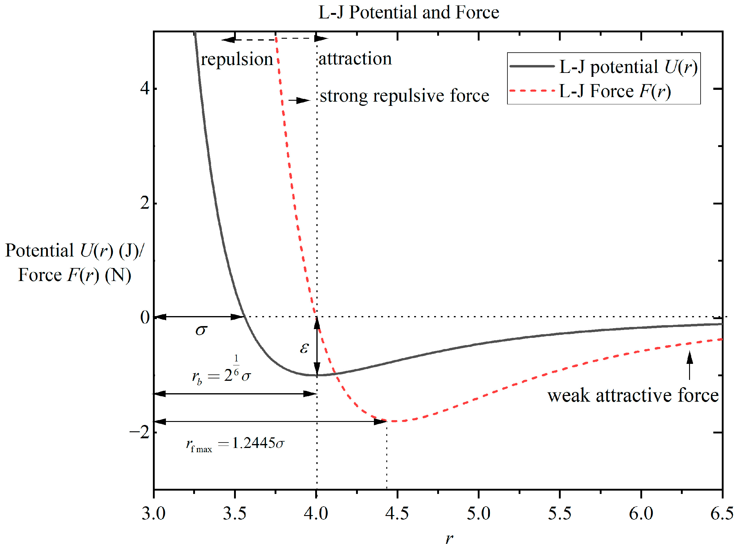
The Lennard-Jones potential, also known as the L-J potential, is primarily used in molecular dynamics to simulate simple liquids—substances where atomic interactions are solely van der Waals forces. Dependent on the pairwise distance as its only variable, the Lennard-Jones potential involves two parameters. Taking the 12-6 potential as an example, its mathematical form is given by the following:

$$U(r)=4\epsilon \left[{({\displaystyle \frac{\sigma }{r}})}^{12}-{({\displaystyle \frac{\sigma }{r}})}^6\right]$$

(1)

where $\epsilon$ represents the depth of the potential well, defined as the absolute value between the minimum of the potential energy and the zero point—this is termed the characteristic energy of the potential function. The zero point of the potential energy is located at the pairwise distance where the intermolecular potential energy is exactly zero, denoted as $r=\sigma$, which serves as the characteristic length of the potential function. Alternatively, the potential function can be expressed as follows:

$$U(r)=\epsilon \left[{({\displaystyle \frac{r_{\min }}{r}})}^{12}-2{({\displaystyle \frac{r_{\min }}{r}})}^6\right]$$

(2)

where $r_{\min }=2^{{\displaystyle \frac{1}{6}}}\sigma =1.1225\sigma$ denotes the distance between the two bodies at the bottom of the potential energy well. At this point the potential energy reaches a minimum, the repulsive force is equal to the attractive force, the force at this point is zero, and the derivative of the potential energy with respect to the position is zero; this point is also known as the equilibrium position. When the system is in equilibrium, the distance between the atoms is also roughly near the equilibrium position and its potential energy is negative. When $r<2^{{\displaystyle \frac{1}{6}}}\sigma$, two atoms behave in a mutually repulsive manner; when $r>2^{{\displaystyle \frac{1}{6}}}\sigma$, two atoms behave in a mutually attractive manner. From the point of view of physical significance, ${\displaystyle \frac{1}{r^{12}}}$ is for the two body distance closer to the mutual repulsive force of the main action term; conversely, ${\displaystyle \frac{1}{r^6}}$ is for the two body distance farther to the mutual attraction of the main action term. Figure 1 shows the 12-6 potential and its force curve.

The pairwise force corresponding to the Lennard-Jones potential is given by the following:

$$\begin{array}{ll}\hfill F(r)& =-\nabla U(r)\hfill \\ & =-{\displaystyle \frac{\mathrm{d}V(r)}{r}}r\hfill \\ & =4\epsilon (12{\displaystyle \frac{{\sigma }^{12}}{r^{13}}}-6{\displaystyle \frac{{\sigma }^6}{r^7}})r\hfill \end{array}$$

(3)

where $r_{\mathrm{eq}}=r_{\min }$ denotes the pairwise distance at the bottom of the potential well where the intermolecular force between the two bodies is zero. The following equation can also be observed:

$$r_{\mathrm{fmax}}=2{\displaystyle \frac{1}{\sqrt[6]{\frac{7}{26}}}}{r}_{\min }=1.2445\sigma$$

(4)

From the potential energy curve, it can be observed that when r is large the potential energy approaches zero and its derivative also tends to zero. This means that when two atoms are far apart, their interaction can be neglected. Therefore, in practical calculations, a truncated Lennard-Jones potential is employed. The distance at which truncation occurs is termed the cutoff radius, typically set to approximately 2.5σ. The L-J potential (n = 12) and its extended versions are all classified as pair potentials, meaning that the interaction between two atoms depends solely on that specific pair and is independent of other neighboring atoms.

2.3. Morse Potential Function

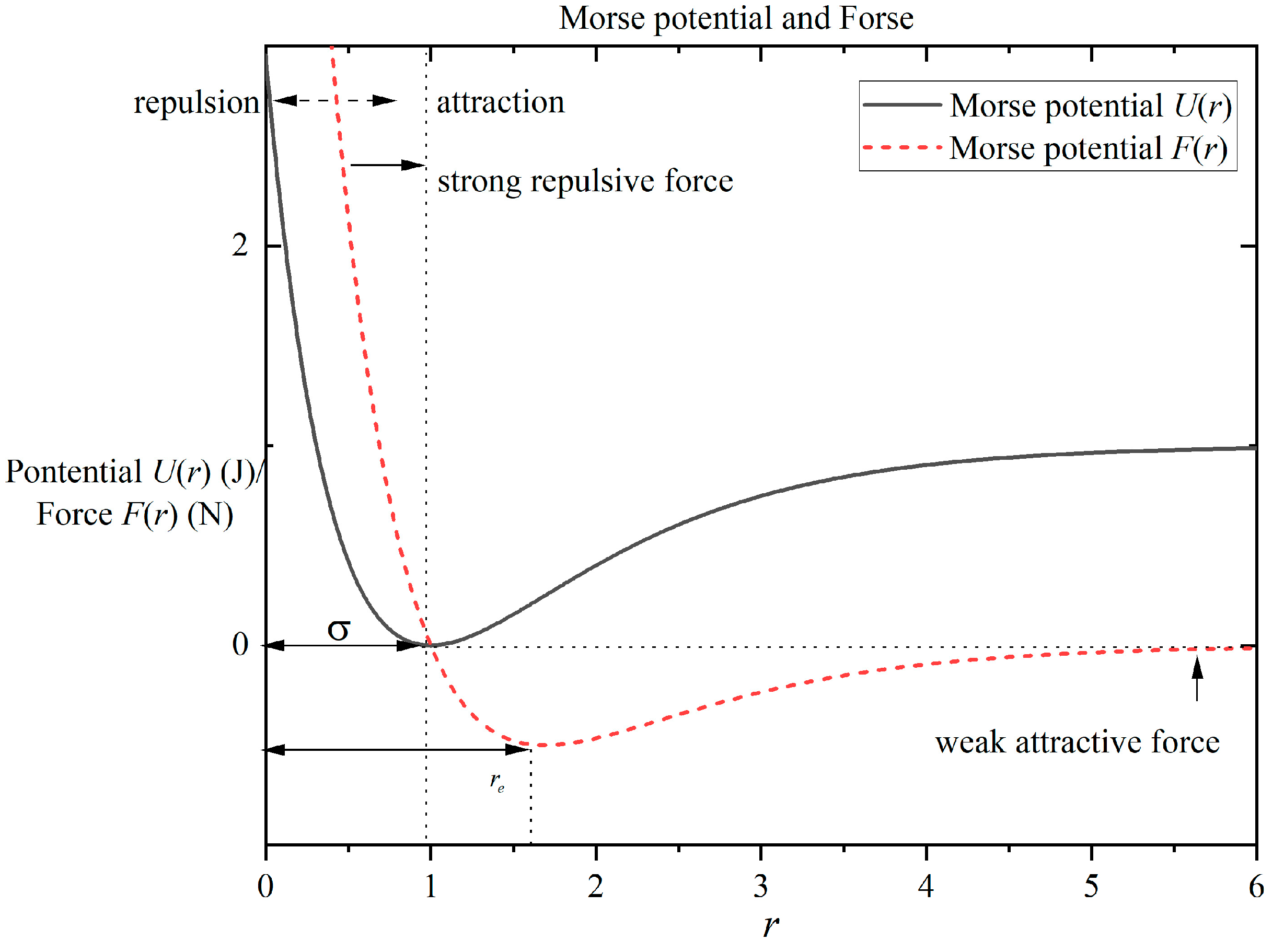
The Morse potential serves as a fundamental mathematical model in molecular dynamics, primarily designed to simulate interactions within diatomic molecules. It explicitly incorporates bond length variations between atoms, enabling an accurate description of the interplay between attractive and repulsive forces. The Morse potential effectively models the interatomic interactions as the distance between atoms changes. Its basic mathematical form is given by the basic form of the Morse potential function, which is as follows:

$$U(r)=D_e\epsilon {(1-e^{-a(r-r_e)})}^2$$

(5)

where

$\mathit{U}\left(r\right)$ is the interaction potential energy between two atoms.

$D_e$ is the dissociation energy of the molecule, i.e., the energy required to completely separate the two atoms.

$r_e$ is the equilibrium distance between atoms, defined as the interatomic distance in the molecule when the energy is at its minimum

$\alpha$ is a parameter characterizing the width of the potential energy curve, which is related to the strength of the interatomic interaction

$r$ is the distance between the two atoms.

The pairwise force corresponding to the Morse potential is given by the following:

$$\begin{array}{ll}\hfill F(r)& =-\nabla U(r)\hfill \\ & =-{\displaystyle \frac{\mathrm{d}V(r)}{r}}r\hfill \\ & =-2D_{e}a(1-e^{-a(r-r_e)})e^{-a(r-r_e)}r\hfill \end{array}$$

(6)

where $r=r_e$, $e^{-a(r-r_e)}=1$, and $F(r)=0$. This indicates that the force between the two atoms at the equilibrium position is 0, which is in accordance with the physical concept that the potential energy is minimized and force balanced at the equilibrium position. When $r>r_e$, $F(r)$ is an attractive force. Now, $e^{-a(r-r_e)}<1$, $F(r)<0$, and the atom approach the equilibrium position. When $r<r_e$, $F(r)$ is the repulsive force, and then $e^{-a(r-r_e)}>1$, so $F(r)>0$ and the atom moves away from the equilibrium position. Figure 2 shows the Morse potential and its force curve.

3. Design of UAV Swarm Dynamics Architecture Based on Molecular Dynamics

Building on the molecular dynamics principles outlined in Section 2, this section translates interatomic force models into a UAV swarm control framework. By treating each UAV as a “molecule” and using graph theory to model communication topologies, the dynamics equations and controller design are formulated to achieve velocity consensus and collective movement.

3.1. UAV Swarm Dynamics Modeling

Graph theory and matrix theory serve as the mathematical foundations for analyzing complex networks. To conduct quantitative analysis of UAV swarm behavior, modeling system dynamics through graph theory represents the most effective approach. By transforming the graph model into a matrix representation, complex networks can be systematically constructed, ultimately enabling flocking control of UAV swarms. In the UAV swarm, each UAV is treated as a node, forming a vertex set denoted as $V=\left\{v_1,v_2,v_3,\dots ,v_n\right\}$. Assuming that communication links between UAVs are bidirectional, these links are abstracted as edges defined by the set E. If there is a connection between nodes i and j, then $\left\{v_i,v_j\right\}\in E\subset {\left[V\right]}^2$. Consequently, the UAV swarm is abstracted as an undirected, acyclic simple graph $G=\left\{V,E,W\right\}$, where W is the edge weight matrix. The base station issues commands to the leader UAV, specifying its position and velocity, which is used to guide the entire swarm to fly toward a predetermined target.

For each UAV, consider its dynamics equations, which typically include state variables such as position, velocity, and acceleration. Without loss of generality, UAVs are abstracted as point masses moving in three-dimensional space, neglecting their shape, dynamic characteristics, and other physical details. Assume all UAVs have a unit mass (i.e., mass = 1), thus simplifying the expressions for their kinetic and potential energies. Suppose N UAVs move in an n-dimensional Euclidean space, then the kinematic equations for these point masses are given by the following:

$$\begin{array}{cc}\left\{\begin{array}{c}{\dot{p}}_i=v_i\\ {\dot{v}}_i=u_i\end{array}\right.& i=1,\dots ,n\end{array}$$

(7)

where $p_i,v_i$ and u_i denote the position vector, velocity vector, and acceleration vector of UAV i, respectively.

The undirected graph $V(t)$ constructed for the UAV swarm at time t is composed of vertices and edges, where the vertex set is denoted by $V=\left\{1,2,\dots ,n\right\}$ and the edge set by $E(t)=\left\{(i,j)\in V\times V,j\in {𝒩}_i(t)\right\}$. It is assumed that the equilibrium distance of the UAV swarm is $r_b$ and the sensing radius is r. In this case, the neighborhood of a UAV is defined as follows:

$${𝒩}_i(t)=\left\{j|‖q_i-q_j‖<r,j\in V,j\ne i\right\}$$

(8)

By employing the Laplacian matrix to model the UAV swarm network, the matrix L is defined as follows:

$$L(t)={\left[L_{ij}\right]}_{m\times n}$$

(9)

where $L_{ij}={\displaystyle \sum _{j=1,i\ne j}^m{a}_{ij}}$ and $L_{ij}=-a_{ij}$. In the function, only if $j\in {𝒩}_i$ then $a_{ij}=1$, otherwise $a_{ij}=0$. The function satisfies the following sum-of-squares property:

$$z^T(L\otimes I_m)z={\displaystyle \frac{1}{2}}{{\displaystyle \sum _{,j\in {,}_i}{a}_{ij}j(z_i-z_j)}}^2$$

(10)

To avoid collisions among UAVs, the expected evolution objective of the UAV swarm is specified as follows:

$${‖q_i-q_j‖}_2=d,(i,j)\in E,d<r$$

(11)

3.2. UAV Swarm Controller Design

Assume that the control input at time t is as follows:

$$u_i(t)=f_i^{\alpha }(t)+f_i^{\beta }(t)+h_i(t)f_i^{\gamma }(t)$$

(12)

where $f_i^{\alpha }(t)$ represents the gradient term of the potential function, which is employed to realize separation and aggregation in the Boid model. The physical meaning of the potential function gradient term is the force exerted by the potential function, with its specific mathematical expression given as follows:

$$f_i^{\alpha }(t)={\displaystyle \sum _{j\in N_i}{f}_{ij}^{L-J}(t)}$$

(13)

where $f_{ij}^{L-J}(\ge t)$ represents the force exerted by the potential function between the i-th agent and the j-th agent. The corresponding force in the Lennard-Jones potential is shown in (3), and the force of the Morse potential is shown in (6).

$f_i^{\beta }(t)$ is the velocity consensus term, which is used to achieve velocity matching among UAVs. Its expression is as follows:

$$f_i^{\beta }(t)={\displaystyle \sum _{j\in N_i}{a}_{ij}(t)(p_i-p_j)}$$

(14)

where $a_{ij}$ is elements of the Laplacian matrix. Then, $a_{ij}=1$ if and only if $j\in {𝒩}_i$, and $a_{ij}=0$ otherwise.

$h_i(t)f_i^{\gamma }(t)$ is pinning control term. $f_i^{\gamma }(t)$ denotes the information received from the virtual leader, with its mathematical expression given by the following:

$$f_i^{\gamma }(t)=c_1^{\gamma }\left(q_{\gamma }(t)-q_i(t)\right)+c_2^{\gamma }\left(p_{\gamma }(t)-p_i(t)\right)$$

(15)

where $p_{\gamma }\in {\mathrm{R}}^n$ is the velocity vector of the virtual leader at time t, and $c_1^{\gamma }$ and $c_2^{\gamma }$ are positive coefficients. $h_i(t)$ is a parameter related to the selection of pinning nodes, which corresponds to determining pinning nodes; its mathematical expression at time t is given by the following:

$$h_i(t)=\left\{\begin{array}{cc}1,\hfill & i\mathrm{is}\mathrm{pinning}\mathrm{node}\\ 0,\hfill & i\mathrm{is}\mathrm{NOT}\mathrm{pinning}\mathrm{node}\end{array}\right.$$

(16)

$$H=\mathrm{diag}(h_1,h_2,\dots ,h_N)$$

(17)

N is the number of agents. Its augmented Laplace matrix is defined as follows:

$$A=L+kH$$

(18)

The set of all agent nodes is denoted by V. Let $V_b\subset V$ be a non-empty subset of V. $V_b$ is referred to as the set of pinning nodes, and the remaining nodes are followers.

4. Theorems and Proofs

This section focuses on proving the stability of UAV swarm systems using Liapunov’s second method. The proof of truncated potential is shown in Appendix B.

Assumption 1.

The initial state of the undirected graph $\mathrm{G}(0)$ is fully connected.

Assumption 2.

No initial collision.

Assumption 3.

Virtual leader speed fixed.

Theorem 1.

Assume that the equations of motion of a UAV swarm are shown in (7) and the input control is shown in (11). Then, any one of the drafting nodes is selected:

(1)

The relative positions of all intelligences will eventually converge to lattices; 

(2)

All the speed of UAVs will converge to that of the virtual leader $p_{\gamma }(t);$

(3)

UAVs do not collide with each other; 

(4)

The tie node position will converge to the virtual leader $q_{\gamma }(t)$ position. 

Proof of Theorem 1.

Assume that the tracking error of the agent with the virtual leader is as follows:

$${\tilde{q}}_i(t)=q_i(t)-q_{\gamma }(t),{\tilde{p}}_i(t)=p_i(t)-p_{\gamma }(t).$$

(19)

The distance between the intelligences is as follows:

$$q_{ij}(t)=q_i(t)-q_j(t).$$

(20)

The total energy function of multi-agents is defined as shown in Equation (21) and consists of total potential energy and total kinetic energy:

$$Q(t)={\displaystyle \frac{1}{2}}{\displaystyle \sum _{i=1}^m\left({\psi }_i(t)+{\tilde{p}}_i{(t)}^T{\tilde{p}}_i(t)\right)}$$

(21)

Design its potential energy function as follows:

$${\psi }_i({\tilde{q}}_i)={\displaystyle \frac{1}{2}}{\displaystyle \sum _{i=1}^m{U}_i({\tilde{q}}_i)+h_i(t){\tilde{q}}_i^T{\tilde{q}}_i}$$

(22)

The energy equation can be rewritten as follows:

$$Q\left(t\right)={\displaystyle \frac{1}{2}}{\displaystyle \sum _{i=1}^n\left({\psi }_i\left(t\right)+{\tilde{p}}_i{\left(t\right)}^T{\tilde{p}}_i\left(t\right)\right)}$$

(23)

Taking the derivative with respect to time t gives the following:

$$\begin{array}{cc}\hfill \dot{Q}\left(t\right)=& -c_2^{\alpha }\tilde{p}{\left(t\right)}^T\left(L\left(t\right)\otimes I_m\right)\tilde{p}\left(t\right)\hfill \\ & -c_2^{\gamma }{\displaystyle \sum _{i=1}^m{h}_i\left(t\right){\tilde{p}}_i{\left(t\right)}^T{\tilde{p}}_i\left(t\right)}\hfill \\ & =-\tilde{p}{\left(t\right)}^T\left(\left(c_2^{\alpha }L\left(t\right)+c_2^{\gamma }H\left(t\right)\right)\otimes I_m\right)\tilde{p}\left(t\right)\hfill \\ & \le 0\hfill \end{array}$$

(24)

where L is the Laplace matrix corresponding to the UAV network, $H=diag[h_1\dots h_n]$. Both matrices L and H are semi-positive definite matrices, and it is easy to know that $\left(\left(c_2^{\alpha }L\left(t\right)+c_2^{\gamma }H\left(t\right)\right)\otimes I_m\right)$ is a semi-positive definite array. At the moment t, $\dot{Q}\le 0$, which means that $Q\left(t\right)$ is a non-increasing matrix and that the total energy of the system continues to decay. This indicates that all agents are gradually adjusting their positions in order to ensure that they keep the desired distance from the surrounding intelligences and adjust their speeds to be consistent with the virtual leader. Theorem 1(2) is proved.

From the definition of the potential energy function $U(q)$, ${\displaystyle \sum _{i=1}^N{U}_i(\left|\right|r{\left|\right|}_{\alpha })\le Q(0)\le }{Q}_{\max }$, and the distance between two nodes that are neighbors of each other at time t should be less than r, which means the edges that already exist in the network will not be broken. Assuming that m new edges are added to the network after time has elapsed, then the following is obtained:

$$Q(t+\Delta t)=Q_0+mU(||r-\epsilon |{|}_{\alpha })\le Q_{\max }.$$

(25)

This demonstrates that as time evolves, no existing edges within the system will be disconnected. Given that the initial network G(0) is connected, the system will remain globally connected at all times. Theorem 1(1) is proved.

Without loss of generality, assume that at any arbitrary time, $\left[t_0,t_1\right]$, if a collision occurs between two UAVs $i$ and $j$ at $t_s\in \left[t_0,t_1\right]$ then ${\Phi }_i\left(t\right)$ will increase, leading to an overall increase in the total energy, $Q(t)$, of the system. This directly contradicts with $\dot{Q}(t)⩽0$ that the total energy remains non-increasing over time. By extending this logic to all time instants, the UAV swarm is guaranteed to avoid collisions entirely at $\left[t_k,t_{k+1}\right]$, thus completing the proof of Theorem 1(3).

All agents move with the virtual leader at the same velocity. During the motion, all agents gradually adjust to maintain the desired distance from neighboring agents, i.e.,

$${\dot{p}}_1={\dot{p}}_2=\dots ={\dot{p}}_n={\dot{p}}_0=0$$

(26)

When $p_i(t)=p_{\gamma }(t)$ and when i is not a pinning node, as can be seen from (12) to (15), then the following is obtained:

$$u_i(t)={\displaystyle \sum _{j\in N_i}{f}_{ij}^{L-J}(t)}=0$$

(27)

When node i is a pinning node, it follows that:

$$u_i(t)={\displaystyle \sum _{j\in N_i}{f}_{ij}^{L-J}(t)}-c_1^{\gamma }\left(q_{\gamma }(t)-q_i(t)\right)$$

(28)

It follows from the symmetry of the potential energy that:

$${\displaystyle \sum _{j\in N_i}{f}_{ij}^{L-J}(t)}=0$$

(29)

$$q_i(t)=q_{\gamma }(t)$$

(30)

Assuming there are multiple pinning nodes, without loss of generality, suppose there are two pinning nodes i,j, from which the following can be obtained:

$$q_i(t)=q_j(t)=q_{\gamma }(t)$$

(31)

It follows from Theorem 1(3) that no collisions will occur between UAVs, i.e.,

$$q_i(t)\ne q_j(t)$$

(32)

A contradiction arises from (31) and (32), implying that the entire UAV swarm will eventually converge to a unified network. Meanwhile, according to (30), the positions of pinning nodes tend to converge to that of the virtual leader. Thus, the proof is completed. □

5. Simulation Experiment

To validate the proposed molecular dynamics-based control strategy, this section presents a series of simulation experiments. The impact of different potential functions and swarm sizes on consensus performance is systematically evaluated, along with three-dimensional applicability tests. Experimental results demonstrate the effectiveness of the Morse potential in accelerating convergence and ensuring collision-free swarming behavior.

5.1. Experimental Design and Parameter Selection

A two-degree-of-freedom dynamic model of quadrotor UAVs was developed, incorporating actuator constraints to mimic the following real-world flight scenarios: a ±270° heading angle limitation and a linear velocity threshold of 0.3 m/s. The UAV swarm was configured with a fully connected communication topology and an inter-agent equilibrium distance of 1 m. The framework was constructed using the truncated potential function, and its truncation distance is 2 m. $D_e$ of Morse potential is set as 1 and ε of L-J potential is set as 1. To guarantee the reliability of experimental outcomes, each test was replicated 10 times, and the average convergence time was adopted as the final result. In this study, theoretical mathematical simulations were conducted to validate the proposed algorithm under idealized conditions. The system dynamics were modeled using (12)–(16). The simulation experiment was verified using Matlab 2019a, and the PC is Acer N22C1.

This research presents a comprehensive validation framework for UAV swarm consensus control, systematically evaluating the effects of potential functions and system parameters on convergence performance. In fixed-scale scenarios (n = 40 agents), the empirical comparisons that were conducted include Lennard-Jones potentials with varying exponents, Morse potentials with parametric variations, the baseline Vicsek model, and a Gaussian kernel-enhanced Vicsek variant [28]. Standardized metrics were established to quantify consensus time and accuracy across models. Building upon baseline validations, the parameter space was expanded to investigate swarm size effects. A multi-level consensus evaluation system was constructed to investigate the time costs required for UAV swarms of different scales to achieve varying consensus levels and analyze the influence law of swarm size on time performance. Finally, 3D simulations verified the method’s scalability to three-dimensional operational environments.

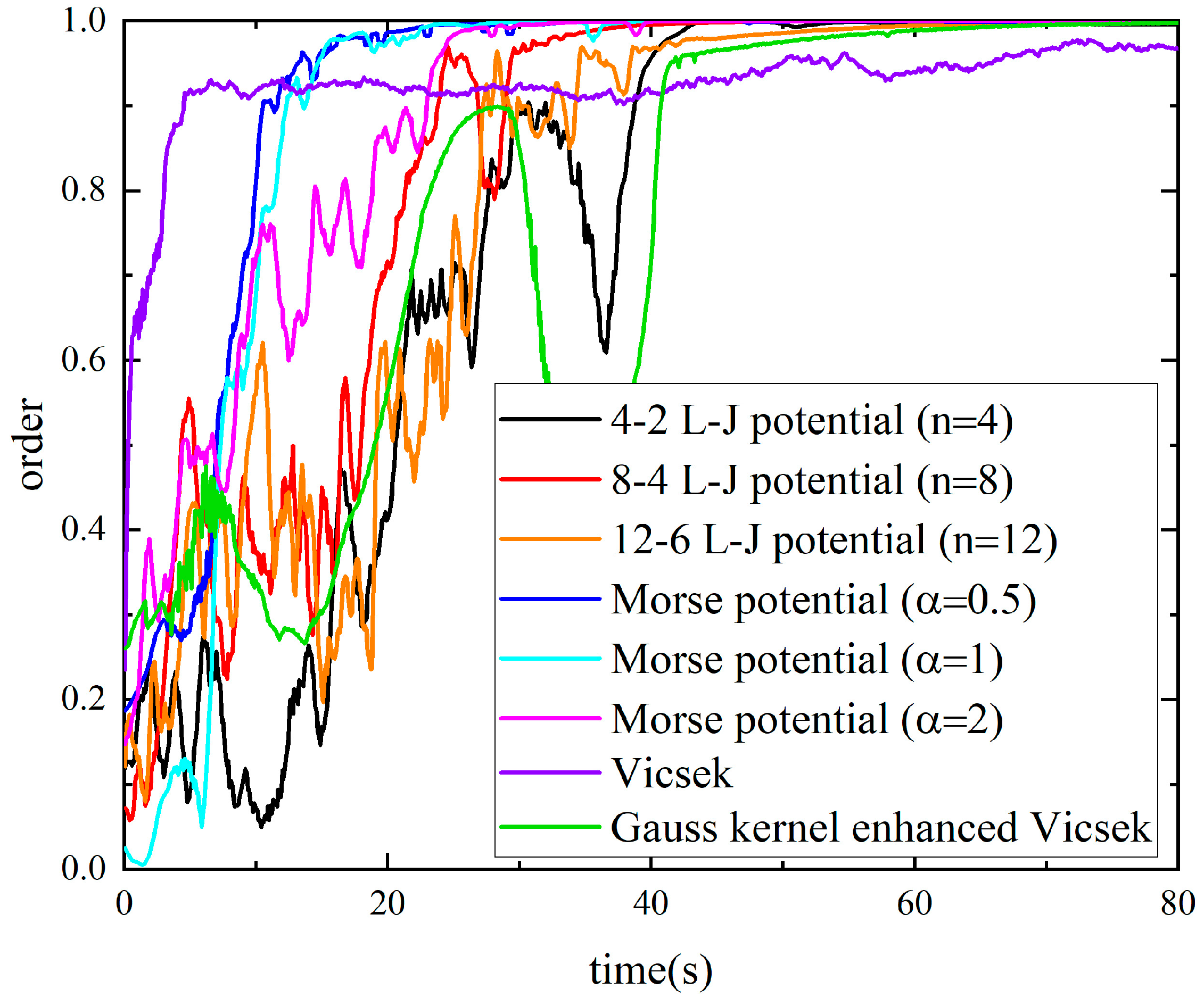
5.2. Experiment 1: Effect of Different Potential Functions

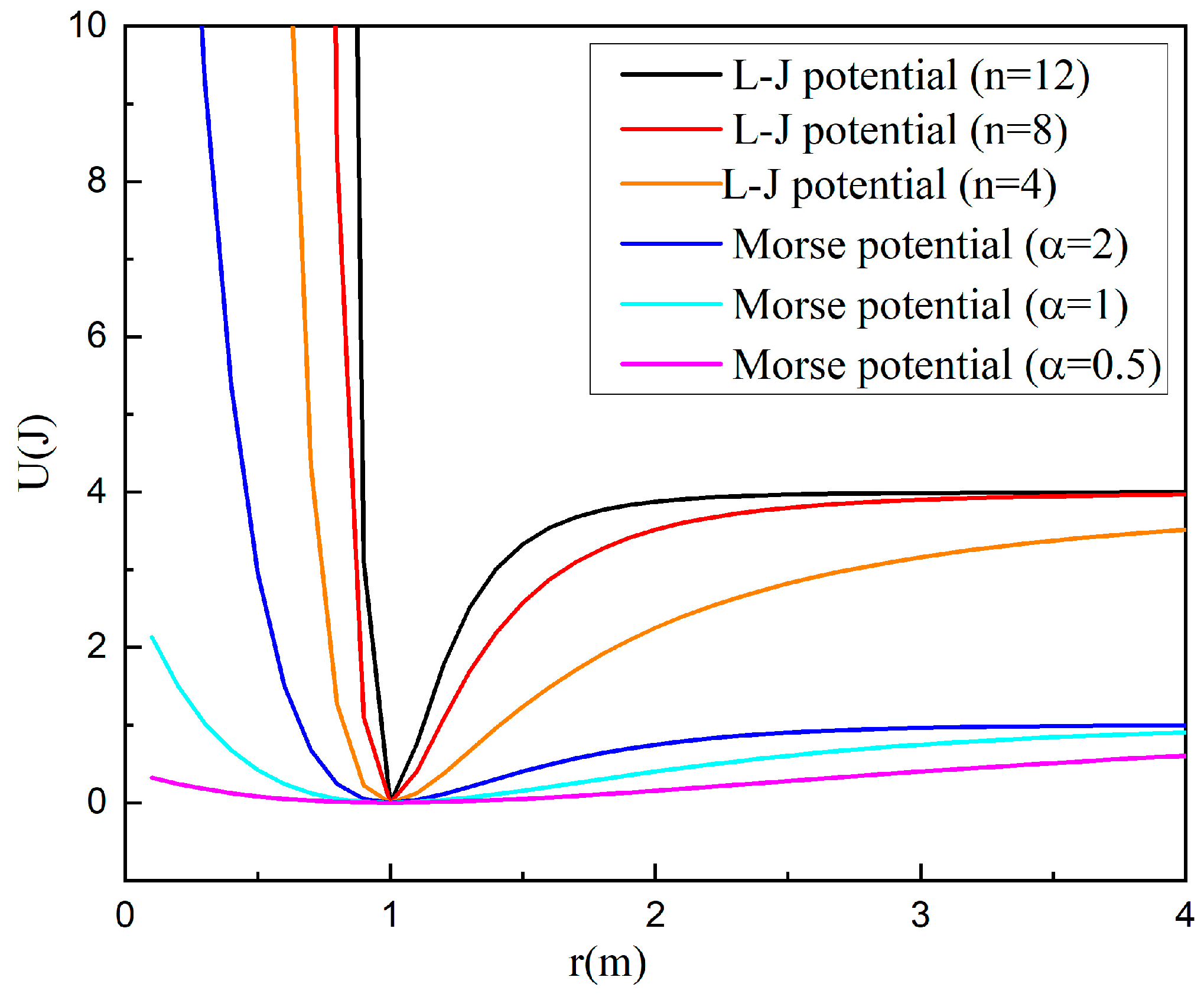
The number of the UAV swarm is fixed at 40 to verify the effect of different potential functions on the consistency of the swarm. Different powers of the Lennard-Jones potential function (n = 4, 8, and 12) and α of Morse potential function (α = 0.5, 1, and 2) are chosen, respectively. The different potential function curves are shown in Figure 3. For example, in the Morse potential function the value of α affects the steepness of the potential energy curve and thus influences the rate of change in the interaction force between UAVs with distance. 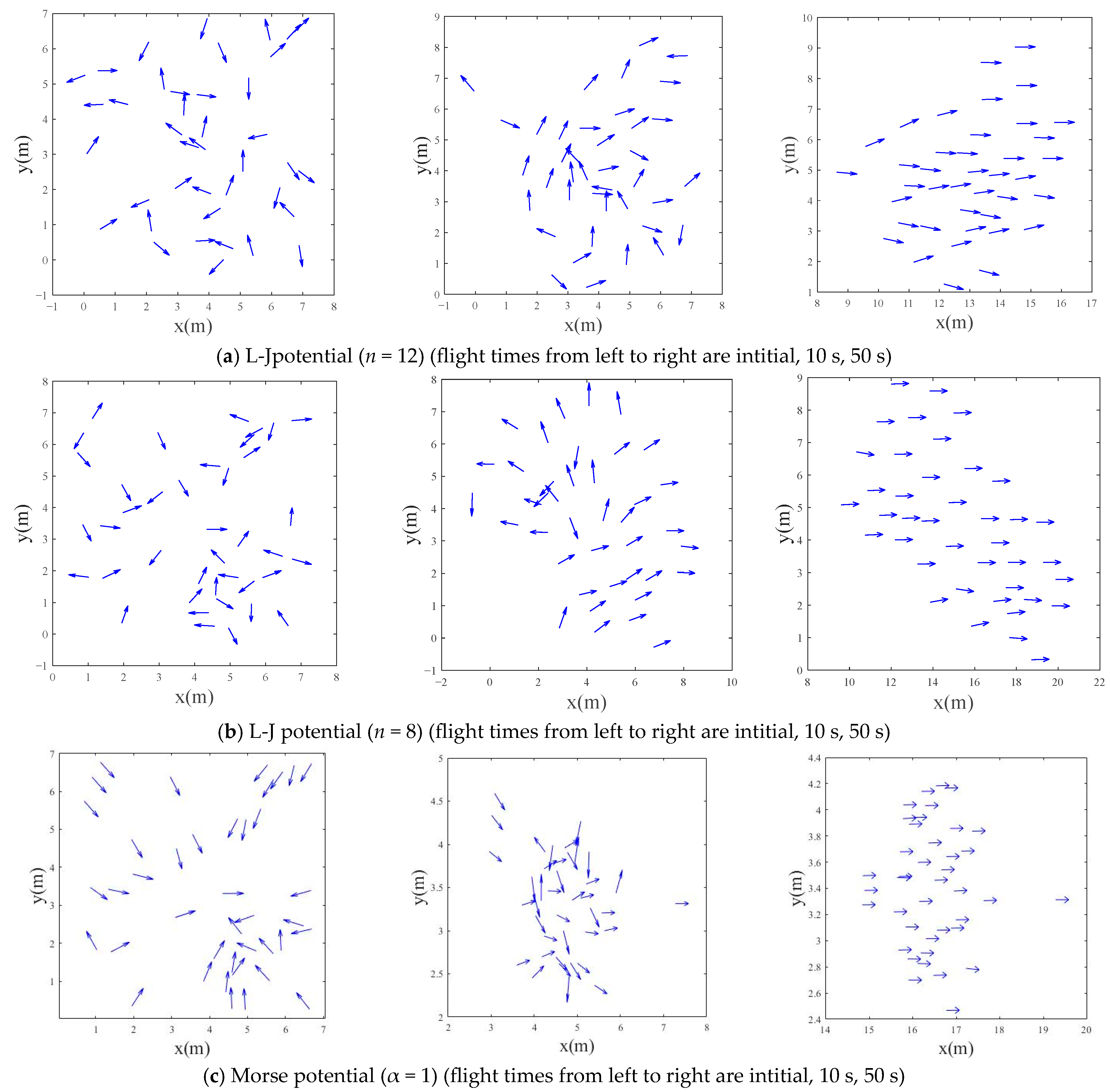A smaller value of α makes the changes in the attractive and repulsive forces relatively gentle, which is beneficial for the UAV swarm to maintain a stable relative position relationship within a large range and also shows a faster speed of achieving consistency and smaller fluctuations in the experiment. The states at different moments are shown in Figure 4. The arrow direction is the direction of UAV speed: Figure 5 shows the flight trajectory of the UAV swarm and Figure 6 shows the variation curve of the sequence parameters.

Table 1. Time required to reach consistency for potential functions of different powers.

Order Parameter\ Potential Function	Vicsek	Gauss Kernel Enhanced Vivcsek [28]	L-J Potential			Morse Potential
			n = 4	n = 8	n = 12	α = 0.5	α = 1	α = 2
0.9	21.6 ± 18.2 s	34.5 ± 1.9 s	33.0 ± 2.7 s	30.0 ± 1.2 s	38.3 ± 2.0 s	26.6 ± 0.4 s	30.0 ± 1.2 s	35.4 ± 2.4 s
0.95	-	37.3 ± 1.8 s	37.0 ± 2.9 s	37.5 ± 2.4 s	45.3 ± 3.0 s	30.8 ± 0.7 s	35.8 ± 1.7 s	38.9 ± 2.3 s
0.995	-	54.3 ± 3.5 s	55.4 ± 2.9 s	61.6 ± 6.2 s	69.9 ± 6.6 s	49.0 ± 3.0 s	56.1 ± 3.2 s	56.5 ± 3.7 s

shows the time required for the UAV swarm to reach consistency.

To verify the repeatability of the method, 10 sets of UAV swarms with different initial states were used as verification. Through experimental verification, it can be known that the standard Vicsek method exhibits relatively poor repeatability. The reason is that each particle adds a random angle (such as Gaussian white noise) when updating its direction, leading to possible differences in the specific trajectories of each simulation even with completely identical initial conditions, thus causing larger fluctuations. Additionally, it cannot achieve a higher level of consensus. The UAV swarm control method based on molecular dynamics requires approximately 30 s to achieve consensus, among which the result of the Morse potential function is slightly better than that of the L-J potential function. The reason lies in the difference in the strength of their attractive forces. Additionally, the Vicsek model and its Gaussian kernel-enhanced variant rely on random noise for direction updates, omit explicit repulsive force modeling, and lack collision avoidance terms, rendering them susceptible to collisions. In contrast, our molecular dynamics-based approach generates substantial repulsive forces when UAVs approach close proximity, attributable to the inclusion of a repulsive term, thereby eliminating collision occurrences. However, since both the Lennard-Jones potential and Morse potential are pair-wise potential functions they neglect multi-agent interactions, consequently leading to ineffective system convergence to equilibrium distance.

As shown in Figure 3, the attractive and repulsive forces of the Morse potential with α = 0.5 change relatively smoothly with distance and so the generated fluctuations are relatively small, allowing faster consensus achievement with relatively stable time. For each potential function, as the attractive and repulsive forces increase, the time required to achieve consensus gradually increases and the uncertainty also continuously increases.

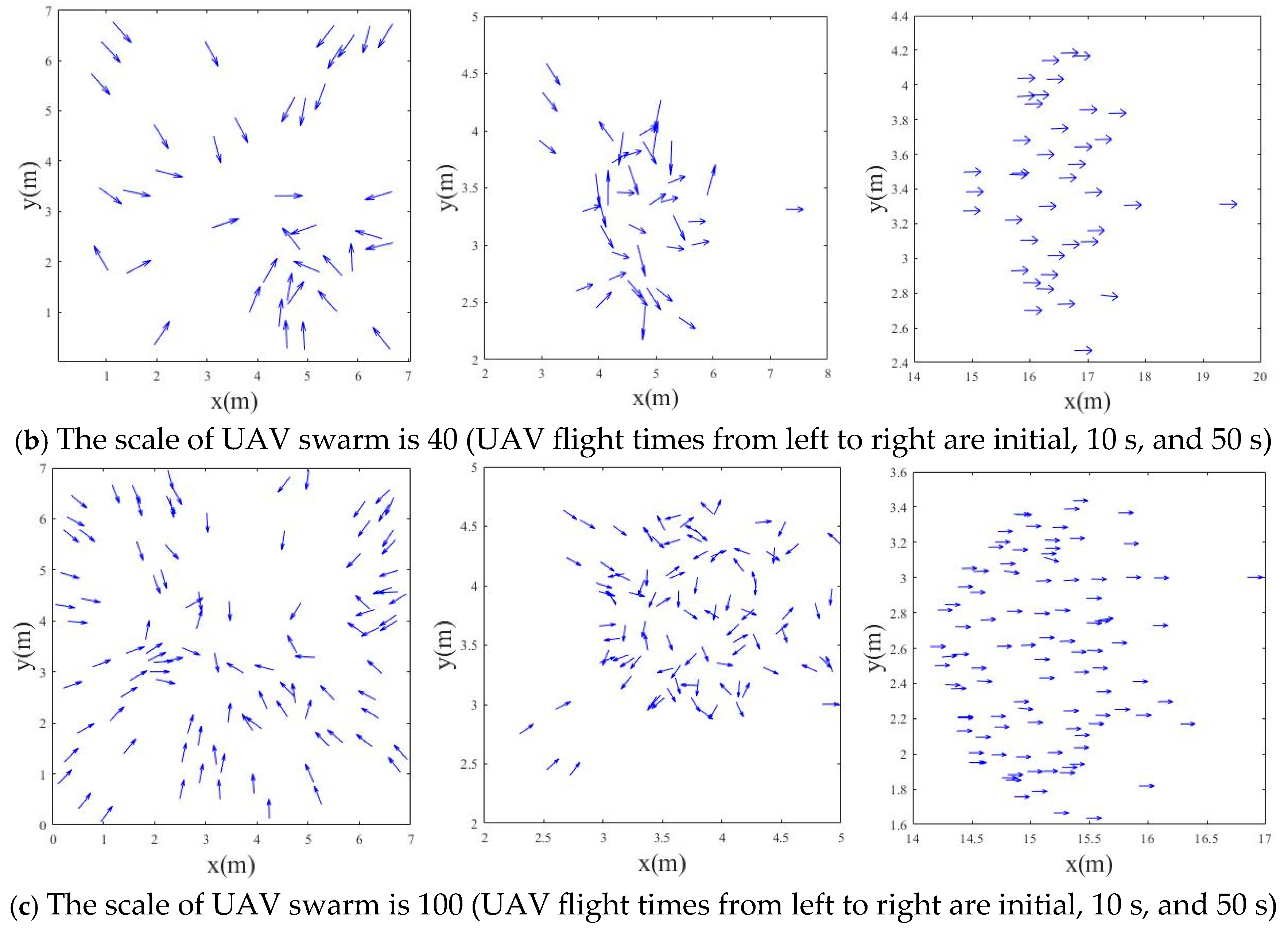
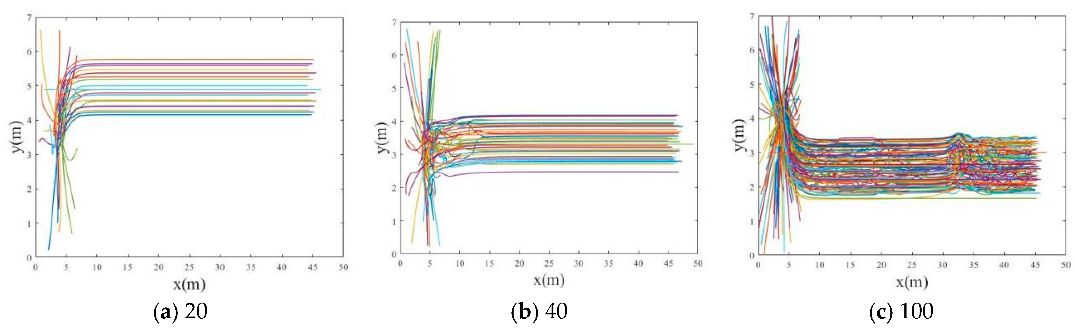
5.3. Experiment 2: Impact of Swarm Size

The UAV swarm sizes are set to 20, 40, and 100, and the rest of the parameters are consistent with Experiment 1. We then verify the effect of different swarm sizes on the consistency of UAVs. The time of Morse potential (α = 0.5) to reach consistency in different sizes of UAV swarm is shown in

Table 2. Time required to reach consistency for different powers of the potential function.

Order Parameter\Swarm Size	20		40		100
Potential	L-J	Morse	L-J	Morse	L-J	Morse
0.9	30.4 ± 2.4 s	24.2 ± 1.0 s	38.3 ± 2.0 s	26.6 ± 0.4 s	41.3 ± 2.3 s	29.7 ± 0.8 s
0.95	34.3 ± 2.0 s	27.2 ± 1.1 s	45.3 ± 3.0 s	30.8 ± 0.7 s	44.6 ± 2.5 s	32.8 ± 1.1 s
0.995	55.4 ± 2.7 s	43.7 ± 2.2 s	69.9 ± 6.6 s	49.0 ± 3.0 s	66.8 ± 6.1 s	48.5 ± 2.5 s

. Figure 7 shows the working state of the UAV swarm of different sizes at different moments under the Morse potential (α = 0.5). Figure 8 shows the flight trajectories of the UAV swarm of different sizes. The UAV swarm size is directly proportional to the convergence speed of UAVs, but there is a problem of large dependence on the initial value. Figure 9 shows the variation curves of the ordinal coefficients of the L-J potential and Morse potential function at different UAV scales. During the simulation, it was found that although the Morse and L-J potential functions effectively avoid collisions under normal conditions, they fail to converge to the equilibrium distance in extreme scenarios (such as dense swarm conditions). Moreover, as the swarm scale increases, the UAV density increases, causing the equilibrium distance to be smaller than the preset value.

Both of the two methods can effectively achieve consistency control. By introducing the Morse potential function to construct the system model, the convergence process can be significantly accelerated. In the application scenarios of UAV swarms of different scales, the convergence speed is increased by an average of 26% compared with the situation without using this function, which greatly optimizes the efficiency of the swarm in tasks such as achieving consistency.

5.4. Experiment 3: Consistency Verification Test in Three-Dimensional Space

A swarm of 40 unmanned aerial vehicles (UAVs) was employed to verify the consistency of collective behavior in three-dimensional space. A total of 10 sets of UAV swarms with different initial states were used as verification. To model real-world conditions, a three-dimensional analytical dynamics framework was constructed using the truncated Morse potential function, and its truncation distance was set to 2 m. An inertia coefficient of 0.8 was specified to ensure the swarm adheres to inertial flight dynamics. Figure 10 illustrates the swarm’s configurations at discrete time instances, where arrow orientations denote the velocity directions of individual UAVs. Figure 11 presents the trajectory profiles of the UAV swarm, visualizing its spatiotemporal movement patterns in the three-dimensional domain. Experimental validation confirms that the proposed method effectively achieves consistency control in three-dimensional space. Figure 12 shows the variation curve of the sequence parameters in three-dimensional space. When the order parameter of the UAV swarm reaches 95%, its consensus time is 8.8 ± 1.4 s, demonstrating its effective achievement of consensus. The UAV swarm achieves consensus faster than in two-dimensional experiments, which is attributed to the introduction of an inertial coefficient. This inertial coefficient reduces the fluctuations in directional changes in each UAV, thereby enabling faster attainment of directional consensus.

6. Conclusions

This study presents a molecular dynamics-based consistency control framework for UAV swarms, addressing the challenge of achieving efficient and stable collective behavior in complex scenarios. This method has important application significance for the requirements of different mission scenarios of UAV swarms, such as wide-area reconnaissance, hovering, and aggregation and diffusion of the swarm. Drawing inspiration from interatomic interactions, each UAV is modeled as a “molecule”, with inter-UAV forces described by potential functions that emulate the balance between attractive (cohesion-maintaining) and repulsive (collision-avoiding) forces—principles rooted in natural particle dynamics. This approach leverages scalable, low-complexity potential functions, specifically the Lennard-Jones and Morse potentials, to construct a Vicsek-based dynamic model for swarm interactions. Lyapunov stability analysis confirms that the system converges to a consistent state. The framework facilitates the emergence of self-organized swarming, enhancing both collaborative efficiency and robustness. Experimental results demonstrate the superior performance of the Morse potential in consistency control as a 40-UAV swarm achieves 90% consistency in 26.6 ± 0.4 s under α = 0.5, outperforming the best Lennard-Jones configuration by 26%. This superiority is attributed to the Morse potential’s smoother force–distance profile, which balances responsiveness and stability across varying swarm scales.

In the future, we will conduct further research specifically on aspects such as scalability and computational complexity. We will discuss strategies to adapt our methods to larger-scale systems. Furthermore, we plan to use many-body potential functions such as the Tersoff potential and the EAM potential to address the issue of the convergence distance and further optimize the process to reduce its time complexity. Finally, we will refine the model in the three-dimensional space to make it more consistent with real-world scenarios.

References

1. Han, F.; Liu, J.; Li, J.; Song, J.; Wang, M.; Zhang, Y. Consensus control for multi-rate multi-agent systems with fading measurements: The dynamic event-triggered case. Syst. Sci. Control Eng. 2023, 11, 2158959. [Google Scholar] [CrossRef]
2. Andrade, S.; Pires, A.; Almeida, P.; Coutinho, I.; Bayse, S.; Oliveira, P. Population Structure and Reproductive Biology of Lane Snapper, Lutjanus synagris (Lutjanidae) Caught in the Reef Fish Fishery of Pernambuco, Brazil. J. Ichthyol. 2024, 64, 1060–1073. [Google Scholar] [CrossRef]
3. Okubo, A. Dynamical aspects of animal grouping: Swarms, schools, flocks, and herds. Adv. Biophys. 1986, 22, 1–94. [Google Scholar] [CrossRef]
4. Parrish, J.K.; Viscido, S.V.; Grünbaum, D. Self-organized fish schools: An examination of emergent properties. Biol. Bull. 2002, 202, 296–305. [Google Scholar] [CrossRef]
5. Potts, W.K. The chorus-line hypothesis of manoeuvre coordination in avian flocks. Nature 1984, 309, 344–345. [Google Scholar] [CrossRef]
6. Zavlanos, M.M.; Tanner, H.G.; Jadbabaie, A.; Pappas, G.J. Hybrid Control for Connectivity Preserving Flocking. IEEE Trans. Autom. Control 2009, 54, 2869–2875. [Google Scholar] [CrossRef]
7. Zhang, H.T.; Zhai, C.; Chen, Z. A General Alignment Repulsion Algorithm for Flocking of Multi-Agent Systems. IEEE Trans. Autom. Control 2011, 56, 430–435. [Google Scholar] [CrossRef]
8. Bhamu, N.; Verma, H.; Dixit, A.; Bollard, B.; Sarangi, S.R. SmrtSwarm: A Novel Swarming Model for Real-World Environments. Drones 2023, 7, 573. [Google Scholar] [CrossRef]
9. Wang, F.; Huang, J.; Low, K.H.; Hu, T. Collective Navigation of Aerial Vehicle Swarms: A Flocking Inspired Approach. IEEE Trans. Intell. Veh. 2024, 9, 1040–1053. [Google Scholar] [CrossRef]
10. Nilsson, C.; Bäckman, J.; Dokter, A.M. Flocking behaviour in the twilight ascents of Common Swifts Apus apus. Ibis 2019, 161, 674–678. [Google Scholar] [CrossRef]
11. Reynolds, C.W. Flocks, herds and schools: A distributed behavioral model. SIGGRAPH Comput. Graph. 1987, 21, 25–34. [Google Scholar] [CrossRef]
12. Vicsek, T.; Czirók, A.; Ben-Jacob, E.; Cohen, I.I.; Shochet, O. Novel type of phase transition in a system of self-driven particles. Phys. Rev. Lett. 1995, 75, 1226–1229. [Google Scholar] [CrossRef] [PubMed]
13. Olfati-Saber, R.; Murray, R.M. Consensus problems in networks of agents with switching topology and time-delays. IEEE Trans. Autom. Control 2004, 49, 1520–1533. [Google Scholar] [CrossRef]
14. Gudeta, S.G.; Karimoddini, A.; Davoodi, M.R.; Raptis, I.A. Leaderless Swarm Formation Control: From Global Specifications to Local Control Laws. In Proceedings of the 2021 American Control Conference (ACC), New Orleans, LA, USA, 25–28 May 2021; pp. 808–813. [Google Scholar]
15. Phadke, A.; Medrano, F.A.; Sekharan, C.N.; Chu, T. Designing UAV Swarm Experiments: A Simulator Selection and Experiment Design Process. Sensors 2023, 23, 7359. [Google Scholar] [CrossRef]
16. Wang, T.; Zhao, S.; Xia, Y.; Pan, Z.; Tian, H. Consensus Control of Large-Scale UAV Swarm Based on Multi-Layer Graph. Drones 2022, 6, 402. [Google Scholar] [CrossRef]
17. Guo, C.; Zhu, P.; Zhou, Z.; Lang, L.; Zeng, Z.; Lu, H. Imitation Learning with Graph Neural Networks for Improving Swarm Robustness under Restricted Communications. Appl. Sci. 2021, 11, 9055. [Google Scholar] [CrossRef]
18. Han, W.; Wang, J.; Wang, Y.; Xu, B. Multi-UAV Flocking Control With a Hierarchical Collective Behavior Pattern Inspired by Sheep. IEEE Trans. Aerosp. Electron. Syst. 2024, 60, 2267–2276. [Google Scholar] [CrossRef]
19. Zhou, X.; Wen, X.; Wang, Z.; Gao, Y.; Li, H.; Wang, Q.; Yang, T.; Lu, H.; Cao, Y.; Xu, C.; et al. Swarm of micro flying robots in the wild. Sci. Robot. 2022, 7, eabm5954. [Google Scholar] [CrossRef]
20. Bai, C.; Yan, P.; Piao, H.; Pan, W.; Guo, J. Learning-Based Multi-UAV Flocking Control With Limited Visual Field and Instinctive Repulsion. IEEE Trans. Cybern. 2024, 54, 462–475. [Google Scholar] [CrossRef]
21. Wei, Z.; Wei, R. UAV Swarm Rounding Strategy Based on Deep Reinforcement Learning Goal Consistency with Multi-Head Soft Attention Algorithm. Drones 2024, 8, 731. [Google Scholar] [CrossRef]
22. Ma, C.; Li, A.; Du, Y.; Dong, H.; Yang, Y. Efficient and scalable reinforcement learning for large-scale network control. Nat. Mach. Intell. 2024, 6, 1006–1020. [Google Scholar] [CrossRef]
23. Xu, H.; Zhang, Y.; Zhou, B.; Wang, L.; Yao, X.; Meng, G.; Shen, S. Omni-Swarm: A Decentralized Omnidirectional Visual–Inertial–UWB State Estimation System for Aerial Swarms. IEEE Trans. Robot. 2021, 38, 3374–3394. [Google Scholar] [CrossRef]
24. Bu, Y.; Yan, Y.; Yang, Y. Advancement Challenges in UAV Swarm Formation Control: A Comprehensive Review. Drones 2024, 8, 320. [Google Scholar] [CrossRef]
25. Liu, L.; Jiao, Y.; Yang, M.; Wu, L.; Long, G.; Hu, W. Network Pharmacology, Molecular Docking and Molecular Dynamics to Explore the Potential Immunomodulatory Mechanisms of Deer Antler. Int. J. Mol. Sci. 2023, 24, 10370. [Google Scholar] [CrossRef]
26. Pan, D.; Li, J.; Voon, L.C.L.Y.; Wei, P. Determination of Lennard-Jones potential parameters for interfacial interaction in elemental layered crystals. J. Appl. Phys. 2024, 135, 204301. [Google Scholar] [CrossRef]
27. Suparmi, A.; Permatahati, L.K.; Marzuki, A.; Cari, C. Study of the fractional Schrödinger equation with Morse potential and the optical properties of quantum dots under the magnetic field. Eur. Phys. J. Plus 2024, 139, 529. [Google Scholar] [CrossRef]
28. Manoni, T.; Albani, D.; Horyna, J.; Petracek, P.; Saska, M.; Ferrante, E. Adaptive arbitration of aerial swarm interactions through a Gaussian kernel for coherent group motion. Front. Robot. AI 2022, 9, 1006786. [Google Scholar] [CrossRef]
Figure 1. Lennard-Jones potential U(r) and its force F(r).
Drones 09 00404 g001
Figure 2. Morse potential U(r) and its force F(r).
Drones 09 00404 g002
Figure 3. Different potential function curves.
Drones 09 00404 g003
Figure 4. UAV states at different moments for different potential functions.
Drones 09 00404 g004
Figure 5. UAV swarm flight trajectory.
Drones 09 00404 g005
Figure 6. Variation curves of the ordinal coefficients of the Lennard-Jones potential function with different powers.
Drones 09 00404 g006
Figure 7. Operating state of different scales of UAV swarm at different moments under the Morse potential function.
Drones 09 00404 g007aDrones 09 00404 g007b
Figure 8. Flight trajectories of UAV swarm of different sizes.
Drones 09 00404 g008
Figure 9. Variation curves of potential function order coefficients for different UAV sizes.
Drones 09 00404 g009
Figure 10. Operating state of different scales of a UAV swarm at different moments under the Morse potential function under three-dimension space.
Drones 09 00404 g010
Figure 11. Flight trajectories of UAV swarm under three-dimension space.
Drones 09 00404 g011
Figure 12. Variation curves of potential function order coefficients in three-dimensional space.
Drones 09 00404 g012