A Multi-UAV Formation Obstacle Avoidance Method Combined with Improved Simulated Annealing and an Adaptive Artificial Potential Field

Abstract

The traditional artificial potential field (APF) method exhibits limitations in its force distribution: excessive attraction when UAVs are far from the target may cause collisions with obstacles, while insufficient attraction near the goal often results in failure to reach the target. Furthermore, the APF is highly susceptible to local minima, compromising the motion reliability in complex environments. To address these challenges, this paper presents a novel hybrid obstacle avoidance algorithm—deflected simulated annealing–adaptive artificial potential field (DSA-AAPF)—which combines an improved simulated annealing mechanism with an enhanced APF model. The proposed approach integrates a leader–follower distributed formation strategy with the APF framework, where the resultant force formulation is redefined to smooth the UAV trajectories. An adaptive attractive gain function is introduced to dynamically adjust the UAV velocity based on the environmental context, and a fast-converging controller ensures accurate and efficient convergence to the target. Moreover, a directional deflection mechanism is embedded within the simulated annealing process, enabling UAVs to escape the local minima caused by semi-enclosed obstacles through continuous rotational motion. The simulation results, covering the formation reconfiguration, complex obstacle avoidance, and entrapment escape, demonstrate the feasibility, robustness, and superiority of the proposed DSA-AAPF algorithm.

1. Introduction

With the ongoing convergence of control, communication, and computing technologies, the cooperative control of multi-agent systems has garnered significant attention from researchers worldwide. Compared with single-agent systems, multi-agent systems offer a wide range of advantages, including the ability to handle more complex tasks, higher efficiency, improved fault tolerance, and inherent parallelism. Consequently, leveraging consensus theory in multi-agent cooperation to investigate formation reconfiguration, path planning, and obstacle avoidance has emerged as a vibrant and promising research domain.

Path-planning algorithms primarily address the challenge of enabling agents to navigate through environments containing obstacles by determining the shortest or most efficient path while avoiding collisions. Classic path-planning approaches include the A* algorithm [1], Dijkstra’s algorithm [2], rapidly exploring random trees [3], ant colony optimization [4], particle swarm optimization [5], neural-network-based methods [6], deep reinforcement learning [7], and the artificial potential field method [8], among others. Each of these approaches presents unique strengths and limitations. For instance, the A* algorithm utilizes a heuristic function to reduce inefficient searches but may still incur substantial computational overheads. ACO, known for its powerful global search capability [9,10], often suffers from slow convergence and high complexity. Dijkstra’s method exhaustively explores all paths, resulting in inefficiency. Neural-network- and DRL-based methods offer superior adaptability in complex environments but require massive datasets—often in the order of millions—to effectively learn optimal behaviors. Meanwhile, RRT generates paths by incrementally extending the nodes toward the target, but the resulting trajectories may lack smoothness and consistency.

The APF algorithm is widely adopted in robot path planning due to its simplicity, computational efficiency, and ease of implementation. However, its effectiveness is compromised by several well-known issues. First, when the target is far away, the attractive force becomes excessively strong, potentially leading agents to overshoot into obstacles. Second, in cluttered environments, agents can easily become trapped in local minima where the net force is zero. These issues make the goal unreachable in certain configurations. To overcome these drawbacks, a number of researchers have proposed improvements to the APF method. Song [11] combined velocity obstacle algorithms with APF to create a hybrid field comprising repulsion and centrifugal components, enabling agents to bypass obstacles by modulating their velocity and direction. Chen [12] redefined the attractive and repulsive force models and analyzed the motion characteristics to mitigate the local minima and goal-inaccessibility issues. Fedele [13] introduced a novel spiral potential field that effectively eliminates zero resultant force zones during obstacle avoidance. Azzabi [14] proposed an alternative repulsive field function that introduces a virtual escape force in the form of rotational dynamics to help agents exit local traps smoothly. Di [15] and Lee [16] adopted virtual targets to provide directional guidance when agents fall into local minima. Xu [17] proposed the use of safety distances to prune unnecessary paths, thus reducing the path length and computation time. Wang [18] added a tangential force between agents and obstacles to resolve oscillatory behaviors. However, such solutions still struggle with semi-enclosed obstacles. To this end, Yu [19] introduced a transverse auxiliary field to break the equilibrium at the local minima, while Hao [20] proposed a collision risk assessment mechanism to further enhance the robustness of APF-based obstacle avoidance. Zhang [21] contributed enhancements including velocity repulsion fields and dynamic sub-goal generation to improve the safety, robustness, and escape capability from semi-enclosed regions. Zhang [22] set up a virtual barrier to seal the semi-enclosed obstacle by making the intelligent body return to the original path after falling into a local minima and escaping the semi-enclosed obstacle through a tangent algorithm.

Simulated annealing (SA), a probabilistic optimization method inspired by the annealing process in metallurgy [23], and its stochastic nature can generate some random paths to escape from the local minima when the intelligences fall into the local minima in the APF algorithm. Zhang [24] applied SA-APF to path planning for soccer robots. Zhao [25] introduced random sub-goals to guide agents away from traps. Luan [26] used virtual targets to escape from U-shaped obstacle configurations. Yuan [27] applied SA-APF in marine environments to enable surface vessel formations to avoid obstacles. However, the existing SA-based improvements often suffer from limitations such as unsmooth paths, failure to escape complex semi-enclosed regions, or inability to find valid exits due to the high stochasticity inherent in SA. In a multi-UAV distributed formation, the unsmooth or even cluttered paths generated by the leader escaping the local minima using the simulated annealing algorithm can cause the follower to follow, generating cluttered movements, so the simulated annealing algorithm must be improved to generate shorter and smoother paths to support the escape from the local minima in multi-UAV formations.

Most existing studies on the APF are limited to single-agent scenarios. For multi-agent formations, common coordination strategies include the leader–follower approach [28], behavior-based methods [29], and virtual structure frameworks [30]. Among them, the leader–follower model is widely adopted due to its task-oriented structure, where a designated leader defines the target trajectory and the followers dynamically adjust their positions based on the leader’s state. Many scholars have applied the leader–follower model to distributed formation control models. Pereira [31] proposed a distributed model predictive control algorithm under the leader–follower formation for spacecraft formation flight scenarios. Wang [32] introduced a distributed saturation control strategy to realize the leader–follower’s multi-quadrotor formation. This method offers high adaptability and can be optimized for a variety of formation and path-following tasks.

To address the aforementioned limitations, this paper proposes a novel algorithm—deflected simulated annealing–adaptive artificial potential field (DSA-AAPF)—that combines an improved simulated annealing mechanism with an enhanced APF framework. The key contributions of this work are as follows:

(1) Under the distributed leader–follower formation control framework, we redefine the potential field formulation by drawing inspiration from momentum-based gradient descent methods. The resultant force applied to each UAV retains a portion of the previous moment’s force, thereby avoiding overshooting and reducing oscillations near obstacles. This results in smoother and safer UAV trajectories.

(2) A novel adaptive attractive gain function is introduced to dynamically regulate the UAVs’ velocities across different regions of the environment. Combined with a fast-converging control law, this mechanism improves the target convergence and prevents collisions near the goal.

(3) To handle semi-enclosed obstacles and local minima, we propose a directional deflection mechanism in the simulated annealing module. By continuously applying force vectors along a consistent rotational direction, UAVs can escape complex environments via arc-like paths.

(4) The effectiveness and practicality of the proposed algorithm are validated through comprehensive simulations in MATLAB (R2022b), demonstrating its advantages in terms of formation maintenance, dynamic reconfiguration, and robust obstacle avoidance.

Selected studies that have improved the APF algorithm in recent years [19,20,21,22] are compared with the main innovations of this paper’s algorithm, DSA-AAPF, as shown in

Table 1. Comparison of the main innovations of the improved APF algorithm with DSA-AAPF.

Research	Application Scenarios	Obstacles That Cause Local Minima	Methods to Escape from Local Minima	Improvement of the Force Calculation Formula and Movement
DSA-AAPF	Formation	Semi-enclosed obstacle and nearly fully enclosed obstacle	Directional deflection mechanism of improved simulated annealing	Redefine the potential field, resultant force optimizes momentum smoothing, adaptive attractive gain, fast-converging control law
[19]	Formation	A single simple obstacle	Transverse auxiliary field	Redefine the potential field, probabilistic threat environment
[20]	Single	A single simple obstacle	Virtual sub-target	Redefine the potential field, adaptive step size
[21]	Single	A single simple obstacle	Virtual sub-target	Redefine the potential field, path optimization algorithm
[22]	Single	Semi-enclosed obstacle and nearly fully enclosed obstacle	Return to the previous path and then close the obstacles	Redefine the potential field

.

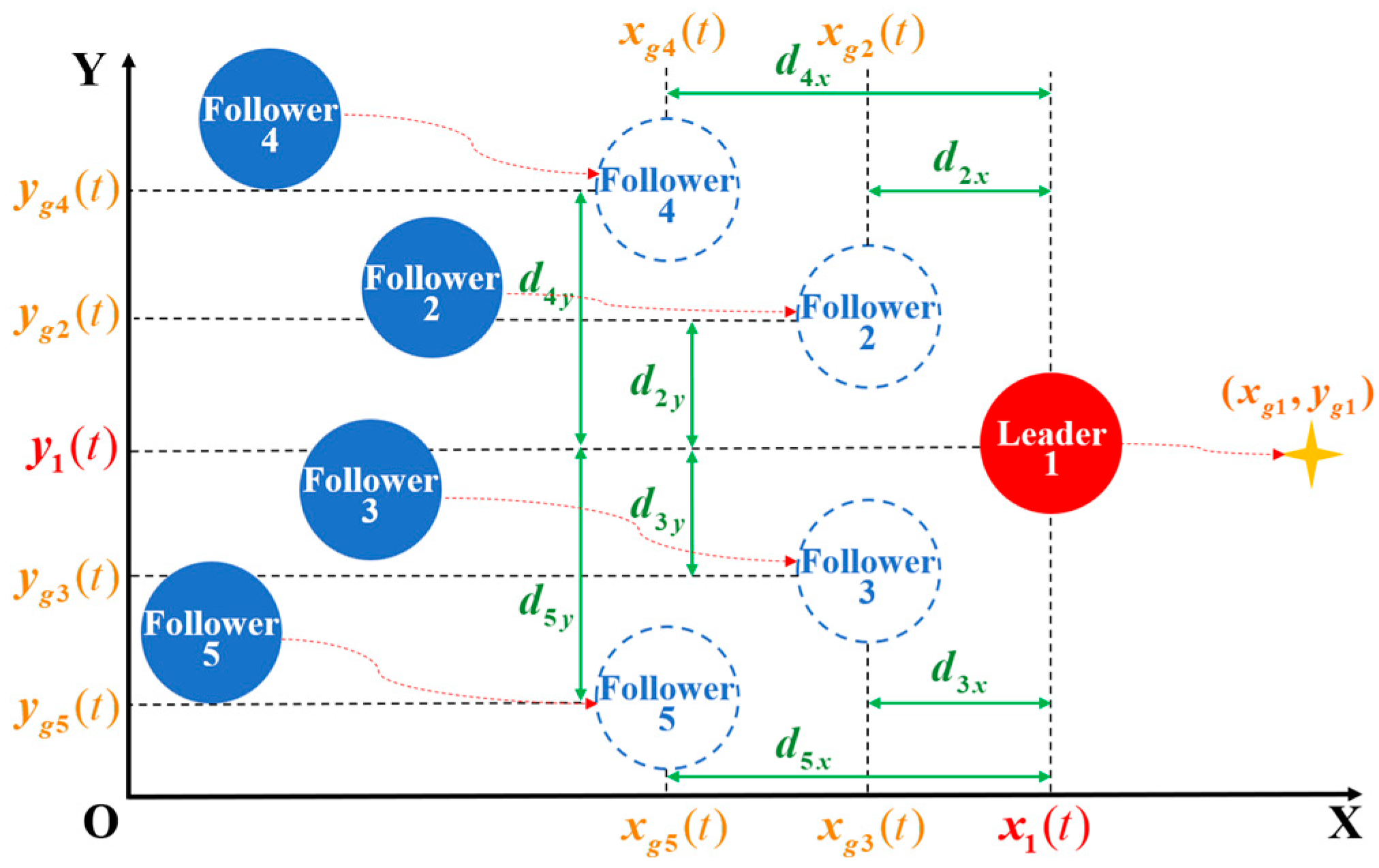
In this paper, Section 2 presents the dynamical modeling of the leader–follower formation adopted in our multi-UAV system. Section 3 introduces the fundamental principles of the traditional artificial potential field (APF) method, followed by detailed explanations of the proposed adaptive artificial potential field (AAPF) and its integration with the deflected simulated annealing (DSA) algorithm. Section 4 conducts simulation experiments and analyses in four scenarios: oscillation test, formation reconfiguration, obstacle avoidance in complex environments, and escape from semi-enclosed obstacles. The results demonstrate the feasibility and effectiveness of the proposed DSA-AAPF method. Finally, Section 5 summarizes the conclusions and discusses potential directions for future work.

2. Leader–Follower Formation Dynamics

2.1. Modeling of the Leader–Follower System

Consider a multi-UAV system comprising $n$ UAVs, where the dynamics of each UAV $i$ are modeled as follows:

$${\dot{\mathit{X}}}_i(t)={\mathit{u}}_i(t),i=1,\dots ,n$$

(1)

where ${\mathit{X}}_i(t)=\left[\begin{array}{l}{x}_i(t)\\ y_i(t)\end{array}\right],{\mathit{u}}_i(t)=\left[\begin{array}{l}{u}_{xi}(t)\\ u_{yi}(t)\end{array}\right]$, represent the position vector and control input (velocity) of UAV $i$ at time $t$, respectively.

A triangular formation structure is adopted, comprising one leader and four followers, as illustrated in Figure 1.

UAV 1 acts as the leader and is directed toward a predefined fixed target point $(x_{g1},y_{g1})$, thereby determining the trajectory of the entire formation. The remaining UAVs are designated as followers, whose actual positions are denoted by solid blue circles, while the dashed blue circles represent their desired positions within the formation. These desired positions dynamically change with respect to the leader’s location.

The relative displacement vector between follower $i$ and its corresponding virtual target is defined as:

$${\mathit{D}}_i=\left[\begin{array}{l}{d}_{ix}\\ d_{iy}\end{array}\right]=\left[\begin{array}{l}{x}_1(t)-x_{gi}(t)\\ y_1(t)-y_{gi}(t)\end{array}\right]$$

(2)

where ${\mathit{D}}_i$ is a predefined constant vector representing the intended offset between the leader and follower $i$ within the formation.

2.2. Graph-Theoretic Representation and Communication Topology

The communication among the UAVs is represented using graph theory. The multi-UAV network is modeled as an undirected graph $G=(N,E)$, where $N=\left\{e_1,e_2,\cdots ,e_n\right\}$ denotes the set of nodes (UAVs); $E=\left\{\left(e_i,e_j\right)\left|e_i,e_j\in N,i\ne j\right.\right\}$ denotes the set of undirected edges, each indicating a bidirectional communication link between a pair of UAVs, and $(e_i,e_j)$ denotes the communication of UAVs $i$ and $j$($i,j=1,2,\cdots ,n$).

An adjacency matrix $\mathit{A}(G)={[a_{ij}]}_{n\times n}$ is associated with graph $G$, where:

$$a_{ij}=\left\{\begin{array}{l}1,(i,j)\in E\\ 0,(i,j)\notin E\end{array}\right.$$

(3)

Each node’s degree is defined as the number of its direct neighbors. The degree matrix $\mathit{D}(G)=diag({\lambda }_1,{\lambda }_2,\cdots ,{\lambda }_n)$ is a diagonal matrix with entries ${\lambda }_i={\displaystyle {\sum }_{j=1}^n{a}_{ij}}$, and the Laplacian matrix of the graph is then defined as $\mathit{L}=\mathit{D}(G)-\mathit{A}(G)$.

3. Improved Artificial Potential Field Method

3.1. Fundamentals and Analysis of the Traditional Artificial Potential Field

The artificial potential field (APF) method was first introduced by Khatib, incorporating the concept of potential fields from physics into path planning. The core idea is to model the UAV as a point mass moving within a virtual force field, where the field comprises an attractive potential generated by the target and a repulsive potential induced by the surrounding obstacles. The resultant force acts as the driving input for the UAV’s motion.

The potential field function in the APF method is defined as the sum of the attractive and repulsive potential fields, as expressed in Equation (4):

$$\mathit{U}(\mathit{X}(t))={\mathit{U}}_{att}(\mathit{X}(t))+{\mathit{U}}_{rep}(\mathit{X}(t))$$

(4)

where $\mathit{X}(t)={(x_i(t),y_i(t))}^T$ denotes the position vector of the mobile robot, ${\mathit{U}}_{att}({\mathit{X}}_i(t))$ is the attractive potential field and ${\mathit{U}}_{rep}({\mathit{X}}_i(t))$ is the repulsive potential field, which are shown in Equations (5) and (6):

$${\mathit{U}}_{att}(\mathit{X}(t))={\displaystyle \frac{1}{2}}{k}_{att}\rho {(\mathit{X}(t),{\mathit{X}}_g)}^2$$

(5)

$${\mathit{U}}_{rep}(\mathit{X}(t))=\left\{\begin{array}{c}{\displaystyle \frac{1}{2}}{k}_{rep}{\left({\displaystyle \frac{1}{\rho (\mathit{X}(t),{\mathit{X}}_{obs})}}-{\displaystyle \frac{1}{{\rho }_0}}\right)}^2,\rho (\mathit{X}(t),{\mathit{X}}_{obs})<{\rho }_{\begin{array}{l}0\\ \end{array}}\\ 0,\rho (\mathit{X}(t),{\mathit{X}}_{obs})\ge {\rho }_0\end{array}\right.$$

(6)

where $k_{att}>0$ and $k_{rep}>0$ denote the attractive and repulsive gain coefficients, respectively; ${\mathit{X}}_g$ represents the goal position, and ${\mathit{X}}_{obs}$ denotes the nearest point on the obstacle surface to the UAV. For circular obstacles, this point corresponds to the intersection of the line connecting the UAV and the obstacle center with the obstacle boundary. The terms $\rho (\mathit{X}(t),{\mathit{X}}_g)$ and $\rho (\mathit{X}(t),{\mathit{X}}_{obs})$, respectively, denote the Euclidean distances of the UAV from the target point and the obstacle, and ${\rho }_0$ defines the maximum influence radius of the obstacle. Beyond this radius, the repulsive force exerted by the obstacle on the UAV is zero.

The artificial force applied to the UAV is defined as the negative gradient of the total potential field, consisting of both attractive and repulsive components. The resultant force experienced by UAV $i$ is expressed as:

$$\mathit{F}({\mathit{X}}_i(t))=-\nabla [\mathit{U}({\mathit{X}}_i(t))]={\mathit{F}}_{att}({\mathit{X}}_i(t))+{\mathit{F}}_{rep}({\mathit{X}}_i(t))$$

(7)

where the attractive force ${\mathit{F}}_{att}({\mathit{X}}_i(t))$ is:

$${\mathit{F}}_{att}(\mathit{X}(t))=-k_{att}(\mathit{X}(t)-{\mathit{X}}_g)$$

(8)

and the repulsive ${\mathit{F}}_{rep}({\mathit{X}}_i(t))$ is:

$${\mathit{F}}_{rep}({\mathit{X}}_i(t))=\left\{\begin{array}{c}{k}_{rep}\left({\displaystyle \frac{1}{\rho ({\mathit{X}}_i(t),{\mathit{X}}_{obs})}}-{\displaystyle \frac{1}{{\rho }_0}}\right){\displaystyle \frac{1}{\rho {({\mathit{X}}_i(t),{\mathit{X}}_{obs})}^2}}{\displaystyle \frac{\partial \rho ({\mathit{X}}_i(t),{\mathit{X}}_{obs})}{\partial {\mathit{X}}_i(t)}},\rho ({\mathit{X}}_i(t),{\mathit{X}}_{obs})<{\rho }_0\\ 0,\rho ({\mathit{X}}_i(t),{\mathit{X}}_{obs})\ge {\rho }_0\end{array}\right.$$

(9)

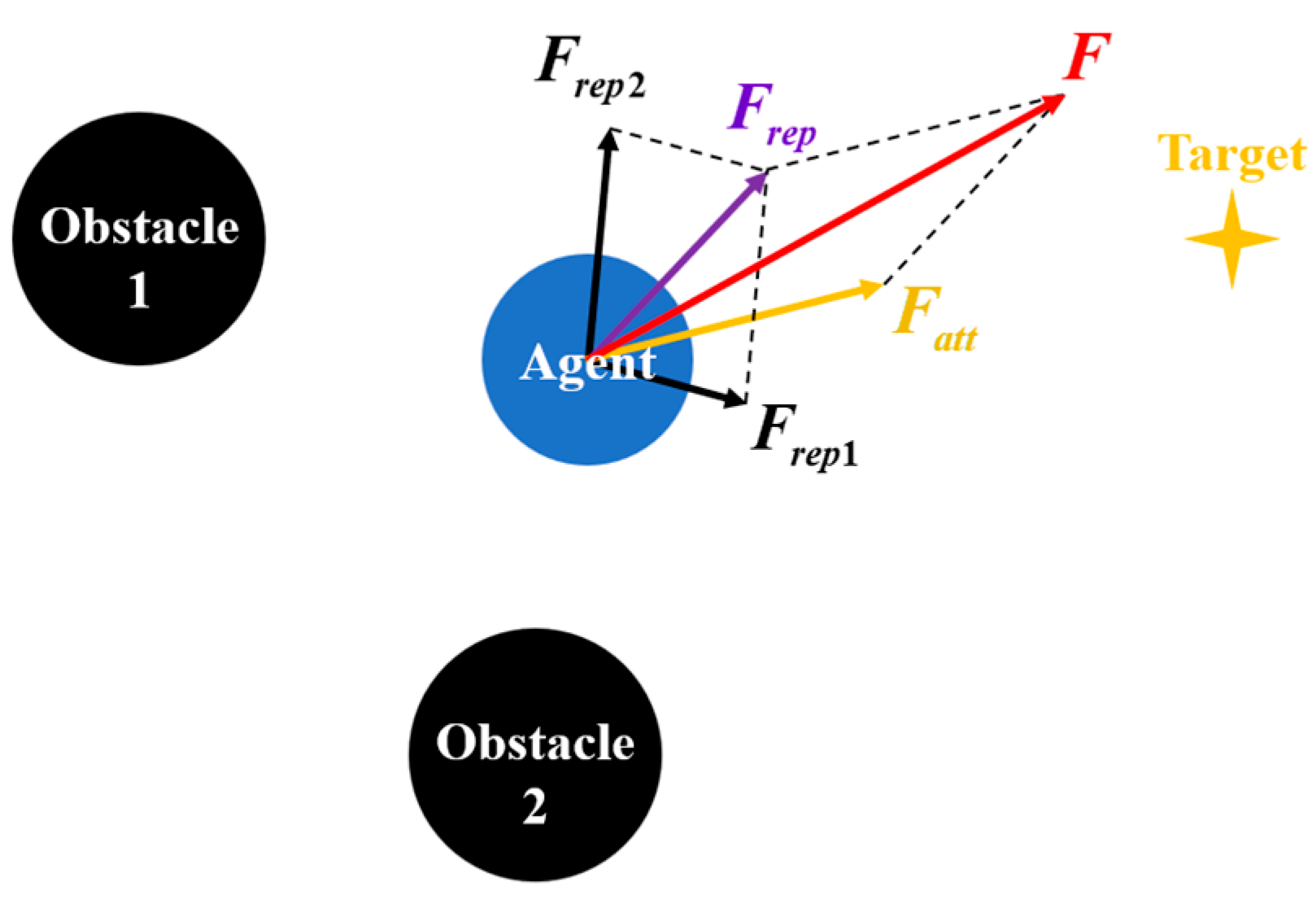
When multiple obstacles are present in the environment, the total repulsive force acting on a UAV is the superposition of the repulsive forces exerted by each obstacle. Accordingly, the resultant force acting on UAV $i$ is expressed as:

$$\mathit{F}({\mathit{X}}_i(t))={\mathit{F}}_{att}({\mathit{X}}_i(t))+{\displaystyle \sum _{j=1}^m{\mathit{F}}_{repj}({\mathit{X}}_i(t))}$$

(10)

where $m$ denotes the number of obstacles affecting the UAV.

An illustration of the force components under the APF framework is shown in Figure 2.

Despite its simplicity and computational efficiency, the traditional APF method suffers from several significant drawbacks.

(1) The attractive force in the conventional APF is linearly proportional to the distance between the UAV and the target. As a result, when the UAV is far from the target, it may move too rapidly, potentially leading to excessive acceleration toward obstacles. This sudden proximity to obstacles can induce large repulsive forces, causing oscillations or even collisions. Conversely, when the UAV is close to the target, the attraction becomes too weak, and the UAV may fail to reach the goal.

(2) To better mimic physical realism, recent implementations often constrain the UAVs to moving a fixed step length in the direction of the resultant force. However, such an approach neglects the magnitude of the resultant force, leading to slow convergence and reduced efficiency. Moreover, the final positioning accuracy becomes dependent on the fixed step size, limiting the precision–speed tradeoff.

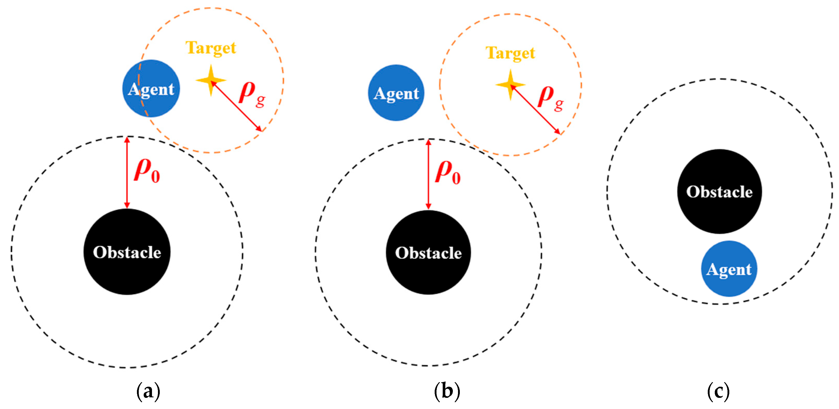
(3) The traditional APF framework is unable to handle local minima effectively. As illustrated in Figure 3, three typical scenarios may trap the UAV. In cases 1 and 2, the attractive and repulsive forces are nearly equal in magnitude but opposite in direction, resulting in oscillatory behavior or stagnation. In case 3, the UAV is confined within a U-shaped obstacle configuration, where the repulsive field completely blocks the path toward the goal, leaving the UAV unable to escape.

To overcome these limitations, this study proposes an improved APF framework within the context of a distributed leader–follower formation. The potential field function is redefined, and a momentum-inspired smoothing technique is introduced into the force computation to mitigate oscillations and ensure smooth trajectories. An adaptive attractive gain function is also designed to regulate the UAV’s velocity across different phases of its motion. Furthermore, to enable rapid reformation and precise convergence after obstacle avoidance, a fast-converging consensus controller is incorporated into the formation framework. Finally, a modified simulated annealing mechanism is developed to allow the UAVs to escape the local minima, particularly within semi-enclosed environments.

3.2. Adaptive Artificial Potential Field

3.2.1. Redefinition of the Potential Field Function

To improve upon the limitations of the classical APF, the potential field function is redefined in Equations (11) and (12) while retaining the basic structure as the sum of the attractive and repulsive components:

$${\mathit{U}}_{att}({\mathit{X}}_i(t))={\displaystyle \frac{1}{2}}{k}_{att}\rho {({\mathit{X}}_i(t),{\mathit{X}}_{gi}(t))}^2+{\displaystyle \frac{1}{2}}{k}_{att}{\displaystyle \sum _{j=1}^n{a}_{ij}}{({\mathit{X}}_i(t)-{\mathit{X}}_j(t)-({\mathit{D}}_i-{\mathit{D}}_j))}^2$$

(11)

$${\mathit{U}}_{rep}({\mathit{X}}_i(t))=\left\{\begin{array}{c}{\displaystyle \frac{1}{2}}{k}_{rep}{\left({\displaystyle \frac{1}{\rho ({\mathit{X}}_i(t),{\mathit{X}}_{obs})}}-{\displaystyle \frac{1}{{\rho }_0}}\right)}^2\rho {({\mathit{X}}_i(t),{\mathit{X}}_{gi}(t))}^b,\rho ({\mathit{X}}_i(t),{\mathit{X}}_{obs})<{\rho }_0\\ 0,\rho ({\mathit{X}}_i(t),{\mathit{X}}_{obs})\ge {\rho }_0\end{array}\right.$$

(12)

where ${\mathit{X}}_{gi}(t)=(x_{gi}(t),y_{gi}(t))$ denotes the virtual target point of UAV $i$. For the leader UAV (UAV 1), the target ${\mathit{X}}_{g1}=(x_{g1},y_{g1})$ is fixed and predefined. The vector ${\mathit{D}}_i=\left[\begin{array}{l}{d}_{ix}\\ d_{iy}\end{array}\right]=\left[\begin{array}{l}{x}_1(t)-x_{gi}(t)\\ y_1(t)-y_{gi}(t)\end{array}\right],i\ne 1$ represents the constant relative displacement between the leader and the follower in the desired formation. For the leader itself, ${\mathit{D}}_1=\left[\begin{array}{l}{d}_{1x}\\ d_{1y}\end{array}\right]=\left[\begin{array}{l}0\\ 0\end{array}\right]$. The term $\rho (\cdot )$ denotes the distance function between two points, and $b=0.9$ is a small positive constant to ensure the target is always at the minimum of the potential field.

The corresponding attractive and repulsive force functions are defined as:

$${\mathit{F}}_{att}({\mathit{X}}_i(t))=-k_{att}({\mathit{X}}_i(t)-{\mathit{X}}_{gi}(t))-k_{att}{\displaystyle \sum _{j\in N_i}{a}_{ij}({\mathit{X}}_i(t)-{\mathit{X}}_j(t)-({\mathit{D}}_i-{\mathit{D}}_j))}$$

(13)

$${\mathit{F}}_{rep}({\mathit{X}}_i(t))=\left\{\begin{array}{c}{\mathit{F}}_{rep1}({\mathit{X}}_i(t))+{\mathit{F}}_{rep2}({\mathit{X}}_i(t)),\rho ({\mathit{X}}_i(t),{\mathit{X}}_{obs})<{\rho }_0\\ 0,\rho ({\mathit{X}}_i(t),{\mathit{X}}_{obs})\ge {\rho }_0\end{array}\right.$$

(14)

Specifically, the repulsive terms ${\mathit{F}}_{rep1}({\mathit{X}}_i(t))$ and ${\mathit{F}}_{rep2}({\mathit{X}}_i(t))$ are expressed as:

$${\mathit{F}}_{rep1}({\mathit{X}}_i(t))=k_{rep}\left({\displaystyle \frac{1}{\rho ({\mathit{X}}_i(t),{\mathit{X}}_{obs})}}-{\displaystyle \frac{1}{{\rho }_0}}\right){\displaystyle \frac{1}{\rho {({\mathit{X}}_i(t),{\mathit{X}}_{obs})}^2}}{\displaystyle \frac{\partial \rho ({\mathit{X}}_i(t),{\mathit{X}}_{obs})}{\partial {\mathit{X}}_i(t)}}\rho {({\mathit{X}}_i(t),{\mathit{X}}_{gi}(t))}^b$$

(15)

$${\mathit{F}}_{rep2}({\mathit{X}}_i(t))=-{\displaystyle \frac{b}{2}}{k}_{rep}{\left({\displaystyle \frac{1}{\rho ({\mathit{X}}_i(t),{\mathit{X}}_{obs})}}-{\displaystyle \frac{1}{{\rho }_0}}\right)}^2{\displaystyle \frac{\partial \rho ({\mathit{X}}_i(t),{\mathit{X}}_{gi}(t))}{\partial {\mathit{X}}_i(t)}}\rho {({\mathit{X}}_i(t),{\mathit{X}}_{gi}(t))}^{b-1}$$

(16)

The resultant force in the AAPF retains the same form as the original APF expression shown in Equation (10).

3.2.2. Resultant Force Optimizes Momentum Smoothing

To address the issue of oscillations caused by abrupt repulsion near obstacles, a momentum-inspired smoothing mechanism is incorporated into the resultant force computation. Drawing on the momentum-based gradient descent, the current effective force is defined as a weighted combination of the current and previous timestep forces:

$${\mathit{F}}^{\prime }({\mathit{X}}_i(t))=\alpha \mathit{F}({\mathit{X}}_i(t-\Delta t))+(1-\alpha )\mathit{F}({\mathit{X}}_i(t))$$

(17)

where $\mathit{F}({\mathit{X}}_i(t))$ is the raw resultant force at time $t$, computed from Equations (10), (13), and (14); $\mathit{F}({\mathit{X}}_i(t-\Delta t))$ is the effective force from the previous timestep; and $\alpha \in [0,1]$ is a tunable coefficient controlling the momentum contribution.

Figure 4 illustrates the effect of the force smoothing, as defined in Equation (17). In Figure 4a, which depicts the case without smoothing, the blue dashed circle, solid blue circle, and red dashed circle represent the positions of the UAV at three successive timesteps. At the intermediate timestep, the UAV approaches the obstacle too closely due to the strong attractive force. This results in a large repulsive reaction force from the obstacle, which sharply redirects the UAV and causes a sudden deviation from its intended path—leading to the position indicated by the red dashed circle.

In contrast, Figure 4b demonstrates the scenario with force smoothing applied. Although the UAV reaches a similar position near the obstacle, the momentum-based adjustment prevents it from being forcefully repelled. As a result, the UAV maintains a smooth trajectory and navigates around the obstacle without abrupt direction changes.

3.2.3. Adaptive Attractive Gain Design

To address the limitations of the traditional artificial potential field—namely, that UAVs tend to move too quickly when far from the target due to excessive attractive forces (leading to potential collisions) and too slowly when approaching the target due to insufficient attraction (resulting in failure to reach the goal)—an adaptive attractive gain function $k_{att}(\cdot )$ is proposed. The gain is defined in a piecewise manner to regulate the UAV’s motion across different phases of the trajectory, as shown in Equation (18):

$$k_{atti}=\left\{\begin{array}{c}{h}_i{k}_{att0},{\mathit{F}}_{req}({\mathit{X}}_i(t))=0and\rho ({\mathit{X}}_t(t),{\mathit{X}}_{gi}(t))<{\rho }_g\\ {\displaystyle \frac{{\tau }_i{k}_{att0}}{\rho ({\mathit{X}}_t(t),{\mathit{X}}_{gi}(t))+\delta }},{\mathit{F}}_{req}({\mathit{X}}_t(t))=0and\rho ({\mathit{X}}_t(t),{\mathit{X}}_{gi}(t))\ge {\rho }_g\\ k_{att0},{\mathit{F}}_{req}({\mathit{X}}_i(t))\ne 0\end{array}\right.$$

(18)

where $k_{att0}>0$ is a constant baseline gain; $\delta =1.0\times {10}^{-8}$ is a small positive constant introduced to prevent division by zero and to stabilize the numerical computation; and $h_i\ge 1$, ${\tau }_i\ge 1$ and ${\rho }_g>0$ are tunable constants that can be selected according to the performance requirements.

The three operational cases are illustrated in Figure 5.

In Figure 5a, when the UAV is not influenced by any obstacle and is within the specified proximity threshold ${\rho }_g$ from the goal, the attractive gain is set to a moderate value $h_i{k}_{att0}$. This setting ensures that the UAV does not overshoot the target due to high speed while maintaining sufficient pull to prevent stagnation near the goal. In Figure 5b, if the UAV is outside the goal proximity but still free from repulsive influence, the attractive gain is scaled inversely with respect to the distance to the goal using the adaptive attractive gain term ${\displaystyle \frac{{\tau }_i{k}_{att0}}{\rho ({\mathit{X}}_t(t),{\mathit{X}}_{gi}(t))+\delta }}$. A larger value of $\tau$ amplifies the gain in this mid-range zone, accelerating the UAV’s movement toward the goal after obstacle avoidance, thereby shortening the convergence time. In Figure 5c, when the UAV is within the repulsive influence of an obstacle, the attractive gain is held at $k_{att0}$, promoting cautious and stable movement around the obstacle.

3.2.4. Control Law

The controller employed in this study is based on a consensus control framework proposed by Huang [33], which supports different convergence performance requirements. The framework includes multiple control functions with fast convergence guarantees and proven stability. In this work, a set of nine control functions is selected from the original framework and applied to the AAPF-based formation structure. The simulation results in Section 4 demonstrate that this controller, when integrated with the proposed formation control algorithm, enables rapid reconfiguration and accurate convergence after obstacle avoidance.

The control input for UAV $i$ is defined as follows:

$${\mathit{u}}_i(t)={\gamma }_{i}s({\mathit{F}}^{\prime }({\mathit{X}}_i(t)))\varphi (\left|{\mathit{F}}^{\prime }({\mathit{X}}_i(t))\right|),i=1,2,\dots ,n$$

(19)

where ${\gamma }_i$ is a gain coefficient; $s(\cdot )$ is a direction function determining the control orientation and stability; and $\varphi (\cdot )$ is a shaping function designed to meet performance criteria such as the convergence speed and robustness.

The vector $\left|\mathit{F}\prime ({\mathit{X}}_i(t))\right|={(\left|{\mathit{F}}_x^{\prime }({\mathit{X}}_i(t))\right|,\left|{\mathit{F}}_y^{\prime }({\mathit{X}}_i(t))\right|)}^T$ denotes the smoothed resultant force at time $t$.

3.3. Escape from Semi-Enclosed Obstacles Using DSA-AAPF

This subsection introduces an enhanced approach for escaping local minima by combining the deflected simulated annealing (DSA) algorithm with the adaptive artificial potential field (AAPF) framework. The discussion focuses primarily on scenarios involving semi-enclosed obstacles.

Simulated annealing (SA) is a Monte-Carlo-based probabilistic optimization algorithm used for approximating global optima. The algorithm consists of two nested loops: an outer loop in which the system temperature gradually decreases and an inner loop that probabilistically accepts new candidate solutions based on the metropolis criterion. The probability that a particle reaches equilibrium at a given temperature $T$ is $\exp (-\Delta E/(kT))$, where $E$ is the internal energy at temperature $T$, $\Delta E$ represents the change in energy between states, and $k$ is the Boltzmann constant. The metropolis acceptance rule is formally defined as:

$$p=\left\{\begin{array}{l}\exp \left(-{\displaystyle \frac{E({\mathit{X}}_n)-E({\mathit{X}}_0)}{T}}\right),E({\mathit{X}}_n)>E({\mathit{X}}_0)\\ 1,E({\mathit{X}}_n)\le E({\mathit{X}}_0)\end{array}\right.$$

(20)

where ${\mathit{X}}_n$ is a candidate position at the next iteration; ${\mathit{X}}_0$ is the current position of the UAV; $E({\mathit{X}}_n)$ and $E({\mathit{X}}_0)$ represent the internal energy (i.e., the potential field value) at these respective positions; and $T$ denotes the current system temperature.

The temperature is updated iteratively according to a linear decay model as follows:

$$T(t)=\beta T(t-\Delta t)$$

(21)

where $\beta \in (0,1)$ is a decay constant slightly less than one.

When applied to the AAPF-based path-planning framework, the variables in Equation (20) correspond to the following:

(1) ${\mathit{X}}_0={\mathit{X}}_i(t)$: the UAV’s current position;

(2) ${\mathit{X}}_n={\mathit{X}}_i(t+\Delta t)$: a randomly sampled candidate position nearby;

(3) $E({\mathit{X}}_0)=U({\mathit{X}}_i(t))$: the potential energy at the current position;

(4) $E({\mathit{X}}_n)=U({\mathit{X}}_i(t+\Delta t))$: the potential energy at the candidate position.

The key improvement proposed in this study lies in the method used to generate the candidate points ${\mathit{X}}_i(t+\Delta t)$, particularly in the context of escaping from semi-enclosed obstacles.

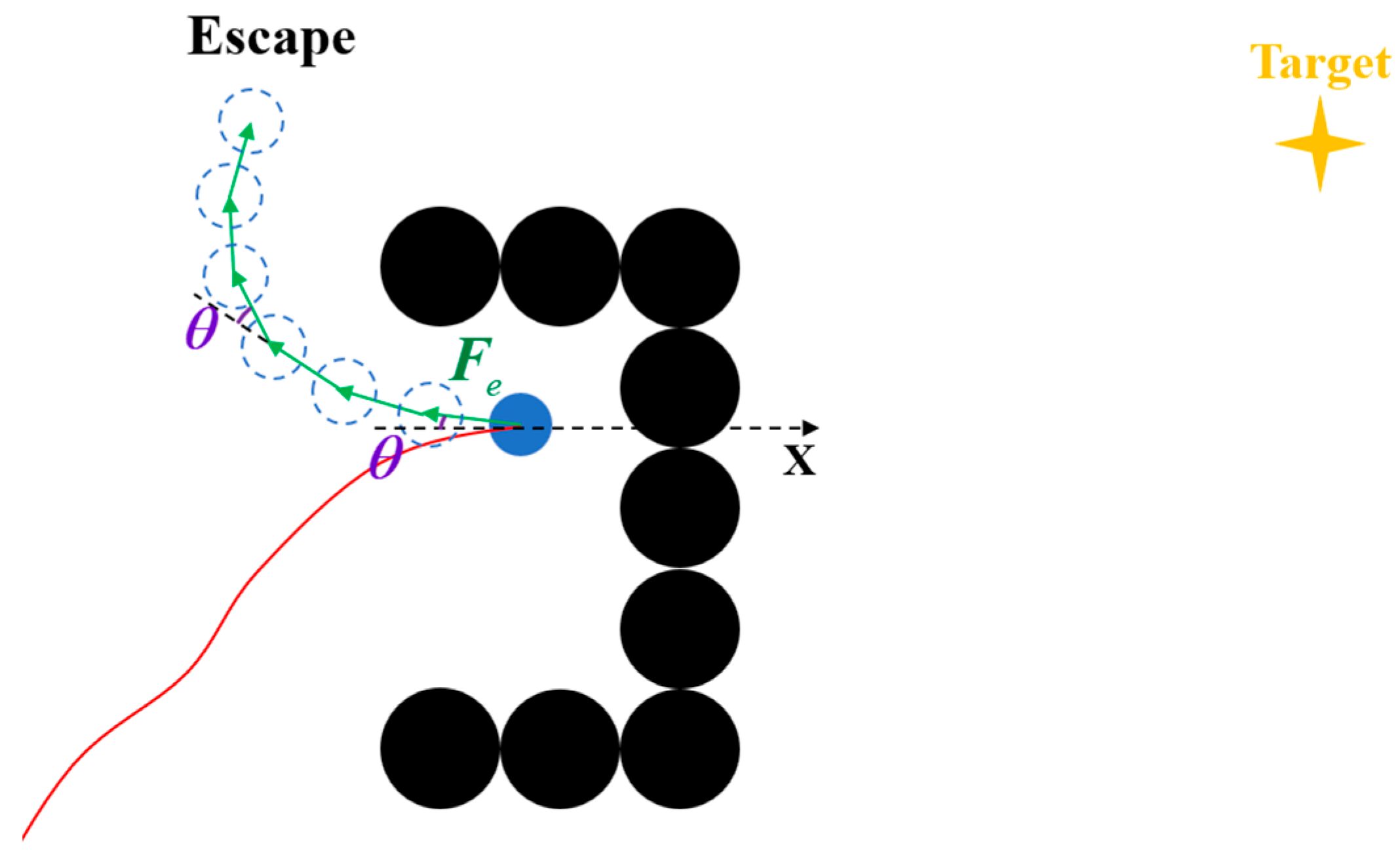
As illustrated in Figure 6, the red solid line represents the trajectory previously traversed by the UAV, while the blue filled circle indicates the UAV’s current position. When the UAV becomes trapped in a local minimum within a semi-enclosed obstacle, a constant-magnitude force ${\mathit{F}}_e$ is applied. This force is rotated by a random angle within a predefined range in a consistent direction over multiple iterations, generating an arc-like trajectory that enables the UAV to escape the enclosure.

To realize this escape mechanism, three key issues must be addressed.

(1) Directional Ambiguity

Within a semi-enclosed obstacle, there are typically two feasible escape directions. Choosing the correct direction significantly reduces the travel distance to the goal. As shown in Figure 7, following the direction indicated by the green path yields a faster and more direct route to the goal compared to the orange path. Therefore, determining the optimal escape direction is critical.

(2) Parameter Design for Force and Rotation

The magnitude of the escape force ${\mathit{F}}_e$ and the rotational angle $\theta$ must be carefully selected. If the force is too weak or the rotation too large, the UAV may fail to exit the enclosure or collide with the obstacle boundary.

(3) Escape Condition Determination

A reliable method must be defined to determine when the UAV has successfully exited the semi-enclosed obstacle.

To address these challenges, the following strategy is proposed.

It is first noted that in real scenarios, it is rare for the attractive and repulsive forces to exactly cancel each other out in magnitude and direction. Instead, local minima usually occur when these forces are nearly equal and opposite, resulting in a net force that is too small to drive motion. When such a situation arises within a semi-enclosed obstacle, it is observed that eliminating the attraction component often leaves a repulsive force pointing outward—i.e., in a direction favorable for escape.

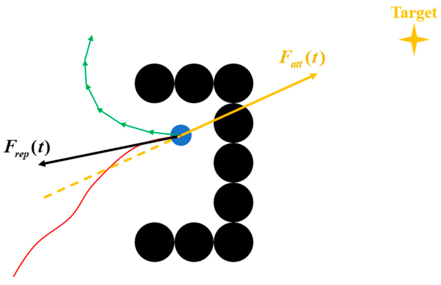
Additionally, since the goal is usually located outside the obstacle, the attractive force tends to bias the UAV toward that side. As a result, when the UAV enters the enclosure and becomes trapped, the repulsive force vector typically lies on the same side as the extension of the attractive force’s opposite direction. This relationship is illustrated in Figure 8, where the optimal escape direction lies on the opposite side of the attractive force vector.

In the proposed algorithm, the escape direction is determined by identifying which side of the extended line opposite the attractive force the repulsive force lies on, as illustrated in Figure 9. In this figure, the blue arrow represents the vector difference ${\mathit{F}}_{att}({\mathit{X}}_i(t))-{\mathit{F}}_{rep}({\mathit{X}}_i(t))$. The angle ${\theta }_a$ denotes the angle between the attractive force direction and the positive x-axis, while ${\theta }_b$ represents the angle between the vector ${\mathit{F}}_{att}({\mathit{X}}_i(t))-{\mathit{F}}_{rep}({\mathit{X}}_i(t))$ and the positive x-axis.

If ${\theta }_a>{\theta }_b$, the UAV should rotate in the clockwise direction.

If ${\theta }_a<{\theta }_b$, the UAV should rotate counterclockwise.

Next, let $t_s$ denote the time at which the UAV enters a local minimum. The repulsive force experienced at this moment, ${\mathit{F}}_{rep}({\mathit{X}}_i(t_s))$, is defined as the initial value of the escape force ${\mathit{F}}_e$, denoted as ${\mathit{F}}_e({\mathit{X}}_i(t_s))$. The angle between ${\mathit{F}}_{rep}({\mathit{X}}_i(t_s))$ and ${\mathit{F}}_{att}({\mathit{X}}_i(t_s))$ is denoted as ${\theta }_c$, where $0<{\theta }_c<\pi$. The value of angle $\theta$ is picked randomly in section ($0,{\theta }_c-{\displaystyle \frac{\pi }{c}}]$, where $c>{\displaystyle \frac{\pi }{{\theta }_c}}$ is a predefined constant.

The rotation matrix is defined as:

$$R(\theta )=\left\{\begin{array}{l}\left[\begin{array}{cc}\cos \theta & \sin \theta \\ -\sin \theta & \cos \theta \end{array}\right],{\theta }_a>{\theta }_b\\ \left[\begin{array}{cc}\cos \theta & -\sin \theta \\ \sin \theta & \cos \theta \end{array}\right],{\theta }_a<{\theta }_b\end{array}\right.$$

(22)

The escape force ${\mathit{F}}_e({\mathit{X}}_i(t_s+\Delta t))$ at time $t_s+\Delta t$ is then updated as:

$${\mathit{F}}_e({\mathit{X}}_i(t_s+\Delta t))=\mathit{R}(\theta ){\mathit{F}}_e({\mathit{X}}_i(t_s))$$

(23)

As a result, this force ${\mathit{F}}_e({\mathit{X}}_i(t_s))$ is applied iteratively, rotating by $\theta$ at each step, maintained at a constant magnitude, until the UAV successfully escapes the semi-enclosed obstacle

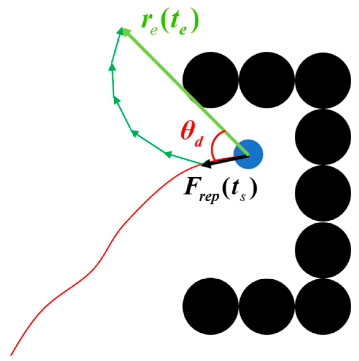
Let $t_e$ denote the final iteration time of the simulated annealing loop. As illustrated in Figure 10, $r_e(t_e)$ represents the displacement vector from the local minimum position to the UAV’s position at time $t_e$. The angle ${\theta }_d$ denotes the angle between $r_e(t_e)$ and the initial escape force ${\mathit{F}}_{rep}({\mathit{X}}_i(t_s))$, which is equivalent to ${\mathit{F}}_e({\mathit{X}}_i(t_s))$. In the algorithm, a threshold angle ${\theta }_0$ is defined as a constant in $[{\displaystyle \frac{\pi }{3}},{\displaystyle \frac{2\pi }{3}}]$. If ${\theta }_d\ge {\theta }_0$, the UAV is considered to have successfully escaped from the semi-enclosed obstacle.

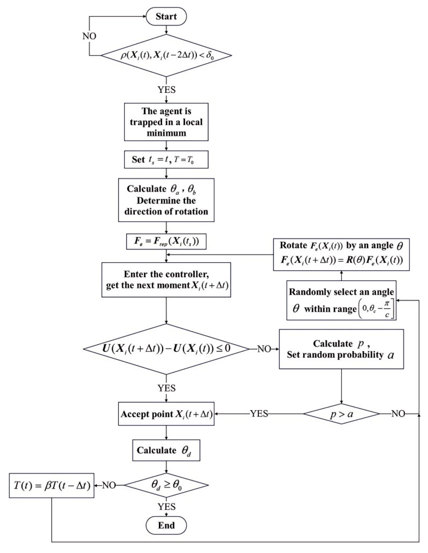
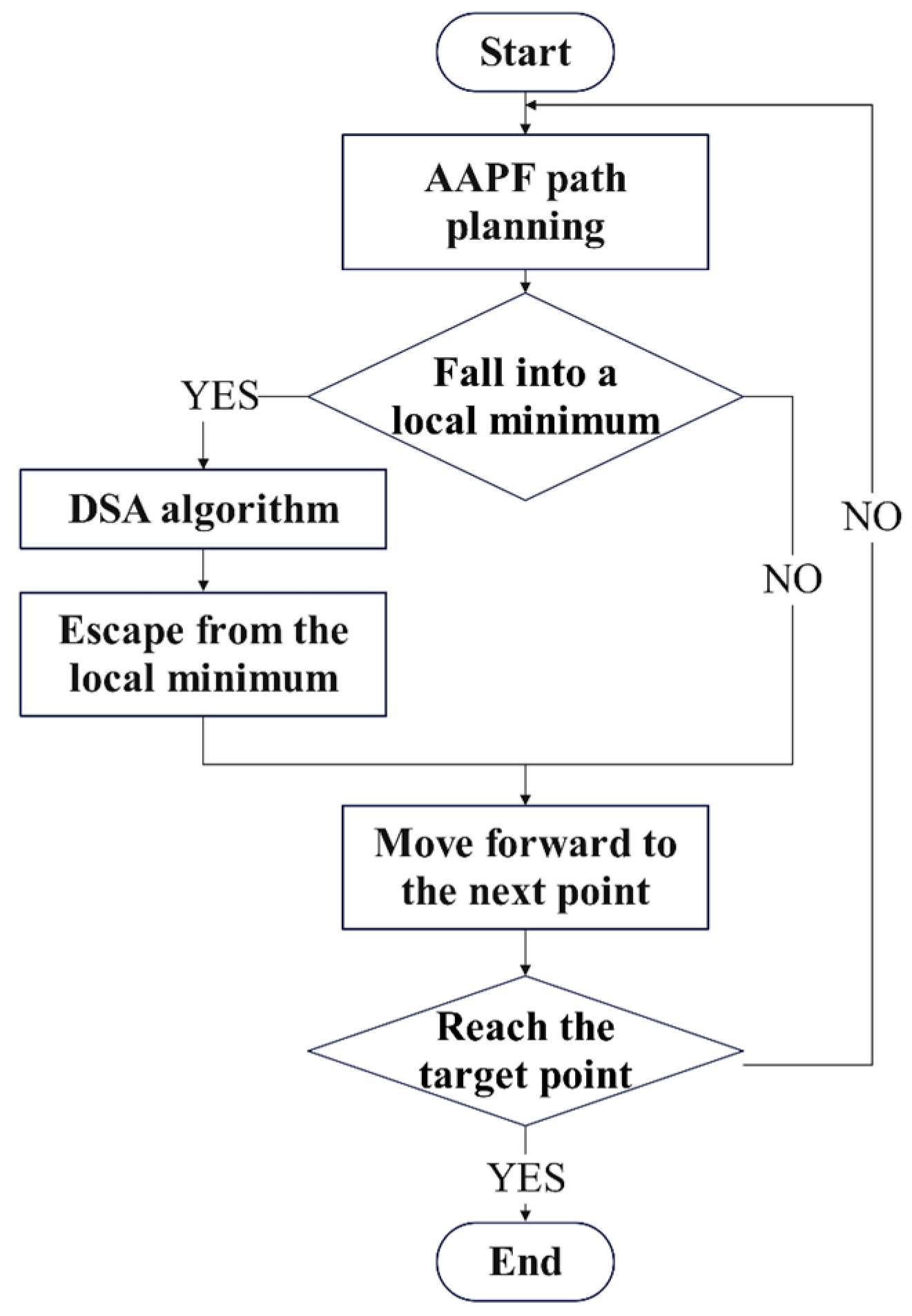
The complete procedure of the improved simulated annealing algorithm is summarized in Figure 11. The flowchart of the whole DSA-AAPF algorithm is shown in Figure 12.

4. Algorithm Simulations and Performance Evaluation

To validate the effectiveness of the proposed algorithm, a series of simulation experiments are conducted focusing on four core capabilities: (1) oscillatory testing of the resultant force optimization effects; (2) reformation of the multi-UAV formation after obstacle evasion; (3) obstacle avoidance when the environment is complicated; and (4) escaping from semi-enclosed obstacle environments. The controller functions employed are selected from nine function pairs proposed by Huang [33], as listed in

Table 2. Control function combinations used for the performance evaluation.

Group	$\mathit{s}(\mathit{z})$	$\mathit{\varphi }(\left|\mathit{z}\right|)$
(1)	$sign(\mathit{z})$	$\left|\mathit{z}\right|$
	$5\left(\left|\mathit{z}+0.1\right|-\left|\mathit{z}-0.1\right|\right)$	$\left|\mathit{z}\right|$
	${\displaystyle \frac{\mathit{z}}{\left(\left|\mathit{z}\right|+0.1\right)}}$	$\left|\mathit{z}\right|$
(2)	$sign(\mathit{z})$	$2{\left|\mathit{z}\right|}^{0.5}$
	$5\left(\left|\mathit{z}+0.1\right|-\left|\mathit{z}-0.1\right|\right)$	$2{\left|\mathit{z}\right|}^{0.5}$
	${\displaystyle \frac{\mathit{z}}{\left(\left|\mathit{z}\right|+0.1\right)}}$	$2{\left|\mathit{z}\right|}^{0.5}$
(3)	$sign(\mathit{z})$	$2{\left|\mathit{z}\right|}^{0.5}+2{\left|\mathit{z}\right|}^{1.5}$
	$5\left(\left|\mathit{z}+0.1\right|-\left|\mathit{z}-0.1\right|\right)$	$2{\left|\mathit{z}\right|}^{0.5}+2{\left|\mathit{z}\right|}^{1.5}$
	${\displaystyle \frac{\mathit{z}}{\left(\left|\mathit{z}\right|+0.1\right)}}$	$2{\left|\mathit{z}\right|}^{0.5}+2{\left|\mathit{z}\right|}^{1.5}$

Note: In this table and the subsequent analysis, the variable $z$ is used as a shorthand notation for the force vector ${\mathit{F}}^{\prime }({\mathit{X}}_t(t))$.

. The performance metrics are evaluated based on the convergence speed and accuracy of each UAV along the $x$ and $y$ axes, ultimately identifying the most suitable controller configuration for the subsequent experiments.

The subsequent simulations are designed to assess the effectiveness of the formation navigation in environments with multiple complex obstacles, focusing on the avoidance performance and convergence efficiency. Finally, the capability of the formation to escape from semi-enclosed traps is tested to verify the robustness of the deflected simulated annealing–adaptive artificial potential field (DSA-AAPF) algorithm.

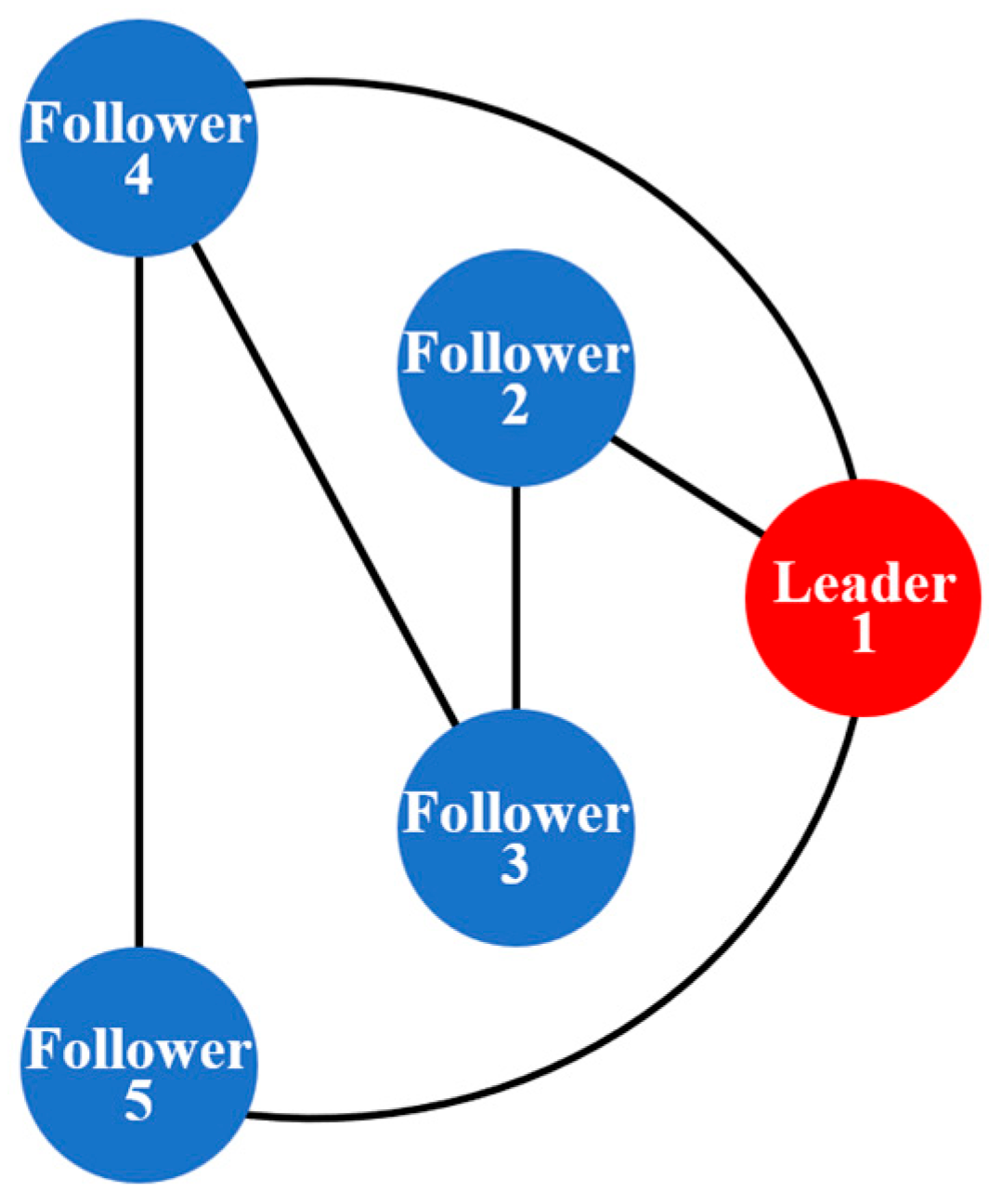
A formation composed of five UAVs is used for the evaluation, in which UAV 1 serves as the leader and the remaining four act as followers. The communication topology is modeled as an undirected graph, as shown in Figure 13, where the adjacency matrix satisfies $a_{12}=a_{14}=a_{15}=a_{23}=a_{34}=a_{45}=1$, with all the other elements set to zero. The controller gain parameters are configured as follows: ${\gamma }_1=1$, ${\gamma }_2=3$, ${\gamma }_3=5$, ${\gamma }_4=3$, ${\gamma }_5=3$, and the formation spacing vectors are defined as: ${\mathit{D}}_2=\left[\begin{array}{c}1\\ -1\end{array}\right]$, ${\mathit{D}}_3=\left[\begin{array}{c}1\\ 1\end{array}\right]$, ${\mathit{D}}_4=\left[\begin{array}{c}2\\ -2\end{array}\right]$, ${\mathit{D}}_5=\left[\begin{array}{c}2\\ 2\end{array}\right]$.

4.1. Oscillation Test

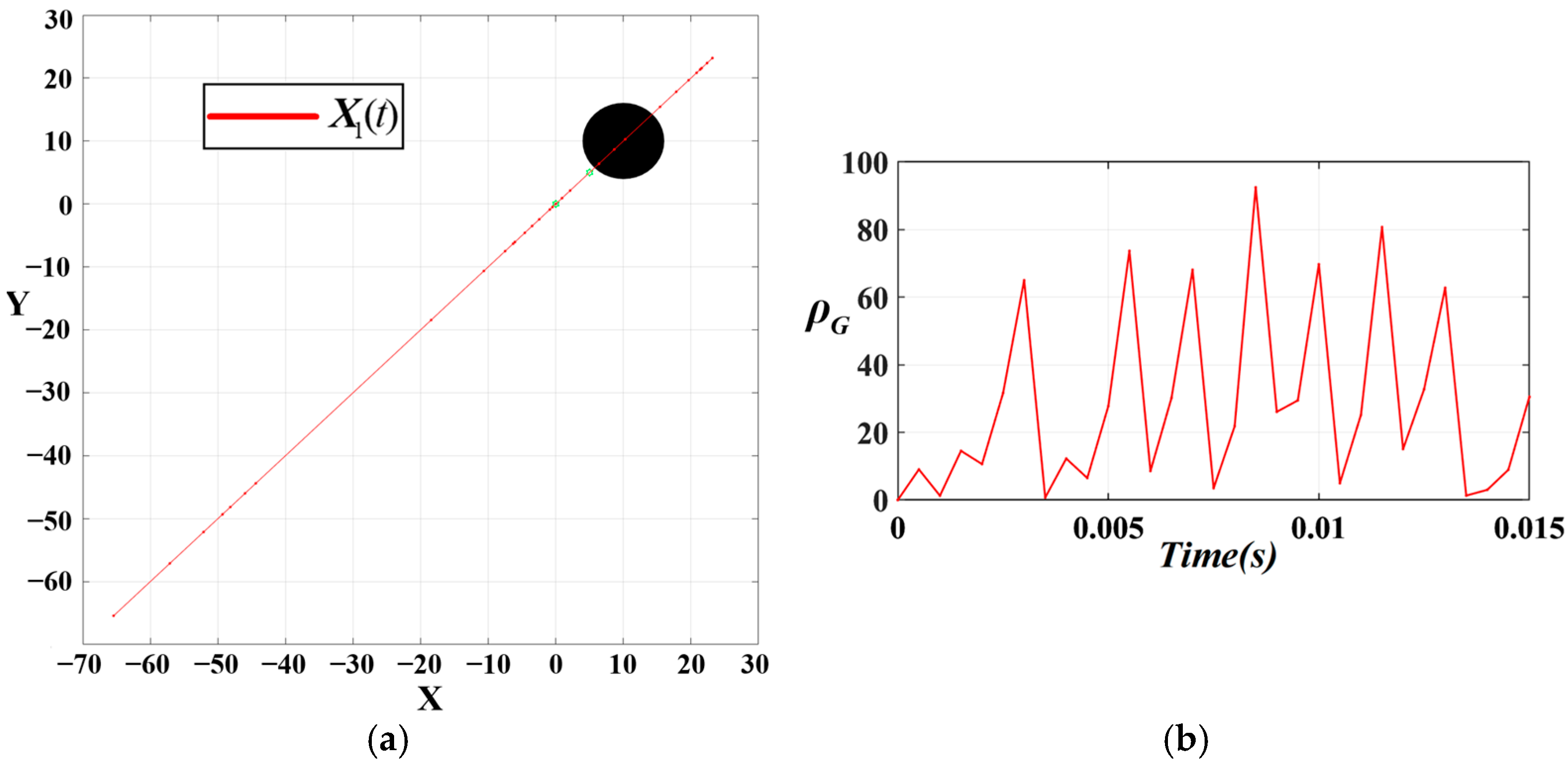
In order to obtain the scaling parameter $\alpha$ in the resultant force optimization in Equation (17), we set the obstacles and target points very close to each other and three points co-linear with the starting point of the UAV to create an environment where the UAV would oscillate back and forth for the oscillation test. The magnitude of the scaling parameter $\alpha$ is adjusted to observe the degree of suppression of the oscillations by the Equation (17) resultant force optimizes momentum smoothing in 0.015 $s$. The distance of the UAV from the starting point is defined as ${\rho }_G$.

Only one UAV is used in the test, with the starting point ${\mathit{X}}_1(0)={(0,0)}^T$, the target point ${\mathit{X}}_{g1}={(5,5)}^T$, and a circular obstacle centered at ${(10,10)}^T$. The attractive gain is set as $k_{att0}=18$, and the repulsive gain as $k_{rep}=4$.

It is found experimentally that the best suppression of the oscillations is achieved when the scaling parameter is $\alpha =0.6$. The simulated path diagram with the variation of ${\rho }_G$ when $\alpha =0$ is shown in Figure 14.

From Figure 14, the UAV is displaced by a large distance due to the excessive gravitational force and then is too close to the obstacle to generate a large resistance and reverse the displacement by a large distance, with the variance of ${\rho }_G$ reaching 741.5648, generating a very pronounced oscillation and even causing the path point to pass through the obstacle.

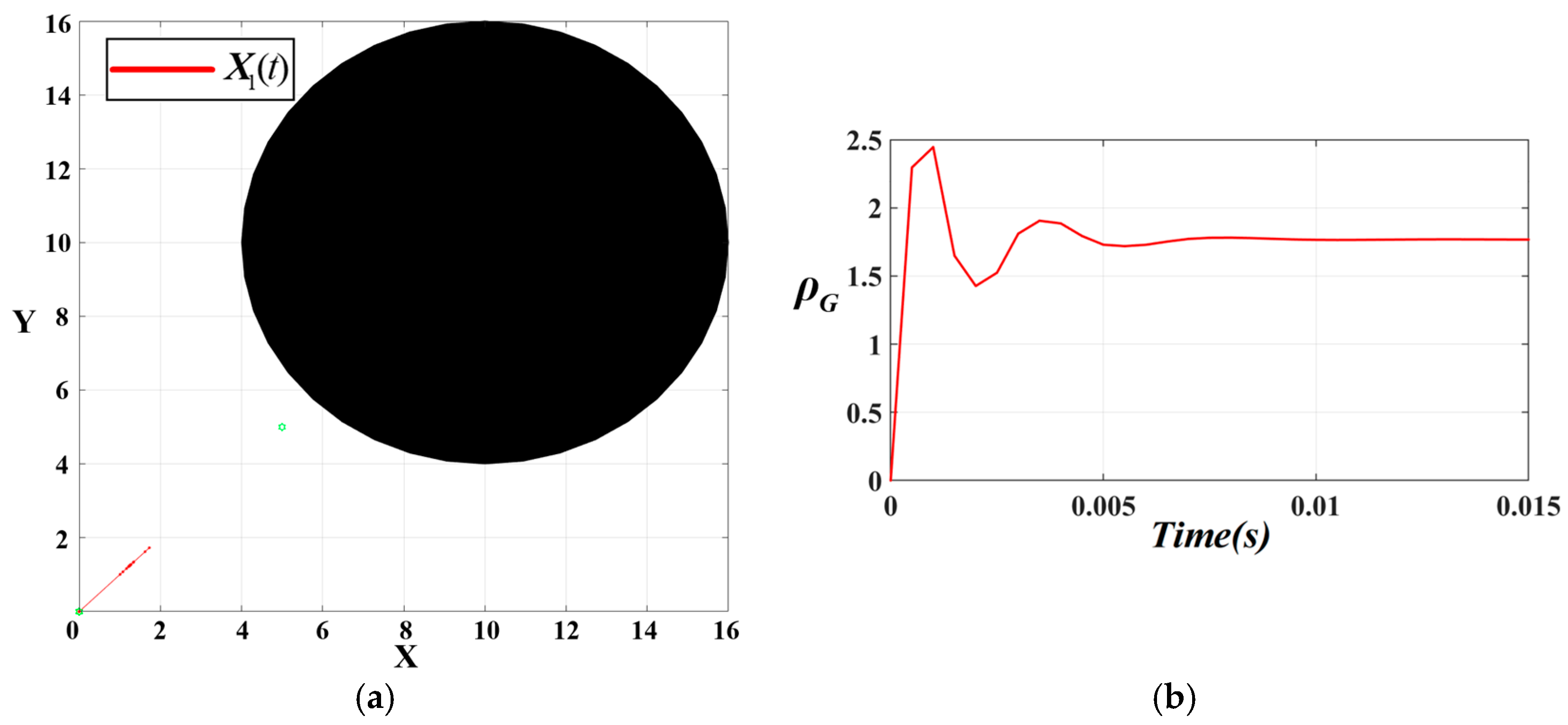
The simulated path diagram with the variation of ${\rho }_G$ when the resultant force optimization is used and $\alpha =0.6$ is shown in Figure 15.

From Figure 15, the oscillation phenomenon of the UAV in Figure 14 is very significantly suppressed, with a variance of only 0.1353. Under the same conditions, after the UAV is optimized with a resultant force of $\alpha =0.6$, no very large oscillation occurs and the equilibrium is restored within 0.01 $s$.

To summarize, for our subsequent experiments, we selected $\alpha =0.6$.

4.2. Formation Reconfiguration Test

To assess the system’s ability to maintain the formation structure during obstacle avoidance and reformation, the deviation between the UAV’s position and its target is quantified as ${\mathit{e}}_i(t)=\left[\begin{array}{l}{e}_{xi}(t)\\ e_{yi}(t)\end{array}\right]={\mathit{X}}_i(t)-{\mathit{X}}_{gi}(t)$. A circular obstacle is placed on the UAV’s trajectory to observe the response behavior. The attractive gain parameters are configured as $h_1=13$, $h_2=h_3=h_4=h_5=1.7$, and the adaptive gain factors ${\tau }_1=27$, ${\tau }_2={\tau }_3={\tau }_4={\tau }_5=4$. The obstacle’s influence radius is set as ${\rho }_g=0.2$. The initial positions are specified as ${\mathit{X}}_1(0)={(1,11)}^T$,${\mathit{X}}_2(0)={(1,16)}^T$, ${\mathit{X}}_3(0)={(1,4)}^T$, ${\mathit{X}}_4(0)={(1,21)}^T$, and ${\mathit{X}}_5(0)={(1,1)}^T$. The leader’s destination is defined as ${\mathit{X}}_{g1}={(50,11)}^T$, with a circular obstacle centered at ${(25,11)}^T$. It is defined that when $\left|e_{xi}(t)\right|<0.1\mathrm{and}\left|e_{yi}(t)\right|<0.1,i=2,3,4,5$, to maintain the formation state, the error between the positions of all the followers and the formation target in the $x$ and $y$ directions must not exceed 0.1. Define time $t_{rec}$ as the time it takes for a UAV formation to start avoiding obstacles from maintaining the formation state, leaving the formation state, bypassing the obstacles, and then resuming maintaining the formation state.

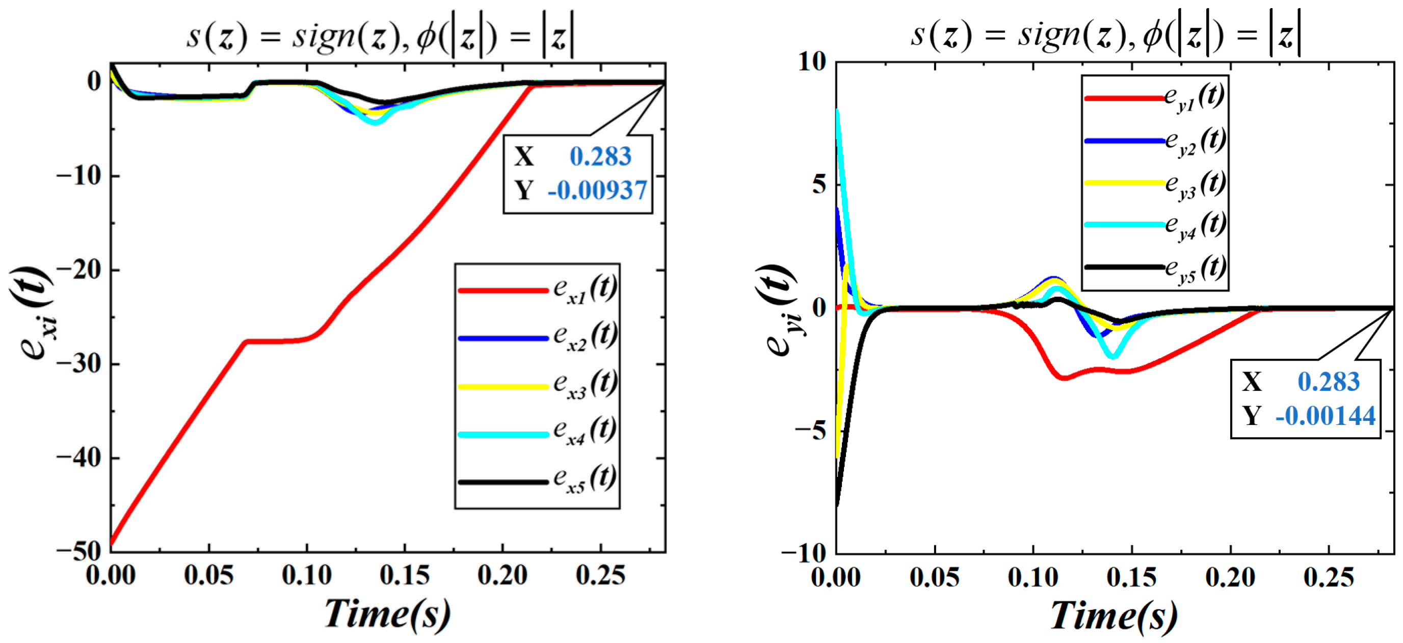
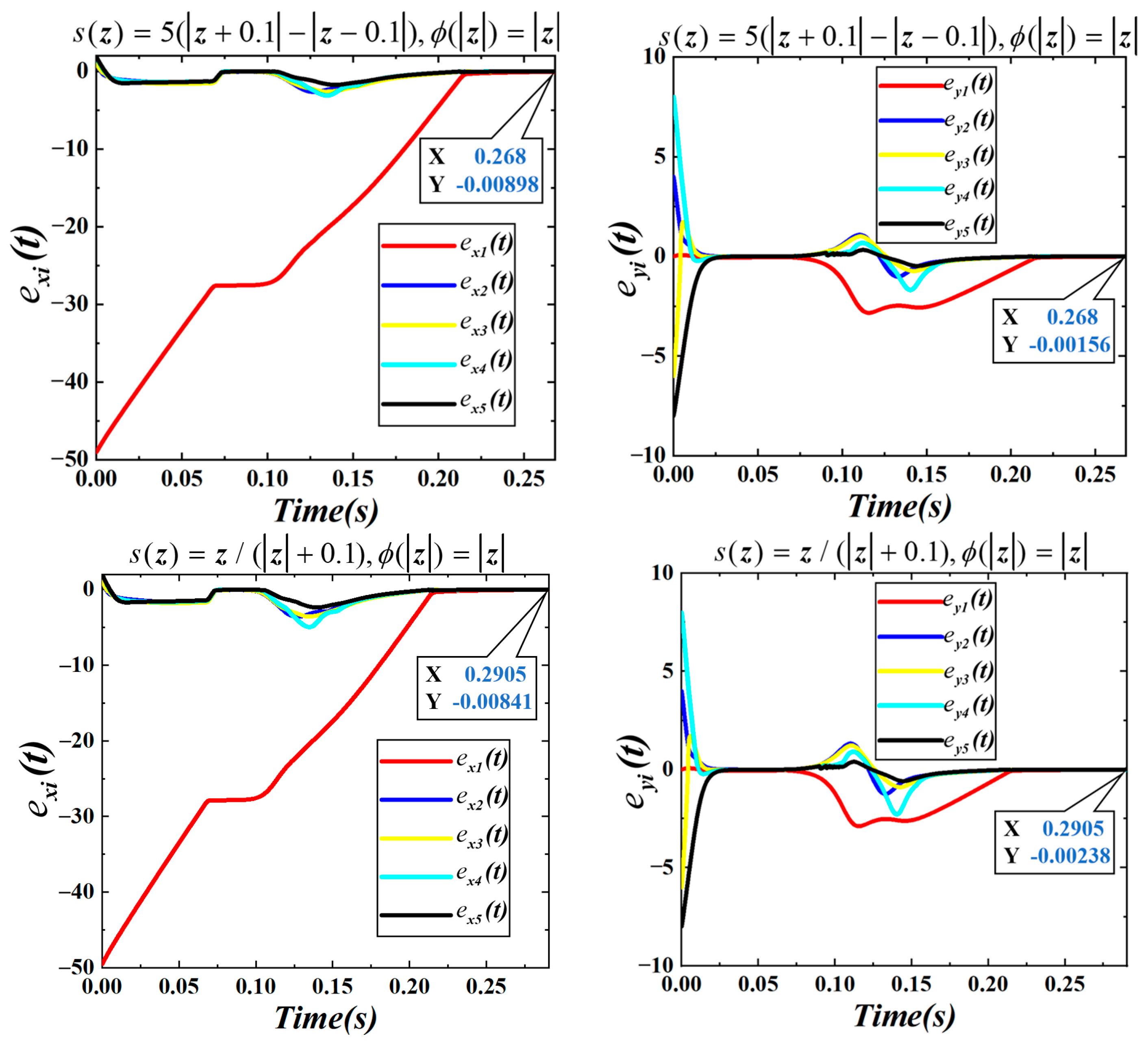
Given the structural similarity among the three configurations in each group (due to the identical potential functions), only one simulation formation trajectory per group is visualized.

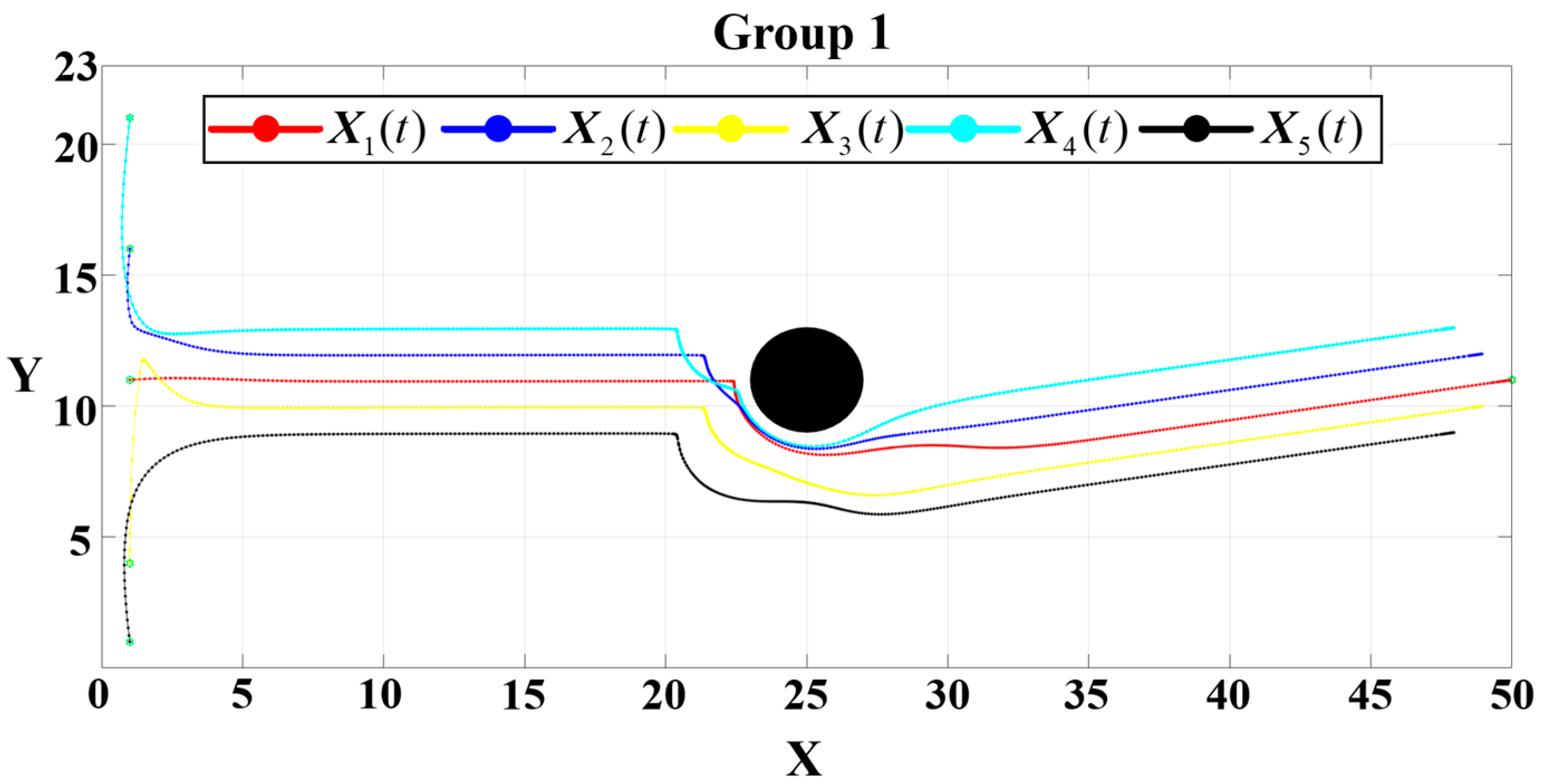
For Group 1, the attractive gain is set as $k_{att0}=13$, and the repulsive gain as $k_{rep}=5$. The corresponding trajectory of the formation reconfiguration and obstacle avoidance is depicted in Figure 16, while the convergence dynamics in the $x$ and $y$ directions are illustrated in Figure 17.

From the results shown in Figure 16, the UAV formation maintains a compact structure during the initial phase of motion. Upon encountering the obstacle, the formation disperses to perform obstacle avoidance and subsequently reassembles into the predefined configuration before converging to the target destination.

As indicated in Figure 17, $t_{rec}$ under the three controllers is 0.124 $s$, 0.113 $s$, and 0.132 $s$, respectively, and the final distance to the target point converges to a very small value. The total completion times for the three configurations are approximately 0.283 $s$, 0.268 $s$, and 0.2905 $s$, respectively.

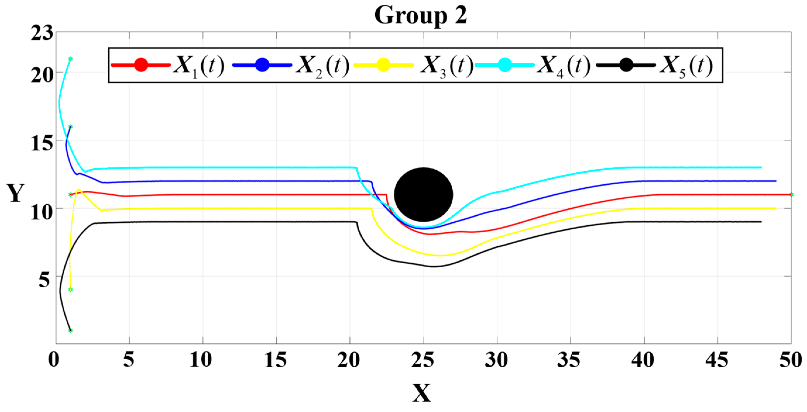
In the simulations for Group 2, the parameters are adjusted to $k_{att0}=38$ and $k_{rep}=10$. The obstacle avoidance and reformation trajectory is presented in Figure 18, while the convergence dynamics in the $x$ and $y$ directions are illustrated in Figure 19.

The simulation reveals a stable reformation process similar to that of Group 1; however, the higher attractive gain caused a marginal increase in the oscillatory motion during avoidance. Despite this, the UAVs successfully completed the formation restoration with comparable convergence accuracy. $t_{rec}$ under the three controllers is 0.324 $s$, 0.286 $s$, and 0.337 $s$. The time required to complete the task for the three cases is approximately 0.885 $s$, 0.864 $s$, and 0.887 $s$, respectively.

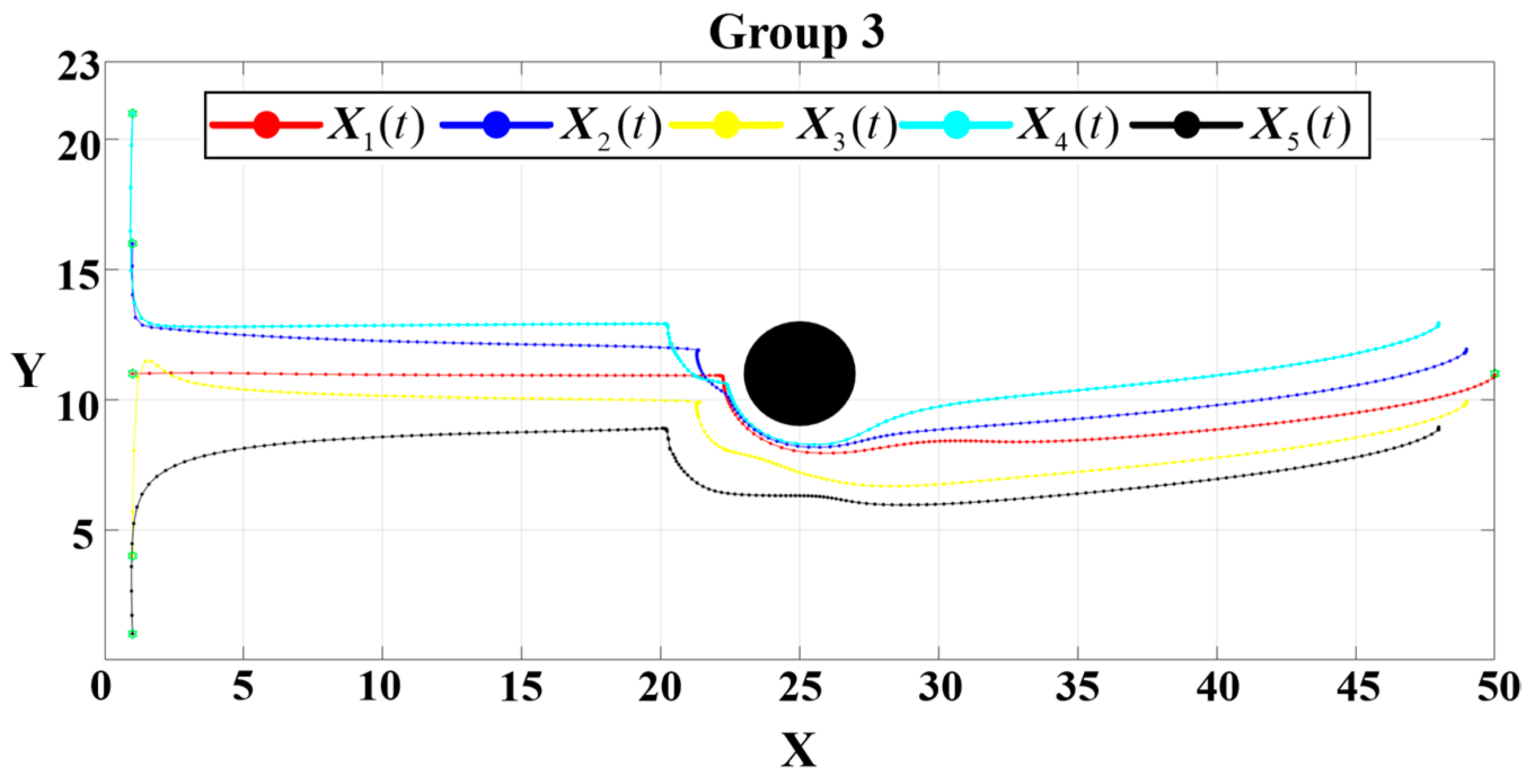
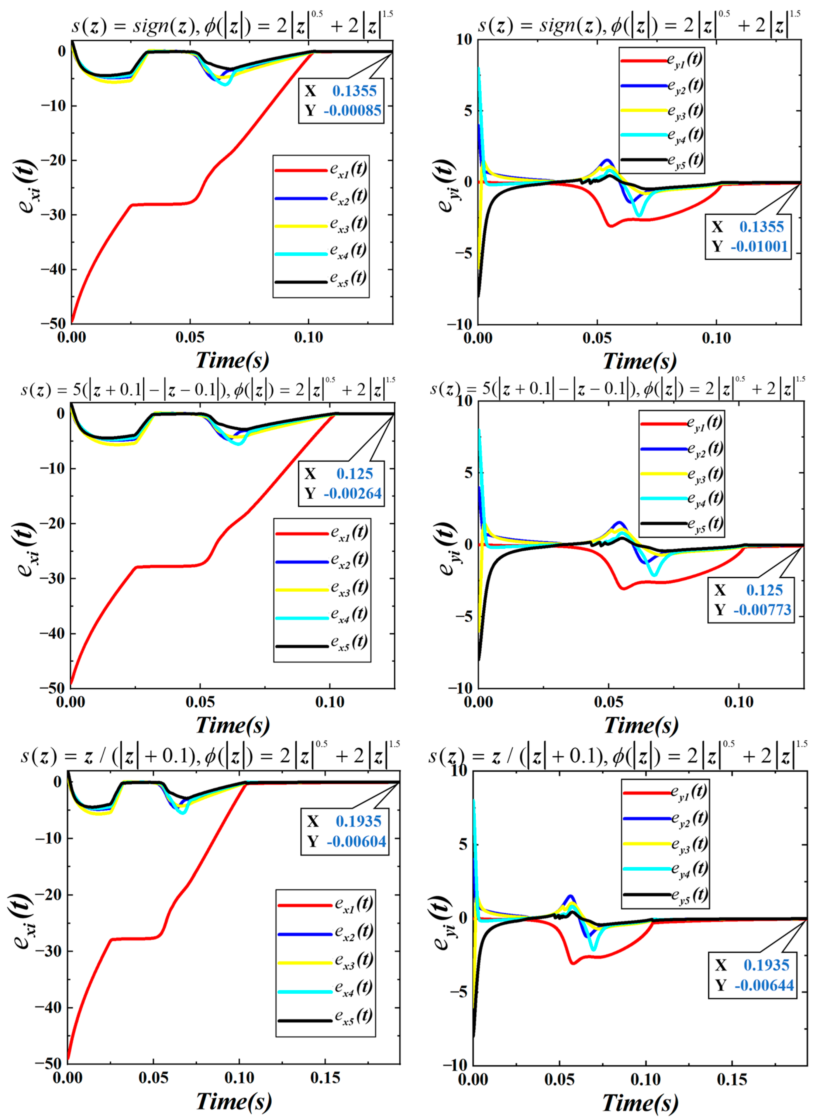
For Group 3, the gains are configured as $k_{att0}=3$ and $k_{rep}=3$. The obstacle avoidance behavior is illustrated in Figure 20, while the convergence dynamics in the $x$ and $y$ directions are illustrated in Figure 21.

From Figure 21, $t_{rec}$ under the three controllers is 0.064 $s$, 0.052 $s$, and 0.075 $s$. Subsequently, the positional deviations from the target point converge to negligible values. The total completion times for the three scenarios are 0.1355 $s$, 0.125 $s$, and 0.1935 $s$, respectively.

As summarized in

Table 3. Performance comparison of the three group configurations.

Group	Function	${\mathit{t}}_{\mathit{r}\mathit{e}\mathit{c}}$	${\mathit{t}}_{\mathit{e}\mathit{n}\mathit{d}}$	${({\mathit{e}}_{\mathit{x}\mathit{i}}({\mathit{t}}_{\mathit{e}\mathit{n}\mathit{d}}),{\mathit{e}}_{\mathit{y}\mathit{i}}({\mathit{t}}_{\mathit{e}\mathit{n}\mathit{d}}))}^{\mathit{T}}$
(1)	$s(\mathit{z})=sign(\mathit{z}),\varphi (\left|\mathit{z}\right|)=\left|\mathit{z}\right|$	0.124 $s$	0.283 $s$	${(-0.00937,-0.00144)}^T$
	$s(\mathit{z})=5(\left|\mathit{z}+0.1\right|-\left|\mathit{z}-0.1\right|),\varphi (\left|\mathit{z}\right|)=\left|\mathit{z}\right|$	0.113 $s$	0.268 $s$	${(-0.00898,-0.00156)}^T$
	$s(\mathit{z})={\displaystyle \frac{\mathit{z}}{(\left|\mathit{z}\right|+0.1)}},\varphi (\left|\mathit{z}\right|)=\left|\mathit{z}\right|$	0.132 $s$	0.2905 $s$	${(-0.00841,-0.00238)}^T$
(2)	$s(\mathit{z})=sign(\mathit{z}),\varphi (\left|\mathit{z}\right|)=2{\left|\mathit{z}\right|}^{0.5}$	0.324 $s$	0.8855 $s$	${(-0.00936,-0.00013)}^T$
	$s(\mathit{z})=5(\left|\mathit{z}+0.1\right|-\left|\mathit{z}-0.1\right|),\varphi (\left|\mathit{z}\right|)=2{\left|\mathit{z}\right|}^{0.5}$	0.286 $s$	0.864 $s$	${(-0.00931,-0.00017)}^T$
	$s(\mathit{z})={\displaystyle \frac{\mathit{z}}{(\left|\mathit{z}\right|+0.1)}},\varphi (\left|\mathit{z}\right|)=2{\left|\mathit{z}\right|}^{0.5}$	0.337 $s$	0.887 $s$	${(-0.01002,-0.00001)}^T$
(3)	$s(\mathit{z})=sign(\mathit{z}),\varphi (\left|\mathit{z}\right|)=2{\left|\mathit{z}\right|}^{0.5}+2{\left|\mathit{z}\right|}^{1.5}$	0.064 $s$	0.1355 $s$	${(-0.00085,-0.01001)}^T$
	$s(\mathit{z})=5(\left|\mathit{z}+0.1\right|-\left|\mathit{z}-0.1\right|),\varphi (\left|\mathit{z}\right|)=2{\left|\mathit{z}\right|}^{0.5}+2{\left|\mathit{z}\right|}^{1.5}$	0.052 $s$	0.125 $s$	${(-0.00264,-0.00773)}^T$
	$s(\mathit{z})={\displaystyle \frac{\mathit{z}}{(\left|\mathit{z}\right|+0.1)}},\varphi (\left|\mathit{z}\right|)=2{\left|\mathit{z}\right|}^{0.5}+2{\left|\mathit{z}\right|}^{1.5}$	0.075 $s$	0.1935 $s$	${(-0.00604,-0.00644)}^T$

, while the configurations in Group 3 exhibit slightly inferior accuracy in the $y$ direction compared to Groups 1 and 2, it demonstrates superior convergence accuracy in the $x$ direction. Moreover, Group 3 consistently achieves faster reformation times and shorter total completion durations. Notably, the second configuration in Group 3 achieves the shortest overall completion time (0.125 $s$) while maintaining a high level of accuracy. When compared with conventional methods, this approach demonstrates significant improvements in both speed and precision. Consequently, this configuration—defined by $s(z)=5(\left|z+0.1\right|-\left|z-0.1\right|)$ and $\varphi (\left|z\right|)=2{\left|z\right|}^{0.5}+2{\left|z\right|}^{1.5}$—is selected for the subsequent simulations.

In order to evaluate the superiority of DSA-AAPF more intuitively, we next test the traditional APF algorithms in the same experimental environment as in the previous section for comparison. We categorize the traditional APF algorithms into the following two types depending on the UAV movement method.

(1) Movement with the resultant force as the control input (APF-F)

Instead of using the control rate, adaptive gain and control rate of the DSA-AAPF algorithm, only the resultant force is computed as a control input to move.

(2) Movement with a fixed step size in the direction of the resultant force (APF-S)

The difference from APF-F is that it does not move through the control input. Instead, it calculates the direction of the resultant force and then moves a fixed step in this direction, with a fixed step size of 0.1.

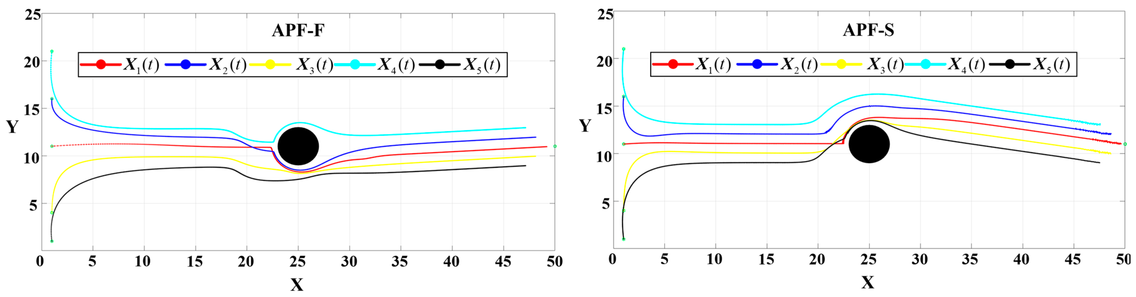
The gain of the control function used in the DSA-AAPF algorithm selected in the previous test is $k_{att0}=3$ and $k_{rep}=3$. Since the gravitational force acting on APF-F is too small at this gain and it is almost impossible to move in the second half, we increase the gravitational gain by four times and use $k_{att}=12$ and $k_{rep}=3$. The simulated formation path diagram of APF-F and APF-S is shown in Figure 22. The convergence dynamics in the $x$ and $y$ directions are illustrated in Figure 23.

From Figure 22, for the APF-S algorithm, when the UAV moves near the obstacles, an oscillation phenomenon occurs, resulting in an unbalanced path. This is because the resistance near the obstacles is relatively large and varies greatly with the position. Moving in a fixed step size causes the resultant force direction to oscillate back and forth at a large angle, thereby causing the oscillation of the UAV. For the APF-S algorithm, the UAV also experiences an oscillation phenomenon when approaching the target point. This is because when approaching the target point, the gravitational force exerted by the navigator on the target point is too small, while in the distributed control, part of the gravitational force exerted by the follower on the navigator causes the direction of the resultant force acting on the navigator to not always point toward the target point, resulting in an oscillation change. These oscillation phenomena prove that the APF-S algorithm is not applicable to the formation control of multiple UAVs.

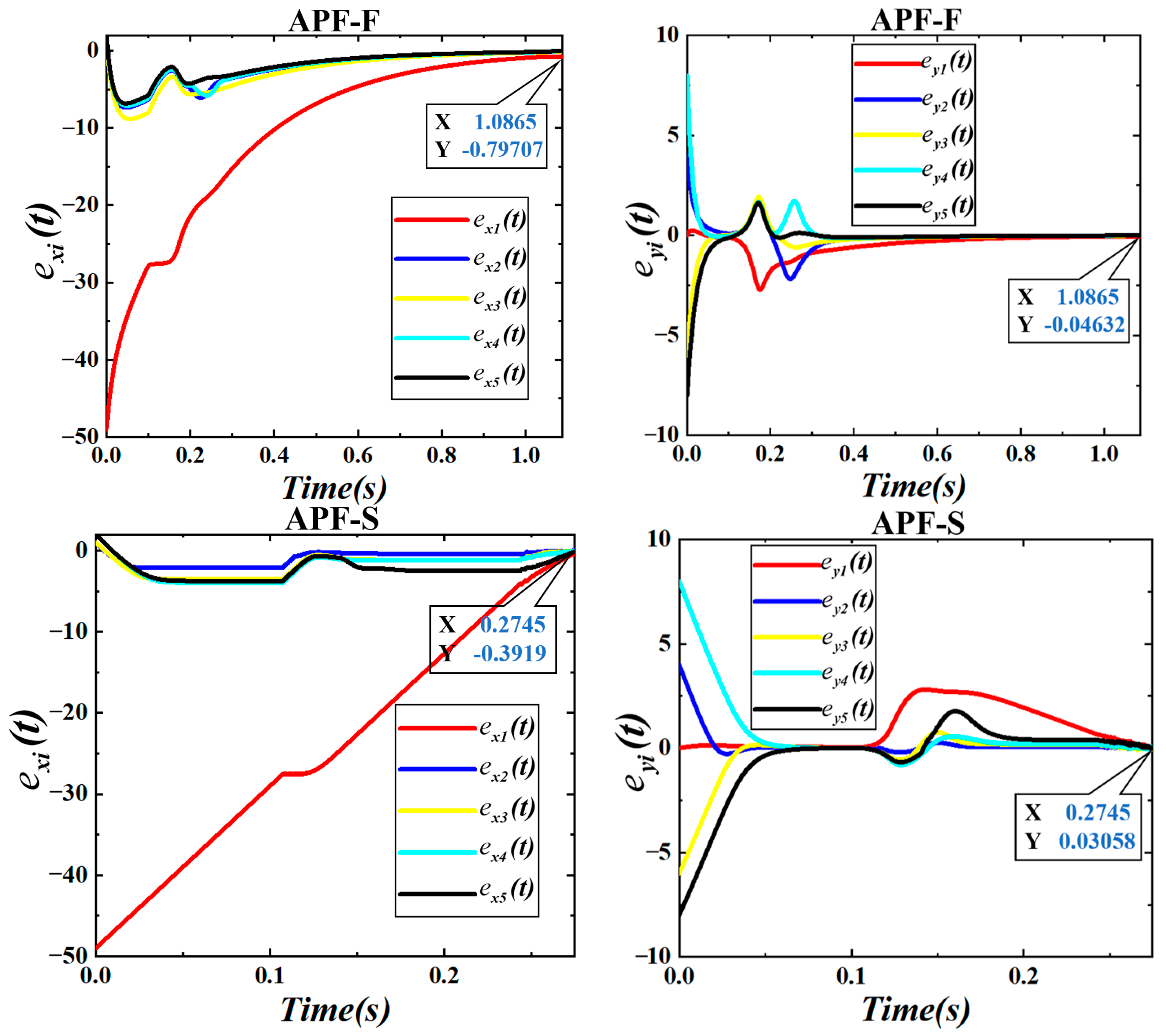
From Figure 23, APF-F is unable to enter the formation holding state before encountering obstacles due to its too slow convergence speed. Moreover, when approaching the target point, the convergence speed drops rapidly because the gravitational force becomes smaller and smaller. Under the APF-S algorithm, $t_{rec}=0.153s$. The total time taken by the two methods is 1.0865 $s$ and 0.2745 $s$, respectively, and eventually, they fail to converge to smaller values in the x direction, which are −0.79707 and −0.3919, respectively.

From

Table 4. The comparison between DSA-AAPF, APF-F and APF-S.

Algorithm	${\mathit{t}}_{\mathit{r}\mathit{e}\mathit{c}}$	${\mathit{t}}_{\mathit{e}\mathit{n}\mathit{d}}$	${({\mathit{e}}_{\mathit{x}\mathit{i}}({\mathit{t}}_{\mathit{e}\mathit{n}\mathit{d}}),{\mathit{e}}_{\mathit{y}\mathit{i}}({\mathit{t}}_{\mathit{e}\mathit{n}\mathit{d}}))}^{\mathit{T}}$
DSA-AAPF	0.052 $s$	0.125 $s$	${(-0.00264,-0.00773)}^T$
APF-F	Failure	1.0865 $s$	${(-0.79707,-0.04632)}^T$
APF-S	0.153 $s$	0.2745 $s$	${(-0.3919,-0.03058)}^T$

, DSA-AAPF far exceeds the traditional APF-F and APF-S algorithms in both the convergence speed and accuracy, and it can be well applied in multi-UAV formations.

4.3. Obstacle Avoidance in Complex Environments

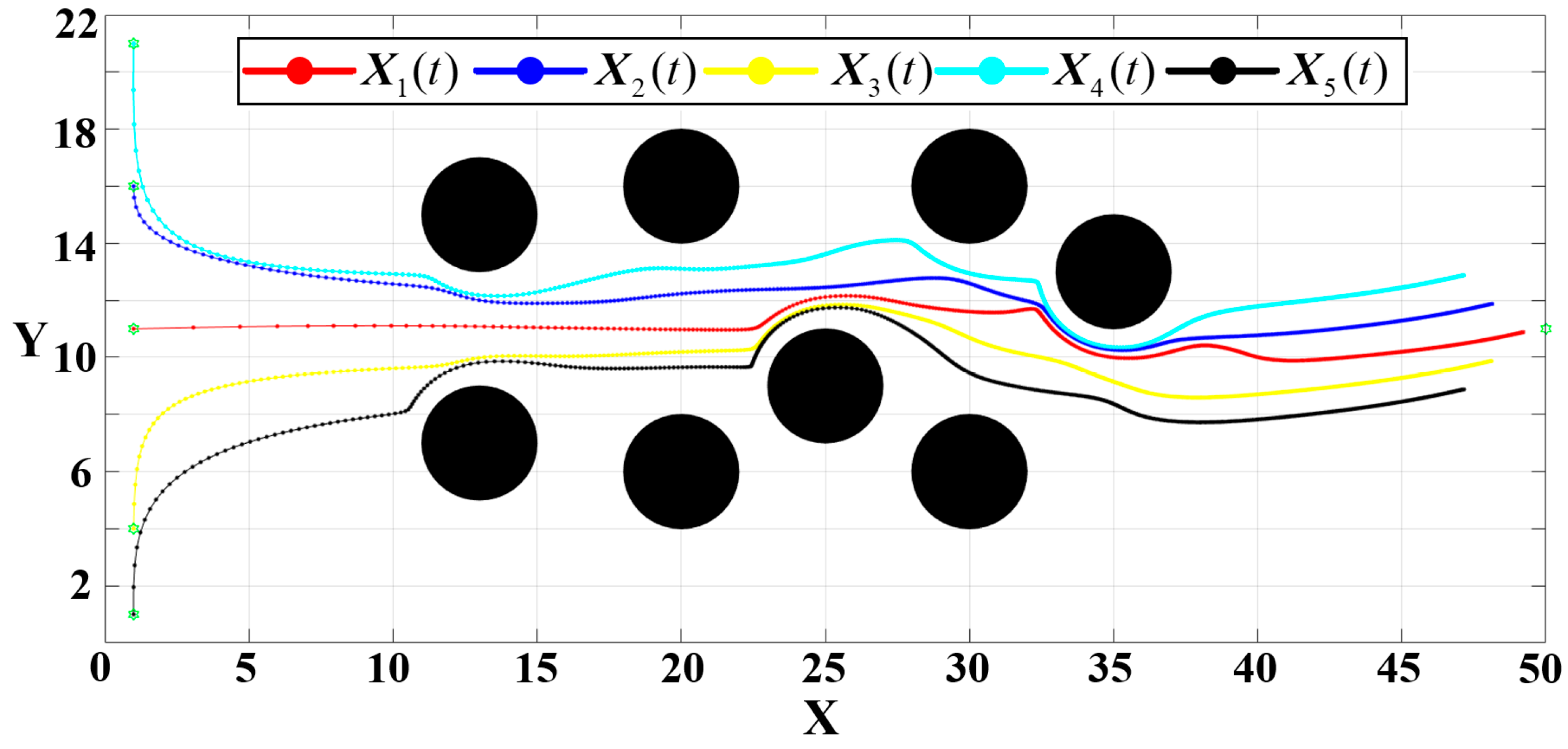
To evaluate the performance of the proposed algorithm in environments populated with multiple obstacles, a set of complex scenarios is designed. The attractive gain $k_{atti}$, the initial positions of the five UAVs, the target point for the leader, the obstacle radius, and the influence radius are all kept consistent with the previous experiments. The specific configuration is set as $k_{att0}=3$ and $k_{rep}=3$.

The formation trajectory in this complex obstacle environment is illustrated in Figure 24, where each dot represents a discrete position of the UAV at a given timestep. The density of these path points serves as an indicator of the UAV’s velocity—denser points signify slower movement. The adaptive attractive gain function $k_{atti}$ defined in Equation (18) effectively modulates the UAV’s velocity throughout the trajectory. The UAVs accelerates when outside obstacle influence zones, decelerates upon entering obstacle-affected regions, and then accelerates again after bypassing the obstacles. Finally, as the UAVs approach the convergence radius ${\rho }_g$ around the target point, they decelerate to ensure precise arrival.

The evolution of errors in both the $x$ and $y$ directions is presented in Figure 25.

As shown in Figure 25, the formation completes the entire avoidance and convergence process in just 0.131 $s$. The final deviation from the target is 0.00251 in the $x$ direction and −0.00768 in the $y$ direction, respectively. These results demonstrate that the proposed algorithm enables the multi-UAV formation to navigate efficiently and accurately, even under complex multi-obstacle conditions.

To demonstrate the improvement of the fast convergence control rate, adaptive gravitational gain and resultant force optimizing the momentum smoothing proposed in this paper on the traditional APF-F, under the conditions of the obstacle avoidance experiment in the complex environment in this subsection, we conducted the ablation experiment in Appendix A.

4.4. Test of Escaping Semi-Enclosed Obstacles

This subsection evaluates the formation’s ability to escape from semi-enclosed obstacle regions—a common cause of local minima in traditional potential field methods. The attractive gain parameters are set as follows: $h_1=40$, $h_2=h_3=h_4=h_5=4$, ${\tau }_2={\tau }_3={\tau }_4={\tau }_5=4$, ${\rho }_g=0.2$, $k_{att0}=3$ and $k_{rep}=3$.

The initial positions of the five UAVs are defined as ${\mathit{X}}_1(0)={(1,2)}^T$, ${\mathit{X}}_2(0)={(0,7)}^T$, ${\mathit{X}}_3(0)={(0,5)}^T$${\mathit{X}}_4(0)={(0,7)}^T$, and ${\mathit{X}}_5(0)={(0,5)}^T$, with the leader’s target point set as ${\mathit{X}}_{g1}={(13,12)}^T$. The circular obstacle is defined with a radius of 0.5 and an influence range ${\rho }_0=3$.

The simulated annealing parameters are defined as follows: initial temperature $T_0=10$, attenuation coefficient $\beta =0.99$, rotation constant $c=1.28$ and escape angle threshold ${\theta }_0={\displaystyle \frac{4}{9}}\pi$.

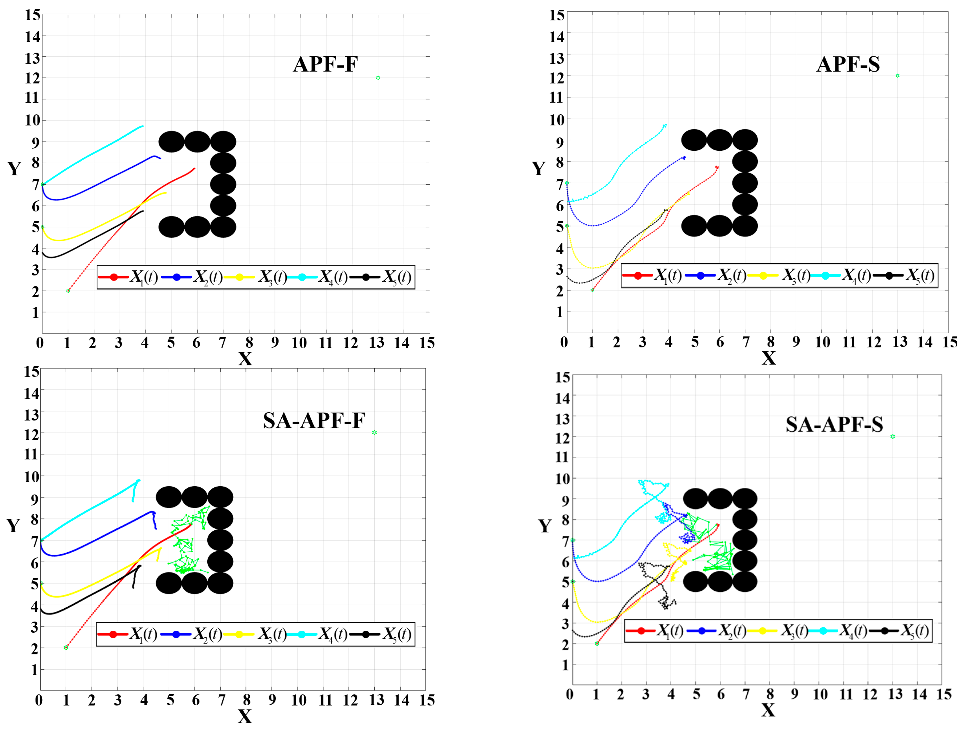
In the first test, the obstacle is modeled as a left-open semi-enclosed structure. The escape trajectory of the UAV formation is illustrated in Figure 26.

As shown in Figure 26, the green trajectory denotes the path of the leader (UAV 1) as it successfully escapes the semi-enclosed obstacle using the improved deflected simulated annealing mechanism. The escape path is short and efficient, with the total process completed in 0.355 $s$.

The left-open semi-enclosed obstacle escape test is conducted using the traditional algorithms APF-F and APF-S, and SA-APF-F and SA-APF-S, with the addition of the traditional SA algorithm on their basis. The simulated path map is shown in Figure 27.

From Figure 27, APF-F and APF-S are completely incapable of escaping from the local minima. SA-APF-F and SA-APF-S are also almost unable to escape when facing local minima situations such as semi-enclosed obstacles. They randomly collide within the obstacles along very chaotic paths and disrupt the entire formation. It is indicated that none of these methods are applicable to the escape of multiple UAV formations from semi-enclosed obstacles.

To test the stability of the algorithm, we conducted a sensitivity analysis with a 10% change in the main control parameters, including $h_i$ and ${\tau }_i$ in Equation (18) and rotation constant $c$, to observe the change in the escape success rate. The results are shown in

Table 5. The variation of the success rate with the change in the main parameters.

Parameter	−5%	−3%	0	3%	5%
$h_i$	96%	96%	96%	96%	95%
${\tau }_i$	96%	96%	96%	96%	96%
$c$	95%	96%	96%	94%	90%

as follows.

From Table 5, making small-scale changes to the main parameters has almost no impact on the success rate.

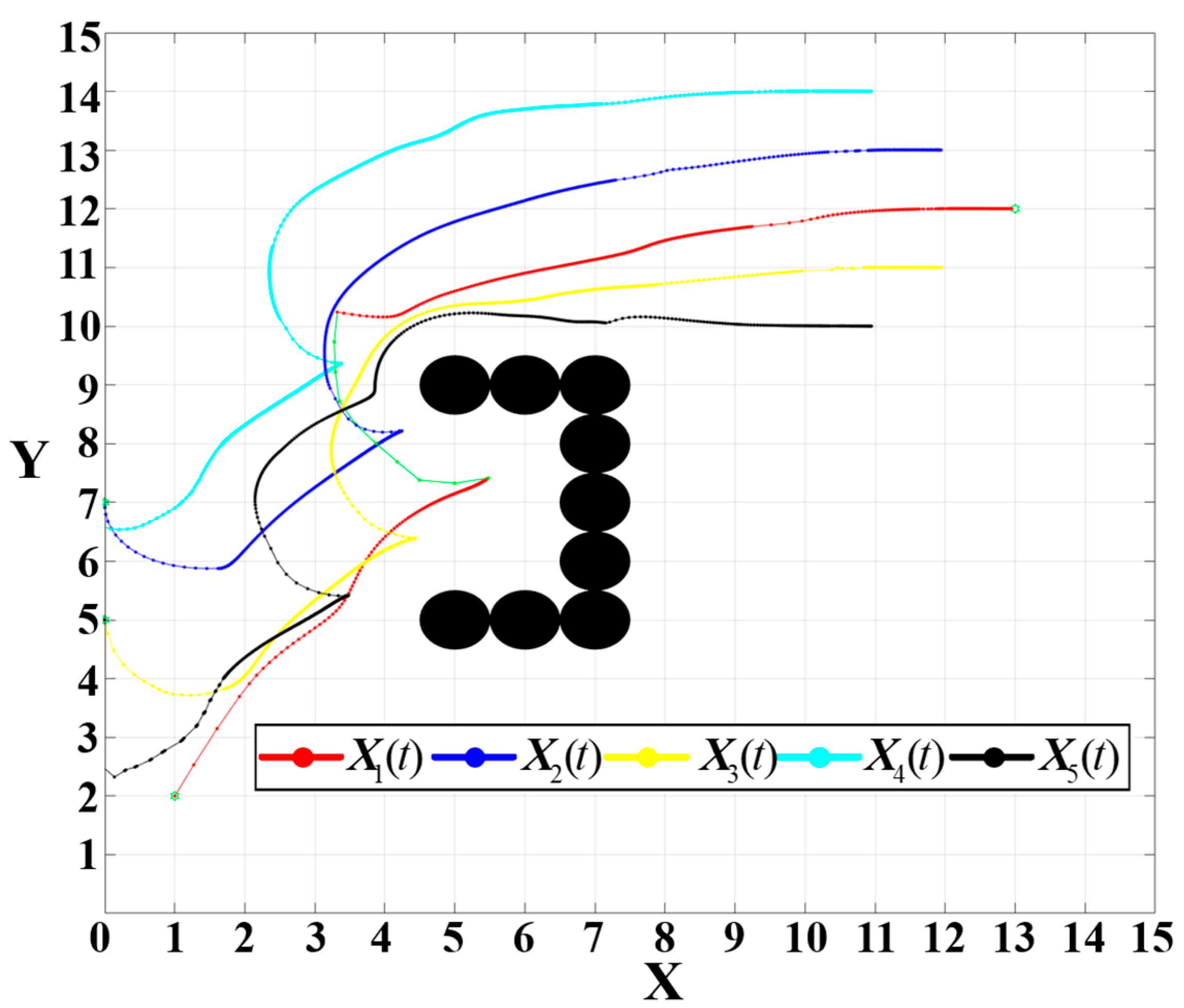
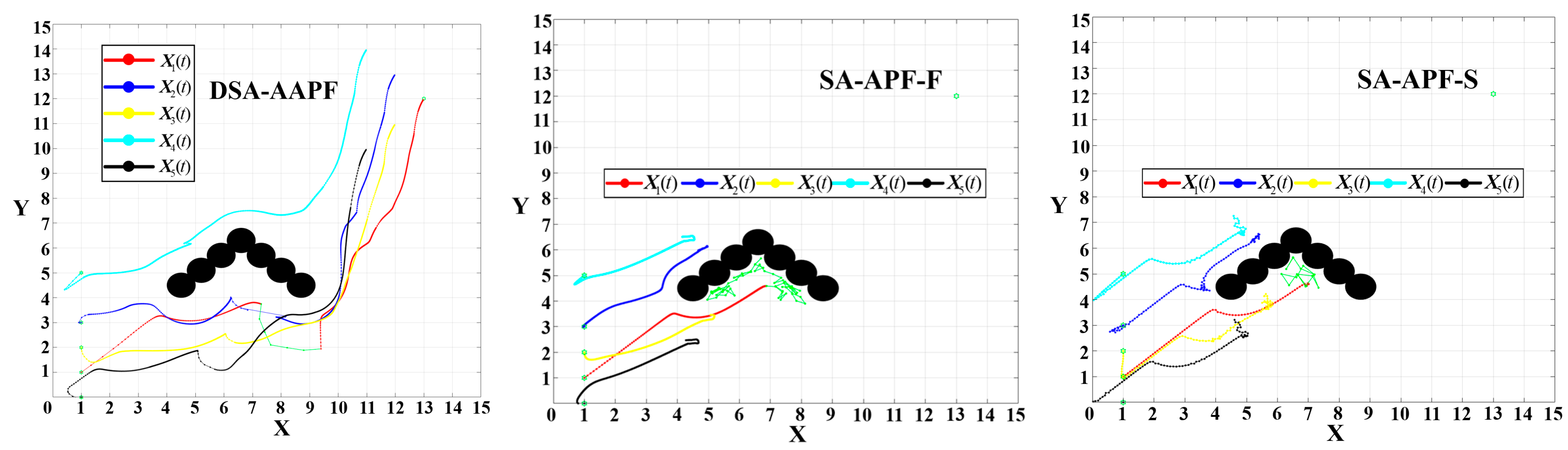
In the second test, the obstacle is configured as a bottom-open semi-enclosed structure. The initial positions of the UAVs remain unchanged. The final escape angle threshold is maintained at ${\theta }_0={\displaystyle \frac{2}{5}}\pi$ and all the other parameters are identical to those used in the previous test. The initial positions of the five UAVs are defined as ${\mathit{X}}_1(0)={(1,1)}^T$, ${\mathit{X}}_2(0)={(1,3)}^T$, ${\mathit{X}}_3(0)={(1,2)}^T$, ${\mathit{X}}_4(0)={(1,2)}^T$, and ${\mathit{X}}_5(0)={(1,0)}^T$. A comparative experiment is conducted between DSA-AAPF and SA-APF-F and SA-APF-S.

The escape trajectory for this configuration is depicted in Figure 28.

From Figure 28, obviously, in the DSA-AAPF algorithm, the navigator successfully avoids the semi-closed obstacles that are open at the bottom and completes this process with a short and efficient path. The total execution time is 0.466 $s$. The SA-APF-F and SA-APF-S algorithms still can hardly escape from the semi-enclosed obstacles with open bottoms, and the paths they attempt to escape via are very chaotic.

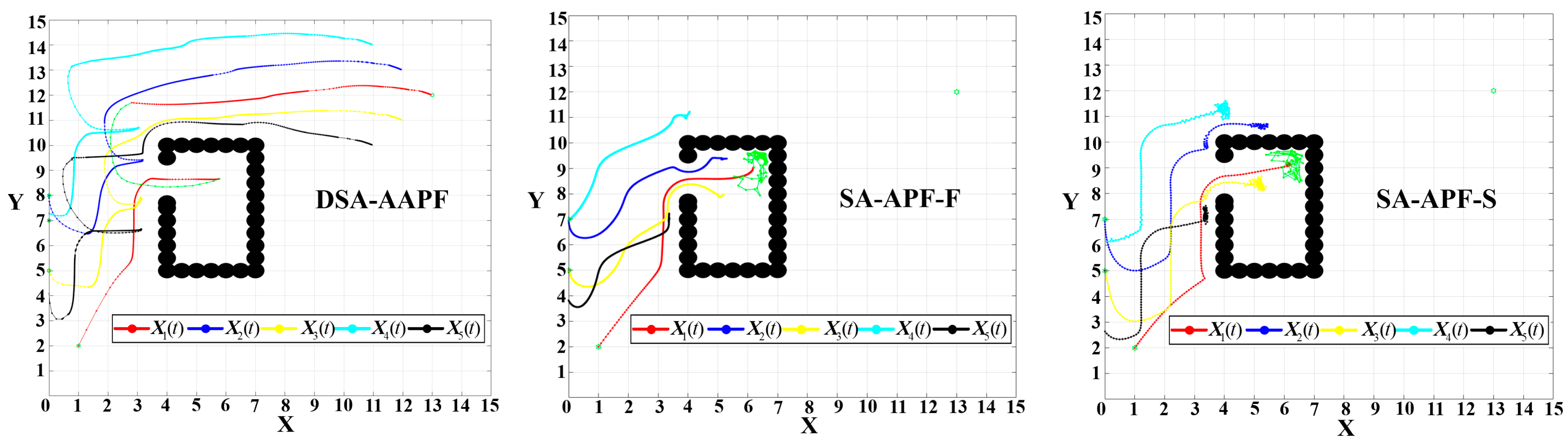
In the third experiment, the obstacle is expanded to leave only a small gap to verify the escape ability of DSA-AAPF in more complex situations, and comparative experiments are conducted simultaneously with SA-APF-F and SA-APF-S. The rotation constant $c=1.165$. The simulation path diagrams in the three cases are shown in Figure 29.

From Figure 29, the DSA-AAPF algorithm still allows the navigator to escape nearly fully enclosed obstacles via a shorter path, and the other two algorithms still cannot.

After a large number of experiments, we can draw the conclusions in

Table 6. The success rate comparison of DSA-AAPF, APF-F, APF-S, SA-APF-F and SA-APF-S when escaping from the local minima caused by various obstacles.

Algorithm	Left-Open Semi-Enclosed Obstacle	Bottom-Open Semi-Enclosed Obstacle	Nearly Fully Enclosed Obstacle
DSA-AAPF	96%	98%	92%
APF-F	Failure	Failure	Failure
APF-S	Failure	Failure	Failure
SA-APF-F	Extremely low probability	Extremely low probability	Failure
SA-APF-S	Extremely low probability	Extremely low probability	Failure

. DSA-AAPF has an extremely high success rate when encountering the above three obstacles, while APF-F and APF-S have no ability to escape the local minima. SA-APF-F and SA-APF-S have an extremely low probability of escape only when encountering local minima caused by relatively simple obstacles. They are ineffective when encountering complex obstacles, and the paths for attempting to escape the obstacles are very chaotic, making them not suitable for multi-UAV formations. To sum up, it is sufficient to prove that DSA-AAPF has higher superiority and robustness compared with several other traditional algorithms.

5. Conclusions

This paper proposes an enhanced deflected simulated annealing–adaptive artificial potential field (DSA-AAPF) algorithm to address the limitations inherent in traditional artificial potential field (APF) methods. The improved framework redefines the potential field functions and integrates the APF with a leader–follower distributed control strategy for multi-UAV formation tasks. To mitigate the oscillations caused by excessive velocity when the UAVs are far from the target and approach obstacles abruptly, a modified force computation model is introduced. This change retains a fraction of the previous timestep’s resultant force, thereby ensuring smoother UAV trajectories. To address the challenge of an inadequate attractive force near the target—leading to failure in terms of convergence—a novel adaptive attractive gain function is designed. This allows the UAVs to dynamically adjust their movement speed based on the proximity to obstacles and the goal, and it is supported by a controller with fast convergence characteristics, ensuring that the formation reaches the target both accurately and efficiently. Furthermore, to overcome the local minima problem typically caused by semi-enclosed obstacles, the simulated annealing algorithm is refined. The proposed method enables UAVs to escape these traps by applying a continuous deflection force that guides the UAV along an arc-like path. Comprehensive simulation experiments—including an oscillation test, formation reconfiguration, obstacle avoidance in cluttered environments, and escape from semi-enclosed obstacles—demonstrated the efficacy and robustness of the DSA-AAPF algorithm.

Three promising directions are identified for future research.

(1) Extension to 3D dynamic environments

The current study focuses solely on two-dimensional environments with static circular obstacles. A natural progression would involve extending the algorithm to operate in three-dimensional spaces, accounting for dynamic and irregularly shaped obstacles to enhance the real-world applicability. This extension requires integrating 3D kinematic models, such as Dubins paths or spline-based trajectories, to handle the UAV pitch and yaw dynamics, while incorporating velocity obstacles or reinforcement learning for dynamic collision avoidance. Additionally, signed distance fields (SDFs) or voxel grids could efficiently represent complex geometries, although the computational overhead remains a key challenge for real-time processing.

(2) Path optimization in semi-enclosed regions

While the improved deflected simulated annealing method effectively enables UAVs to escape from semi-enclosed obstacles, further investigation is warranted to identify the optimal escape trajectories that minimize the energy consumption and execution time. A hybrid optimization approach, combining gradient-based methods like sequential quadratic programming with metaheuristics, could refine the escape paths for efficiency. Additionally, formulating a multi-objective optimization problem that balances the energy expenditure (e.g., drag-induced losses) against the time delays would enhance the practicality, while topological tools such as homology analysis could help identify structurally optimal escape routes in cluttered environments.

(3) Real UAV swarm limitations

In this paper, Equation (1) simplifies the dynamic model of the UAV. It is necessary to further extend the algorithm to the three-dimensional space to use the six-degree-of-freedom dynamic model of the UAV, accounting for realistic aerodynamics and control surfaces. Furthermore, in real UAV swarms, the communication delays, packet losses, and limited energy budgets critically impact the formation control and collision avoidance. Future work should embed robust communication protocols, such as delay-tolerant networking (DTN) or consensus algorithms under intermittent connectivity, while integrating energy-aware path planning to extend the operational endurance under battery constraints. These considerations are essential for deploying the algorithm in real-world scenarios where imperfect communication and finite energy resources dominate the system performance.