Long-Duration UAV Localization Across Day and Night by Fusing Dual-Vision Geo-Registration with Inertial Measurements

Abstract

Remote sensing visual-light spectral (VIS) maps provide stable and rich features for geo-localization. However, it still remains a challenge to make use of VIS map features as localization references at night. To construct a cross-day-and-night localization system for long-duration UAVs, this study proposes a visual–inertial integrated localization system, where the visual component can register both RGB and infrared camera images in one unified VIS map. To deal with the large differences between visible and thermal images, we inspected various visual features and utilized a pre-trained network for cross-domain feature extraction and matching. To obtain an accurate position from visual geo-localization, we demonstrate a localization error compensation algorithm with considerations about the camera attitude, flight height, and terrain height. Finally, the inertial and dual-vision information is fused with a State Transformation Extended Kalman Filter (ST-EKF) to generate long-term, drift-free localization performance. Finally, we conducted actual long-duration flight experiments with altitudes ranging from 700 to 2400 m and flight distances longer than 344.6 km. The experimental results demonstrate that the proposed method’s localization error is less than 50 m in its RMSE.

1. Introduction

Long-endurance UAVs are characterized by long durations, long flight distances, and high altitudes. Therefore, long-endurance UAVs require navigation systems to maintain robust and accurate localization performance for long periods. The primary navigation method used on current long-endurance UAVs is GNSS–inertial integrated systems. However, GNSS is susceptible to interference, leading to task failure or catastrophes in challenging environments.

As an emerging navigation technology, visual navigation is fully autonomous and resistant to interference, making it an alternative method to GNSS. The visual navigation used can be broadly divided into two categories: the Relative Visual Localization (RVL) methods and the Absolute Visual Localization (AVL) methods [1]. RVL uses image flows to estimate the relative motion, such as Visual Odometry (VO) [2,3,4] and Visual Simultaneous Localization and Mapping (VSLAM) [2,5,6], while the AVL compares camera images with a reference map to determine the carrier’s absolute position.

As most long-duration UAVs are equipped with navigation-level inertial systems for accurate dead reckoning, this work focuses on using AVL techniques to compensate for the inertial drifts and achieve cross-day-and-night accurate localization.

In AVL methods, template matching and feature matching are two common approaches for matching aerial images with reference maps [1]. In order to achieve better matching results, obtaining a top-down view similar to the reference map is necessary. However, in UAV application scenarios, due to the horizontal attitude changes in the UAV, the camera axis is typically not perpendicular to the ground. Although mechanisms such as gimbals and stabilizers have been used to maintain the camera’s perpendicularity to the ground [7,8,9,10], the limitations in UAV size make it difficult to accommodate these mechanical structures with multiple sensors in different positions on the UAV.

Long-range UAVs need to take long flights; therefore, the vision geo-registration method needs to face the scene of night work. However, most of the traditional AVL research focuses on visible-light image matching. At nighttime, visible-light-image-based AVL methods usually cannot work well. Using thermal images instead is a realizable way to settle it. AVL methods also need reference maps, but few institutions devote themselves to building complete high-precision infrared radiation (IR) maps. Multimodal image matching (MMIM) is an interesting research topic in image matching, which is studied widely in the medical field [11]. Matching IR and visible images (IR-VIS) is one of the most important research directions in MMIM. Similar to the conventional visible image-matching methods, the IR-VIS method also can be divided into template matching [12,13] and feature matching [14,15,16,17]. Learning-based methods [18,19] are also used in complex scenes that cannot extract descriptors directly. However, most MMIM methods only focus on street scenes and structured scene image registration.

We propose a long-term localization method by fusing the inertial navigation and cross-domain visual geo-registration component, as shown in Figure 1. This method includes three main components: inertial navigation, visible/thermal vision-based geo-localization, and inertial–visual integrated navigation. Compared to traditional matching localization algorithms, our research aims at the day-and-night visual localization needs under long-term localization conditions. Therefore, we propose using deep learning features to describe and match images using graph neural networks. In addition, we analyze the potential errors in visual matching localization and propose compensation methods. The main contributions of our work are as follows:

• To match visible and thermal camera images to a remote sensing RGB map, we investigate several visual features and propose outlier filtering methods to achieve cross-day-and-night geo-registration performance.
• To obtain accurate localization results from geo-registration, we analyze the influence of horizontal attitude on the visual geo-localization, and we propose a compensation method to correct the localization from raw image registration.
• We conduct actual long-duration flight experiments in different situations. The experiments include visual registration using various feature-extracting methods on visible light and thermal images, geo-localization with attitude compensation, and integrated navigation. The experimental results prove the effectiveness of our methods.

This paper is organized as follows. Section 2 presents the research related to our work. Section 3 introduces the proposed method, including our integrated navigation framework, cross-domain visual registration method, geo-localization method, and filter state updating. Section 4 describes our experiments, including system setup, dataset description, data evaluation criteria, and experiment results. Section 5 presents our conclusion.

2. Related Works

We focus on integrating dual-vision geo-registration and inertial measurement units (IMUs) across day and night. Therefore, we focus on two related categories of work: visual navigation methods and IR-VIS methods.

2.1. Visual Navigation

Traditional visual navigation technologies can be divided into RVL and AVL [1]. VO and VSLAM are the two leading technologies under RVL, with VO often serving as a component of VSLAM. Classic pure visual relative localization algorithms include SVO [18], DSO [19], and ORB-SLAM [20], among others. Many researchers have concentrated on fusing vision with other sensors to compensate for the integration errors of pure visual relative localization, especially integrating the inertial measurement unit (IMU) with vision systems. Representative works include VINS-mono [4] and ORB-SLAM3 [5]. In recent years, RVL based on non-visible-light images has also been applied in navigation [21]. RVL can estimate the relative position of the carrier, but without prior geographical coordinates, RVL cannot determine the carrier’s absolute position in the geographical coordinate system. Moreover, VO has cumulative errors, and VSLAM requires loop closure to achieve high-precision localization and mapping, which limits the application of RVL technology in UAVs, especially for long-term and large-scale navigation requirements.

AVL aims to match camera images with reference maps to determine the carrier’s position on the map. When the reference map can be aligned with the geographical coordinate system, the absolute position of the carrier in the geographical coordinate system can be determined. Image matching methods are mainly divided into template matching and feature matching. Template matching involves treating aerial images as part of the reference map, so the prerequisite is to transform them into images with the same scale and direction as the reference map before comparing them. The main parameters used include Normalized Cross-Correlation (NCC) [9,22], Mutual Information (MI) [23], and Normalized Information Distance (NID) [8]. Though template matching methods achieve higher localization precision than feature-based methods [24], they need to compare the camera images with the map at the pixel level (raw intensity or normalized intensity); this requires ample space to store the maps and high computation costs to calculate the similarities throughout the maps. At the same time, for better registration between aerial images and reference maps, mechanisms such as gimbals and stabilizers are commonly used to ensure the camera is always perpendicular to the ground [7,8].

Another AVL method is to match features between aerial images and reference maps. Although feature-matching methods introduce errors in feature detection and describing steps, it has the advantage that feature-matching methods need less storage and computation cost as they compress raw maps and images to sparse features, which can be efficiently implemented for real-time operation on embedded systems. It is meaningful for real-time processing in airborne equipment. Conte [25] used edge detection to match aerial images with maps, but the results showed a low matching rate. M. Mantelli [10] proposed abBRIEF features based on BRIEF features [26], showing better performance than traditional BRIEF on AVL. J. Surber [27] and others used a self-built 3D map as a reference and matched it with BRISK features [26], also utilizing weak GPS priors to reduce visual aliasing. M. Shan and others [28] constructed an HOG feature query library for the reference map. Since it includes a global search process, this method can determine the carrier’s absolute position without providing prior location information. A. Nassar [29] proposed using SIFT features for image feature description and introduced Convolutional Neural Networks (CNNs) for feature matching and vehicle localization in images.

In summary, while RVL has the disadvantage of cumulative errors, AVL can relatively accurately determine the carrier’s position without relying on prior location information. However, most work directly uses the center point of the matched image in the reference map to approximate the carrier’s position. Incorrect matching and UAV attitudes can significantly affect the results of visual matching localization. Moreover, most works focus on visible-light images, which have poor matching performance at night.

2.2. IR-VIS Method

IR-VIS methods can be classified into template matching and feature matching. In template matching, Yu et al. [13] proposed a strategy to enhance Normalized Mutual Information (NMI) matching. They employed a grayscale weighted window method to extract edge features, thereby reducing the NMI’s joint entropy and local extrema. The author of [12] first transforms the image into an edge map and describes geometrical relations between rough and fine matching by affine and Free-Form Deformation (FFD). The work optimized matching by maximizing the overall similarity of MI between edge maps. As for feature matching, Hrkać, T et al. [14] detected Harris corners from IR and visible images, then used a simple similarity transformation to match them. However, this experiment is performed in situations where images have stable corners. Ma et al. [15] built an inherent feature of the image by extracting the edge map of the image. They propose a Gaussian field criterion to achieve registration. This method shows good performance in registering IR and visible face images. The authors of [16] proposed a scale-invariant Probabilistic Intensity-based Image Feature Detector (PIIFD) for corner feature description. In addition, an affine matrix estimation method based on the Bayesian framework is proposed. The authors of [17] first extracted the edge using the morphological gradient method. They used a C_SIFT detector on the edge map to search for distinct points and used BRIEF for description, finally making scale- and orientation-invariant matching come true.

With the development of deep learning, matching methods based on learning have become essential in IR-VIS research. The authors of [30] proposed a two-phase Graph Neural Network (GNN), which includes a domain transfer network and a geometrical transformer module. This method was used to obtain better-warped images across different modalities. Baruch et al. [31] used a hybrid CNN framework to extract and match features jointly. The framework consists of a Siamese CNN and a dual non-weight-sharing CNN, which can capture multimodal image features.

We can see that although many methods are proposed for use in IR-VIS, most focus on the image registration of structured scenes, like cities, buildings, and streets. Additionally, some research focuses on facial images. Utilizing the IR-VIS method to achieve vision geo-registration has rarely been researched. Distinguishing from structured scenes and human faces, geo-registration problems focus on unstructured scenes represented by the natural environment. Particularly for some situations, like forest, desert, gobi, and ocean, a few features present an excellent challenge for matching.

3. Method

This section presents our visual–inertial navigation system (VINS) framework, which comprises three components: inertial navigation, vision geo-registration, and integrated navigation. The vision geo-registration component matches camera images (including both visible-light and thermal images) to the reference map and calculates the geolocation of the UAV. The INS component provides high-frequency navigation state and covariance (including attitude, velocity, and position) prediction. The integrated navigation component utilizes vision geo-registration results to compensate for the drift caused by INS prediction. The framework is illustrated in Figure 2.

3.1. Visual–Inertial System State Construction and Propagation

In this part, we present the filter used in the integrated navigation, which includes state construction, nominal state propagation, and covariance propagation. We use the State Transformation Extended Kalman Filter (ST-EKF) [32,33] to estimate the navigation state.

3.1.1. Nominal State Propagation

Following Ref. [33], we define the nominal state vector $\mathit{x}$ as follows:

$$\mathit{x}={\left[\begin{array}{ccc}\mathit{q}& \mathit{v}& \mathit{p}\end{array}\right]}^T$$

(1)

where $\mathit{q}$, $\mathit{v}$ and $\mathit{p}$ are attitude, velocity, and position, respectively.

$\mathit{q}$, $\mathit{v}$ and $\mathit{p}$ need to be calculated using IMU data. Unlike most visual/inertial navigation systems based on Micro-Electromechanical System IMUs (MEMS IMUs) [4,5,6], which apply numerical integration on the state differential equations, we used optimal INS algorithms with coning and sculling corrections [34,35,36,37], as long-duration vehicles are usually equipped with navigation-grade IMUs.

3.1.2. Filter State

The same as Ref. [33], the error states $\delta \mathit{x}$ can be expressed as:

$$\delta \mathit{x}={\left[\begin{array}{ccccc}\delta \mathit{\varphi }& \delta \mathit{v}& \delta \mathit{r}& {\mathit{b}}_g& {\mathit{b}}_a\end{array}\right]}^T$$

(2)

where $\delta \mathit{\varphi }$, $\delta \mathit{v}$ and $\delta \mathit{r}$ are attitude error, velocity error, and position error, respectively. ${\mathit{b}}_g$ and ${\mathit{b}}_a$ are biases of gyros and accelerometers, respectively.

To achieve consistent state estimation results, we employ the ST-EKF model to express the kinematics of error states in the North-East-Down (NED) frame as:

$$\begin{array}{cc}\delta {\dot{\mathit{\varphi }}}^n=& -{\mathit{\omega }}_{in}^n\wedge \delta {\mathit{\varphi }}^n+\delta {\mathit{\omega }}_{in}^n-{\mathit{C}}_b^n\cdot \delta {\mathit{\omega }}_{ib}^b\\ \delta {\dot{\mathit{v}}}_{\mathit{\varphi }}^n=& -\left[{\mathit{g}}^n\wedge +\left({\tilde{\mathit{v}}}_{eb}^n\wedge \right)\left({\mathit{\omega }}_{ie}^n\wedge \right)\right]\delta {\mathit{\varphi }}^n-\left(2{\mathit{\omega }}_{ie}^n+{\mathit{\omega }}_{en}^n\right)\wedge \delta {\mathit{v}}_{\mathit{\varphi }}^n\\ & +{\mathit{C}}_b^n\left({\mathit{b}}_a+{\mathit{w}}_a\right)+\left({\tilde{\mathit{v}}}_{eb}^n\wedge \right){\mathit{C}}_b^n\left({\mathit{b}}_g+{\mathit{w}}_g\right)+{\mathit{v}}_{eb}^n\wedge \delta {\mathit{\omega }}_{ie}^n\\ \delta {\dot{\mathit{r}}}^n=& {\mathit{F}}_{rr}\left({\tilde{\mathit{v}}}_{eb}^n\wedge \right)\delta {\mathit{\varphi }}^n+{\mathit{F}}_{rv}\cdot \delta {\mathit{v}}_{\mathit{\varphi }}^n+{\mathit{F}}_{rr}\cdot \delta {\mathit{r}}_{\mathit{\varphi }}^n\end{array}$$

(3)

where ${\mathit{\omega }}_{ie}^n$ is the earth rotation vector; ${\mathit{\omega }}_{ie}^n+{\mathit{\omega }}_{en}^n={\mathit{\omega }}_{in}^n$ is the angular rate vector of the navigation frame relative to the inertial frame; ${\tilde{\mathit{v}}}_{eb}^n$ is the estimated value of velocity; $\delta {\mathit{\varphi }}^n$ is the attitude error vector in the navigation frame; ${\mathit{C}}_b^n$ is the direction cosine matrix (DCM) from body frame to navigation frame; ${\mathit{g}}^n$ is the gravity vector; ${\mathit{w}}_a$ and ${\mathit{w}}_g$ are the white noises of the gyros and accelerometers, respectively, and $\delta {\mathit{\omega }}_{ib}^b={\mathit{b}}_g+{\mathit{w}}_g$; and the symbol $\wedge$ represents the transformation from vectors to skew-symmetric matrices. ${\mathit{F}}_{rr}$ and ${\mathit{F}}_{rv}$ can be expressed as follows:

$${\mathit{F}}_{rr}=\left[\begin{array}{ccc}0& 0& -{\displaystyle \frac{v_N}{{\left(R_N+h\right)}^2}}\\ {\displaystyle \frac{v_E\tan L}{\left(R_E+h\right)\cos L}}& 0& -{\displaystyle \frac{v_E}{{\left(R_E+h\right)}^2}}\\ 0& 0& 0\end{array}\right]\begin{array}{cc}& \end{array}{\mathit{F}}_{rv}=\left[\begin{array}{ccc}{\displaystyle \frac{1}{R_N+h}}& 0& 0\\ 0& {\displaystyle \frac{1}{\left(R_E+h\right)\cos L}}& 0\\ 0& 0& -1\end{array}\right]$$

(4)

where $v_N$ and $v_E$ are northward and eastward velocity, respectively. $R_N$ and $R_E$ are the radius of curvature in meridian and prime vertical, respectively. $L$ is the latitude, and $h$ is the height.

Note that, compared with the common kinematics of error states, the specific force in the velocity error differential equation is replaced by the gravity vector, which helps to improve the state estimation accuracy and consistency in dynamic conditions [32,33].

According to Equations (3) and (4), the error model of INS at time $t$ can be described as follows:

$$\delta \dot{\mathit{x}}\left(t\right)=\mathit{F}\left(t\right)\delta \mathit{x}\left(t\right)+\mathit{G}\left(t\right)\mathit{u}\left(t\right)$$

(5)

where $\mathit{F}$ is the system matrix, $\mathit{G}$ is the noise input matrix, and $\mathit{u}$ is the noise vector of the system. They are the same as those in the traditional Extended Kalman Filter (EKF) of integrated navigation.

3.1.3. Covariance Propagation

From the vision geo-registration that will be presented in Section 3.2 and INS prediction presented in Section 3.1.1, we obtain a 2D visual localization position $\left[\begin{array}{cc}lat{i}_V& long{i}_V\end{array}\right]$ and an INS prediction position $\left[\begin{array}{cc}lat{i}_{INS}& long{i}_{INS}\end{array}\right]$. We define the observation vector $\mathit{z}={\left[\begin{array}{cc}{\mathit{z}}_{lati}& {\mathit{z}}_{longi}\end{array}\right]}^T={\left[\begin{array}{cc}lat{i}_V-lat{i}_{INS}& long{i}_V-long{i}_{INS}\end{array}\right]}^T$. Then, the observation equation can be described as:

$$\mathit{z}=\left[\begin{array}{ccc}{0}_{2\times 6}& {\mathit{I}}_{2\times 2}& 0_{2\times 7}\end{array}\right]\delta \mathit{x}$$

(6)

The subscript above represents the dimensions of the matrix.

Then, the observation matrix $\mathit{H}$ can be given as:

$$\mathit{H}=\left[\begin{array}{ccc}{0}_{2\times 6}& {\mathit{I}}_{2\times 2}& 0_{2\times 7}\end{array}\right]$$

(7)

In the covariance propagation, we need to predict the covariance matrix ${\mathit{P}}_{k|k-1}$ first as follows:

$${\mathit{P}}_{k|k-1}={\mathit{\Phi }}_{k,k-1}{\mathit{P}}_{k-1}{\mathit{\Phi }}_{k,k-1}^T+{\mathit{Q}}_{k-1}$$

(8)

where ${\mathit{\Phi }}_{k,k-1}$ is the discretized system matrix, and ${\mathit{Q}}_{k-1}$ is the noise distribution covariance matrix.

Then, we calculate the Kalman gain ${\mathit{K}}_k$ as:

$${\mathit{K}}_k={\mathit{P}}_{k|k-1}{\mathit{H}}^T{\left(\mathit{H}{\mathit{P}}_{k|k-1}{\mathit{H}}^T+{\mathit{R}}_k\right)}^{-1}$$

(9)

where ${\mathit{R}}_k$ is the measurement noise covariance matrix of the sensors.

Finally, we update the covariance matrix:

$${\mathit{P}}_{k|k}=\left(\mathit{I}-{\mathit{K}}_k\mathit{H}\right){\mathit{P}}_{k|k-1}{\left(\mathit{I}-{\mathit{K}}_k\mathit{H}\right)}^T+{\mathit{K}}_k{\mathit{R}}_k{\mathit{K}}_k^T$$

(10)

The diagonals of the updated covariance matrix contain elements related to the horizontal position $\left[\begin{array}{cc}{p}_{k-lati}& p_{k-longi}\end{array}\right]$, which will be used to construct the Gaussian elliptic constraint in integrated navigation.

3.2. Cross-Domain Visual Registration

Our work mainly aims at long-duration navigation, which means that visual geo-localization needs to remain effective at nighttime. This section will present the method for achieving cross-domain visual registration.

3.2.1. Feature Extraction and Matching Method

To achieve day–night vision-based localization, the key is to develop visual features effective in visible-light and thermal images. Although a series of hand-crafted features and learned features have been used in RGB-image geo-registration [7,8,9,10], few works have shown the capabilities in thermal images.

To obtain a unified feature for cross-domain image matching, we investigated multiple hand-crafted and learned features, including SIFT [38], XFeat [39], and SuperPoint [40]. Figure 3 shows some samples of the performance of these features on visible-light and thermal images. SIFT applies to visible-light images but demonstrates limited effectiveness on thermal images. XFeat can also be used comparably to SuperPoint in visible and thermal images, but XFeat exhibits fewer matching points and a lower matching rate than SuperPoint. The investigation shows that SuperPoint shows the best performance in both visible light and thermal matching. In the experimental part, we designed a comparative experiment to prove our conclusion.

3.2.2. Reference Visible Map Pre-Processing

For long-duration navigation, the task areas can be extensive, which can cause difficulties in both storage and real-time processing. Therefore, we need to pre-process the reference map before the task to improve efficiency during the flight.

While the UAVs are equipped with both visible and thermal cameras, we propose only to use remote visible maps for reference, as high-resolution visible maps are easy to obtain.

To improve the algorithm’s efficiency, we divide the map into sub-maps and use the predicted location from INS to load the sub-maps. Figure 4 shows the method for building the reference map set.

Firstly, the remote visible-light map along the planned flight path needs to be pre-downloaded. Then, we separate the whole map into sub-maps with a size of $w_{map}\times h_{map}$. The $w_{map}$ and $h_{map}$ are the actual length of the sub-map in east and north, respectively. When the drone flies to the maximum height in the flight, the sub-map should contain as much of the scenery of the camera image as possible. It means the following:

$$\min (w_{map},h_{map})\ge 2H_{\max }\tan {\displaystyle \frac{\theta }{2}}$$

(11)

where $H_{\max }$ is the maximum height of UAVs, and $\theta$ is the field of view (FOV) of the camera. At the same time, when visual matching localization fails, pure inertial navigation will cause drift. Therefore, it is meaningful to consider appropriately increasing $w_{map}$ and $h_{map}$ to avoid map retrieval failure caused by localization divergence, which, in turn, leads to the complete failure of scene-matching localization. In addition, when the image matching area is close to the edge of the map, matching may fail due to the incomplete matching area. Therefore, when cropping the map, we first crop it to a size of $(w_{map}/2)\times (h_{map}/2)$ and then stitch adjacent $2\times 2$ map blocks into a sub-map. This ensures that there is a 50% overlap between adjacent sub-maps. Finally, we obtain the sub-map image set $\left\{m_{11},m_{12},\dots ,m_{1q},\dots m_{p1},\dots m_{pq}\right\}$ numbered in row and column order.

Then, we build an index of the sub-map set by the latitude and longitude coordinates of the center. Finally, we extract features and descriptors for each sub-map and associate them with the index in

Table 1. Reference map set index.

Sub-Map	Center of Sub-Map (Longitude, Latitude)	Descriptors
$m_{11}$	$(lat{i}_{11},long{i}_{11})$	$(kp{t}_{11}^s,des{c}_{11}^s)$
$m_{12}$	$(lat{i}_{12},long{i}_{12})$	$(kp{t}_{12}^s,des{c}_{12}^s)$
…	…	…
$m_{pq}$	$(lat{i}_{pq},long{i}_{pq})$	$(kp{t}_{pq}^s,des{c}_{pq}^s)$

.

3.2.3. Camera Image Pre-Processing

For long-duration tasks, the UAV can fly at different heights and with various headings, which leads to scale and view variations in the camera images. To reduce the visual aliasing between the camera images and the map, image rotation and scaling are applied before geo-registration. Furthermore, we apply a gamma transformation for thermal images to enhance the contrast, thereby highlighting features more and increasing the number of matching pairs.

• Rotation and Scaling

We perform rotation and scaling pre-processing on the images before feature point extraction to align the geographic coordinate system represented by the images with the reference map (the reference map’s default upward direction being north) and to make the pixel resolution close to that of the reference map. The scaling factor $img\_ratio$ can be given by:

$$\begin{array}{c}img\_rati{o}_x={\displaystyle \frac{H_r}{f_x{\rho }_m}}\\ img\_rati{o}_y={\displaystyle \frac{H_r}{f_y{\rho }_m}}\end{array}$$

(12)

where $H_r$ is relative height, ${\rho }_m$ is the pixel resolution of the sub-map (length in the world coordinate system represented by a single pixel, with units in meters per pixel (m/pix)), $f_x$ and $f_y$ are camera intrinsics, which can be given by Zhang’s camera calibration method [41].

• Thermal Image Gamma Transformation

Infrared imaging is based on the thermal radiation and temperature characteristic differences of ground scenes. However, in high-altitude ground imaging, the collected scenes are mainly large areas of buildings, forests, farmland, roads, etc., with high scene similarity and minor thermal radiation differences, leading to infrared imaging having blurred contours, high noise, and low contrast, which is not conducive to feature extraction. Therefore, before extracting features from infrared images, pre-processing of the infrared images can be performed to extract the potential features of the images better. We choose the gamma transformation to adjust image contrast and brightness to enhance details:

$$s=c{r}^{\gamma },r\in [0,1]$$

(13)

where $r$ is the normalized grayscale value of the infrared image, $c$ is the grayscale scaling factor, $\gamma$ is the gamma value (in this study, we use 0.8 as the gamma value), and $s$ is the normalized grayscale value after gamma transformation.

3.2.4. Camera Map Registration

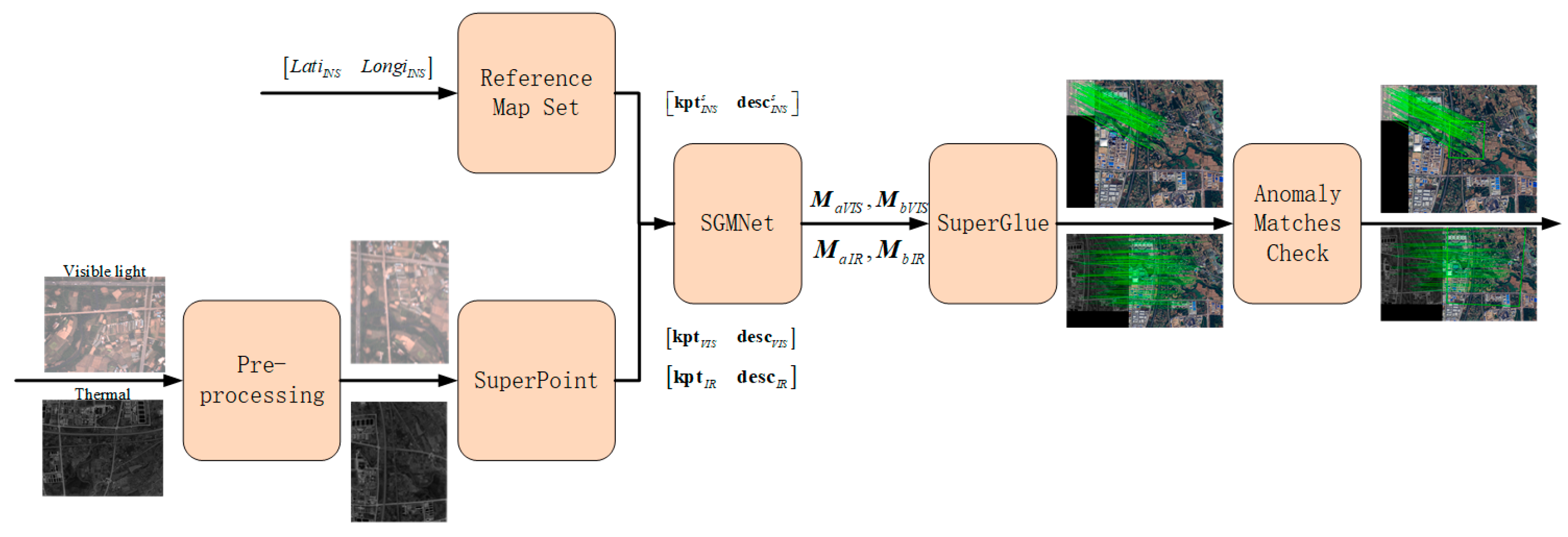
For visual registration, the key lies in matching camera images with reference maps. This section will illustrate the complete process, including sub-map querying, geo-registration method, and anomaly match checking. Figure 5 shows the whole process.

• Sub-map querying

To achieve camera map registration, the first step is to search for the corresponding sub-map. In Section 3.2.2, the sub-maps are indexed by their 2D geo-position. Therefore, we can query the required sub-map features by the position predicted by the INS prediction component.

• Camera map registration method

SuperGlue [42] is a widely used matching method for SuperPoint features. However, the front end of SuperGlue contains multiple attention mechanisms and fully connected networks, which presents a disadvantage for real-time processing. Therefore, we introduce SGMNet [43] to replace this component to improve the efficiency.

When the camera image and sub-map features are sent to the SGMNet, the network first calculates two groups of matches ${\mathit{M}}_a$ and ${\mathit{M}}_b$ as the seed matches. Then, the two seed matches pass through a multi-layer seed graph network to determine the best matches. Finally, the best matches are sent to the back end of SuperGlue to obtain the final matches.

• Anomaly match checking

Due to pre-processing, the matched points of the camera image and sub-map should be connected with lines that are approximately parallel and of similar lengths. Note that, while camera images may be distorted due to pitch and roll, the distortion can be neglected in our method because the application scenario involves medium- to high-altitude operations. Furthermore, the pitch and roll of long-endurance drones during flight are relatively small.

For incorrect matches, the lines are usually not geometrically close, so it is possible to filter out incorrect matched point pairs by using the consistency of the matched point line vectors, thereby removing the inconsistent parts from the set of matched point pairs. Assuming that after matching, there are $n$ pairs of matched points in the collection, where the feature point coordinates in the camera image are $\left[\begin{array}{cc}{u}_i^{img}& v_i^{img}\end{array}\right]$, and the corresponding feature point coordinates on the sub-map are $\left[\begin{array}{cc}{u}_i^{map}& v_i^{map}\end{array}\right]$, then the line vector for each set of matched point pairs is as follows:

$$t_i=\left[\begin{array}{cc}{u}_i^{trans}& v_i^{trans}\end{array}\right]=\left[\begin{array}{cc}{u}_i^{map}-u_i^{img}& v_i^{map}-v_i^{img}\end{array}\right]$$

(14)

For each $t_i$, we can calculate its magnitude $dis{t}_i$ and slope $slop{e}_i$:

$$\begin{array}{c}dis{t}_i=\sqrt{{(u_i^{trans})}^2+{(v_i^{trans})}^2}\\ slop{e}_i={\displaystyle \frac{v_i^{trans}}{u_i^{trans}}}\end{array}$$

(15)

We define the distance consistency threshold $\sigma$ and direction consistency threshold $\omega$; then, we can obtain the consistency set $si{m}_i$ for each $t_i$:

$$\begin{array}{c}si{m}_i=\left\{t_j|dis{t}_i-dis{t}_j\le \sigma ,\arctan (slop{e}_i)-\arctan (slop{e}_j)\le \omega \right\}\\ i,j=1,2,\dots ,n\end{array}$$

(16)

$si{m}_i$ represents the set of matched point pairs, which are similar to the corresponding $t_i$. For each frame, there is a set $si{m}_{\max }$ with the maximum capacity. Then, we consider the matched point pairs in $si{m}_{\max }$ as the filtered matches of the frame. If the number of filtered matches does not meet the threshold of a successful registration, it is considered a failed registration, thereby eliminating incorrectly matched images. If the number of matches meets the threshold, the obtained matches should have eliminated the vast majority of incorrect matches.

3.3. Geo-Localization from Visual Registration

After matching, we obtain a set of matching point pairs. In this section, we illustrate the method for obtaining location from visual registration to achieve the visual geo-localization result. Furthermore, we consider the influence of attitude on geo-localization and the design compensation method.

3.3.1. Geo-Localization

The matching relationship between images can be modeled as an affine transformation. Consequently, in our approach, the geo-location of any point on the reference map within the images taken from UAVs can be determined by computing the affine transformation matrix $\mathit{H}$. We use homography matrix estimation based on Random Sample Consensus (RANSAC) to determine the affine matrix. Note that the roll and pitch of long-endurance UAV are not very large during normal flight. And long-endurance UAVs usually fly at a high altitude. Thus, it can be assumed that there is little 3D variation in camera images.

If we assume that the center of the camera image $\left[\begin{array}{cc}{u}_c^{img}& v_c^{img}\end{array}\right]$ is the location of the UAV, we can transform the camera image into the reference map by using $\mathit{H}$. We will obtain the transformed center of the camera image $\left[\begin{array}{cc}{u}_{c-img}^{map}& v_{c-img}^{map}\end{array}\right]$, and the center of the reference map $\left[\begin{array}{cc}{u}_c^{map}& v_c^{map}\end{array}\right]$ represents the location in the real world $\left[\begin{array}{cc}{lati}^{map}& {longi}^{map}\end{array}\right]$. Then, the location of the UAV $\left[\begin{array}{cc}lati& longi\end{array}\right]$ can be given by:

$$\begin{array}{c}lati={lati}^{map}+{\rho }_m(u_{c-img}^{map}-u_c^{map})\\ longi={longi}^{map}+{\rho }_m(v_{c-img}^{map}-v_c^{map})\end{array}$$

(17)

3.3.2. Attitude Error Compensation

In this part, we use the NED (north-east-down) local geodetic coordinate frame as the navigation coordinate frame (n-frame) and the FRD (front-right-down) frame as the carrier coordinate frame (b-frame). Then, we can define rotation matrices:

We can define a unit vector $e_b={\left[\begin{array}{ccc}0& 0& 1\end{array}\right]}^T$ in the n-system. Note that the subscripts “$b$” and “$n$” represent the vectors in the corresponding frames.

Then, we can transform the vector to the body frame as:

$$\begin{array}{cc}{e}_n& =\left[\begin{array}{ccc}\cos \phi & -\sin \phi & 0\\ \sin \phi & \cos \phi & 0\\ 0& 0& 1\end{array}\right]\left[\begin{array}{ccc}\cos \theta & 0& \sin \theta \\ 0& 1& 0\\ -\sin \theta & 0& \cos \theta \end{array}\right]\left[\begin{array}{ccc}1& 0& 0\\ 0& \cos \gamma & -\sin \gamma \\ 0& \sin \gamma & \cos \gamma \end{array}\right]e_b\hfill \\ & ={\left[\sin \phi \sin \gamma +\cos \phi \sin \theta \cos \gamma \hspace{1em}\hspace{1em}\sin \phi \sin \theta \cos \gamma -\cos \phi \sin \gamma \hspace{1em}\hspace{1em}\cos \theta \cos \gamma \right]}^T\hfill \end{array}$$

(18)

where $\mathit{r}$, $\theta$ and $\phi$ are roll, pitch, and yaw, respectively.

Then, the eastward error $\delta n$ and northward error $\delta e$ can be given by:

$$\begin{array}{c}\delta n=H_r{\displaystyle \frac{\sin \phi \sin \gamma +\cos \phi \sin \theta \cos \gamma }{\cos \theta \cos \gamma }}\\ \delta e=H_r{\displaystyle \frac{\sin \phi \sin \theta \cos \gamma -\cos \phi \sin \gamma }{\cos \theta \cos \gamma }}\end{array}$$

(19)

where $H_r$ is the relative height of the UAV. And Figure 6 shows the error caused by attitude.

Note that the error in Equation (19) is in meters within n-frame rather than in latitude and longitude. So, we need to transform the error into latitude and longitude. Then, the visual geo-localization can be described as follows:

$$\left[\begin{array}{c}{lati}_V\\ {longi}_V\end{array}\right]=\left[\begin{array}{c}{lati}_{V-truth}\\ {longi}_{V-truth}\end{array}\right]+\left[\begin{array}{c}{\displaystyle \frac{\sin \phi \sin \gamma +\cos \phi \sin \theta \cos \gamma }{\left(R_N+Alti\right)\cos \theta \cos \gamma }}\\ {\displaystyle \frac{\sin \phi \sin \theta \cos \gamma -\cos \phi \sin \gamma }{\left(R_E+Alti\right)\cos \left(Lati\right)\cos \theta \cos \gamma }}\end{array}\right]H_r$$

(20)

where the positions with subscript “$V$” are the original visual geo-localization position. The positions with subscript “$V-truth$” are the real horizontal position after attitude compensation. $Alti$ is the absolute height of the UAV and $Lati$ is the latitude of the UAV.

After redefining the error, we need to build the new observation equation. The former term is the same as Equation (6). As for the latter term in Equation (20), if we assume that there is little variation with $Alti$, we can regard $Alti$ and $H_r$ as constants. Then, we use Taylor’s Formula and retain the first-order component. Finally, we can obtain the observation equations as Equation (21).

$$\begin{array}{cc}\hfill \mathit{z}& =\left[\begin{array}{cccc}{\mathit{C}}_a& 0_{2\times 3}& {\mathit{I}}_{2\times 2}& 0_{2\times 7}\end{array}\right]\delta \mathit{x}\hfill \\ \hfill {\mathit{C}}_a& =\left[\begin{array}{c}{\mathit{C}}_{lati}^T\\ {\mathit{C}}_{longi}^T\end{array}\right]\hfill \\ \hfill {\mathit{C}}_{lati}& ={\displaystyle \frac{H_r}{R_N+Alti}}\left[\begin{array}{c}{\sec }^2\gamma \sec \theta \sin \phi \\ \tan \gamma \sec \theta \tan \theta \sin \phi +{\sec }^2\theta \cos \phi \\ \tan \gamma \sec \theta \cos \phi -\tan \theta \sin \phi \end{array}\right]\hfill \\ \hfill {\mathit{C}}_{longi}& ={\displaystyle \frac{H_r}{(R_E+Alti)\cos \left(Lati\right)}}\left[\begin{array}{c}-{\sec }^2\gamma \sec \theta \cos \phi \\ {\sec }^2\theta \sin \phi -\tan \gamma \sec \theta \tan \theta \cos \phi \\ \tan \gamma \sec \theta \sin \phi +\tan \theta \cos \phi \end{array}\right]\hfill \end{array}$$

(21)

In Equation (21), we can see that $H_r/R_n+Alti$ and $H_r/(R_e+Alti)\cos \left(Lati\right)$ are usually small in the mid-latitude or low-latitude region, which is usually less than ${10}^{-2}$ of the order of magnitude. In our experiment, it is always less than ${10}^{-5}$. So, ${\mathit{C}}_a$ can be set to $0_{2\times 3}$ directly. Then, the observation equation is the same as Equation (6).

3.4. Filter State Update with Geo-Localization Observations

For the EKF, a poor observation often has a devastating impact on the estimation of the filtering states. Therefore, when there are outliers in the observations, adopting a conservative screening method can better ensure the proper functioning of the EKF. We use the above methods to maximize the correctness of geo-localization as much as possible. Despite this, the geo-localization results will inevitably contain some wrong localization consequences. To eliminate these inaccurate results, we introduce a conservative Gaussian elliptic constraint [44] to inspect the availability of visual geo-localization before applying ST-EKF. Figure 7 shows the Gaussian elliptic constraint.

In ST-EKF, the diagonal elements of the covariance matrix ${\mathit{P}}_k$ represent the error bounds of each state variable. Then, we can use horizontal-position-related elements $p_{k-lati}$ and $p_{k-longi}$ in ${\mathit{P}}_k$ to establish a Gaussian elliptic equation:

$${\displaystyle \frac{{\mathit{z}}_{k-lati}^2}{p_{k-lati}}}+{\displaystyle \frac{{\mathit{z}}_{k-longi}^2}{p_{k-longi}}}<\xi$$

(22)

where $\xi$ is the threshold of the Gaussian ellipse, which is a hyperparameter.

If ${\mathit{z}}_k$ does not satisfy the Gaussian elliptic constraint, this observation will not be used in integrated navigation.

The pseudocode of state updating is as Algorithm 1:

Algorithm 1: Vision–inertial Integration Navigation

1. Input: Navigation state of last frame x, IMU measurements [gyro1×3 acc1×3]T, vision observation z, covariance matrix P. 2. Output: Integrate navigation output x and covariance matrix P 3. x ← INS prediction from x using [gyro1×3 acc1×3]T 4. while z meet Equation (22) do 5.     Compute Φ according to x 6.     P ← ΦPΦT + Q 7.     K ← PH(HTKH + Q)−1 8.     δx ← K(z−Hx) 9.     P ← (I − KH)P(I − KH)T + KRKT 10.     x ← x + δx 11. end while 12. return x, P

4. Experiment

To prove the effectiveness of the proposed method, we designed a set of experiments, including a comparison of feature matching between several different features, a vision geo-localization experiment and an integrated navigation experiment.

4.1. System Setup

The experiment location was in Jinmen, Hubei. We used a CH-4 UAV as the carrier, and the experiment system includes a Ring Laser Gyro (RLG) IMU with a drift rate of 0.05°/h working at 200 Hz, a set of down-looking cameras that consist of a visual-light camera and an infrared camera, a barometric altimeter, and a satellite receiver that can output differential GPS data as the ground truth. The experiment was in a $15 \mathrm{km} \times 65 \mathrm{km}$ area, as shown in Figure 8a. Figure 8b shows the UAV and camera set. And

Table 2. Parameters of cameras.

	Visible-Light Camera (Flir BFS-U3-51S5C-C)	Thermal Camera (Guide Sensmart Plug617)
Resolution	$1280\times 1024$	$1280\times 1024$
Frequency	1 Hz	1 Hz

shows some parameters of the cameras.

4.2. Dataset Description and Evaluation Method

Two datasets were used to test the proposed method. Dataset 1 was collected on 22 May 2024, which includes daytime and nighttime RGB and thermal camera images. Dataset 2 was obtained on 9 May 2024; this dataset only has visible-light images. The details of the two datasets are shown in

Table 3. Experiment datasets.

Dataset	Dataset 1	Dataset 2
Cruising Altitude (m)	2400	700
Time (s)	6892	5170
Length (km)	344.6	284.35
Daytime (s)	2504	5170
Frequency (Hz)	1	1
Acceptable Matching Threshold	50	50
Location Error Threshold (m)	100	100

.

Based on the two datasets, three groups of experiments were conducted. The first experiment is feature matching. There are three feature extraction methods used in the experiment: SIFT, XFeat and SuperPoint. In the experiment, we chose 50 matches as the threshold of an acceptable visual registration and defined the matching rate as the proportion of accepted visual registrations in the dataset. In addition, both visible-light and thermal images are registered with a visible-light map.

The second experiment is the geo-localization experiment. We use features extracted by SuperPoint to match images and evaluate precision using root mean square error (RMSE) in experiments. We set 100 m as the threshold of a valid geo-localization result. Like the definition of matching rate, we define the valid matching rate as the proportion of the valid geo-localization in the dataset. In addition, we compare the accuracy and number of effective geo-localizations with or without attitude compensation to verify the effectiveness of attitude compensation.

The last experiment is the integrated navigation experiment. Since IMU data are only available in Dataset 2, we use a single Dataset 2 for the integrated navigation experiment. Note that we used multiple samples with optimal coefficients. Due to our navigation-grade IMU, we chose the two-sample algorithm [35,36,37] to solve the inertial navigation states. We prove the effectiveness of the proposed algorithm by comparing errors with or without the proposed filtering methods.

4.3. Experimental Results

4.3.1. Registration Rate Results

This experiment presents the matching rate of three features in the two datasets, SIFT, XFeat, and SuperPoint. Figure 9 and Figure 10 show the performance of the three features in Dataset 1 and Dataset 2, respectively.

The matching rate of SIFT on both visible-light and thermal images is far less than XFeat and SuperPoint. On visible-light images, XFeat achieves a matching rate of 31.14%, close to 32.72% of SuperPoint. However, when applied to thermal images, XFeat exhibits inferior performance compared to SuperPoint. The performance of SuperPoint on infrared images is the best among the three features, with a matching rate of 68.67%. Considering the effectiveness of registration, the effective matching rate of SIFT on visible-light images is only 2.9%, and only two images exhibit linear errors of less than 100 m. Although XFeat maintained a satisfactory localization precision in visible light, its performance in thermal images remained suboptimal. SuperPoint has the best performance in localization, with an effective matching rate of 22.47% in visible light and 54.03% in thermal.

Additionally, from Figure 9, it can be concluded that while the geo-localization rate of visible images is superior to that of thermal images, thermal images can address the limitation of visible images being unusable at nighttime.

Generally, the factors affecting the matching rate include the FOV of cameras, the reference map accuracy, the complexity of the flight area feature changes and others. The results of the three features in Dataset 2 exhibit performance consistent with the aforementioned analysis. Note that the matching rate in Dataset 2 is lower than that in Dataset 1. It is mainly because the cruising altitude of Dataset 2 is lower than that of Dataset 1, which means images in Dataset 2 have a smaller FOV than those in Dataset 1. This indicates that images from Dataset 2 contain fewer distinctive features for extraction, consequently leading to a lower matching rate. Additionally, as a lightweight model, XFeat demonstrates greater degradation than SuperPoint in matching performance due to FOV contraction and the reduced availability of features. The sample images of XFeat and SuperPoint in Section 3.2.4 also demonstrate similar conclusions.

4.3.2. Visual Geo-Localization Results

This experiment mainly presents the efficiency of attitude compensation. We use RMSE to describe the precision of geo-localization.

We evaluate the RMSE of geo-localization above in Figure 11. The figure shows that attitude compensation can improve the precision of geo-localization. In addition, after attitude compensation, the visible-light geo-localization shows better precision than thermal. At last, by comparing the precision between Dataset 1 and Dataset 2, we can discover that different heights can influence the precision of geo-localization. The reason is that, according to Equation (11), the pixel resolution of the map and relative height will affect the scaling factor. If the scaling factor is excessively small, it will be difficult to extract enough features used in registration, which leads to a worse matching rate. Therefore, for better registration performance, we try to control the scaling factor between 0.5 and 1. It means that we should confirm flight altitude and choose the map with the corresponding pixel resolution before the flight.

Figure 12 presents sample images of visible light and thermal, which the attitude compensation has an effect on. We can easily see that both samples perform well in registration, but the geo-localization results show a significant error. It illustrates that the horizontal attitude angle significantly impacts the visual geo-localization as the UAV approaches the turning point. In our experiment, the UAV consistently operates at a specified altitude. Therefore, the experimental data only clearly indicate that the roll angle $\mathit{r}$ significantly influences the geo-localization precision.

4.3.3. Visual–Inertial Integrated Navigation Results

We use Dataset 2 to present the effectiveness of our VINS method. Figure 13 shows the trajectory of integrated navigation.

The experiment lasted 5170 s. The start point was obtained from IMU/GNSS integrated navigation. Then, we use VINS and PINS from the start point. From Section 4.3.1, we know that there are 997 correct matches. In integrated navigation, 1007 matches are used in ST-EKF, which proves that the proposed attitude compensation and Gaussian elliptic constraint can improve the availability of vision geo-registration. We use GPS and INS integrated navigation as the ground truth, and we compare VINS results with and without Gaussian elliptic constraint. We evaluate the precision using root mean square error (RMSE).

Table 4. Precision evaluation and comparison results.

	RMSE (m)	Max Linear Bias (m)	End Point Error (m)
PINS	450.933	890.55	627.49
Without Gaussian Elliptic Constraint	112.65	423.65	75.10
Proposed Method	42.38	261.23	65.21

shows the precision statistics of the experiment. When using integrated navigation without the Gaussian elliptic constraint, the RMSE is 112.65 m. But the RMSE of the proposed method is 42.38 m. As demonstrated in Figure 13 and Table 4 the Gaussian elliptic constraint identified and excluded five outliers. These high-error points, if incorporated into the EKF, would significantly compromise the precision of integrated navigation solutions. This experimental result statistically corroborates the efficacy of our proposed Gaussian elliptic constraint methodology.

Figure 14 shows some sample matches eliminated by the Gaussian elliptic constraint. Most eliminated matches occur in environments characterized by more repetitive and homogeneous terrain. Visual registration cannot remain robust in these environments, and registration results will show either that there are too few features to match or that the matching result matches the terrain similar to the real position, resulting in a localization error like in Figure 14. From the trajectory, we can see that the variety of mismatches has a negative effect on ST-EKF, but these mismatches are difficult to eliminate by simply using visual strategies. Gaussian elliptic constraint can eliminate them by using the covariance matrix of ST-EKF and leave more accurate observations for the integrated navigation system.

5. Conclusions

In this study, we establish a VINS framework to solve long-term navigation problems in GNSS-denied situations. The framework consists of vision registration, INS prediction, and ST-EKF, which uses vision geo-registration to redress the PINS error. We analyze the influence of attitude on vision geo-localization and propose a compensation method to increase the precision of visual geo-localization. The proposed method makes ST-EKF obtain more observations with fewer position errors in GNSS-denied situations. The designed experiment proves the effectiveness of our method.

From the experiment, we find that in mountain scenes or other scenes that have high repeatability, the vision geo-registration does not work well. So, how to increase visual navigation in these situations may be the next step of our research.