Rule-Based Multiple Coverage Path Planning Algorithm for Scanning a Region of Interest

Abstract

This paper considers the multiple path planning problem to cover a region of interest using vertical takeoff and landing (VTOL) drones. Drones are used not only to explore unknown areas but also to view areas from the air that are difficult for people to approach by cars, boats, etc. Hence, the coverage path planning for drones should work regardless of whether the drone is inside or outside the region of interest. The proposed algorithm starts by adjusting the region of interest based on the capturing area. Once the region of interest is determined, multiple path plans are created based on the pre-derived rules for generating an optimal path under the general case and the drone’s performance, such as speed, maximum flight time, etc. The aim is to minimize the time to cover the whole region of interest. Hence, the following criteria are applied to determine the appropriateness of the generated paths: (1) whether the start and end points of the path are located as close as possible to the drone’s position, (2) whether the number of generated paths is appropriate, and (3) whether the makespan differences between the paths are small. The performance of the proposed algorithm is verified by numerous simulations.

1. Introduction

Recently, unmanned aerial vehicles (UAVs) have been utilized in various fields as aeronautical and autonomous technologies have developed rapidly. In the industrial field, UAVs are used for aerial photography as well as fault detection of bridges, wind turbines, etc. [1,2,3], which are difficult for people to access. In the defense field, they are used for surveillance, reconnaissance, or precision strikes of specific points or targets. Also, they are used to spray agricultural pesticides or fertilizers on farmland. In particular, they are widely used for mapping, surveying, searching for missing persons and casualties, or area surveillance that takes advantage of their wide visibility from the air [4,5].

Path planning is essential to enable UAVs to perform these missions automatically. Especially, it is important to consider whether the data obtained by UAVs can cover the entire region of interest (ROI) when planning the paths for area missions. This type of path planning is called coverage path planning (CPP) [6]. It creates paths that can cover the entire area by considering the size of the area obtained by a UAV at a time and the overlap rate between the areas. When generating the path, it is necessary to consider whether the flight path can be completed within the maximum flight time of the UAV and that collisions cannot occur between flights. Additionally, it is recommended to optimize the path to minimize flight time [4]. However, finding a path that satisfies all of these conditions is classified as an NP-hard problem [6,7,8].

UAVs can be classified into fixed-wing and rotary-wing types depending on whether their wings rotate or not [9,10]. Fixed-wing UAVs have fixed wings that can convert drag force to lift force. They also can generate thrust in the direction of their heading. When drag force against thrust acts on a fixed wing, lift force is generated due to Bernoulli’s law. Since they have a structure that can fly even with only one motor that generates thrust, it has the advantage of a long flight time. However, they cannot turn with a small radius or hover. Instead, they turn with a large radius or loiter, respectively. Rotary-wing UAVs generate lift force by rotating propellers which act as wings for the fixed-wing type [11]. The multirotor type is one typical example. They have the disadvantage of a short flight time because they need to rotate multiple motors for flying. However, they have the great advantage of being able to take off and land vertically and change the flight direction freely.

Recently, a tiltrotor type that combines fixed-wing and rotary-wing has also been developed. The tiltrotor is equipped with rotors that can control the thrust direction on each fixed wing, allowing for the vertical takeoff and landing (VTOL) and the long-term flight, which are the advantages of the rotary-wing type and fixed-wing type, respectively. It is hard to simply classify UAVs into fixed-wing and rotary-wing types because of mixed types like tiltrotor, so UAVs are classified into fixed-wing and VTOL types in this paper. Coverage paths contain several turns to cover an ROI. Therefore, fixed-wing UAVs are used only when they need to perform territorial missions over huge areas, and VTOL UAVs are used in most other cases.

This paper considers the multiple path planning problem to cover a rectangular ROI using VTOL drones. The organization of the paper is as follows: Section 2 reviews some other studies on CPP. Section 3 defines the problem to be solved in this paper and formularizes it in mixed-integer programming (MIP) format. Section 4 depicts the proposed CPP algorithm. Before describing the algorithm, the rules for generating optimal path plans in general situations are derived. The algorithm starts by asking the user to input the drone’s operating altitude, the drone sensor’s field of view (FOV), and the size of the area where the mission will be performed. First, the size of the area that a drone obtains data at a time (ADO) is calculated. The result is used to adjust the size of the ROI. Then, the region is divided into grids, which are four times the size of ADO each, to make return paths regardless of direction. The initial grid selection and path generation are repeated until the entire area of interest is covered. If multiple paths are generated, the difference between predicted makespans of paths is reduced through rebalancing. The drone’s enclosed paths are generated based on the generated grid paths. In Section 5, the validation experiments in various environments and careful analysis are presented. Finally, Section 6 concludes the paper and suggests ways to improve or supplement the algorithm in future work.

2. Related Work

Various methodologies for CPP have been proposed so far. In this section, some papers on representative methodologies for CPP are reviewed and the limitations of each case are analyzed.

2.1. Grid Decomposition

The ROI should be divided into small grids based on the ADO and overlap rate for creating CPP. The shape of the grid can be set in various ways depending on the CPP algorithms. Nam et al. divided the ROI into rectangular grids to make a path [12]. The size of a grid was defined as the rectangular area reduced by the required overlap ratio in the FOV of the drone camera. Then, they made several paths using the wave-front algorithm, which is a specialized potential field path plan method with breadth-first search to avoid local minima. The costs for all created paths were calculated, and the path with the lowest cost was selected as the optimal coverage path.

An et al. partitioned the target region into several regular triangulations [13]. Then, they made coverage paths by their CPP algorithm, which is composed of four phases: local observer planning, which decides positions of observers; baseline path planning, which generates coverage paths based on the observers; path and observers replanning, which reduces the length of each coverage path; and smooth path replanning, which smooths each coverage path.

Azpúrua et al. segmented the environment into hexagonal cells for CPP [14]. The robots for geophysical surveys were divided into several groups and the groups were allocated to different clusters to prevent collision. Cho et al. also used a hexagonal grid-based decomposition method for CPP [15]. The entire area from the drone’s starting point to the ROI was divided into grids. The grids that included even a little of the search area were set as the ROI. Kadioglu et al. also made CPP for UAVs using hexagonal tessellation [16]. However, they only divided the ROI into hexagonal grids except for the initial position of the UAV. The coverage path for a UAV was made based on a Hamiltonian circuit.

2.2. CPP by Machine Learning

Once the ROI has been divided into several small grids, a coverage path should be generated to cover the area using robots. There are various ways to perform CPP. Machine learning (ML) can be considered for CPP. Piardi et al. suggested a CPP method based on Q-learning [17]. The goal was to minimize the travel distance or the time taken to cover the entire ROI. Q-learning is suitable to the problem of finding a path that minimizes cost in a gridded map. However, basic Q-learning requires a large number of Q-tables to always output the optimal solution in various environments. Lakshmanan et al. performed CPP for polyomino-based reconfigurable tiling robots by using actor–critic experience replay reinforcement learning [18]. The convolutional neural network with long short-term memory was selected as the backbone for creating CPPs. They compared the results of the proposed method with that of the genetic algorithm (GA) and ant colony optimization (ACO) to verify the performance. Apuroop et al. applied Lakshmanan’s method to hTrihex, which is a beehive-shaped tiling robot they developed [7]. Machine learning methods have the advantage of being able to solve problems that are difficult to solve with algorithms if sufficient learning time and data (or cases in reinforcement learning) are guaranteed. Once the weights and biases of the neural network are determined, the computational cost of using the neural network is low. Zheng et al. proposed a deep-reinforcement learning-based coverage path planning method, called the twin-delayed deep-deterministic policy gradient algorithm, to address the problem that traditional path planning techniques lack the adaptability required in dynamic, irregular environments [19]. They used twin Q-networks and delayed policy updates to reduce overestimated bias and increase stability, respectively. Also, target policy smoothing is used to generate a smoothed robot path. However, it has the disadvantage that it requires extensive learning time, data, and computations to perform sufficiently in various environments where the problem to be solved can occur. So, it is better to apply algorithms rather than machine learning methods for problems where near-optimized solutions can be obtained by algorithms.

2.3. CPP by Meta-Heuristics Algorithms

Meta-heuristic algorithms are methods for finding a near-optimal solution to any problem and also can be applied to generate CPPs. Habib et al. made CPPs for a multi-agent using the GA [20]. The GA is one of the meta-heuristic algorithms inspired by Darwin’s theory of evolution, which states that better genes survive through each generation. They first made random paths for all agents to cover the ROI. Then, they used the GA optimizer to minimize events where the agents visited the same location more than once. Schäfle et al. also used the GA for optimizing CPP [21]. They first divided the ROI into small squares and generated a coverage path based on cost. The generated path was corrected to find a near-optimal solution using the GA. Yuan et al. suggested a GA-based optimizing method for fixed-wing UAVs CPP [22]. They made a primary population that has a more uniform distribution than that of the random algorithm using a good point set algorithm. Then, the optimized solution was drawn using the GA. Their method converged to a better solution compared with conventional algorithms. Mukhamediev et al. also used the GA to find optimized CPPs for heterogeneous agricultural UAVs [23]. They provided flight planning by a group of UAVs using a moving ground platform, which can recharge or refuel UAVs. Using the GA, they defined the cost function in terms of the required time and energy and found an optimal coverage path that had minimum total cost.

Other meta-heuristic algorithms have also been used for CPP. Wang et al. proposed CPP for a single complex polygonal region using the particle swarm optimization (PSO) algorithm [24]. PSO is one of the computational methods that optimizes a solution by iteratively trying to improve candidate solutions that are defined as particles in solution space. It was used to find the optimal yaw angle and flight height for mapping UAVs. As a result, redundant coverage and turning were reduced compared with traditional algorithms. Chen et al. [8] presented a CPP method for heterogeneous UAVs using the ACO algorithm. ACO is a meta-heuristic method inspired by the behavior of ants in which they obtain the shortest path between their nest and food. They built models of UAVs and ROI, and the CPP problem was formularized based on linear programming. Then, the ACO-based CPP algorithm was used to find near-optimal solutions that minimized the time consumption of tasks in the cooperative search system. Meta-heuristic-based methods have the advantage of being able to further optimize solutions derived from traditional CPP algorithms. Zhang and Li proposed a hybrid heuristic harmony search algorithm for the vehicle routing problem [25]. The hybrid heuristic algorithms combine two existing heuristic algorithms to take advantage of each other. They combined the harmony search algorithm for global search in the solution space with heuristics for local search to solve the problem of starting from a depot, visiting all delivery destinations, and returning to the depot. It can also be applied to the CPP problems if the delivery locations that need to be visited are replaced with points that need to be photographed for ROI scanning. It has the advantage of being able to derive better solutions than existing methods because it is a method that combines the strengths of two heuristic algorithms. However, meta-heuristic algorithms do not guarantee an optimal solution is ever found, so different solutions may be output even for the same environment. Also, sufficient time is needed to explore the solution space to obtain a good solution.

2.4. CPP by Other Algorithms

Bochkarev and Smith proposed a CPP method that minimizes the number of turns in the path for a robot within the ROI [26]. They assumed that it is beneficial to use coverage paths with minimal robot turns. The non-convex polygonal ROI was divided into several pieces to minimize the sum of their required altitude. The coverage paths were computed by placing parallel line segments in each region. The cost of each path was computed, and a path that has minimum cost was selected as the answer. Kapoutsis et al. created CPPs for a team of mobile robots to cover an ROI with prior-defined obstacles [27]. They assumed that all robots are within the ROI and their initial positions are sparsely distributed. The ROI was divided into areas equal to the number of robots. Then, each path that visits all grids assigned to each robot was generated by a path planning algorithm for the visiting salesman problem (VSP). Their method has a huge disadvantage in that it is difficult to find a solution within the time limit if the robots are very close together. Muñoz et al. suggested efficient coverage path planning collision-avoidance-capable algorithms for UAV systems in cluttered urban environments [28]. There were two algorithms they proposed: a boustrophedon flight path generator that needs coverage height and bandwidth and a smooth path generator that follows a set of predefined points and ensures that the UAVs pass over the objectives. Both algorithms were developed for a scalable number of UAVs. Rahman et al. designed and implemented a coverage path planning approach for autonomous radiation mapping by a mobile robot [29]. They first generated uniformly distributed sampling points based on the ROI, radiation sensor, and measurement parameters of radiation. Then, a path that passes all sampling points was determined using the K-means clustering algorithm. Qin et al. suggested the CPP algorithms using multiple agents [30]. They transformed the multi-agent CPP problem into several single-agent CPPs by dividing the ROI into multiple balanced sub-regions. Then, the rapidly exploring random trees (RRT) algorithm was used to make closed-loop paths. Also, the Dijkstra algorithm was used to reduce the cost of the path when the geodesic direction changes. Kazemdehbashi and Liu proposed an exact CPP algorithm for multiple UAVs in windy conditions [31]. They assumed that multiple UAVs start from the upper-left corner of the ROI. The ROI was divided into several grids and the CPP problem was formulated as a mixed-integer problem. Then, they defined some rules for CPP and generated a path for each UAV based on these rules. Bormann et al. analyzed six popular coverage path planning methods by implementing them into indoor CPP problems for over 550 rooms with and without furniture [32]. The six CPP algorithms include the boustrophedon approach and grid-based VSP. The boustrophedon approach showed near-optimal performance in most problems while requiring less computation. Although many CPP algorithms have been proposed, most of them are developed under the assumption that the UAV(s) must be within the ROI.

3. Problem Formulation

The CPP problems to be solved by the proposed algorithm have the following characteristics.

Characteristic 1.

All grids should be visited when the ROI is divided into the grids.

Characteristic 2.

Each grid should be visited only once for efficient flight.

Characteristic 3.

The time required to fly a route should be less than the maximum flight time of the drone.

Also, the proposed algorithm aims to minimize the makespan for covering the whole ROI. It can be separated into two constraints.

Constraint 1.

The maximum time it takes to fly along the routes should be minimized.

Constraint 2.

The number of paths should be minimized.

Constraint 1 is for reducing the time taken to scan the entire ROI using multiple drones when multiple paths are generated. For example, if ten paths are generated and the flight time for each path is [100, 100, 100, 100, 100, 2400, 2400, 2400, 2400, 2400] seconds, the total scanning time using 10 drones is 2400 s, although 5 drones land in 100 s. However, if the maximum time it takes to fly along given routes is minimized, the flight time can be [1240, 1242, 1243, 1246, 1250, 1252, 1252, 1253, 1254, 1254] seconds. In that case, the total scanning time using 10 drones is 1254 s, which is shorter than the previous case.

Constraint 2 is intended to reduce the time taken to scan the entire ROI by minimizing the number of flights or drones required to scan the entire ROI. If there are five paths generated to scan the entire ROI, and the flight time for each path is [2000, 2000, 2000, 2000, 2000] seconds, it takes more than 10,000 s to scan the entire area with one drone, considering the time to replace the battery after the drone arrives and again takes off. However, if the number of paths is reduced to four, the flight time for each path can be [2400, 2400, 2400, 2400] seconds. This is because the starting point of the path can be closer to the drone departure point. After all, it can scan a farther area in one flight. In addition, the number of times the drone again takes off after replacing the battery is reduced by one compared to the example above. Therefore, the time required to scan the entire ROI can be reduced.

These characteristics and constraints can be formalized in MIP format as follows:

$$\sum _{n=1}^{N_p}{\mathit{x}}^n=N_{grid}$$

(1)

$$\sum _{n=1}^{N_p}{x}_{ij}^n\le 1 \forall \left(i,j\right)\in \mathit{I}\times \mathbf{J}$$

(2)

$$x_{ij}^n\in \left\{\mathrm{0,1}\right\} \forall x_{ij}^n\in {\mathit{x}}^n$$

(3)

$$t^n\left({\mathit{x}}^n,{\mathit{p}}^n\right)\le t_{max} \forall n\in \mathit{P}$$

(4)

$$\min \left(\max \left(t^n\left({\mathit{x}}^n,{\mathit{p}}^n\right)\right)\right) \forall n\in \mathit{P}$$

(5)

$$N_p=\underset{n}{\mathrm{argmin}}\left(\sum _{i=1}^n{\mathit{x}}^n=N_{grid}\right),$$

(6)

Equation (1) means that all generated grids should be visited when the ROI is divided into the grids, as described in the Characteristic 1. $N_p$ and ${\mathit{x}}^n$ mean the number of paths and a set of flags indicating whether each grid is included in the path $n$, respectively. $N_{grid}$ refers to the total number of grids when the ROI is divided into grids. Equations (2) and (3) show that each grid should be visited once across all generated paths, as described in Characteristic 2. $\mathit{I}$ and $\mathit{J}$ represent the sets of horizontal and vertical indices for the rectangular ROI, respectively. $x_{ij}^n$ is a flag indicating whether the grid $(i,j)$ is visited through the path $n$. $x_{ij}^n$ has only two state values as in Equation (3); 0 refers to not visited through the path $n$ and 1 refers to visited through the path $n$. Equation (4) means that the time taken to fly along the path $n$ should be less than the maximum flight time of the drone, as described in Characteristic 3. ${\mathit{p}}^n$ is a vector representing the order in which the grids included in path $n$ should be visited, and $t^n\left({\mathit{x}}^n,{\mathit{p}}^n\right)$ refers to the time taken for a drone to visit the grids in ${\mathit{x}}^n$ along ${\mathit{p}}^n$ from the starting point and then return to the point. $t_{max}$ is the maximum flight time of the drone. Equation (5) shows that the maximum time it takes to fly each generated path should be minimized, as described in Constraint 1. Equation (6) depicts that the number of generated paths should be set to the minimum number that the paths can visit all grids when the ROI is divided into grids, as described in Constraint 2.

4. Proposed Method

To design the proposed algorithm, basic rules should be defined to determine the order in which the drone visits the grid. Therefore, the basic rules used in the proposed algorithm are explained with some examples, and then the proposed algorithm is explained in detail.

4.1. Basic Rules

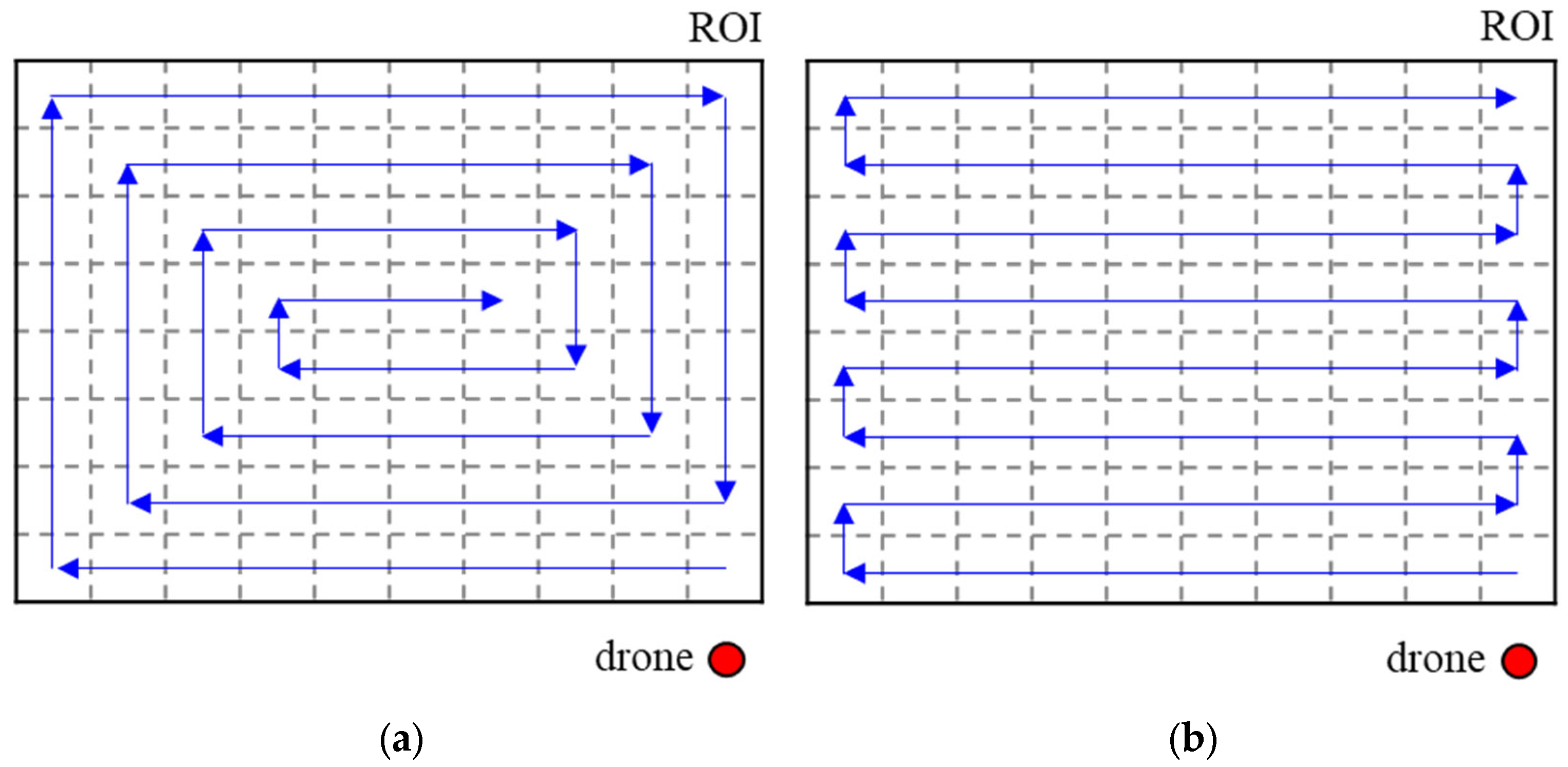
In general, the UAV performs the CPP through spiral and boustrophedon maneuvers [33]. The spiral maneuver is a method of flying inward by starting the circular flight from the outskirts of the ROI and gradually reducing the radius. The flight direction is set to either clockwise or counterclockwise. It takes a short return time compared to the boustrophedon method if the ROI area is small or there is enough flight time to scan the entire ROI at once. The boustrophedon maneuver is a flight method in which the drone gradually advances while sweeping left to right or up to down. Unlike the spiral maneuver, it has the advantage of gradually flying from a familiar area to an unknown area. Both methods can be applied regardless of the shape of the ROI; the flight patterns for both methods are depicted in Figure 1.

However, these two methods have two problems. Even if the entire ROI can be scanned in one flight, as shown in Figure 1, it is inefficient because the distance to return to the starting point is long. The other problem occurs when the ROI is huge or the maximum flight time of the drone is short. In this case, multiple flights are required to scan the entire ROI. In other words, multiple paths should be generated to cover the ROI. To generate multiple paths, methods of generating paths by applying the flight direction shown in Figure 1 or by dividing the ROI evenly can be considered. 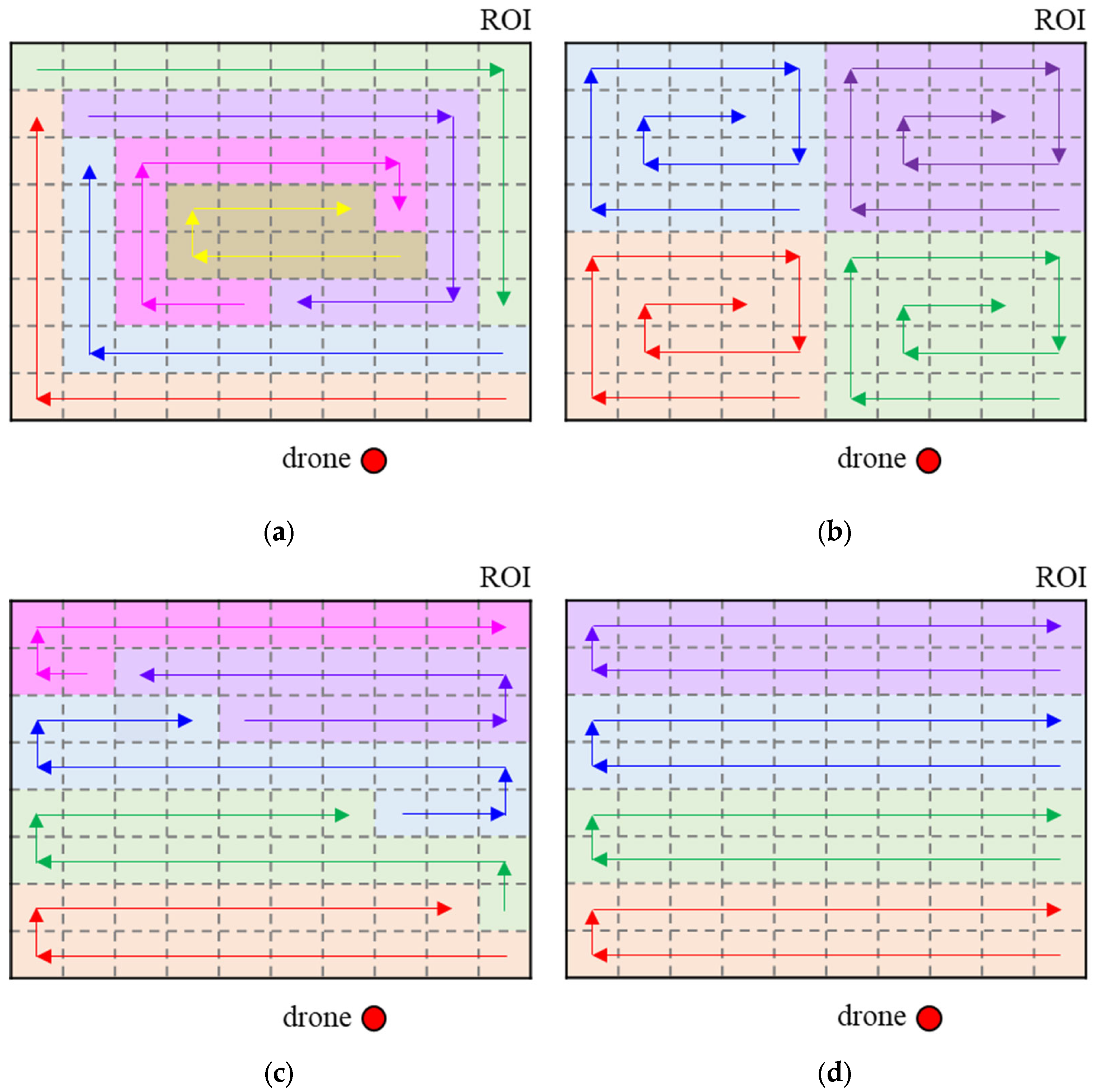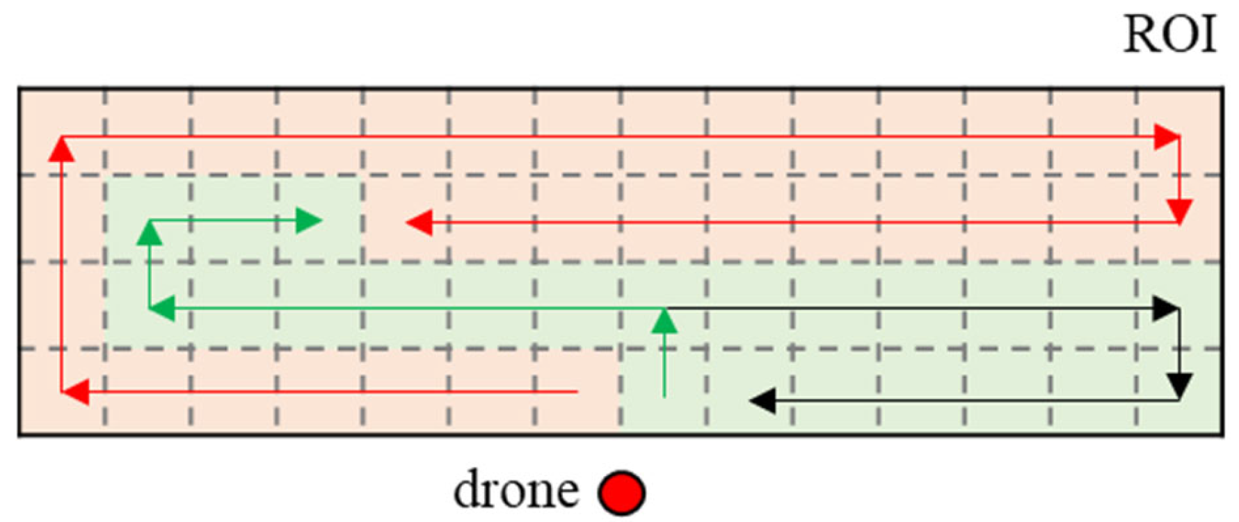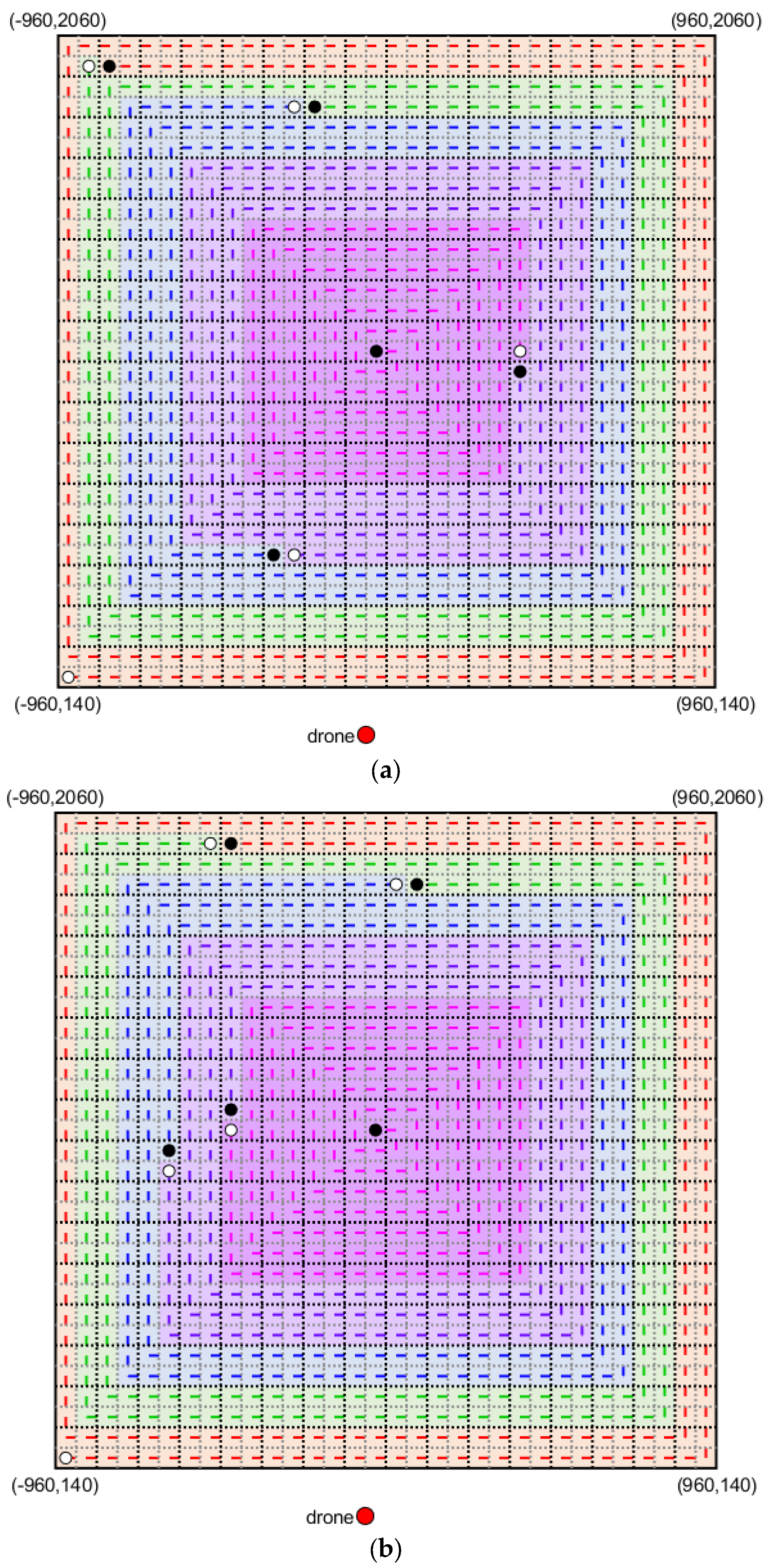Figure 2 shows the expected results when multiple paths are generated by the methods mentioned above, based on the spiral and boustrophedon maneuvers. Note that the color of the visited grids by each path is displayed differently in Figure 2. Also, the color of the flight directions for each path is depicted differently to distinguish between paths.

Figure 2a shows the expected CPP result considering the flight direction of spiral motion. The spiral motion derives a path starting from the outskirts of the ROI and gradually reducing the radius towards the center of the ROI. So, the drone scans along the red line on the outer edge of the ROI, starting from a corner grid close to the drone’s initial position. However, the drone can only scan a part of the ROI, so it has to return during the scan. After replacing the drone’s battery, the drone will scan along the green line on the outer edge of the remaining ROI, starting from where the red path ends since the drone should scan the ROI except for the red area. Following this procedure, the drone will fly along the lines in the following order: red, green, blue, purple, pink, and yellow. Note that the farther the distance from the drone’s initial position to the start/end grid of the scan, the smaller the number of grids that the drone can scan. So, the number of flights may increase unnecessarily to scan small unvisited areas if the drone flies using this method.

Figure 2b shows the expected CPP results by dividing the ROI evenly and using spiral motion. For CPP for multiple robots, a technique that simply divides the ROI area equally into the number of robots is widely used [34]. To apply this method, it assumes that the drone has enough maximum flight time to scan each divided area and return. Figure 2b shows the result of dividing the ROI into four equal-sized parts and generating paths through the spiral motion. As can be expected from the figure, the distance from the initial position of the drone to the start/end point of each path is different, so the time required to fly each path is different. This arrangement results in further increasing the time required to scan the entire ROI.

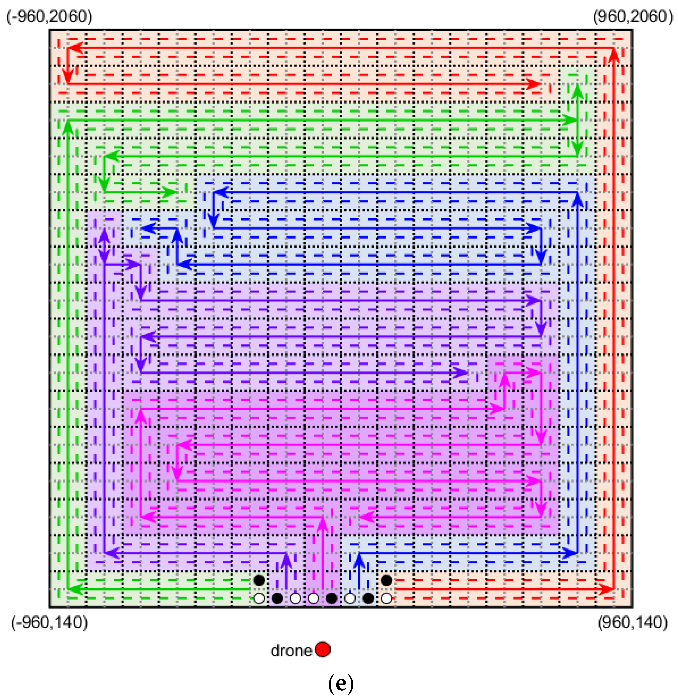
Figure 2c shows the expected CPP result considering the flight direction of boustrophedon motion. The boustrophedon motion creates a path that sweeps forward, starting from the ROI edge closest to the drone’s initial position. So, the drone scans along the red line on the bottom of the ROI, starting from a corner grid close to the drone’s initial position. However, the drone can only scan a part of the ROI, so it has to return during the scan. After replacing the drone’s battery, the drone will scan along the green line on the bottom of the remaining ROI starting from where the red path ends since the drone should scan the ROI except the red area. Following this procedure, the drone will fly along the lines in the following order: red, green, blue, purple, and pink. The farther the distance from the drone’s initial position to the start/end grid of the scan, the smaller the number of grids that the drone can scan, as shown in Figure 2a. So, the number of flights may also increase unnecessarily to scan small, unvisited areas.

Figure 2d shows the expected CPP results by dividing the ROI evenly and using boustrophedon motion. It also assumes that the drone has enough maximum flight time to scan each divided area and return. Figure 2d shows the result of dividing the ROI into four equal-sized parts and generating paths through the boustrophedon motion. As in Figure 2b, the distance from the initial position of the drone to the start/end point of each path is different, so the time required to fly each path is different. This arrangement results in further increasing the time required to scan the entire ROI.

As can be seen above, existing flight direction determination methods cannot be used to generate efficient multiple coverage paths. Therefore, a novel flight direction determination method to generate efficient multiple coverage paths is proposed. The proposed flight direction determination method is based on the basic rules for generating efficient coverage paths, which are described below. Note that DIP means the drone’s initial position in the rules.

Rule 1.

The closer the start and end grids of the path are to the DIP, the more efficient the path is since it increases the number of grids that can be scanned within the maximum flight time.

Rule 2.

The path is efficient to start the path from a grid close to the DIP, move away from the DIP, and then return to the vicinity of the DIP. If one path is only generated near the DIP, the efficiency of the path is good but the other paths are less efficient because they start and end far from the DIP.

Rule 3.

The path should be generated without any space. If the path is generated in a way that encloses some small spaces, it is necessary to fly once more to fill that empty space. It may increase the makespan to cover the whole ROI.

Rule 4.

The fewer paths are to cover the entire ROI, the more efficient the CPP. As the number of paths increases, the number of times the drone lands at the DIP increases. This means the time the drone does not perform a scan, which includes the time to fly from the DIP to the start point of the path, the time to return from the end of the path to the DIP, and the time to replace the drone’s battery from the DIP, increases.

Rule 5.

If the time required to cover the ROI is the same, reducing the maximum time required to fly along a path is effective when considering multiple drone operations. For example, if the time required to fly two paths is 10 s and 5 s, respectively, the time required to operate one drone is 15 s plus battery replacement time while the time required to operate two drones is 10 s only. If the time required to scan the same area is 7.5 s for both paths, the time required to operate one drone is the same, but the time required to operate two drones is 7.5 s.

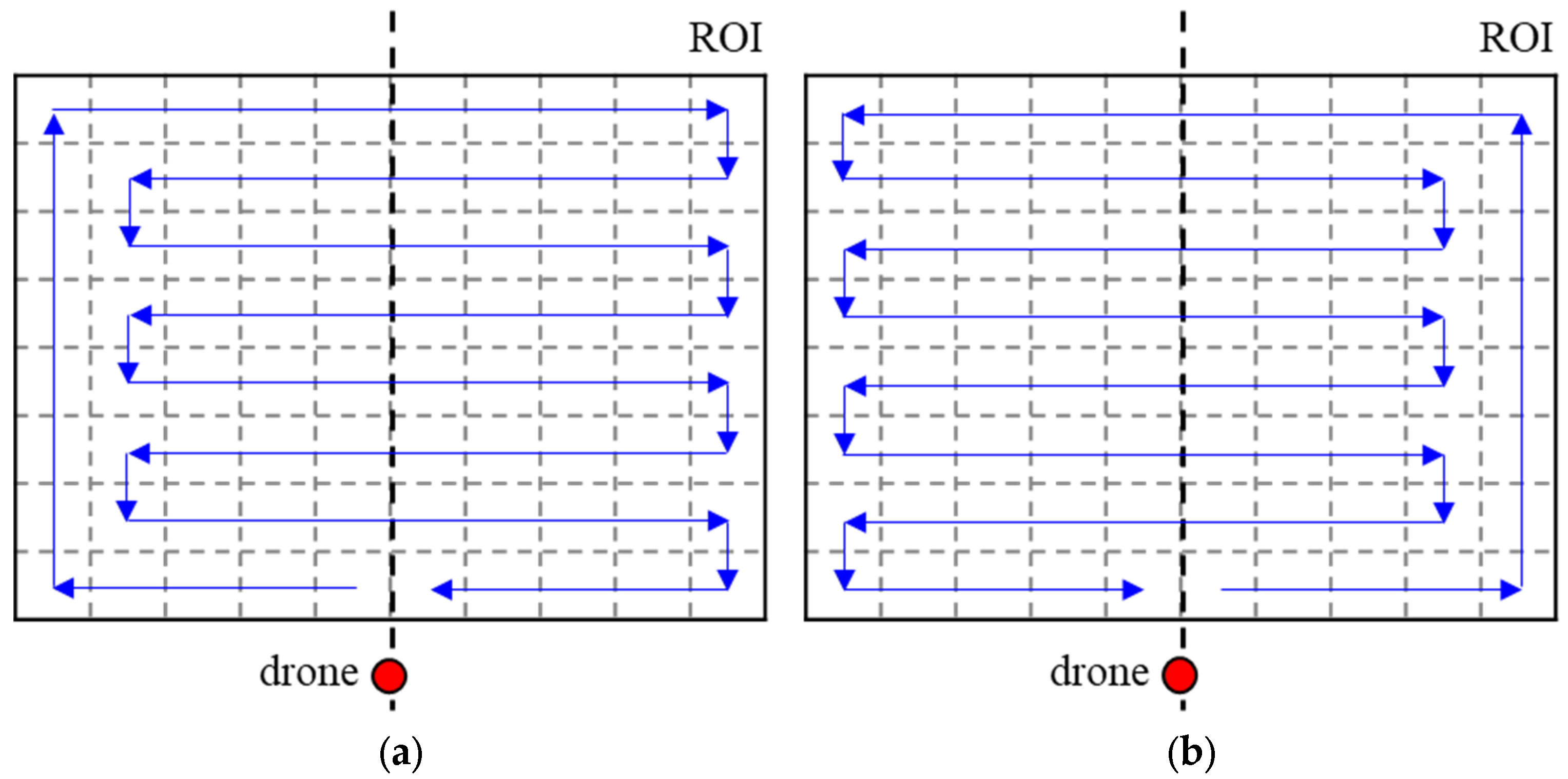
As seen in Rules 1, 2, and 4, the initial position of the drone should be considered for deriving an efficient flight direction. Figure 3 shows the proposed flight direction of the drone considering the drone’s initial position.

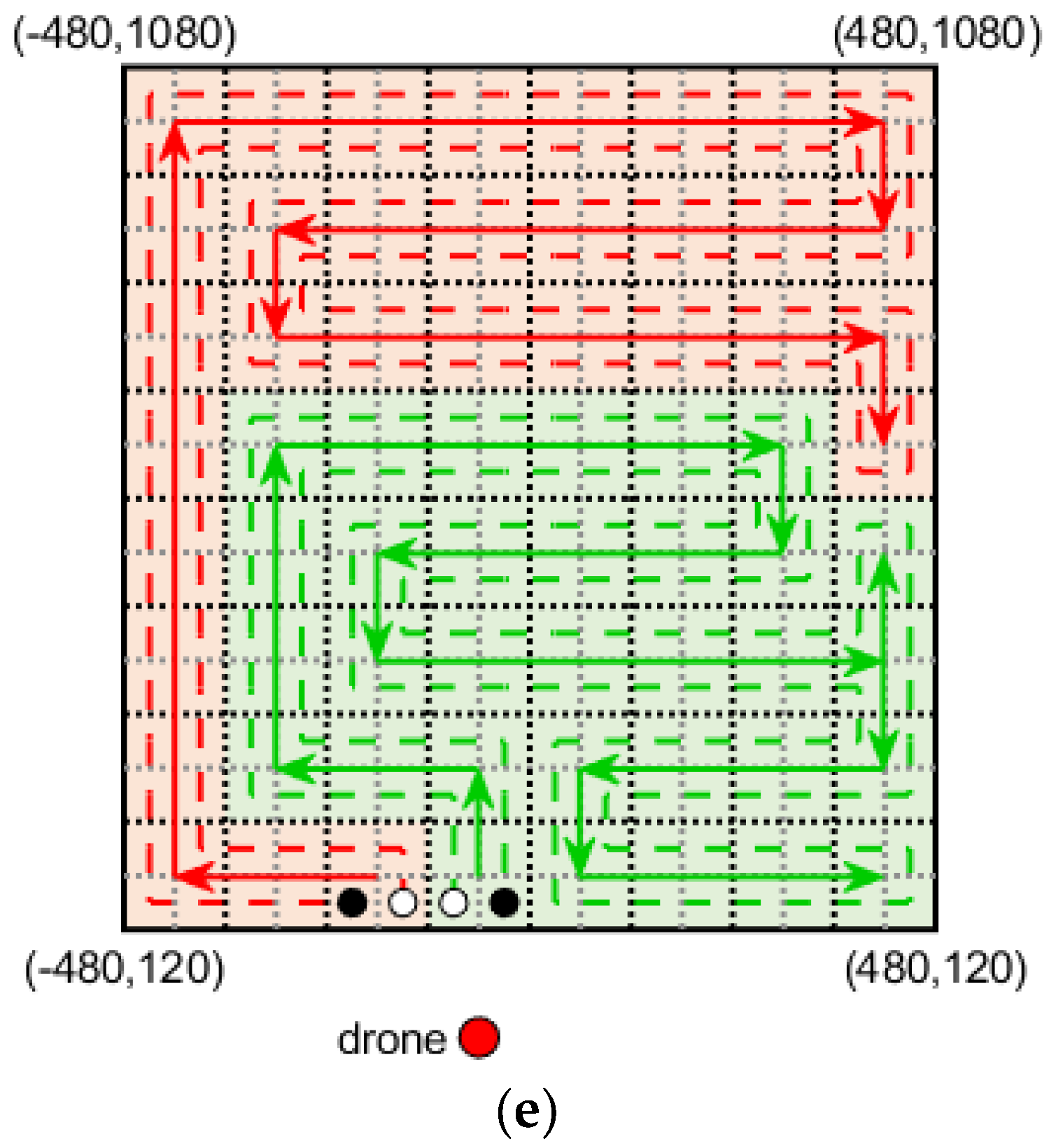
According to Rule 1, each path should start near the initial position of the drone. The fifth and sixth grids in the bottom row of the ROI can be selected as the initial position. If the fifth grid is selected as the first grid of the path, the flight direction is made, as shown in Figure 3a. The drone should start near the initial position of the drone and move away from it, as mentioned in Rule 2, so it will fly along the bottom side of the ROI and then go up along the left side. This part is similar to the spiral motion in Figure 1a. When the drone reaches the upper left, it will fly to the right to scan the upper edge, which is the farthest from the drone’s initial position. The drone will go down one grid and then fly to the left since there should be no empty grid while scanning, according to Rule 3. To avoid creating empty grids, the drone will fly in the same way as the boustrophedon maneuver in Figure 1b, afterward. Figure 3a can be derived by setting the priority of directions to left > up > right > down. When flying to the left from the first grid and reaching the left side of the ROI, it is impossible to fly to the left so the drone will fly upward, which is the next priority. If the drone reaches the upper side of the ROI, it cannot fly to the left or upward so it flies to the right, which is the next priority. Since the drone cannot fly to a grid that has already been visited, it can reach the right side of the ROI. Then, the drone cannot fly to the left, up, or right, so it will move downward, which is the last priority. When the drone goes down one grid, there are unvisited grids on the left, so it will fly to the left. If the sixth grid in the bottom of the ROI is selected as the first grid of the path, the flight direction is made, as shown in Figure 3b, following the same logic as explained above. In that case, the priority of directions is set to right > up > left > down. If the drone can scan the whole ROI through one flight, flying in this way satisfies rules 1 and 2 because the final position of the path will be near the drone’s initial position. Note that even if the initial position of the drone is not at the bottom of the ROI, the direction priority can be set by referring to Figure 3.

4.2. Main Algorithm

Once the drone’s flight direction has been determined, multiple paths for covering the ROI should be created based on it. The proposed CPP algorithm consists of five steps: ROI adjustment, initial GRID selection, GRID path generation, rebalancing multiple path, and multiple coverage paths generation. The meaning of the word ”GRID” will be explained in Section 4.2.1.

4.2.1. Adjust Region of Interest

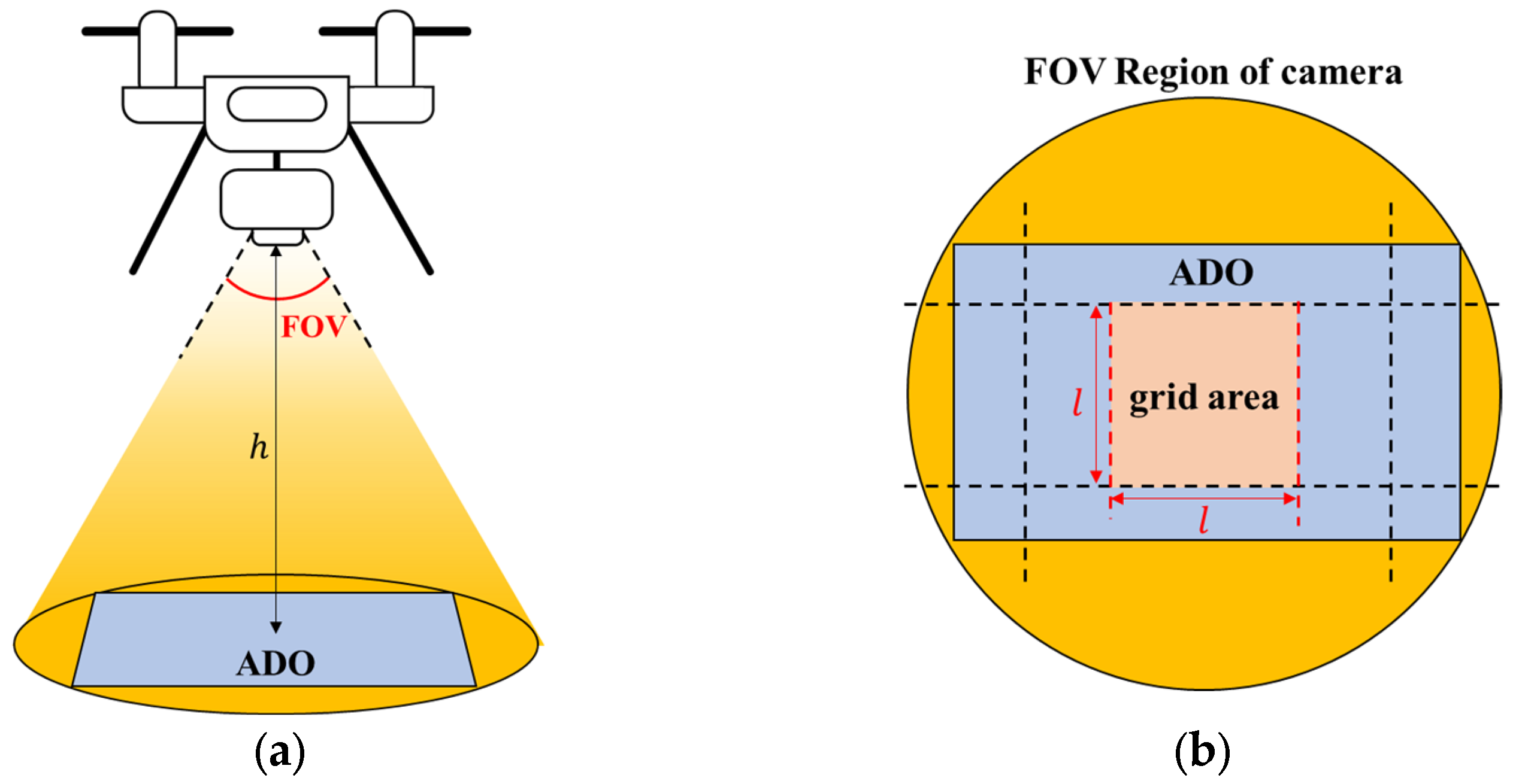
When the ROI is set by the user, the ROI should be divided into several small grids to generate coverage paths based on the ADO. If there is no overlap between the captured areas, it is impossible to confirm whether the photos were taken at the desired position and the photos cannot be aligned. Therefore, the grid is generally set to be smaller than the ADO, considering the overlap rate between the photos, as depicted in Figure 4 [35].

The ADO is determined as the largest rectangular area within the area determined by the FOV of the camera mounted on the drone and the height of the camera, as shown in Figure 4a. The ratio of the rectangular ADO is determined by the ratio of the image sensor in the camera. Figure 4b shows the areas when viewed directly downward. The yellow circle and blue rectangle mean the FOV region of the camera and the ADO, respectively. If the ADO is reduced by the overlap ratio, a rectangular area created by four black dashed lines is derived. If the rectangular area is set to a grid area, the distance to the next grid will vary depending on the flight direction. Therefore, the square area created based on the short side of the rectangular area, indicated by the red square in Figure 4b, is set as the grid area.

Once the grid size is determined, the ROI can be divided into grids. If the path is generated by simply dividing the ROI into grids, it is not guaranteed that the last grid of the path will be near the initial position of the drone even if the proposed flight direction is applied. Therefore, a GRID is formed by combining four grids $(2 \times 2)$, and the area of the ROI is adjusted so that the ROI is exactly divided into the GRID to guarantee the return path. The pseudo-code for the ROI adjustment step is described in Algorithm 1.

Algorithm 1. ROI Adjustment step
1:	input $\left[\left(x_1,y_1\right), \left(x_2,y_2\right)\right], h, {\theta }_{FOV}, {\rho }_{img},{\gamma }_{ovlp}$
2:	$d_{ADO}=2h\tan \left({\theta }_{FOV}/2\right)$
3:	$w_{ADO}=d_{ADO}·{\rho }_{img}(1)/‖{\rho }_{img}‖$, $h_{ADO}=d_{ADO}·{\rho }_{img}(2)/‖{\rho }_{img}‖$
4:	$w_{grid}=h_{grid}=\left(1-{\gamma }_{ovlp}\right)·\min (w_{ADO},h_{ADO})$
5:	$w_{GRID}=h_{GRID}=2w_{grid}$
6:	$w_{ROI}=x_2-x_1$, $h_{ROI}=y_2-y_1$
7:	$r=\left[\mathrm{r}\mathrm{e}\mathrm{m}\left(w_{ROI},w_{GRID}\right),\mathrm{r}\mathrm{e}\mathrm{m}(h_{ROI},h_{GRID})\right]$
8:	if $r\left(1\right)!=0$
9:	if  $r\left(1\right)>w_{GRID}-r\left(1\right)$
10:	$w_{ROI}=\left\{\mathrm{f}\mathrm{i}\mathrm{x}\left(w_{ROI}/w_{GRID}\right)+1\right\}·w_{GRID}$
11:	$x_1=x_1-\left(w_{GRID}-r\left(1\right)\right)/2$, $x_2=x_2+\left(w_{GRID}-r\left(1\right)\right)/2$
12:	else
13:	$w_{ROI}=\mathrm{f}\mathrm{i}\mathrm{x}\left(w_{ROI}/w_{GRID}\right)·w_{GRID}$
14:	$x_1=x_1+r\left(1\right)/2$, $x_2=x_2-r\left(1\right)/2$
15:	end if
16:	end if
17:	if $r\left(2\right) !=0$
18:	if  $r\left(2\right)>w_{GRID}-r\left(2\right)$
19:	$h_{ROI}=\left\{\mathrm{f}\mathrm{i}\mathrm{x}\left(h_{ROI}/h_{GRID}\right)+1\right\}·h_{GRID}$
20:	$y_1=y_1-\left(h_{GRID}-r\left(2\right)\right)/2$, $y_2=y_2+\left(h_{GRID}-r\left(2\right)\right)/2$
21:	else
22:	$h_{ROI}=\mathrm{f}\mathrm{i}\mathrm{x}\left(h_{ROI}/h_{GRID}\right)·h_{GRID}$
23:	$y_1=y_1+r\left(2\right)/2$, $y_2=y_2-r\left(2\right)/2$
24:	end if
25:	end if
26:	$N_{grid}=(2·w_{ROI}/w_{grid})\times (2·h_{ROI}/h_{grid})$

In line 1, the inputs are received from the user to generate paths for covering the ROI, where $\left(x_1,y_1\right)$ and $\left(x_2,y_2\right)$ are the lower left and upper right coordinates of the ROI, respectively; $h$ is the height of drone operation; ${\theta }_{FOV}$ is the camera FOV angle; ${\rho }_{img}$ is the ratio of image sensor’s size of the camera; and ${\gamma }_{ovlp}$ is the overlap rate. Then, the size of the ADO is calculated through lines 2–3, where $d_{ADO}$ is the diagonal length of the ADO, and $w_{ADO}$ and $h_{ADO}$ are the width and height of the ADO, respectively. In line 4, the size of the grid is calculated by reducing the short side of the ADO by the overlap ratio, where $w_{grid}$ and $h_{grid}$ are the width and height of the grid, respectively. The size of the GRID is calculated by doubling the width and height of the grid in line 5, where $w_{GRID}$ and $h_{GRID}$ are the width and height of the GRID, respectively. In line 6, the initial size of the ROI is calculated, where $w_{ROI}$ and $h_{ROI}$ are the width and height of the ROI, respectively. If $w_{ROI}$ and $h_{ROI}$ are not multiples of $w_{GRID}$ and $h_{GRID}$, respectively, the size of the ROI is adjusted to make $w_{ROI}$ and $h_{ROI}$ multiples of $w_{GRID}$ and $h_{GRID}$, respectively, through lines 8–25. For each of the horizontal and vertical axes, the sizes of the adjustment values for increasing and decreasing the ROI are compared, and the adjustment is performed in a smaller direction. Then, $N_{grid}$ in Equations (1) and (6) can be calculated as described in line 26.

4.2.2. Initial GRID Selection

Once the size of the ROI is adjusted, the number of paths required to scan the entire ROI is roughly estimated. The maximum number of GRIDs that can be scanned within the drone’s maximum flight time is calculated assuming that the drone starts from the GRID closest to its initial position and ends at that GRID, and then returns to its initial position. The number of paths required to scan the entire area is roughly calculated by dividing the total number of GRIDs by the maximum number of GRIDs derived previously. Note that the number of GRIDs that a drone can scan in one flight and the number of paths required to scan the entire ROI are adjusted in the subsequent algorithms.

After determining the approximate number of paths, a determined number of paths that cover the entire ROI should be created. According to Rule 1, the closer the starting grid of the path is to the initial position of the drone, the better. If a method that first selects the starting GRIDs of all paths close to the drone’s initial position and then completes the paths sequentially is used, it may hinder the progress of each path during the step for generating multiple coverage paths. Therefore, the proposed algorithm uses a method of generating the next path after completely generating one path. To generate each path, an initial GRID should be selected first, and then the GRID path should be generated according to the maneuver methods specified in Section 4.1. The method of selecting the initial GRID of the path is presented in pseudo-code in Algorithm 2.

Algorithm 2. Initial GRID selection
1:	$\mathit{l}={\infty }_{1\times n}$$, \mathit{d}={\infty }_{1\times n}$, n = # of horizontal GRIDs in ROI
2:	for i = 1: n
3:	$\mathit{l}\left(i\right)={argmin}_m \left\{own\left(i,m\right)==0\right\}$
4:	$\mathit{d}\left(i\right)=dist(\left(x_{DIP},y_{DIP}\right),\left(x_i,y_{\mathit{l}\left(i\right)}\right))$
5:	end for
6:	Sort $(\mathit{d}, \mathrm{ascending} \mathrm{order})$
7:	$I_x={argmax}_{column} \mathit{d}$(1: # of reserved GRID path), $I_y=\mathit{l}\left(I_x\right)$

In line 1, the index list $l$ and the distance vector $d$, which have as many elements as the number of horizontal GRIDs of the ROI, are initialized, where $n$ is the number of horizontal GRIDs in the ROI. In lines 2~5, the unassigned GRID that is close to the initial position of the drone in each column is found, and the distance from the initial position of the drone to that GRID is calculated, where $\left(x_{DIP},y_{DIP}\right)$ and $\left(x_i,y_{l\left(i\right)}\right)$ are the initial position of the drone and the position of the GRID, respectively. The calculated distance vector is sorted in ascending order in line 6, and the column with the largest value in the top $k$ of the generated vector is found, where $k$ is the number of GRID paths that are not generated in line 7. The smallest unassigned row in that column is selected as the first GRID of the path, where $I_x$ and $I_y$ are the horizontal and vertical index when the ROI is divided into GRIDs, respectively. Note that Algorithm 2 is used when the initial position of the drone is at the bottom of the ROI and can be applied by modifying line 3 if the initial position is in a different direction of the ROI.

4.2.3. Make GRID Path

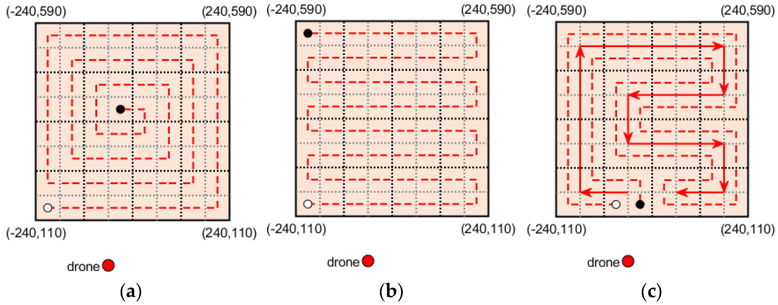
After the starting GRID of a path is determined, the remaining path of the GRID should be generated taking into account the maximum flight time of the drone. The GRID path can be expended in four directions (up, down, left, right), and furcating is possible from the previously visited GRID if the path is blocked, as shown in Figure 5. The reason is to create a GRID path-based grid path that starts from the initial GRID, flies the path in four directions, and then returns to the initial GRID.

In Figure 5, it is assumed that the path of the red line passing through all the red GRIDs is generated first. Since the red path does not cover the entire ROI, the green line path is additionally generated based on the flight direction described in Section 4.1. However, the green path is blocked by the previously generated path. So, the black path is generated by branching from the previously visited GRID. GRID paths that cover the entire ROI are generated through this procedure. The procedure to extend the GRID path according to the flight direction, as defined in Section 4.1, is described in Algorithm 3.

Algorithm 3. Make GRID path
1:	$\Delta t=4\left(l_{grid}/v_h+t_h\right)$
2:	$\mathbf{while} (\mathrm{makespan} \mathrm{of} \mathrm{GRID} \mathrm{path} < t_{max}$)
3:	$\mathbf{if} x_1<x_{DIP}$
4:	priority = [left, up, right, down]
5:	else
6:	priority = [right, up, left, down]
7:	end if
8:	$\mathbf{if} (\mathrm{makespan} \mathrm{of} \mathrm{GRID} \mathrm{path})+\Delta t<t_{max}$
9:	AddOneGRIDtoEnd(priority)
10:	if not added
11:	AddOneGRIDtoMiddle (priority)
12:	end if
13:	end if
14:	if not added
15:	AddOneGRIDtoFirst (priority_inverse)
16:	end if
17:	if added
18:	Calculate Makespan
19:	else
20:	break
21:	end if
22:	end while

A GRID path is created by sequentially adding GRIDs one by one until no more GRIDs can be added to the current path. In line 1, the incremental time when a GRID is added is calculated, where $l_{grid}$ is the length of one side of the grid, $v_h$ is the horizontal velocity of the drone, and $t_h$ is the hovering time at the center of the grid. In lines 3~7, as explained in Section 4.1, the priority is set to left > up > right > down if the initial GRID position is to the left of the drone’s initial position, or it is set to right > up > left > down otherwise, where $x_1$ means the $x$ coordinate values of the initial GRID. If the makespan does not exceed the drone’s maximum flight time when one GRID is added to the path, adding one GRID at the end of the path is tried first in line 9, based on the priority in lines 4 or 6. If adding one GRID fails, adding one GRID by furcating the previously visited GRIDs is tried based on the priority. This procedure is also based on the determined priority. If this also fails, adding one GRID before the starting GRID of the path is tried in line 15. Note that the priority used here is the inverse of the priority determined in lines 4 or 6. Here, the inverse means swapping left and right, up and down, respectively. For example, the inverse priority will be right > down > left > up if the priority is left > up > right > down. It should be added with inverse priority before the first GRID of the path so that the previously created path is added to the changed starting GRID with the determined priority. If a GRID is added to the path, the makespan is calculated in line 18. Note that the makespan simply increases by $\Delta t$ if a GRID is added by line 9 or 11, but if a GRID is added in line 18, the starting GRID changes, so the time to go back and forth from the drone’s initial position to the starting GRID changes, requiring recalculation of the makespan. If a GRID cannot be added to the path, the path extension is stopped and the loop is exited in line 20.

4.2.4. Rebalancing

If the number of paths roughly determined in Section 4.2.2 is not enough to cover the entire ROI, the number of paths is increased by one, and Algorithms 2 and 3 are performed again. This process is to minimize the number of paths to cover the entire ROI, as mentioned in Rule 4. When multiple paths covering the entire ROI are generated through this procedure, the generated paths are rebalanced to find the optimal solution according to Rule 5. The rebalancing process is to repeatedly remove one GRID from the path with the largest makespan and give it to the path with the smallest makespan, as described in Algorithm 4.

Algorithm 4. Rebalancing
1:	$\Delta t=4\left(l_{grid}/v_h+t_h\right)$
2:	while true
3:	${makespan}_{tmp}=makespan$
4:	$makespa{n}_{bfr}=sort(makespa{n}_{tmp},’descend’)$
5:	$p_{max}^G={argmax}_i makespa{n}_{tmp}\left(i\right)$
6:	$p_{min}^G={argmin}_i makespa{n}_{tmp}\left(i\right)$
7:	$makespa{n}_{tmp}\left(p_{max}^G\right)=makespa{n}_{tmp}\left(p_{max}^G\right)-\Delta t$
8:	$makespa{n}_{tmp}\left(p_{min}^G\right)=makespa{n}_{tmp}\left(p_{min}^G\right)+\Delta t$
9:	$makespa{n}_{aftr}=sort(makespa{n}_{tmp},’descend’)$
10:	for i = 1:$n_{p,G}$
11:	if $makespa{n}_{bfr}\left(i\right)>makespa{n}_{aftr}\left(i\right)$
12:	$n_{p_{max}}^G=n_{p_{max}}^G-1$
13:	$n_{p_{min}}^G=n_{p_{min}}^G+1$
14:	$makespan={makespan}_{tmp}$
15:	break
16:	else if $makespa{n}_{bfr}\left(i\right)<makespa{n}_{aftr}\left(i\right)$
17:	break
18:	end if
19:	end for
20:	if makespan did not changed
21:	break
22:	end if
23:	end while

In line 1, the incremental time when a GRID is added to a GRID path is calculated, as in line 1 of Algorithm 3. In line 3, the makespans are copied to ${makespan}_{tmp}$ for further processing. In lines 4~6, ${makespan}_{tmp}$ is sorted in descending order to find path $p_{max}^G$, which has the largest makespan, and path $p_{min}^G$, which has the smallest makespan. The makespans that are changed when a GRID is removed from $p_{max}^G$ and given to $p_{min}^G$ is calculated in lines 7~8. The changed makespans are also sorted in descending order to compare with $makespa{n}_{bfr}$ in line 9. In lines 10~19, $makespa{n}_{aftr}$ is compared with $makespa{n}_{bfr}$ for each element to check whether $makespa{n}_{aftr}$ is more efficient than the previous makespan, where $n_{p,G}$ means the number of GRID paths. If it is better than the previous one, the number of GRIDs in $p_{max}^G$ and $p_{min}^G$ are adjusted and the makespan is renewed, where $n_{p_{max}}^G$ and $n_{p_{min}}^G$ are the number of GRIDs in $p_{max}^G$ and $p_{min}^G$, respectively. If not, the previous solution is maintained. In line 21, the while loop is exited if there is no change in the makespan. After that, Algorithm 3 is run so that each path is assigned the number of GRIDs derived from Algorithm 4.

4.2.5. Make Multiple Coverage Paths

Once multiple GRID paths covering the entire ROI are created, a grid path should be generated based on each GRID path. The grid path is created in a way that surrounds the GRID path. In other words, the grid path starts from the starting GRID, reaches the last GRID, and then returns to the starting GRID. Since the starting GRID is selected close to the initial position of the drone, the grid path satisfies Rule 2 described in Section 4.1. The method of generating a grid path based on the GRID path is described in Algorithm 5.

Algorithm 5. Make Multiple Coverage Paths
1:	for i = 1:$n_{p,G}$
2:	for j = 1:$n_{p_i}^G$
3:	if $j==1$
4:	${\mathit{g}}_{i,1}=Grid2grids(p_{i,1}^G)$
5:	${\mathit{d}}_{i,1}=norm(p_{DIP}-{\mathit{g}}_{i,1})$
6:	$p_{i,1}^g=\mathrm{shortest} \mathrm{grid} \mathrm{in} {\mathit{d}}_{i,1}$
7:	$p_{i,4}^g=\mathrm{second} \mathrm{shortest} \mathrm{grid} \mathrm{in} {\mathit{d}}_{i,1}$
8:	$set p_{i,2}^g \mathrm{and} p_{i,3}^g \mathrm{to} \mathrm{connect} p_{i,1}^g \mathrm{and} p_{i,4}^g$
9:	else if $p_{i,(j-1)}^G$ and $p_{i,j}^G$ are neighbors each other
10:	${\mathit{g}}_{i,j}=Grid2grids\left(p_{i,j}^G\right)$
11:	insert ${\mathit{g}}_{i,j}$ near the path associated with $p_{i,(j-1)}^G$ among ${\mathit{p}}_i^g$
12:	else
13:	find $p_{i,\left(j-a\right)}^G$ where $p_{i,\left(j-a\right)}^G$ and $p_{i,j}^G$ are neighbors each other, $0<a<j$
14:	${\mathit{g}}_{i,j}=Grid2grids(p_{i,j}^G)$
15:	insert ${\mathit{g}}_{i,j}$ near the path associated with $p_{i,\left(j-a\right)}^G$ among ${\mathit{p}}_i^g$
16:	end if
17:	end for
18:	end for

In lines 3~16, a grid path is expended sequentially along the GRID path. If the selected GRID is the first GRID in the GRID path, ${\mathit{g}}_{i,1}$, the positions of four grids, are calculated based on the GRID $p_{i,1}^G$ in line 4. The distance from each grid to the initial position of the drone is calculated in line 5, where ${\mathit{d}}_{i,1}$ is the distance vector from each grid to the initial position of the drone. 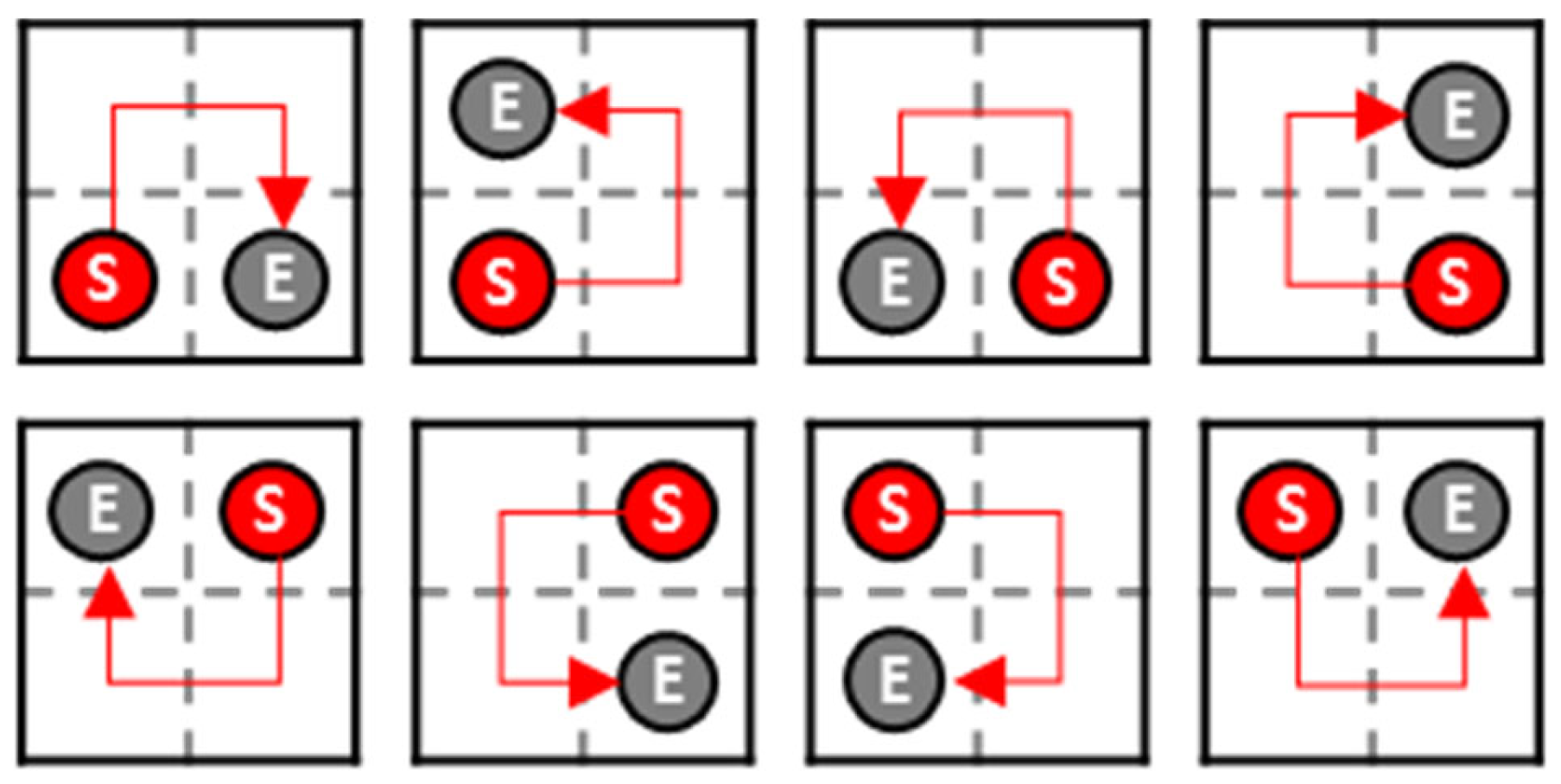The two shortest grids are set as the start and end points of the path, $p_{i,1}^g$ and $p_{i,4}^g$, in lines 6~7. Note that the fourth grid becomes the endpoint if a path is generated for the first GRID since one GRID consists of four grids. The grid path is generated in line 8 by determining the order of the remaining two grids so that they can reach the end point by moving only up, down, left, and right sequentially from the start point, as shown in Figure 6.

Here, the square with a black border represents the first GRID of the GRID path. The four squares divided by gray dashed lines represent grids. The red circle with ”S” and the gray circle with ”E” represent the start and end points of the grid path, respectively. Figure 6 shows the results of grid path generation for all cases where the start and end points of the grid path can be selected from the first GRID, represented by red arrows. From the second GRID in the GRID path onwards, it is checked whether the previous GRID and the current GRID are neighbors. Here, neighbor means that the distance between the centers of the two GRIDs matches the length of a side of the GRID. If they adjoin each other, the current GRID is divided into four grids, and the path that visits all the generated grids is inserted near the path associated with the previous GRID among the existing grid path in lines 10~11, where $p_{i,(j-1)}^G$, $p_{i,j}^G$, and ${\mathit{p}}_i^g$ mean the previous GRID, the current GRID, and the existing grid path, respectively. If they do not adjoin each other, a GRID $p_{i,\left(j-a\right)}^G$ that is adjacent to the current GRID is found by going back from the previous GRID in the GRID path until it reaches the neighboring GRID of the current GRID in line 13. The current GRID is divided into four grids in line 14, and they are inserted near the path associated with $p_{i,\left(j-a\right)}^G$ among ${\mathit{p}}_i^g$ in line 15. 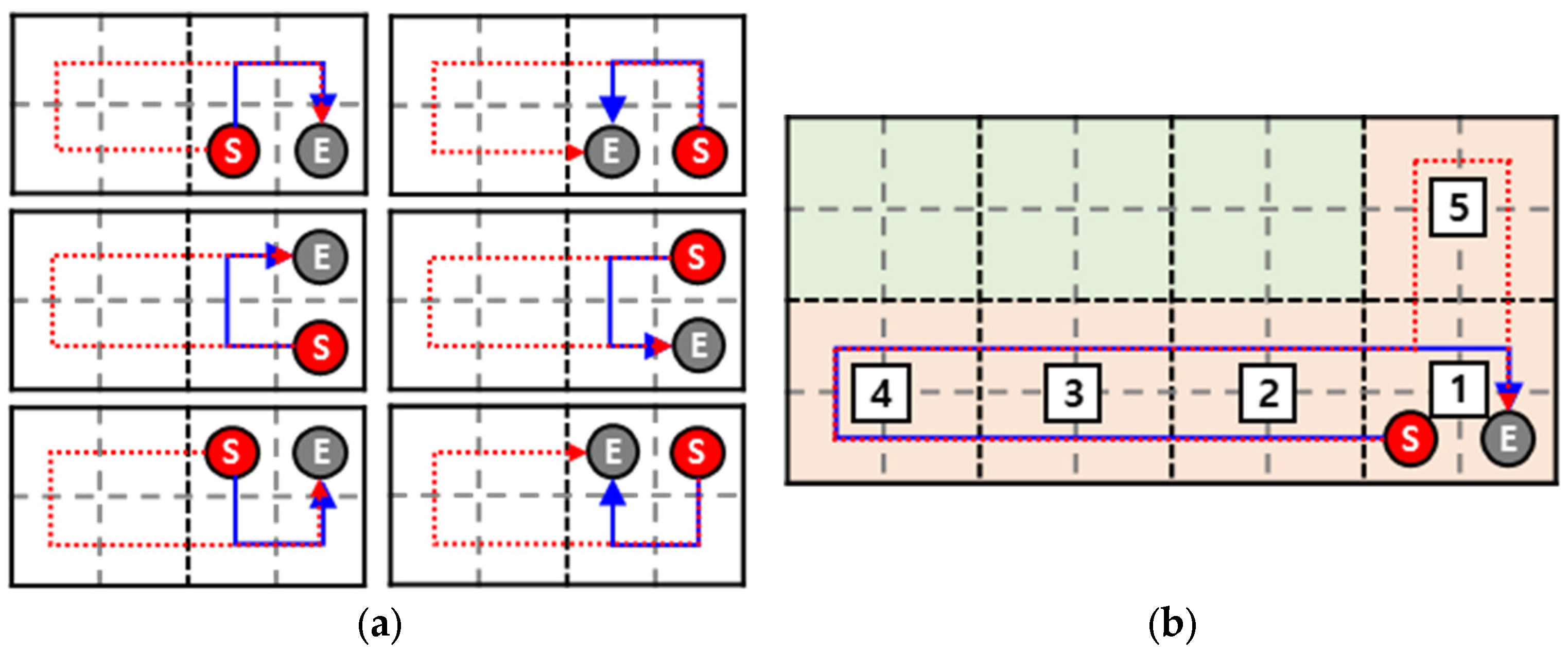Figure 7 shows an example of grid path generation when the previous GRID and the current GRID are neighbors and when they are not.

In Figure 7, the blue line and the red dotted line mean before and after generating the grid path for the current GRID, respectively. In Figure 7a, it is assumed that the first and the second GRIDs in the GRID path are the GRIDs on the right and left, respectively. The second GRID is divided into four grids in line 10 of Algorithm 5, as shown as the left GRID in Figure 7a. Then, the red-dotted grid path is generated in line 11. Note that the red dotted path starts from the starting point, visits the entire grid generated by line 10, and reaches the endpoint by only moving up, down, left, and right. In Figure 7b, it is assumed that the top three GRIDs are occupied by another GRID path. Then, the GRID path will be made in the order of the numbers written in the white box. Note that the fifth GRID is added by furcating from the first GRID. In line 13 of Algorithm 5, the adjacent GRID to the fifth GRID is found starting from the fourth GRID and going backward. The first GRID will be found to be adjacent to the fifth GRID, and four grids generated by dividing the current GRID in line 14 are added near the path associated with the first GRID in the existing grid path in line 15. As a result, the existing blue path is updated to a red dotted path. The whole pseudo-code of the proposed multi-CPP algorithm is shown in Algorithm 6.

Algorithm 6. Proposed Multi-CPP Algorithm
1:	run Algorithm 1 to adjust the ROI
2:	decide the number of GRID path $n_{p,G}(=N_p)$ roughly to cover the ROI
3:	while true
4:	for i = 1:$n_{p,G}$
5:	run Algorithm 2 to select the initial GRID for GRID path ${\mathit{p}}_i^G$
6:	run Algorithm 3 to generate the GRID path ${\mathit{p}}_i^G$
7:	end for
8:	if there are unvisited GRIDs
9:	$n_{p,G}=n_{p,G}+1$
10:	else
11:	run Algorithm 4 for rebalancing
12:	initialize all GRIDs except the first GRID of each path
13:	for i = 1:$n_{p,G}$
14:	run Algorithm 3 to generate the GRID path ${\mathit{p}}_i^G$ which has the number of                     GRIDs determined in Algorithm 4
15:	end for
16:	break
17:	end if
18:	end while
19:	run Algorithm 5 to generate grid paths

When the user inputs for CPP are received, Algorithm 1 is run to adjust the ROI in line 1. Once the ROI adjustment is complete, the number of GRID paths $n_{p,G}$ is roughly determined in line 2 based on the GRID size determined in Algorithm 1 and the initial position of the drone. The GRID paths are generated in lines 5~6, as many as $n_{p,G}$, and it is checked whether the generated GRID paths cover the entire ROI. If not, $n_{p,G}$ is increased by 1, and lines 5~6 are performed until the generated GRID paths cover the entire ROI. If the entire ROI is covered by the paths, Algorithm 4 is run for rebalancing the paths. In line 12, each GRID path is initialized, leaving only the initial GRID. Then, a GRID path with a path length equal to the number of GRIDs determined in Algorithm 4 is generated sequentially in lines 13~15. Once the GRID paths covering the entire ROI are generated, Algorithm 5 is run to generate multiple grid paths, which are the results of the proposed algorithm.

5. Simulation Results

To evaluate the performance of the proposed algorithm, simulations are performed in three environments: a 0.5 km × 0.5 km environment where the drone can scan the entire ROI at once, a 1 km × 1 km environment where the drone needs to fly twice to scan the ROI, and 2 km × 2 km environment where the drone needs to make several flights. The input parameters for each of the three environments are shown in

Table 1. The input parameters for each of the three environments.

	Case 1	Case 2	Case 3
ROI pos. [m]	(−250,100), (250,600)	(−500,100), (500,1100)	(−1000,100), (1000,2100)
Drone pos. [m]	(−60,0)	(−60,0)	(−60,0)
Drone vel. [m/s]	takeoff: 2.0 landing: 2.0 scanning: 6.0 horizontal: 15.0	takeoff: 2.0 landing: 2.0 scanning: 6.0 horizontal: 15.0	takeoff: 2.0 landing: 2.0 scanning: 6.0 horizontal: 15.0
Max. flight time [s]	2400	2400	2400
Flight height [m] (AGL)	100	100	100 [m]
Camera FOV [deg]	75	75	75
Image ratio	16/9	16/9	16/9
Overlap rate [%]	20	20	20

. Note that the remaining inputs are the same except for the ROI position.

Here, the ROI position represents the coordinates of the lower left and upper right of the rectangular ROI, respectively. The drone’s position means the initial position and the drone should return to that position if multiple flights are required. The drone’s speed is composed of the speed during takeoff, landing, scanning, and horizontal flight. Horizontal flight means the movement to the start or end of a grid path. The drone’s maximum flight time and flight height are set to 2400 s and 100 m above the ground level (AGL), respectively. The ground surface is assumed to be flat in the simulation environments, so the height will be maintained until landing once it takes off. The FOV and image ratio of the camera are set to 75 degrees and 16:9, respectively. The overlap rate between the pictures captured by the camera is set to 20%. If the size of the grid is calculated as described in Algorithm 1, the length of one side of the grid will be 60 m. The length of one side of the GRID is twice that of the grid, so it becomes 120 m. The simulations were run in MATLAB, and the computer and software specifications are described in

Table 2. The computer and software specifications for simulations.

Contents	Specification
CPU	Intel® CoreTM i5-10500 3.10 GHz (6 cores, 12 threads)
GPU	Intel® UHD Graphics 630
RAM	16 GB
Storage	256 GB SSD
Software	MATLAB 2018b

.

The simulation results of the proposed algorithm are presented with the results of spiral motion and boustrophedon motion, which are widely used, for performance comparison.

5.1. Simulation Results for Case 1

Case 1 requires scanning an ROI of 0.5 km × 0.5 km, and the simulation results are shown in Figure 8 and

Table 3. Information about the generated path for case 1 and each CPP calculation method.

Method	Path Number	Moving Distance	# of Grids in Path	Makespan	Calculation Time
Spiral	1	4566.3652 m	64	769.0910 s	0.0225 s
Boustrophedon	1	4764.9242 m	64	782.3283 s	0.0107 s
Proposed	1	4266.3564 m	64	749.0904 s	0.0588 s

.

In Figure 8, the area marked with black solid lines represents the adjusted ROI. Note that the coordinates of the lower left and upper right of the ROI were adjusted from (−250,100) and (250,600) to (−240,110) and (240,590), respectively, by Algorithm 1, which results in a reduction in the ROI. The area divided by the black dotted lines and gray dotted lines in the ROI represent the GRID and grid, respectively. The red dashed line is the coverage path generated by each CPP method. The white and black circles mean the start and end grids of the coverage path, respectively. Figure 8a shows the coverage path generated by spiral motion. The shape of the generated path is similar to that in Figure 1a, but the path depicted in Figure 1a rotates clockwise, and the path depicted in Figure 8a rotates counterclockwise. The start point of the path is located at the lower left of the ROI, since the drone’s initial position is located to the bottom left of the center of the ROI, so the path depicted in Figure 8a rotates counterclockwise. Figure 8b shows the coverage path generated by boustrophedon motion. For the same reason as explained above, in Figure 1b, flying starts to the left, while in Figure 8b, flying starts to the right. Figure 8c shows the coverage path generated by the proposed method. The red arrows depict the GRID path generated by Algorithms 2 and 3. Note that the flight direction presented in Figure 3 matches the direction of the GRID path in Figure 8c. The red dashed line is the coverage path generated by Algorithm 5. It can be seen that the grid path surrounds the GRID path so that it can start from the initial GRID and return to that GRID. These results satisfy Rules 1 and 3 defined in Section 4.1; the start and end grids of the path should be close to the DIP, and the path should be generated without any space.

Table 3 shows the information about the path generated for case 1 for each CPP calculation method. The information includes the number of paths, the moving distance, the number of grids in the path, the makespan, and the path calculation time. Since the ROI size is small, all methods derive paths that can scan the entire ROI in a single flight. However, the results derived by the existing methods show larger makespan and moving distance than the proposed algorithm, respectively, because the initial drone position and the start/end points of the path are far apart. The boustrophedon motion has the largest makespan of 782.3283 s, followed by the spiral motion with 769.0910 s. The proposed method has the shortest makespan of 749.0904 s, which means that flying along the path derived by the proposed algorithm can scan the ROI the fastest. Although the coverage path calculation time of the proposed algorithm, 0.0588 s, is longer than that of the existing methods, 0.0225 s and 0.0107 s, the difference is not significant considering that the calculation time is measured in MATLAB.

5.2. Simulation Results for Case 2

Case 2 requires scanning an ROI of 1 km × 1 km, and the simulation results are shown in Figure 9 and

Table 4. Information about the generated path for case 2 and each CPP calculation method.

Method	Path Number	Moving Distance	# of Grids in Path	Makespan	Calculation Time
Spiral (w.o. rebal.)	1	14,532.1933 m	225	2399.4796 s	0.0360 s
	2	3127.3022 m	31	475.1535 s
Spiral (w. rebal.)	1	8712.1933 m	128	1440.6586 s	0.0428 s
	2	9141.3657 m	128	1458.0910 s
Boustrophedon (w.o. rebal.)	1	14,771.2666 m	221	2391.4178 s	0.0228 s
	2	4328.4900 m	35	579.2327 s
Boustrophedon (w. rebal.)	1	8297.8516 m	128	1443.9002 s	0.0260 s
	2	9681.0346 m	128	1494.0690 s
Proposed	1	8207.0606 m	128	1395.8040 s	0.1373 s
	2	8125.9412 m	128	1390.3961 s

.

In Figure 9, the coordinates of the lower left and upper right of the ROI were adjusted from (−500,100) and (500,1100) to (−480,120) and (480,1080), respectively, by Algorithm 1, which results in a reduction in the ROI. The area divided by the black dotted lines and gray dotted lines in the ROI represent the GRID and grid, respectively. The red and green dashed lines are the coverage paths generated by each CPP method. The white and black circles mean the start and end grids of the coverage path, respectively. Figure 9a shows the coverage paths generated by spiral motion without rebalancing. Since no rebalancing is performed, the first flight path scans the maximum grids that can be scanned within the drone’s maximum flight time and returns. The second flight path is generated as a path that scans the remaining grids. In this case, the difference in makespan and moving distance between the first and second flight paths is large. Figure 9b shows the coverage paths generated by spiral motion with rebalancing. Here, rebalancing means making the number of grids scanned by each path the same, as shown in Figure 2b. Compared to Figure 9a, the rebalancing operation reduces the makespan and moving distance differences between the two paths. Figure 9c shows the coverage paths generated by boustrophedon motion without rebalancing. The red path scans the maximum grids that can be scanned within the maximum flight time. The green path scans the remaining area following the red path. The makespan difference between the two paths becomes large. Figure 9d shows the coverage paths generated by boustrophedon motion with rebalancing. Each path scans half of the ROI since the size of the area being scanned by each path is the same. Figure 9e shows the coverage paths generated by the proposed algorithm. The red and green arrows depict the GRID paths generated by Algorithms 2 and 3. Note that the flight direction presented in Figure 3 matches the direction of the GRID paths in Figure 9e. The red and green dashed lines are the coverage paths generated by Algorithm 5. It can be seen that each grid path surrounds each GRID path so that it can start from the initial GRID and return to that GRID. Note that the green GRID path branches off on the right side of the path since it reached a dead end, but the green grid path surrounds the GRID path and is connected without any breaks. These results also satisfy Rules 1 and 3 defined in Section 4.1. The first generated red path scans an area far from the drone’s initial position, causing the second generated green path to scan an area close to the initial position. The results conform to Rule 2.

Table 4 shows the information about the paths generated for case 2 for each CPP calculation method. Since the ROI size is too large to scan the entire ROI at once, all methods derive paths that can scan the entire ROI in two flights. However, the results derived by the existing methods show larger makespan and moving distance than the proposed algorithm, respectively, because the initial drone position and the start/end points of the path are far apart. The spiral motion without rebalancing has the largest makespan of 2399.4796 s, followed by the boustrophedon motion with 2391.4178 s. When the paths are rebalanced, the makespan falls to 1458.0910 s and 1494.0690 s, respectively. Nevertheless, the makespan of the proposed algorithm is 1395.8040 s, which is the shortest makespan among the five CPP methods. According to Table 1, the length of one side of the GRID is 120 m, and the drone’s flight time increases by 40 s when one GRID is added to the GRID path. If path 1 in the proposed method results scans the whole ROI, the flight time increases by $40\times (128/4)=1280$ s. It exceeds the maximum flight time of the drone in Table 1. Therefore, the minimum number of paths required to scan the whole ROI in case 2 is two, which is consistent with the results in Table 4. So, the results also conform to Rule 4. In addition, since the flight time increases by 40 s when one GRID is added to the GRID path, the flight time difference between the two generated paths should be less than 40 s to be considered evenly distributed. The makespan difference between the two paths in the proposed method results is about 5 s, which satisfies Rule 5. So, it can be confirmed that the proposed algorithm produced results that satisfy all of the rules presented in Section 4.1. Although the coverage path calculation time of the proposed algorithm, 0.1373 s, is longer than that of the existing methods with rebalancing, 0.0428 s and 0.0260 s, the difference is still not significant considering that the calculation time is measured in MATLAB.

5.3. Simulation Results for Case 3

Case 3 requires scanning an ROI of 2 km × 2 km, and the simulation results are shown in Figure 10 and

Table 5. Information about the generated path for case 3 for each CPP calculation method.

Method	Path Number	Moving Distance	# of Grids in Path	Makespan	Calculation Time
Spiral (w.o. rebal.)	1	15,794.3910 m	211	2399.6261 s	0.0642 s
	2	16,366.0946 m	204	2395.7396 s
	3	15,436.6917 m	214	2393.7794 s
	4	15,010.8633 m	219	2395.3909 s
	5	13,046.7040 m	176	2006.4469 s
Spiral (w. rebal.)	1	13,386.4536 m	205	2332.9791 s	0.0743 s
	2	16,322.6232 m	205	2398.4542 s
	3	14,352.1879 m	205	2344.3027 s
	4	14,310.3749 m	205	2300.8013 s
	5	14,705.8060 m	204	2285.0537 s
Boustrophedon (w.o. rebal.)	1	15,036.5111 m	219	2397.1007 s	0.0389 s
	2	15,111.3018 m	218	2396.0868 s
	3	15,413.6249 m	215	2398.2417 s
	4	15,968.4228 m	209	2399.2282 s
	5	14,065.0142 m	163	1996.3343 s
Boustrophedon (w. rebal.)	1	13,386.4536 m	205	2235.8181 s	0.0455 s
	2	13,037.5872 m	205	2248.5333 s
	3	13,626.1439 m	205	2311.9840 s
	4	13,928.6357 m	205	2347.0239 s
	5	16,271.7260 m	204	2389.4484 s
Proposed	1	12,961.6334 m	204	2169.2831 s	0.2313 s
	2	12,961.6334 m	204	2169.2831 s
	3	12,799.0695 m	204	2157.9380 s
	4	12,799.0695 m	204	2157.9380 s
	5	12,965.2535 m	208	2193.0169 s

.

In Figure 10, the coordinates of the lower left and upper right of the ROI were adjusted from (−1000,100) and (1000,2100) to (−960,140) and (960,2060), respectively, by Algorithm 1, which results in a reduction in the ROI. The area divided by the black dotted lines and gray dotted lines in the ROI represent the GRID and grid, respectively. The red, green, blue, purple, and pink dashed lines are the coverage paths generated by each CPP method. The white and black circles mean the start and end grids of the coverage path, respectively. Figure 10a shows the coverage paths generated by spiral motion without rebalancing. Since no rebalancing is performed, the first flight path scans the maximum grids that can be scanned within the drone’s maximum flight time and returns. The second flight path is generated as a path that scans the remaining grids. However, the remaining area is too large to scan in an additional flight. So, five paths are generated in this way. In this case, the difference in makespan and moving distance between the last and other flight paths is large. Figure 10b shows the coverage paths generated by spiral motion with rebalancing. Compared to Figure 10a, the rebalancing operation reduces the makespan and moving distance differences between the two paths. Figure 10c shows the coverage paths generated by boustrophedon motion without rebalancing. The red path scans the maximum grids that can be scanned within the maximum flight time. The green path scans the remaining area following the red path. However, the remaining area is too large to scan in an additional flight. So, five paths are generated in this way. The makespan difference between the last and other paths becomes large. Figure 10d shows the coverage paths generated by boustrophedon motion with rebalancing. Each path scans 1/5 of the ROI since the size of the area being scanned by each path is the same. Figure 10e shows the coverage paths generated by the proposed algorithm. The red, green, blue, purple, and pink arrows depict the GRID paths generated by Algorithms 2 and 3. Note that the flight direction presented in Figure 3 matches the direction of the GRID paths in Figure 10e. The red, green, blue, purple, and pink dashed lines are the coverage paths generated by Algorithm 5. It can be seen that each grid path surrounds each GRID path so that it can start from the initial GRID and return to that GRID. Note that the green and purple GRID paths branch off on the right and left sides of the path, respectively, since they reached a dead end. However, their grid paths enclose their GRID paths without any breaks. These results also satisfy Rules 1 and 3 defined in Section 4.1. The first generated red path scans an area far from the drone’s initial position causing the second generated green path to scan an area closer to the initial position than the red path. The blue, purple, and pink paths scan areas closer to the initial position in this way, which conforms to Rule 2.

Table 5 shows the information about the generated paths for case 3 for each CPP calculation method. Since the ROI size is too large to scan the entire ROI at once, all methods derive paths that can scan the entire ROI in five flights. However, the results derived by the existing methods show larger makespan and moving distance than the proposed algorithm, respectively, because the initial drone position and the start/end points of the path are far apart. The spiral motion without rebalancing has the largest makespan of 2399.6261 s, followed by the boustrophedon motion with 2399.2282 s. When the paths are rebalanced, the makespan falls to 2398.4542 s and 2389.4484 s, respectively. Nevertheless, the makespan of the proposed algorithm is 2193.0169 s, which is the shortest makespan among the five CPP methods. According to Table 1, the drone’s flight time increases by 40 s when one GRID is added to the GRID path. The makespan of path 1 in the proposed method results is 2169.2831 s, which is less than the maximum flight time of the drone in Table 1, 2400 s. Therefore, $\left(\mathrm{Q}\mathrm{u}\mathrm{o}\mathrm{t}\mathrm{i}\mathrm{e}\mathrm{n}\mathrm{t}\right(\left(2400-2169\right)/40\left)\right)\times 4=20$ more grids can be scanned by path 1. In the same way, paths 2~4 can scan 20, 24, and 24 more grids, respectively. However, the number of grids that can be scanned additionally is less than the number of grids that path 5 scans. In other words, the minimum number of paths required to scan the whole ROI in case 3 is five, which is consistent with the results. It conforms to Rule 4. In addition, since the flight time increases by 40 s when one GRID is added to the GRID path, the flight time difference between the generated paths should be less than 40 s to be considered evenly distributed. The difference between the maximum makespan and the minimum makespan is 35.0789 s, which is less than 40 s. It also conforms to Rule 5. So, it can be confirmed that the proposed algorithm produced results that satisfy all of the Rules presented in Section 4.1. Although the coverage path calculation time of the proposed algorithm, 0.2313 s, is longer than that of the existing methods with rebalancing, 0.0743 s and 0.0455 s, the difference is still not significant considering that the calculation time is measured in MATLAB.

6. Conclusions and Future Work

This paper considers the multiple path planning problem to cover a rectangular ROI in minimum flight time using drones. In Section 3, the problem to be solved in this paper is defined. The same area should not be scanned for optimal area scanning. Also, the generated multiple coverage paths should scan the whole ROI in minimum flight time. The described problem is formularized in MIP format. In Section 4, the proposed CPP algorithm is depicted. The five rules for generating optimal path plans in general situations are derived before describing the algorithm in Section 4.1. Also, flight directions are proposed to satisfy some of these rules. The directions are drawn by the proposed method that determines the priority of each flight direction based on the initial position of the drone and the first GRID of a path, and output results that seem to be a mix of the traditional boustrophedon and spiral motions. In Section 4.2, the proposed algorithm is presented in several pseudo-codes. If the drone’s operating altitude, the drone sensor’s FOV, and the size of the area where the mission will be performed are entered by the user, the size of the ADO is calculated. Then, the ROI is adjusted based on the ADO. The ROI is divided into GRIDs, which each are four times the size of the ADO. The initial GRID selection and path generation are repeated until the entire area of interest is covered. If multiple paths are generated, the difference between predicted makespans of paths is reduced through a rebalancing procedure. The drone’s enclosed grid paths are generated based on the generated GRID paths. In Section 5, validation experiments for three cases, in which the ROI size is set to 0.5 km × 0.5 km, 1 km × 1 km, and 2 km × 2 km, are presented and analyzed. The drone can scan the entire ROI in one flight in case 1. In this case, whether the path is generated in the flight direction suggested in Section 4.1, whether the start and end positions of the drone’s flight are close to the drone’s initial position, and whether there are any unvisited grids in the path are checked. Cases 2 and 3 require multiple flights to scan the whole ROI. In these cases, additionally, the adequacy of the number of paths is reviewed. Based on the difference between the maximum flight time of the drone and the makespan of each path, the number of grids that can be additionally scanned in each path is derived. Then, it is checked whether the number of paths could be reduced. In both cases, the sum of the number of additionally scannable grids was less than the number of grids in one path. Hence, it was verified that the proposed algorithm generates the optimal number of paths for area scanning. In addition, the makespan difference between the generated paths was also reviewed considering the case where multiple paths are flown at once by multiple drones. In both cases, the makespan increases by 40 s when a GRID is added to the GRID path, and the maximum difference between the makespans does not exceed this value. It means that the area that each path should scan is evenly assigned. The proposed algorithm is described for the case where the drone’s initial position is located below the ROI, but it can be easily extended to the case where the initial position is located in other directions.

The proposed algorithm generates optimal multiple paths to scan the entire ROI. The number of drones is not considered when generating the paths. Therefore, it can be utilized in various cases. For example, it can be used when scanning the entire ROI through multiple flights with a single drone. In this case, the drone should return to the initial position where the user is located because the battery needs to be replaced after a flight. The multiple paths generated by the proposed algorithm correspond to this because it generates each path that returns to the initial position. If 10 paths are generated to scan the ROI and there are more than 10 available drones, selecting 10 drones and assigning one path to each drone allows scanning the whole ROI in one flight. If there are only two drones available, one path is assigned to each drone sequentially for scanning the entire ROI in five flights. However, the proposed algorithm has one limitation. The proposed algorithm roughly determines the number of paths required to scan the entire ROI and finds the optimal number of paths by increasing the number of paths one by one. The wider the ROI, the larger the difference between the roughly determined number of paths and the optimal number of paths, so the time required to derive multiple coverage paths is increased exponentially. Future work would be to find a way to predict the number of paths required to scan the ROI more accurately and to reduce the computation of the algorithm.

References

1. Mansouri, S.S.; Kanellakis, C.; Fresk, E.; Kominiak, D.; Nikolakopoulos, G. Cooperative Coverage Path Planning for Visual Inspection. Control Eng. Pract. 2018, 74, 118–131. [Google Scholar] [CrossRef]
2. Shang, Z.; Bradley, J.; Shen, Z. A Co-optimal Coverage Path Planning Method for Aerial Scanning of Complex Structures. Expert Syst. Appl. 2020, 158, 113535. [Google Scholar] [CrossRef]
3. Jing, W.; Deng, D.; Wu, Y.; Shimada, K. Multi-UAV Coverage Path Planning for the Inspection of Large and Complex Structures. In Proceedings of the 2020 IEEE/RSJ International Conference on Intelligent Robots and Systems (IROS), Vegas, NV, USA, 25–29 October 2020. [Google Scholar]
4. Tan, C.S.; Mohd-Mokhtar, R.; Arshad, M.R. A Comprehensive Review of Coverage Path Planning in Robotics Using Classical and Heuristic Algorithms. IEEE Access 2021, 9, 119310–119342. [Google Scholar] [CrossRef]
5. Kumar, K.; Kumar, N. Region coverage-aware path planning for unmanned aerial vehicles: A systematic review. Phys. Commun. 2023, 59, 102073. [Google Scholar] [CrossRef]
6. Galceran, E.; Carreras, M. A Survey on Coverage Path Planning for Robotics. Robot. Auton. Syst. 2013, 61, 1258–1276. [Google Scholar] [CrossRef]
7. Apuroop, K.G.S.; Le, A.V. Reinforcement Learning-Based Complete Area Coverage Path Planning for a Modified hTrihex Robot. Sensors 2021, 21, 1067. [Google Scholar] [CrossRef]
8. Chen, J.; Ling, F.; Zhang, Y.; You, T.; Liu, Y.; Du, X. Coverage path planning of heterogeneous unmanned aerial vehicles based on ant colony system. Swarm Evol. Comput. 2022, 69, 101005. [Google Scholar] [CrossRef]
9. Cabreira, T.M.; Brisolara, L.B.; Ferreira, P.R., Jr. Survey on Coverage Path Planning with Unmanned Aerial Vehicles. Drones 2019, 3, 4. [Google Scholar] [CrossRef]
10. Filippone, A. Flight Performance of Fixed and Rotary Wing Aircraft, 1st ed.; American Institute of Aeronautics & Astronautics: Reston, VA, USA, 2008; pp. 49–75. [Google Scholar]
11. Mueller, M.W.; D’Andrea, R. Stability and control of a quadrocopter despite the complete loss of one, two, or three propellers. In Proceedings of the 2014 IEEE International Conference on Robotics and Automation (ICRA), Hong Kong, China, 31 May–7 June 2014. [Google Scholar]
12. Nam, L.H.; Huang, L.; Li, X.J.; Xu, J.F. An Approach for Coverage Path Planning for UAVs. In Proceedings of the IEEE 14th International Workshop on Advanced Motion Control (AMC), Auckland, New Zealand, 22–24 April 2016. [Google Scholar]
13. An, V.; Qu, Z.; Crosby, F.; Roberts, R.; An, V. A Triangulation-Based Coverage Path Planning. IEEE Trans. Man Cybern. Syst. 2018, 50, 2157–2169. [Google Scholar] [CrossRef]
14. Azpúrua, H.; Freitas, G.M.; Marcharet, D.G.; Campos, M.F.M. Multi-robot coverage path planning using hexagonal segmentation for geophysical surveys. Robotica 2018, 36, 1144–1166. [Google Scholar] [CrossRef]
15. Cho, S.W.; Park, J.H.; Park, H.J.; Kim, S. Multi-UAV Coverage Path Planning Based on Hexagonal Grid Decomposition in Maritime Search and Rescue. Mathematics 2022, 10, 83. [Google Scholar] [CrossRef]
16. Kadioglu, E.; Urtis, C.; Papanikolopoulos, N. UAV Coverage Using Hexagonal Tessellation. In Proceedings of the 2019 27th Mediterranean Conference on Control and Automation (MED), Akko, Israel, 1–4 July 2019. [Google Scholar]
17. Piardi, L.; Lima, J.; Pereira, A.I.; Costa, P. Coverage Path Planning Optimization Based on Q-Learning Algorithm. In Proceedings of the International Conference of Numerical Analysis and Applied Mathematics (ICNAAM), Rhodes, Greece, 13–18 September 2018. [Google Scholar]
18. Lakshmanan, A.K.; Mohan, R.E.; Ramalingam, B.; Le, A.V.; Veerajagadeshwar, P.; Tiwari, K.; Ilyas, M. Complete coverage path planning using reinforcement learning for Tetromino based cleaning and maintenance robot. Autom. Constr. 2020, 112, 103078. [Google Scholar] [CrossRef]
19. Zheng, T.; Zhao, H.; Chen, Y.; Jin, Y.; Ma, Z.; Xu, K. Deep Reinforcemnet Learning Based Coverage Path Planning in Unknown Environments. In Proceedings of the 2024 6th International Conference on Frontier Technologies of Information and Computer (ICFTIC), Qingdao, China, 13–15 December 2024. [Google Scholar]
20. Habib, M.A.; Alam, M.S.; Siddique, N.H. Optimizing Coverage Performance of Multiple Random Path-planning Robots. Paladyn 2012, 3, 11–22. [Google Scholar] [CrossRef]
21. Schäfle, T.R.; Mohamed, S.; Uchiyama, N.; Sawodny, O. Coverage path planning for mobile robots using genetic algorithm with energy optimization. In Proceedings of the 2016 International Electronics Symposium (IES), Denpasar, Indonesia, 29–30 September 2016. [Google Scholar]
22. Yuan, J.; Liu, Z.; Lian, Y.; Chen, L.; An, Q.; Wang, L.; Ma, B. Global Optimization of UAV Area Coverage Path Planning Based on Good Point Set and Genetic Algorithm. Aerospace 2022, 9, 86. [Google Scholar] [CrossRef]
23. Mukhamediev, R.I.; Yakunin, K.; Aubakirov, M.; Assanov, I.; Kuchin, Y.; Symagulov, A. Coverage Path Planning Optimization of Heterogeneous UAVs Group for Precision Agriculture. IEEE Access 2023, 11, 5789–5803. [Google Scholar] [CrossRef]
24. Wang, S.; Bai, Y.; Zhou, C. Coverage Path Planning Design of Mapping UAVs Based on Particle Swarm optimization Algorithm. In Proceedings of the 2019 Chinese Control Conference (CCC), Guangzhou, China, 27–30 July 2019. [Google Scholar]
25. Zhang, Y.; Li, J. A Hybrid Heuristic Harmony Search Algorithm for the Vehicle Routing Problem with Time Windows. IEEE Access 2024, 12, 42083–42095. [Google Scholar] [CrossRef]
26. Bochkarev, S.; Smith, S.L. On Minimizing Turns in Robot Coverage Path Planning. In Proceedings of the 2016 IEEE International Conference on Automation Science and Engineering (CASE), Worth, TX, USA, 21–25 August 2016. [Google Scholar]
27. Kapoutsis, A.C.; Chatzichristofis, S.A.; Kosmatopoulos, E.B. DARP: Divide Areas Algorithm for Optimal Multi-Robot Coverage Path Planning. J. Intell. Robot. Syst. 2017, 86, 663–680. [Google Scholar] [CrossRef]
28. Muñoz, J.; López, B.; Quevedo, F.; Monje, C.A.; Garrido, S.; Moreno, L.E. Multi UAV Coverage Path Planning in Urban Environments. Sensors 2021, 21, 7365. [Google Scholar] [CrossRef]
29. Rahman, N.A.A.; Sahari, K.S.M.; Hamid, N.A.; Hou, Y.C. A coverage path planning approach for autonomous radiation mapping with a mobile robot. Int. J. Adv. Robot. 2022, 19, 17298806221116483. [Google Scholar] [CrossRef]
30. Qin, Y.; Fu, L.; He, D.; Liu, Z. Improved Optimization Strategy Based on Region Division for Collaborative Multi-Agent Coverage Path Planning. Sensors 2023, 23, 3596. [Google Scholar] [CrossRef]
31. Kazemdehbashi, S.; Liu, Y. An exact coverage path planning algorithm for UAV-based search and rescue operations. arXiv 2024, arXiv:2405.11399. [Google Scholar]
32. Bormann, R.; Jordan, F.; Hampp, J.; Hägele, M. Indoor Coverage Path Planning: Survey, Implementation, Analysis. In Proceedings of the 2018 IEEE International Conference on Robotics and Automation (ICRA), Brisbane, Australia, 21–25 May 2018. [Google Scholar]
33. Khan, A.; Noreen, I. On Complete Coverage Path Planning Algorithms for Non-holonomic Mobile Robots: Survey and Challenges. J. Inf. Sci. Eng. 2017, 33, 101–121. [Google Scholar]
34. Lee, S.; Chung, W.; Kim, M.; Lee, S.P.; Lee, C.H.; Kim, S.; Son, H. Path Planning for Search and Surveillance of Multiple Unmanned Aerial Vehicles. J. Korea Robot. Soc. 2023, 18, 1–9. [Google Scholar] [CrossRef]
35. Gomez, J.I.V.; Melchor, M.M.; Valentin, L.; Lozeda, J.C.H. Coverage Path Planning for 2D Convex Regions. J. Intell. Robot. Syst. 2019, 97, 81–94. [Google Scholar] [CrossRef]
Figure 1. Typical maneuver methods for CPP: (a) spiral motion; (b) boustrophedon motion. The blue arrow means the flight path and its direction.
Drones 09 00371 g001
Figure 2. Expected CPP results by typical maneuver methods: (a) considering the flight direction of spiral motion; (b) dividing the ROI evenly and using spiral motion; (c) considering the flight direction of boustrophedon motion; (d) dividing the ROI evenly and using boustrophedon motion. The arrow means the flight path and its direction. The colors of arrows and grids were used to indicate different segmented paths and scanning area, respectively.
Drones 09 00371 g002
Figure 3. The proposed maneuver methods for CPP: (a) case in which the first grid of the path is on the left side of the initial position of the drone; (b) case in which the first grid of the path is on the right side of the initial position of the drone. The blue arrow means the flight path and its direction.
Drones 09 00371 g003
Figure 4. Area of drone obtains data and grid area: (a) ADO based on the FOV of the drone’s camera; (b) relationship between the FOV region of camera, ADO, and grid area.
Drones 09 00371 g004
Figure 5. An example of furcating from the previously visited GRID. The arrow means the flight path and direction. The red and green arrows and grids were used to indicate different segmented paths and scanning area, respectively. The black arrows mean the branched path generated by the proposed GRID path planning algorithm.
Drones 09 00371 g005
Figure 6. The grid path generation in the first GRID of the GRID path. The red arrow means the grid path and its direction.
Drones 09 00371 g006
Figure 7. The grid path generation from the second GRID in the GRID path: (a) six cases where the current GRID and the previous GRID are neighbors; (b) a case where the current GRID and the previous GRID are not neighbors. The numbers written in the squares in (b) indicate the order of the GRIDs added to the GRID path plan. The blue and red arrows mean the path and its direction before and after adding a GRID to the GRID path, respectively.
Drones 09 00371 g007
Figure 8. The result of coverage path generation for case 1: (a) spiral motion; (b) boustrophedon motion; (c) proposed method. The red arrow means the GRID path and its direction. The red dashed line means the grid path. The white and black dots mean the start and end grid points, respectively.
Drones 09 00371 g008
Figure 9. The result of coverage path generation for case 2: (a) spiral motion without rebalancing; (b) spiral motion with rebalancing; (c) boustrophedon motion without rebalancing; (d) boustrophedon motion with rebalancing; (e) proposed method. The arrow means the GRID path and its direction. The dashed line means the grid path. The white and black dots mean the start and end grid points, respectively. The colors are used to distinguish different paths.
Drones 09 00371 g009aDrones 09 00371 g009b
Figure 10. The result of coverage path generation for case 3: (a) spiral motion without rebalancing; (b) spiral motion with rebalancing; (c) boustrophedon motion without rebalancing; (d) boustrophedon motion with rebalancing; (e) proposed method. The arrow means the GRID path and its direction. The dashed line means the grid path. The white and black dots mean the start and end grid points, respectively. The colors are used to distinguish different paths.
Drones 09 00371 g010aDrones 09 00371 g010bDrones 09 00371 g010c