Distributed Model Predictive Formation Control for UAVs and Cooperative Capability Evaluation of Swarm

Abstract

This paper utilizes the distributed model predictive control (DMPC) method to investigate the formation control problem of unmanned aerial vehicles (UAVs) in the obstacle environment and establishes cooperative capability evaluation metrics of the swarm. Based on the DMPC approach, the formation cost function is constructed to adjust the relative positions and velocities of UAVs, ensuring the desired formation. Additionally, to address the obstacle avoidance problem in the formation, the obstacle avoidance function is designed to provide safe formation control in the obstacle environment. To evaluate the cooperative capability of UAVs, we design evaluation metrics from multiple dimensions to reflect the swarm’s cooperative capability. Finally, the simulation results show the effectiveness of the formation control method with obstacle avoidance and the applicability of the swarm’s cooperative capability evaluation metrics.

1. Introduction

In recent years, with the increasing complexity of tasks and the growing autonomy of UAVs, UAVs have gained significant attention from researchers and are widely used in applications such as target search, tracking, and surveillance [1,2,3,4]. Unlike a single UAV, UAVs offer enhanced mission execution capabilities and adaptability in dynamic environments. As a result, UAVs can efficiently tackle complex tasks by leveraging the division of labor and cooperation, demonstrating promising application potential.

Formation flight is a key research area in the cooperation of UAVs, which allows UAVs to improve overall fuel efficiency and enhance mission execution efficiency. Currently, there are many methods for generating control input signals in formation control, such as sliding mode control [5], backstepping control [6], and model predictive control (MPC) [7]. However, sliding mode and backstepping control methods struggle to simultaneously handle multiple constraints, such as control input, velocity, and safety constraints. In contrast, MPC effectively handles these constraints and dynamically adjusts control input through rolling optimization strategies, making it widely applicable in real-world scenarios.

In a group of UAVs, each UAV interacts only with neighbors within its communication range to acquire local information for decision-making. Due to the high computational demands and vulnerability to failures, traditional centralized control methods struggle to satisfy practical requirements. To address these challenges, DMPC [8,9] combines the rolling optimization and constraint handling capabilities of MPC with the scalability of distributed control. In [10], a DMPC algorithm is designed for formation control in three-dimensional (3D) space under performance constraints. To handle sensor faults and physical limitations, a distributed sensor-tolerant MPC scheme is proposed in [11]. For the formation flight of UAVs, a DMPC approach based on a leader-follower structure with unidirectional data transmission is introduced in [12]. Additionally, the optimal formation control for UAVs with a leader-follower architecture is investigated in [13], along with developing a two-layer DMPC controller using neighbor information.

To ensure formation safety, collision avoidance should be integrated into the formation controller design, enabling UAVs to avoid obstacles and prevent crashes. When detecting obstacles, the UAVs should adjust their flight path accordingly to ensure timely and effective avoidance. Therefore, realizing an efficient obstacle avoidance mechanism in formation control for UAVs is very important. In [14], a virtual target guidance method is designed and integrated into the DMPC framework to accomplish obstacle avoidance. In [15], an adaptive differential evolution-based DMPC approach is proposed to enable UAVs to avoid obstacles and maintain formation in a complex environment. Considering the potential infeasibility in obstacle avoidance optimization, a relaxed obstacle avoidance constraint is developed in [16]. By integrating the velocity obstacle method with synchronous DMPC, the formation control problem of UAVs in the obstacle environment is addressed in [17]. In [18], collision-free functions are embedded in the cost function to ensure avoidance in a 3D environment.

Although introducing obstacle avoidance strategies can ensure the safe flight of UAVs, excessively high collision avoidance weight may significantly impair their capability to maintain formation during the avoidance process, even preventing them from returning to the ideal formation. Therefore, it is essential to establish the swarm’s cooperative capability evaluation metrics. These metrics reflect the transition of UAVs from disorder to stability and allow for adjustments to the obstacle avoidance strategy based on evaluation results. In [19], velocity correlation, internal collision risk, and obstacle collision risk are used to evaluate the swarm’s capability. Cross-entropy is used in [20] as a metric to assess the robustness of UAVs. In [21], the swarm cohesiveness and degree of alignment are used to evaluate the swarm’s capability. In [22], polarization and differentiation metrics are used to analyze the fission–fusion process of the UAVs. In many studies on formation control, the tracking UAVs are expected to align their behavior with the tracked UAV. However, most existing evaluation metrics overlook the influence of the tracked UAV and lack a comprehensive, multi-dimensional design, leading to incomplete evaluation. Therefore, the contributions of this paper are summarized as follows:

• The main contribution is establishing a multi-dimensional evaluation framework that integrates coordination, communication equilibrium, and safety metrics. The coordination metric explicitly considers the influence of the tracked UAV, communication equilibrium is evaluated based on channel capacity, and safety is quantified using a hierarchical scoring scheme. This framework offers a more comprehensive and systematic approach to evaluating the swarm’s cooperative capability.
• To validate the applicability of the proposed evaluation metrics, this paper introduces a formation control algorithm based on the synchronous DMPC method. This method allows each UAV to optimize its control strategy independently while maintaining the overall formation. Moreover, collision avoidance is incorporated into the cost function to ensure safe formation flight.

The rest of this paper is organized as follows: Section 2 introduces the preliminaries. In Section 3, we derive the distributed model predictive controller. The swarm’s cooperative capability evaluation metrics are designed in Section 4. Section 5 presents numerical simulation results, and Section 6 concludes this paper.

2. Preliminaries

2.1. Graph Theory

Consider a system of $M+1$ UAVs in a 3D environment, consisting of one tracked UAV and M tracking UAVs. The communication topology is expressed by the graph $\mathcal{G}=\{\mathcal{V},\mathcal{E},\mathcal{A}\}$, where $\mathcal{V}=\left\{1,2,\dots ,M\right\}$ represents the set of vertices and $\mathcal{E}\subseteq \left\{\right(i,j):i,j\in \mathcal{V},i\ne j\}$ is the edge set indicating the communication relations among the UAVs. The adjacency matrix is given by $\mathcal{A}=\left[a_{ij}\right]\in {\mathbb{R}}^{M\times M}$. If UAV i can receive the data from UAV j, then $(j,i)\in \mathcal{E}$ and $a_{ij}=1$; otherwise, $a_{ij}=0$. The graph is undirected, meaning that if $a_{ij}=1$, then $a_{ji}=1$. The set of neighbors of UAV i is denoted as ${\mathcal{N}}_i=\{j\in \mathcal{V}:(j,i)\in \mathcal{E}\}$, and its in-degree is given by $N_i={\sum }_{j\in {\mathcal{N}}_i}{a}_{ij}$. $\mathcal{B}=\{b_1,b_2,\dots ,b_M\}\in {\mathbb{R}}^{M\times M}$ is a diagonal matrix. If UAV i can receive the data from the tracked UAV, then $b_i=1$; otherwise, $b_i=0$.

2.2. Model of UAV

The UAV i is modeled by the following discrete-time dynamics:

$$\left\{\begin{array}{c}{p}_i(k+1)=p_i\left(k\right)+\mathsf{\Delta }T{v}_i\left(k\right)+{\displaystyle \frac{\mathsf{\Delta }{T}^2}{2}}{u}_i\left(k\right)\hfill \\ v_i(k+1)=v_i\left(k\right)+\mathsf{\Delta }T{u}_i\left(k\right)\hfill \end{array}\right.$$

(1)

where $p_i\left(k\right)={[p_{i,1}\left(k\right),p_{i,2}\left(k\right),p_{i,3}\left(k\right)]}^T$ and $v_i\left(k\right)={[v_{i,1}\left(k\right),v_{i,2}\left(k\right),v_{i,3}\left(k\right)]}^T$ represent the position and velocity of UAV i, respectively. $\mathsf{\Delta }T$ is the sampling period, and $u_i\left(k\right)={[u_{i,1}\left(k\right),u_{i,2}\left(k\right),u_{i,3}\left(k\right)]}^T$ denotes the control input signal of UAV i.

In addition to (1), there are multiple constraints that each UAV needs to meet during flight. The velocity constraint is defined as follows:

$$\begin{array}{c}\hfill V_{min}\le \left|\right|v_i\left(l\right|k)\left|\right|\le V_{max}\end{array}$$

(2)

where $v_i\left(l\right|k)$ is the predicted velocity of UAV i. $V_{min}$ and $V_{max}$ are the minimum and maximum velocities allowed for the UAV.

The flight height constraint is designed as follows:

$$\begin{array}{c}\hfill {\mathsf{\Xi }}_{min}\le p_{i,3}\left(l\right|k)\le {\mathsf{\Xi }}_{max}\end{array}$$

(3)

where $p_{i,3}\left(l\right|k)$ is the predicted height of UAV i. ${\mathsf{\Xi }}_{min}$ and ${\mathsf{\Xi }}_{max}$ are the minimum and maximum height allowed for the UAV.

The control input constraint is defined as follows:

$$\begin{array}{c}\hfill U_{min}\le u_{i,r}\left(l\right|k)\le U_{max},r=1,2,3\end{array}$$

(4)

where $u_i\left(l\right|k)$ represents the predicted control input of UAV i. $U_{min}$ and $U_{max}$ represent the minimum and maximum control inputs allowed for the UAV.

The inter-UAV collision avoidance constraint is designed as follows:

$$\begin{array}{c}\hfill \parallel p_i\left(l\right|k)-{\widehat{p}}_j\left(l\right|k)\parallel \ge d_{\mathrm{c},\mathrm{saf}}\end{array}$$

(5)

where $p_i\left(l\right|k)$ and ${\widehat{p}}_j\left(l\right|k)$ are the predicted position of UAV i and UAV j, respectively. $d_{\mathrm{c},\mathrm{saf}}$ is the safety distance.

2.3. Problem Formulation

For each UAV, the state is denoted as $x_i\left(k\right)={\left[p_i^T\left(k\right),v_i^T\left(k\right)\right]}^T$. Then, (1) can be rewritten as

$$\begin{array}{c}\hfill x_i(k+1)=A{x}_i\left(k\right)+B{u}_i\left(k\right)\end{array}$$

(6)

where $A=\left[\begin{array}{cc}1& \mathsf{\Delta }T\\ 0& 1\end{array}\right]⨂I_3$ and $B=\left[\begin{array}{c}{\displaystyle \frac{\mathsf{\Delta }{T}^2}{2}}\\ \mathsf{\Delta }T\end{array}\right]⨂I_3$.

The control goal is to propose a DMPC method that ensures the following:

(1) The control strategy ensures that the tracking UAVs maintain the desired relative state concerning the tracked UAV, thereby achieving a stable formation.

(2) Tracking UAVs can effectively realize inter-UAV collision avoidance, simultaneously avoiding obstacles in the complex environment.

To achieve a stable formation, the formation error of UAV i is defined by considering its deviation from the tracked UAV and its relative error concerning neighboring UAVs. Therefore, the formation error of UAV i is defined as

$$\begin{array}{c}\hfill z_i\left(l\right|k)=b_i\left(x_i\left(l\right|k)-x_r\left(l\right|k)-x_{ir}\right)+\sum _{j=1}^M{a}_{ij}\left(x_i\left(l\right|k)-x_{ir}-{\widehat{x}}_j\left(l\right|k)+x_{jr}\right)\end{array}$$

(7)

where $z_i\left(l\right|k)={[z_{i,p}^T\left(l\right|k),z_{i,v}^T\left(l\right|k)]}^T$ is the formation error, $z_{i,p}\left(l\right|k)$ represents the position error, and $z_{i,v}\left(l\right|k)$ denotes the velocity error. $x_r\left(l\right|k)={[p_r^T\left(l\right|k),v_r^T\left(l\right|k)]}^T$ is the state of the tracked UAV. $p_r\left(l\right|k)$ and $v_r\left(l\right|k)$ represent the position and velocity of the tracked UAV, respectively. $x_{ir}={[p_{ir}^T,0,0,0]}^T$ and $x_{jr}={[p_{jr}^T,0,0,0]}^T$ represent the desired relative states of UAV i and j concerning the tracked UAV, respectively. Additionally, $p_{ir}$ and $p_{jr}$ represent the desired relative positions of UAV i and j concerning the tracked UAV, respectively.

Based on the optimal state $x_j^{*}(l+1|k-1)$ of the UAV j at $k-1$ time instant, the assumed state ${\widehat{x}}_j\left(l\right|k)$ is defined as

$$\begin{array}{c}\hfill {\widehat{x}}_j\left(l\right|k)=\left\{\begin{array}{c}{x}_j^{*}(l+1|k-1),l\in [0,N_p-1]\hfill \\ A{x}_j^{*}\left(N_p\right|k-1),l=N_p\hfill \end{array}\right.\end{array}$$

(8)

where $N_p$ is the prediction horizon.

Additionally, we define the obstacle avoidance function for UAV i, which considers the detection range of the UAV and the necessary safety distance from obstacles. The function adjusts based on the distance between the UAV and the obstacles, increasing the avoidance behavior as the UAV nears the obstacles.

$$\begin{array}{c}\hfill H_{ih}\left(l\right|k)=max\left\{exp\left(-{\displaystyle \frac{d_{ih}\left(l\right|k)-d_{\mathrm{o},\mathrm{saf}}}{d_{i,\det }-d_{\mathrm{o},\mathrm{saf}}}}+1\right)-1,0\right\}\end{array}$$

(9)

where h denotes the hth obstacle, $d_{ih}\left(l\right|k)=∥{[p_{i,1}\left(l\right|k),p_{i,2}\left(l\right|k)]}^T-p_{ho}∥$, and $p_{ho}$ represents the coordinate of the hth obstacle. The detection range of the ith UAV is denoted as $d_{i,\det }$. If the distance between the ith UAV and the hth obstacle exceeds $d_{i,\det }$, the function value is 0, meaning the UAV does not need to consider the obstacle. However, if the distance is smaller than $d_{i,\det }$, the function value increases rapidly.

3. Distributed Model Predictive Controller Design

This section outlines the application of the DMPC algorithm for UAVs. The control input for each UAV is optimized by solving the constrained optimization problem synchronously.

3.1. Cost Function

The cost function consists of two terms: formation error $J_{i,\mathrm{for}}\left(k\right)$ and obstacle avoidance function $J_{i,\mathrm{obs}}\left(k\right)$. By combining these two factors, the cost function directs the UAV to maintain the desired formation and avoid obstacles. Specifically, it is defined as

$$J_i\left(k\right)=J_{i,\mathrm{for}}\left(k\right)+{\lambda }_{i,1}{J}_{i,\mathrm{obs}}\left(k\right)$$

(10)

where ${\lambda }_{i,1}$ is the weighting coefficient for obstacle avoidance.

To minimize formation error and maintain the desired formation, the cost function for each UAV i is defined as the cumulative predicted formation error over a given prediction horizon $N_p$. This approach guarantees a reduction in stage and terminal errors, enhancing precision in formation control. Specifically, it is expressed as

$$J_{i,\mathrm{for}}\left(k\right)=\sum _{l=0}^{N_p-1}{∥z_i\left(l\right|k)∥}^2+{∥z_i\left(N_p\right|k)∥}_{P_i}^2$$

(11)

where $P_i$ is a symmetric positive definite matrix.

The obstacle avoidance function is formulated as the cumulative penalty associated with obstacles over the prediction horizon to guarantee flight safety. This approach quantifies collision risk and ensures that each UAV maintains a safe distance from potential obstacles. Specifically, it is formulated as

$$J_{i,\mathrm{obs}}\left(k\right)=\sum _{l=0}^{N_p}\sum _{h=1}^{N_o}{H}_{ih}\left(l\right|k)$$

(12)

where $N_o$ indicates the number of obstacles.

3.2. Optimization Problem and Algorithm

The DMPC method utilizes receding horizon optimization to balance different objectives, including formation error and obstacle avoidance. Specifically, the optimal control input signal $u_i\left(l\right|k)$ of UAV i is derived by minimizing the following cost function:

$$\begin{array}{c}\hfill \underset{u_i\left(l\right|k)}{min}{J}_i\left(k\right)\end{array}$$

(13)

subject to

$$\begin{array}{c}{x}_i\left(0\right|k)=x_i\left(k\right)\end{array}$$

(14a)

$$\begin{array}{c}{x}_i(l+1|k)=A{x}_i\left(l\right|k)+B{u}_i\left(l\right|k)\end{array}$$

(14b)

$$\begin{array}{c}{V}_{min}\le \left|\right|v_i\left(l\right|k)\left|\right|\le V_{max}\end{array}$$

(14c)

$$\begin{array}{c}{\mathsf{\Xi }}_{min}\le p_{i,3}\left(l\right|k)\le {\mathsf{\Xi }}_{max}\end{array}$$

(14d)

$$\begin{array}{c}{U}_{min}\le u_{i,r}\left(l\right|k)\le U_{max}\end{array}$$

(14e)

$$\begin{array}{c}\parallel p_i\left(l\right|k)-{\widehat{p}}_j\left(l\right|k)\parallel \ge d_{\mathrm{c},\mathrm{saf}}\end{array}$$

(14f)

where (14a) is the initial state constraint of the UAV i, ensuring that the state at time instant k is its actual state. (14b) represents the dynamics model constraint of the UAV i, describing its evolution over time based on its current state and control input. In addition, (14c)–(14f) represent the velocity, flight height, control input, and inter-UAV collision avoidance constraints, respectively.

Algorithm 1 presents the pseudocode of the DMPC algorithm, where each UAV independently solves a local optimization problem to determine its optimal control input. In the synchronous update scheme, all UAVs simultaneously update their control strategies at each time instant.

Algorithm 1 DMPC algorithm

Initialization   (1) At the initial time instant $k=0$, set the initial state $x_i\left(0\right)$ of each UAV, the prediction horizon $N_p$, the sampling period $\mathsf{\Delta }T$, the simulation step $K_s$, and the weighting coefficient ${\lambda }_{i,1}$. In addition, $V_{min}$, $V_{max}$, ${\mathsf{\Xi }}_{min}$, ${\mathsf{\Xi }}_{max}$, $U_{min}$, $U_{max}$, $d_{\mathrm{c},\mathrm{saf}}$, $d_{\mathrm{o},\mathrm{saf}}$, and $d_{i,\det }$ are specified.   (2) The state $x_r$ of the tracked UAV is set. Additionally, the desired relative states between the tracking UAVs and the tracked UAV are specified. Repeat: for  $k\le K_s$ do   (1) The UAV i receives the state data of the tracked UAV or its neighboring UAVs.   (2) The optimal solution is obtained by solving the optimization problem (13).   (3) Apply $u_i^{*}\left(0\right|k)$ to the UAV i.   (4) $k=k+1$. End

4. Cooperative Capability Evaluation Metrics of Swarm

To evaluate the swarm’s cooperative capability, this section proposes evaluation metrics based on three dimensions: coordination, communication equilibrium, and safety.

4.1. Coordination

Regarding the swarm’s coordination capability, the metric considers internal consistency and leader guidance impact. Specifically, coordination capability is composed of two parts: velocity consistency and position matching. These are quantified using exponential functions of velocity difference and position error, capturing the leader’s role in promoting swarm coordination.

4.1.1. Velocity Consistency

In formation control, if the velocity difference between different UAVs is too large, it may cause drastic changes in the relative positions among UAVs, disrupting the formation and even leading to collisions. Therefore, by quantifying the velocity difference within the swarm, the velocity consistency of the UAVs can be monitored in real time.

The velocity consistency $E_{1,1}\left(k\right)$ is designed as

$$\begin{array}{c}\hfill E_{1,1}\left(k\right)={\displaystyle \frac{1}{M}}\sum _{i=1}^M{e}_{i,v}\left(k\right)\end{array}$$

(15)

$$\begin{array}{c}\hfill e_{i,v}\left(k\right)=exp\left(-∥z_{i,v}\left(k\right)∥\right)\end{array}$$

(16)

where the higher the degree of velocity consistency of the swarm, $E_{1,1}\left(k\right)$ is close to 1; otherwise, $E_{1,1}\left(k\right)$ approaches 0.

4.1.2. Position Matching

The position matching is quantified by calculating the difference between the actual and desired position of the UAVs.

Specifically, the position matching $E_{1,2}\left(k\right)$ of the swarm is designed as

$$\begin{array}{c}\hfill E_{1,2}\left(k\right)={\displaystyle \frac{1}{M}}\sum _{i=1}^M{e}_{i,p}\left(k\right)\end{array}$$

(17)

$$\begin{array}{c}\hfill e_{i,p}\left(k\right)=exp\left(-∥z_{i,p}\left(k\right)∥\right)\end{array}$$

(18)

where the higher the position matching of the swarm, $E_{1,2}\left(k\right)$ approaches 1; otherwise, $E_{1,2}\left(k\right)$ is close to 0.

4.2. Communication Equilibrium

Communication equilibrium reflects the uniformity of communication quality among UAVs from the perspective of channel capacity. A high communication equilibrium indicates that the current average communication rate of UAVs is close to the maximum communication rate, indicating a balanced distribution of communication capability. Conversely, a low communication equilibrium implies noticeable disparities in communication performance, which may reduce the overall cooperativity.

The communication equilibrium $E_2\left(k\right)$ is defined as

$$\begin{array}{c}\hfill E_2\left(k\right)={\displaystyle \frac{1}{M}}\sum _{i=1}^M{\displaystyle \frac{e_{i,c}\left(k\right)}{e_{i,max}\left(k\right)}}\end{array}$$

(19)

$$\begin{array}{c}\hfill e_{i,c}\left(k\right)={\displaystyle \frac{1}{N_i}}\sum _{j=1}^M{a}_{ij}{B}_{ij}{log}_2\left(1+{\alpha }_{ij}\left(k\right)\right)\end{array}$$

(20)

where $e_{i,max}\left(k\right)=max\left\{B_{ij}{log}_2\left(1+{\alpha }_{ij}\left(k\right)\right)\right\},j\in {\mathcal{N}}_i$. $B_{ij}$ denotes the communication bandwidth from j to i. ${\alpha }_{ij}\left(k\right)=P{h}_{ij}^2\left(k\right)/{\sigma }_{ij}^2$ is the signal-to-noise ratio at UAV i from UAV j. Assuming all UAVs transmit with the same power P, $h_{ij}\left(k\right)=\sqrt{\rho /\parallel p_i\left(k\right)-p_j{\left(k\right)\parallel }^2}$ is the channel gain between UAV i and UAV j, $\rho$ represents the channel power gain at the reference distance of 1 m, and ${\sigma }_{ij}^2$ is the noise power. When $E_2\left(k\right)$ is close to 1, the communication capacity of the UAVs in the swarm is more equilibrium. Conversely, if $E_2\left(k\right)$ is significantly less than 1, it indicates poor communication between certain UAVs.

4.3. Safety

The safety metric evaluates the swarm’s capacity to take formation safely in the environment with multiple obstacles, based on the distances between UAVs and nearby obstacles. A layered scoring approach is employed, assigning safety scores according to predefined distance intervals, enabling a comprehensive assessment of the swarm’s overall safety level during obstacle avoidance.

The safety $E_3\left(k\right)$ is expressed as

$$\begin{array}{c}\hfill E_3\left(k\right)=min\left\{S_{ih}\left(k\right)\right\}\end{array}$$

(21)

$$S_{ih}\left(k\right)=\left\{\begin{array}{ccc}& 0,\hfill & \hfill d_{ih}\left(k\right)\le d_{\mathrm{o},\mathrm{saf}}\\ & {\displaystyle \frac{2\left(d_{ih}\left(k\right)-d_{\mathrm{o},\mathrm{saf}}\right)}{d_{i,\det }-d_{\mathrm{o},\mathrm{saf}}}},\hfill & \hfill d_{\mathrm{o},\mathrm{saf}}<d_{ih}\left(k\right)<{\displaystyle \frac{d_{\mathrm{o},\mathrm{saf}}+d_{i,\det }}{2}}\\ & 1,\hfill & \hfill d_{ih}\left(k\right)\ge {\displaystyle \frac{d_{\mathrm{o},\mathrm{saf}}+d_{i,\det }}{2}}\end{array}\right.$$

(22)

where the value of $E_3\left(k\right)$ is obtained by minimizing the safety of all tracking UAVs. When $E_3\left(k\right)$ approaches 1, the safety of the swarm is high, indicating that all tracking UAVs are maintaining sufficient distance from obstacles. Conversely, when $E_3\left(k\right)$ is close to 0, it indicates that some tracking UAVs in the swarm are too close to obstacles, posing a potential collision risk.

5. Simulation Results

Based on the ideas proposed in [23], this section verifies the proposed method’s effectiveness through various simulation analyzes.

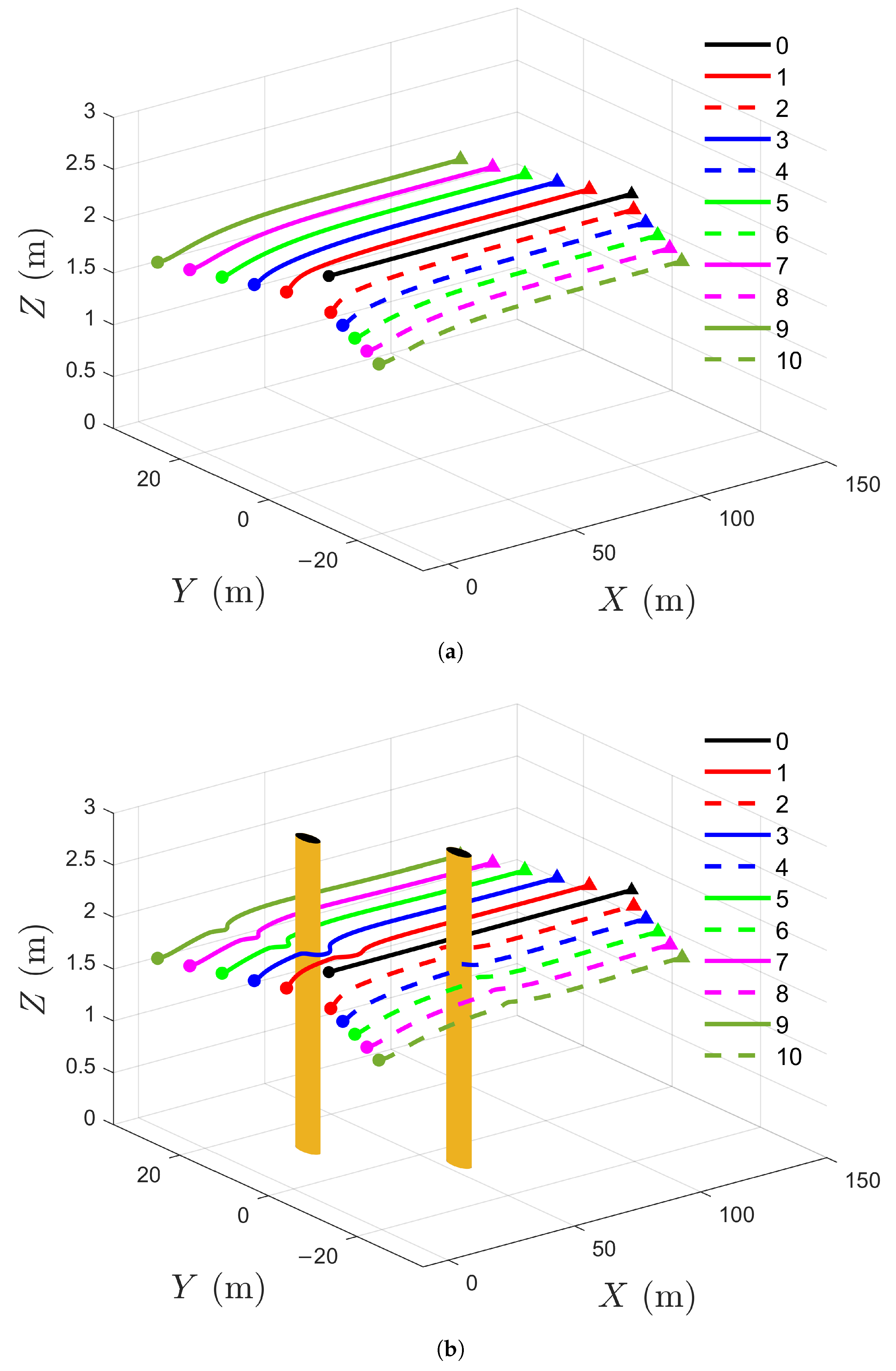
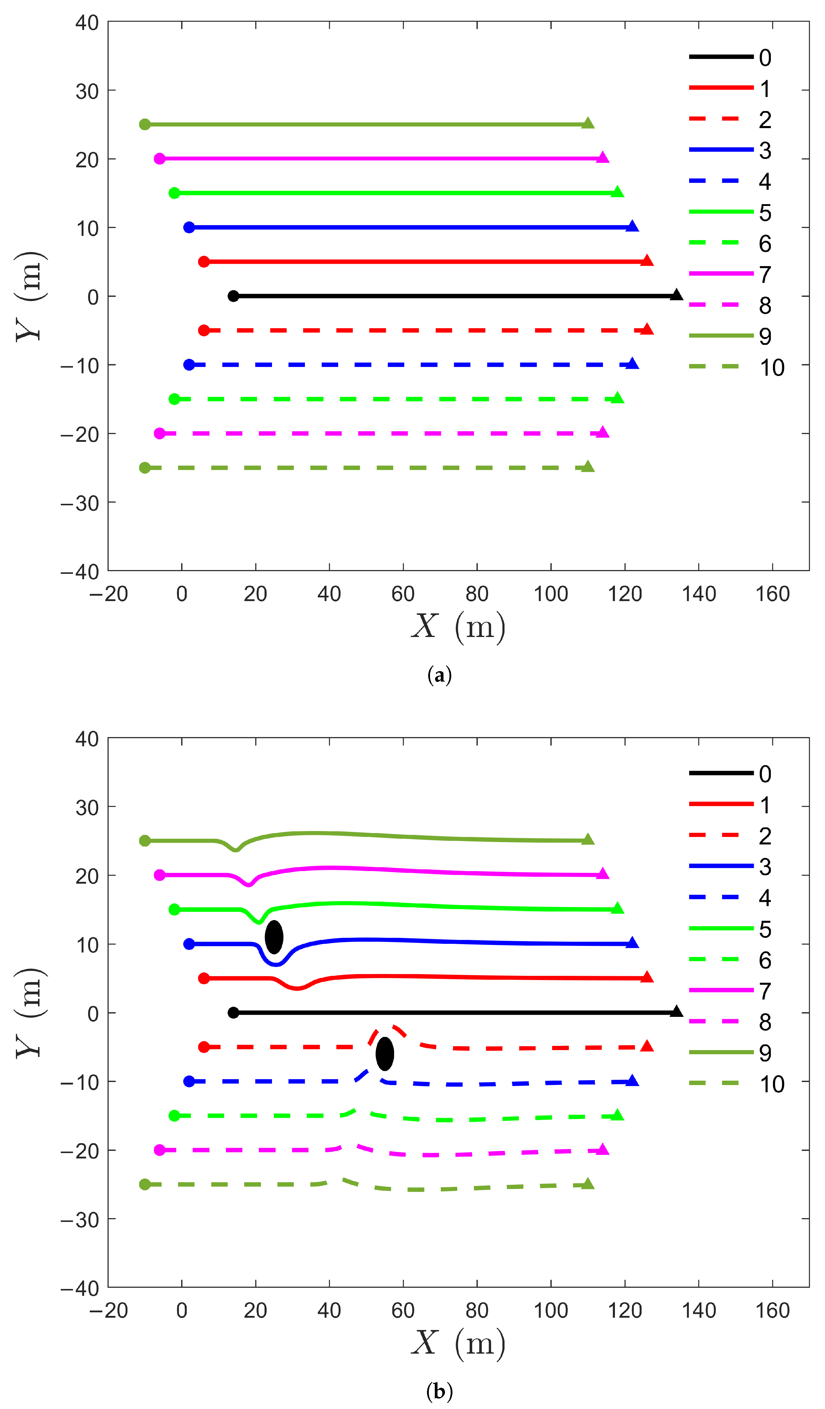
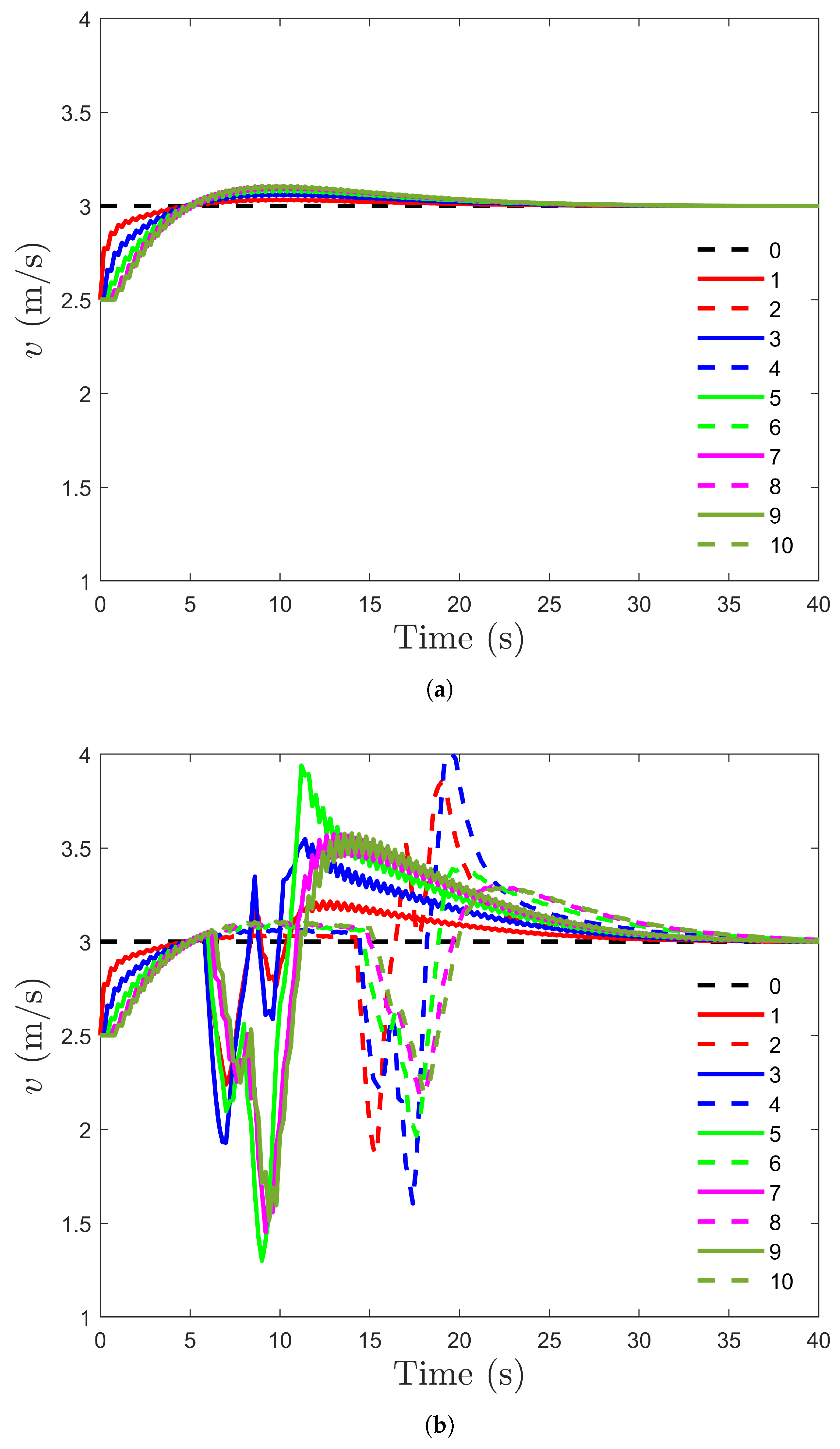
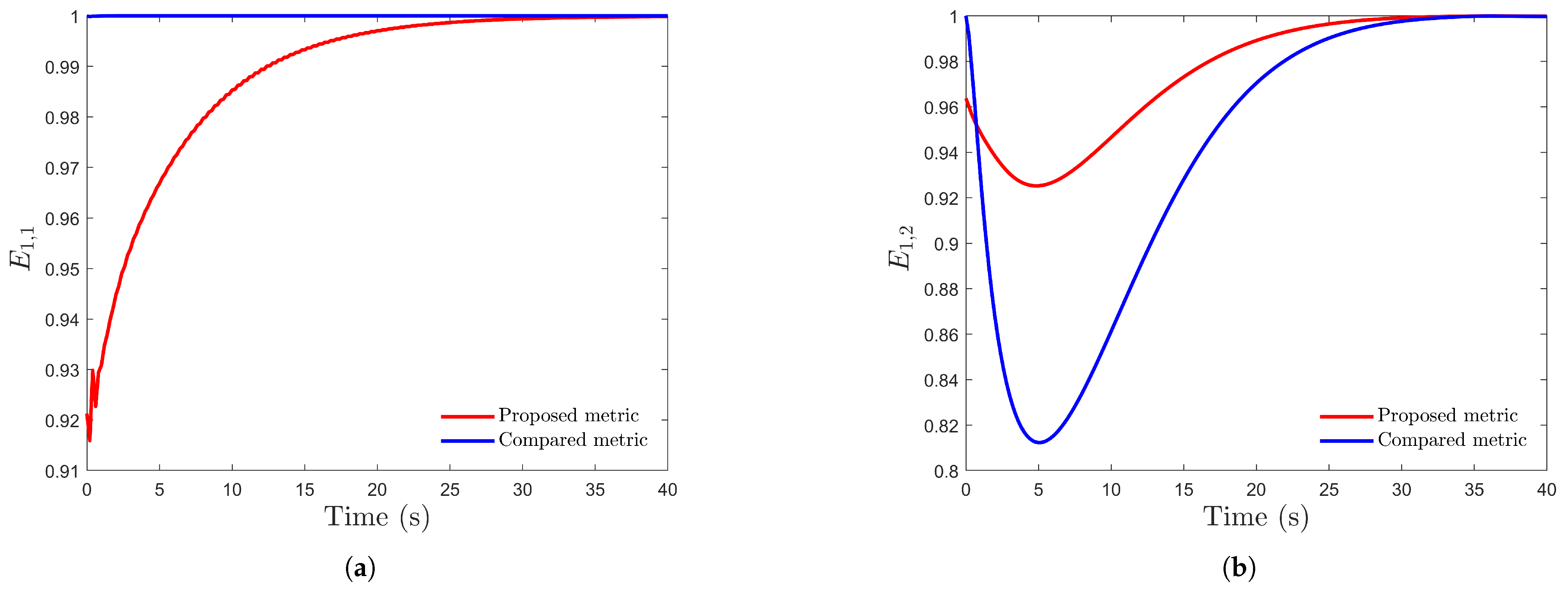
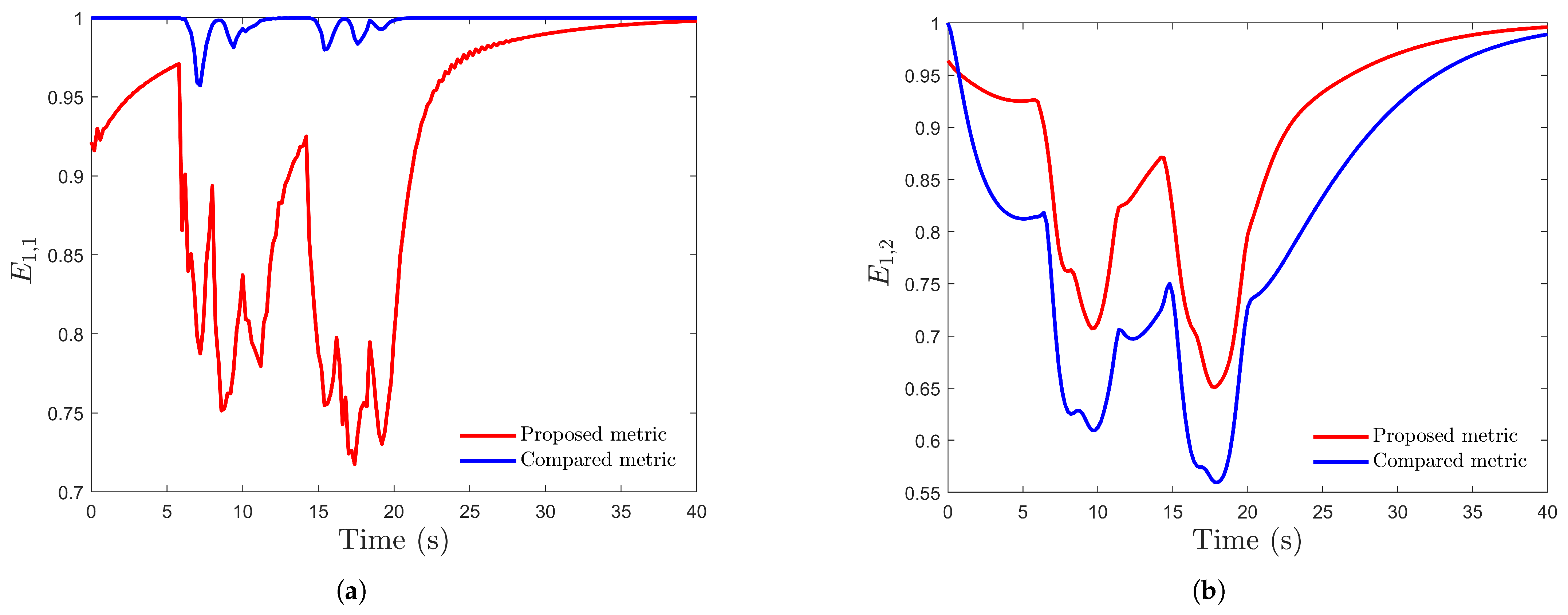
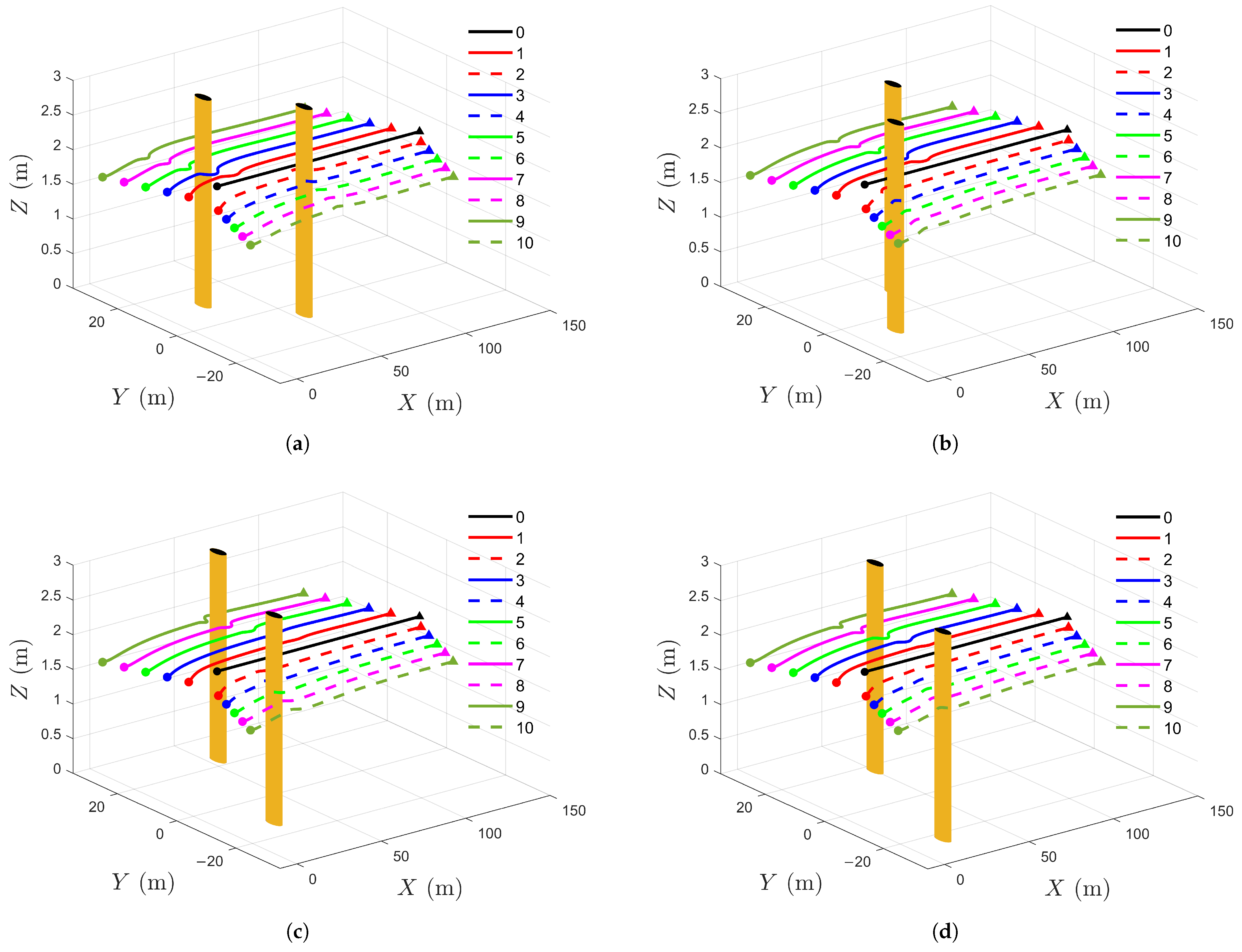
5.1. Formation Control for UAVs Without and with Obstacles

To validate the effectiveness of the formation control algorithm without and with obstacles, we select a tracked UAV (0) and ten tracking UAVs ($1,2,\dots ,10$) in the simulation. The communication topology is illustrated in Figure 1.

The initial state of the tracked UAV is designed as ${[14,0,2,3,0,0]}^T$, and it flies at a constant velocity ${[3,0,0]}^T$. The initial state of ten tracking UAVs, along with the relative state of UAV i concerning the tracked UAV, are shown in

Table 1. Initial state and desired relative state.

ID	Initial State	Desired Relative State
1	${[6,5,1.8,2.5,0,0]}^T$	${[-8,5,0,0,0,0]}^T$
2	${[6,-5,1.8,2.5,0,0]}^T$	${[-8,-5,0,0,0,0]}^T$
3	${[2,10,1.8,2.5,0,0]}^T$	${[-12,10,0,0,0,0]}^T$
4	${[2,-10,1.8,2.5,0,0]}^T$	${[-12,-10,0,0,0,0]}^T$
5	${[-2,15,1.8,2.5,0,0]}^T$	${[-16,15,0,0,0,0]}^T$
6	${[-2,-15,1.8,2.5,0,0]}^T$	${[-16,-15,0,0,0,0]}^T$
7	${[-6,20,1.8,2.5,0,0]}^T$	${[-20,20,0,0,0,0]}^T$
8	${[-6,-20,1.8,2.5,0,0]}^T$	${[-20,-20,0,0,0,0]}^T$
9	${[-10,25,1.8,2.5,0,0]}^T$	${[-24,25,0,0,0,0]}^T$
10	${[-10,-25,1.8,2.5,0,0]}^T$	${[-24,-25,0,0,0,0]}^T$

. In addition, simulation parameters are designed as shown in

Table 2. Simulation parameters.

Parameter	Value
Weighting coefficient ${\lambda }_{i,1}$	100
Prediction horizon $N_p$	5
Sampling period $\mathsf{\Delta }T$ (s)	$0.2$
Velocity range $\left[V_{min},V_{max}\right]$ (m/s)	$[1,4]$
Height range $\left[{\mathsf{\Xi }}_{min},{\mathsf{\Xi }}_{max}\right]$ (m)	$[1.5,2.5]$
Control input range $\left[U_{min},U_{max}\right]$ $\left({\mathrm{m}/\mathrm{s}}^2\right)$	$[-1.5,1.5]$
Safety distances $d_{\mathrm{c},\mathrm{saf}}$ (m) and $d_{\mathrm{o},\mathrm{saf}}$ (m)	1.2, 2.5
UAV detection range $d_{i,\det }$ (m)	4
Channel’s power gain $\rho$ (dB)	−20
Noise power ${\sigma }_{ij}^2$ (dBm)	−80
Communication bandwidth $B_{ij}$ (MHz)	1
Transmitted power P (dBm)	10

.

Figure 2a displays the 3D formation trajectories of UAVs without obstacles, while Figure 2b shows the 3D formation trajectories of UAVs with obstacles. In Figure 2a, the UAVs do not implement the obstacle avoidance strategy during flight because no obstacles are detected. In Figure 2b, the UAVs detect the obstacle and actively adjust their paths using the obstacle avoidance strategy, resulting in significant fluctuations in their trajectories.

Figure 3a displays the 2D formation trajectories of UAVs without obstacles, ensuring that the UAVs maintain a stable formation in the absence of obstacles. In contrast, Figure 3b shows the 2D formation trajectories of UAVs with obstacles, indicating that the proposed strategy allows the tracking UAVs to return to their desired relative positions after avoiding obstacles. Specifically, UAV 3 and UAV 5 take approximately 0.6 s and 1.2 s to avoid the first obstacle. In addition, UAV 2 and UAV 4 take approximately 1.2 s to avoid the second obstacle.

Figure 4a presents the flight velocities of UAVs without obstacles, while Figure 4b shows the flight velocities of UAVs with obstacles. From Figure 4a,b, it is clear that the velocities of tracking UAVs remain within the specified constraints. In addition, as can be seen in Figure 4b, the velocities of UAVs tend to be consistent in the initial stage, approaching the flight velocity of the tracked UAV. However, due to the detection of obstacles during the flight, the velocities exhibit significant fluctuations and stabilize again after the second obstacle avoidance maneuver.

The swarm’s cooperative capability evaluation results without and with obstacles are shown in Figure 5. When UAVs fly in an environment without obstacles, metrics such as velocity consistency, position matching, and communication equilibrium gradually approach 1, while safety remains consistently at 1. When UAVs fly in the environment with obstacles, metrics such as velocity consistency, position matching, and communication equilibrium exhibit significant fluctuations during obstacle avoidance maneuvers, and then gradually approach 1 after the second obstacle avoidance maneuver. Additionally, since UAVs implement obstacle avoidance strategies upon detecting obstacles, safety remains consistently at 1. These proposed metrics reflect the dynamic changes during swarm flight and demonstrate the applicability of the metrics design.

To validate the advantages of the swarm coordination evaluation metrics proposed in this paper, we conduct a comparative analysis with existing velocity consistency and position matching metrics that do not account for the state of the tracked UAV. The compared metrics are shown below:

$$\begin{array}{c}\hfill {\tilde{E}}_{1,1}\left(k\right)={\displaystyle \frac{1}{M}}\sum _{i=1}^M{\displaystyle \frac{1}{N_i}}\sum _{j\in {\mathcal{N}}_i}{\displaystyle \frac{v_i\left(k\right)·v_j\left(k\right)}{∥v_i\left(k\right)∥\parallel v_j\left(k\right)\parallel }}\end{array}$$

(23)

$$\begin{array}{c}\hfill {\tilde{E}}_{1,2}\left(k\right)={\displaystyle \frac{1}{M}}\sum _{i=1}^{M}exp\left(-{\displaystyle \frac{1}{N_i}}\sum _{j\in {\mathcal{N}}_i}∥p_i\left(k\right)-p_{ir}-p_j\left(k\right)+p_{jr}∥\right)\end{array}$$

(24)

where (23) is used to judge whether the velocity directions of UAVs are aligned. If the velocity direction tends to be the same, the value approaches 1. In addition, (24) is used to judge whether the UAVs maintain a desired formation shape during movement. If the relative position deviation between UAVs is slight, the value is close to 1.

In Figure 6 and Figure 7, since the tracking UAVs have the same initial velocities and their relative position errors match the expected values, the compared metrics equal 1. However, these metrics overlook the influence of the tracked UAV on the swarm’s collective motion, resulting in incomplete assessment results. Consequently, the metrics values should not equal 1 at the initial moment. Additionally, the velocity consistency metric evaluates only directional alignment while disregarding velocity magnitude consistency, leading to imprecise assessments. In contrast, the coordination metrics presented in this paper consider the state of the tracked UAV and velocity magnitude, ensuring evaluation results of coordination that better reflect actual conditions.

5.2. Formation Control for UAVs in Different Scenarios

To verify the effectiveness of the proposed method in different scenarios,

Table 3. The coordinates of obstacles in different scenarios.

Scenario	Coordinate for Obstacle 1	Coordinate for Obstacle 2
1	${[25,11]}^T$	${[55,-6]}^T$
2	${[20,-7]}^T$	${[50,11]}^T$
3	${[25,-13]}^T$	${[55,23]}^T$
4	${[20,-23]}^T$	${[50,17]}^T$

shows the coordinates of the four groups of obstacles.

The 3D and 2D formation trajectories of UAVs in different scenarios are demonstrated in Figure 8 and Figure 9, respectively. It can be seen that the UAVs successfully avoid obstacles in four scenarios, verifying the effectiveness of the proposed method.

The swarm’s cooperative capability evaluation results in different scenarios are shown in Figure 10. In different scenarios, velocity consistency, position matching, and communication equilibrium exhibit significant fluctuations during obstacle avoidance maneuvers, and then gradually approach 1 after the second obstacle avoidance maneuver. Additionally, since UAVs implement obstacle avoidance strategies upon detecting obstacles, safety remains consistently at 1 in different scenarios.

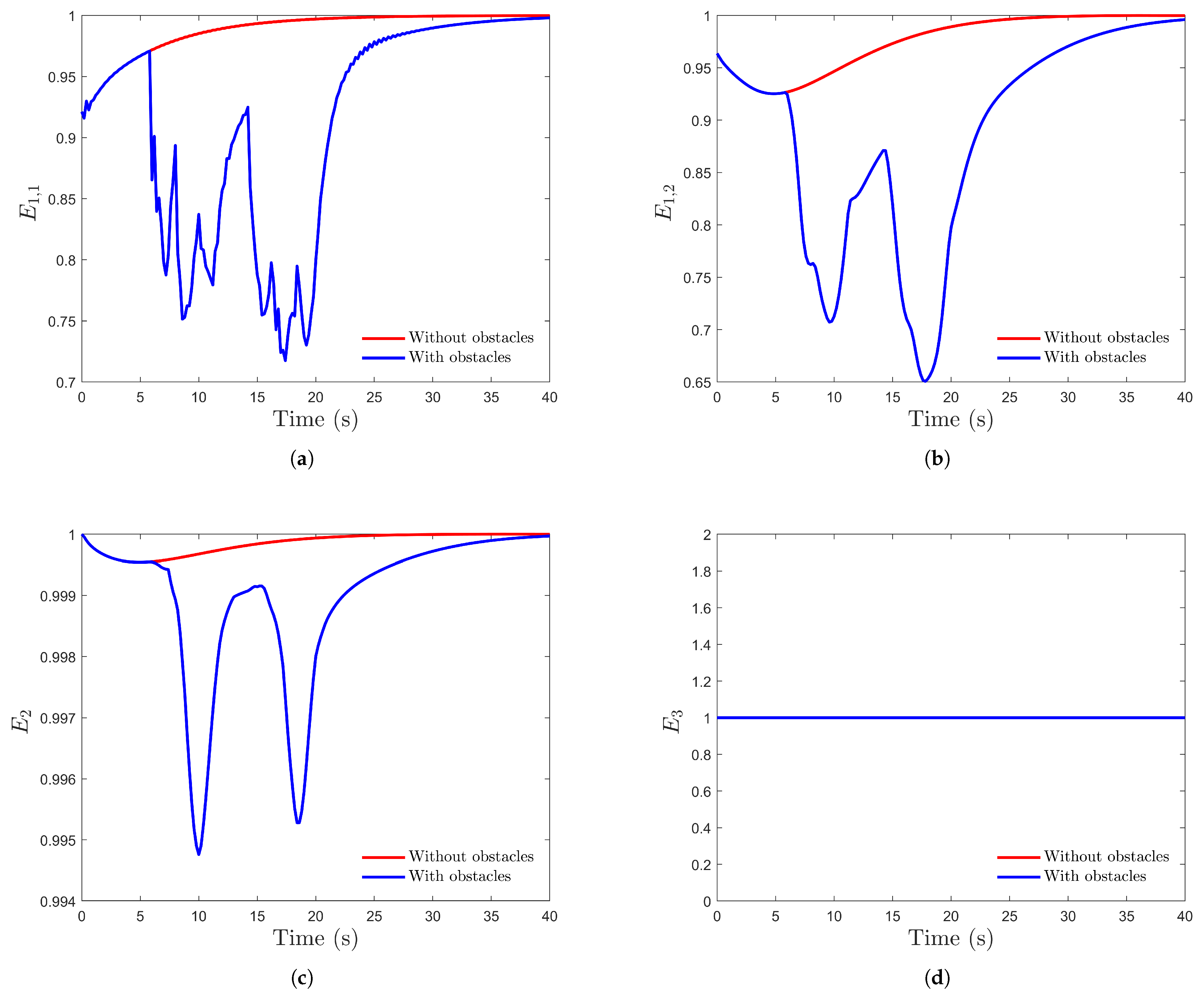
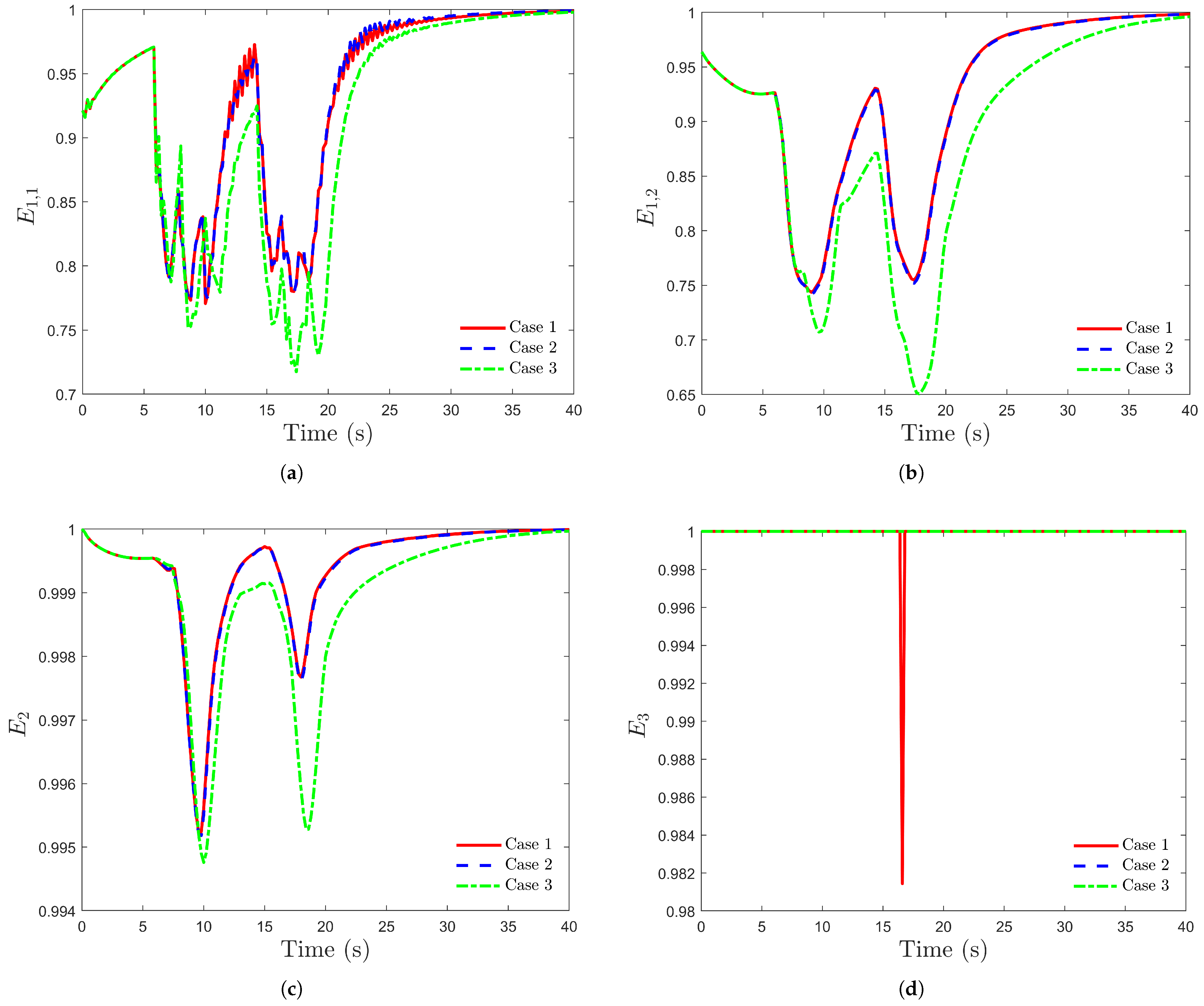
5.3. Cooperative Capability Evaluation Results Under Different Weighting Coefficients

Although the method proposed in Section 5.1 achieves obstacle avoidance when ${\lambda }_{i,1}=100$, the empirically selected weight significantly decreases swarm coordination and communication equilibrium during obstacle avoidance. Therefore, based on the established evaluation metrics, we obtained a weight of ${\lambda }_{i,1}=43$, which ensures swarm safety $E_3\left(k\right)=1$ while having a minor impact on the other evaluation metrics. Then, we compared it with several other weighting coefficients. The three groups of weighting coefficients are shown in

Table 4. The weighting coefficient in the cost function.

Case	${\mathit{\lambda }}_{\mathit{i},1}$
1	42
2	43
3	100

.

The swarm’s cooperative capability evaluation results under different weighting coefficients are shown in Figure 11. Compared with Case 1, Case 2 ensures that the safety of UAVs remains at 1 throughout the flight. Additionally, compared with Case 3, Case 2 maintains safety at 1 while mitigating the excessive decline in velocity consistency, position matching, and communication equilibrium caused by excessively high obstacle avoidance weight. This validates the effectiveness of adjusting the obstacle avoidance weight based on evaluation metrics, ensuring a proper balance between safety and other cooperative capability metrics.

6. Conclusions

In this paper, we propose a formation control algorithm based on synchronized DMPC. The algorithm integrates formation error and obstacle avoidance into a distributed optimization framework, ensuring optimal control input for each UAV while satisfying multiple constraints. To comprehensively evaluate the cooperative capability of the swarm, we adopt coordination, communication equilibrium, and safety as key evaluation metrics, effectively reflecting the swarm’s cooperative capability. Finally, simulation results show the effectiveness of the designed method.

References

1. Luo, Q.; Luan, T.H.; Shi, W.; Fan, P. Edge Computing Enabled Energy-Efficient Multi-UAV Cooperative Target Search. IEEE Trans. Veh. Technol. 2023, 72, 7757–7771. [Google Scholar] [CrossRef]
2. Dai, J.; Pu, W.; Yan, J.; Shi, Q.; Liu, H. Multi-UAV Collaborative Trajectory Optimization for Asynchronous 3-D Passive Multitarget Tracking. IEEE Trans. Geosci. Remote Sens. 2023, 61, 1–16. [Google Scholar] [CrossRef]
3. Sun, L.; Wang, J.; Wang, J.; Lin, L.; Gen, M. Efficient Joint Deployment of Multi-UAVs for Target Tracking in Traffic Big Data. IEEE Trans. Intell. Transp. Syst. 2024, 25, 7780–7791. [Google Scholar] [CrossRef]
4. Gu, J.; Su, T.; Wang, Q.; Du, X.; Guizani, M. Multiple Moving Targets Surveillance Based on a Cooperative Network for Multi-UAV. IEEE Commun. Mag. 2018, 56, 82–89. [Google Scholar] [CrossRef]
5. Yu, Y.; Guo, J.; Ahn, C.K.; Xiang, Z. Neural Adaptive Distributed Formation Control of Nonlinear Multi-UAVs With Unmodeled Dynamics. IEEE Trans. Neural Netw. Learn. Syst. 2022, 34, 9555–9561. [Google Scholar] [CrossRef]
6. Ding, C.; Zhang, Z.; Zhang, J. Dynamics Event-Triggered-Based Time-Varying Bearing Formation Control for UAVs. Drones 2024, 8, 185. [Google Scholar] [CrossRef]
7. Zheng, R.; Lyu, Y. Nonlinear tight formation control of multiple UAVs based on model predictive control. Def. Technol. 2023, 25, 69–75. [Google Scholar] [CrossRef]
8. Zhan, J.; Jiang, Z.P.; Wang, Y.; Li, X. Distributed Model Predictive Consensus With Self-Triggered Mechanism in General Linear Multiagent Systems. IEEE Trans. Ind. Inf. 2019, 15, 3987–3997. [Google Scholar] [CrossRef]
9. Wang, J.; Li, S. Distributed Model Predictive Control for Consensus of Multi-Agent Systems With Connectivity Maintenance. IEEE Trans. Circuits Syst. I Regul. Pap. 2023, 71, 1299–1310. [Google Scholar] [CrossRef]
10. Chen, Q.; Jin, Y.; Wang, T.; Wang, Y.; Yan, T.; Long, Y. UAV Formation Control Under Communication Constraints Based on Distributed Model Predictive Control. IEEE Access 2022, 10, 126494–126507. [Google Scholar] [CrossRef]
11. Liu, S.S.; Ge, M.F.; Ding, T.F.; Liu, Z.W.; Dong, X.G.; Liang, C.D. Distributed Sensor-Tolerant MPC for Formation Tracking of Networked Multicopters With Input/State Constraints. IEEE Trans. Circuits Syst. II Express Briefs 2023, 70, 4429–4433. [Google Scholar] [CrossRef]
12. Yuan, Q.; Li, X. Distributed Model Predictive Formation Control for a Group of UAVs With Spatial Kinematics and Unidirectional Data Transmissions. IEEE Trans. Netw. Sci. Eng. 2023, 10, 3209–3222. [Google Scholar] [CrossRef]
13. Xu, T.; Liu, J.; Zhang, Z.; Chen, G.; Cui, D.; Li, H. Distributed MPC for Trajectory Tracking and Formation Control of Multi-UAVs With Leader-Follower Structure. IEEE Access 2023, 11, 128762–128773. [Google Scholar] [CrossRef]
14. Cai, Z.; Wang, L.; Zhao, J.; Wu, K.; Wang, Y. Virtual target guidance-based distributed model predictive control for formation control of multiple UAVs. Chin. J. Aeronaut. 2020, 33, 1037–1056. [Google Scholar] [CrossRef]
15. Zhang, B.; Sun, X.; Liu, S.; Deng, X. Adaptive differential evolution-based distributed model predictive control for multi-UAV formation flight. Int. J. Aeronaut. Space Sci. 2020, 21, 538–548. [Google Scholar] [CrossRef]
16. Chen, G.; Zhao, C.; Gong, H.; Zhang, S.; Wang, X. Formation Transformation Based on Improved Genetic Algorithm and Distributed Model Predictive Control. Drones 2023, 7, 527. [Google Scholar] [CrossRef]
17. He, Y.; Shi, X.; Lu, J.; Zhao, C.; Zhao, G. Grouping Formation and Obstacle Avoidance Control of UAV Swarm Based on Synchronous DMPC. Int. J. Aerosp. Eng. 2024, 2024, 4934194. [Google Scholar] [CrossRef]
18. Du, Z.; Zhang, H.; Wang, Z.; Yan, H. Model Predictive Formation Tracking-Containment Control for Multi-UAVs With Obstacle Avoidance. IEEE Trans. Syst. Man Cybern. Syst. 2024, 54, 3404–3414. [Google Scholar] [CrossRef]
19. Vásárhelyi, G.; Virágh, C.; Somorjai, G.; Nepusz, T.; Eiben, A.E.; Vicsek, T. Optimized flocking of autonomous drones in confined environments. Sci. Robot. 2018, 3, eaat3536. [Google Scholar] [CrossRef]
20. Cofta, P.; Ledziński, D.; Śmigiel, S.; Gackowska, M. Cross-entropy as a metric for the robustness of drone swarms. Entropy 2020, 22, 597. [Google Scholar] [CrossRef]
21. Bahaidarah, M.; Rekabi-Bana, F.; Marjanovic, O.; Arvin, F. Swarm flocking using optimisation for a self-organised collective motion. Swarm Evol. Comput. 2024, 86, 101491. [Google Scholar] [CrossRef]
22. Zhang, X.; Wang, Y.; Ding, W.; Wang, Q.; Zhang, Z.; Jia, J. Bio-Inspired Fission–Fusion Control and Planning of Unmanned Aerial Vehicles Swarm Systems via Reinforcement Learning. Appl. Sci. 2024, 14, 1192. [Google Scholar] [CrossRef]
23. Rodríguez, I.; Rubio, D.; Rubio, F. Complexity of adaptive testing in scenarios defined extensionally. Front. Comput. Sci. 2023, 17, 173206. [Google Scholar] [CrossRef]
Figure 1. Communication topology of UAVs.
Drones 09 00366 g001
Figure 2. Three-dimensional formation trajectories without and with obstacles: (a) Three-dimensional formation trajectories without obstacles. (b) Three-dimensional formation trajectories with obstacles.
Drones 09 00366 g002
Figure 3. Two-dimensional formation trajectories without and with obstacles: (a) Two-dimensional formation trajectories without obstacles. (b) Two-dimensional formation trajectories with obstacles.
Drones 09 00366 g003
Figure 4. The flight velocities without and with obstacles: (a) The flight velocities without obstacles. (b) The flight velocities with obstacles.
Drones 09 00366 g004
Figure 5. Swarm’s cooperative capability evaluation results without and with obstacles: (a) Velocity consistency of swarm. (b) Position matching of swarm. (c) Communication equilibrium of swarm. (d) Safety of swarm.
Drones 09 00366 g005
Figure 6. Comparison results of the swarm coordination evaluation metrics without obstacles: (a) Velocity consistency of the swarm. (b) Position matching of the swarm.
Drones 09 00366 g006
Figure 7. Comparison results of the swarm coordination evaluation metrics with obstacles: (a) Velocity consistency of the swarm. (b) Position matching of the swarm.
Drones 09 00366 g007
Figure 8. Three-dimensional formation trajectories in different scenarios: (a) Three-dimensional formation trajectories in scenario 1. (b) Three-dimensional formation trajectories in scenario 2. (c) Three-dimensional formation trajectories in scenario 3. (d) Three-dimensional formation trajectories in scenario 4.
Drones 09 00366 g008
Figure 9. Two-dimensional formation trajectories in different scenarios: (a) Two-dimensional formation trajectories in scenario 1. (b) Two-dimensional formation trajectories in scenario 2. (c) Two-dimensional formation trajectories in scenario 3. (d) Two-dimensional formation trajectories in scenario 4.
Drones 09 00366 g009
Figure 10. Swarm’s cooperative capability evaluation results in different scenarios: (a) Velocity consistency of swarm. (b) Position matching of swarm. (c) Communication equilibrium of swarm. (d) Safety of swarm.
Drones 09 00366 g010
Figure 11. Swarm’s cooperative capability evaluation results under different weighting coefficients: (a) Velocity consistency of swarm. (b) Position matching of swarm. (c) Communication equilibrium of swarm. (d) Safety of swarm.
Drones 09 00366 g011