Article

Identification of Salt Marsh Vegetation in the Yellow River Delta Using UAV Multispectral Imagery and Deep Learning

1
Academician Workstation for Big Data in Ecology and Environment, Environment Research Institute, Shandong University, Qingdao 266003, China
2
Shandong Yellow River Delta National Nature Reserve Management Committee, Dongying 257091, China
3
National Marine Environmental Monitoring Center, Dalian 116023, China
4
School of Marine Science and Technology, Northwestern Polytechnical University, Xi’an 710072, China
5
Institute of Ecology and Biodiversity, School of Life Sciences, Shandong University, Qingdao 266237, China
6
Center for Geodata and Analysis, Faculty of Geographical Science, Beijing Normal University, Beijing 100875, China
*
Author to whom correspondence should be addressed.
Drones 2025, 9(4), 235; https://doi.org/10.3390/drones9040235
Submission received: 10 February 2025 / Revised: 14 March 2025 / Accepted: 21 March 2025 / Published: 23 March 2025

Abstract

:
Salt marsh ecosystems play a critical role in coastal protection, carbon sequestration, and biodiversity preservation. However, they are increasingly threatened by climate change and anthropogenic activities, necessitating precise vegetation mapping for effective conservation. This study investigated the effectiveness of spectral features and machine learning models in separating typical salt marsh vegetation types in the Yellow River Delta using uncrewed aerial vehicle (UAV)-derived multispectral imagery. The results revealed that the Normalized Difference Vegetation Index (NDVI), Green Normalized Difference Vegetation Index (GNDVI), and Optimized Soil Adjusted Vegetation Index (OSAVI) were pivotal in differentiating vegetation types, compared with spectral reflectance at individual bands. Among the evaluated models, U-Net achieved the highest overall accuracy (94.05%), followed by SegNet (93.26%). However, the U-Net model produced overly distinct and abrupt boundaries between vegetation types, lacking the natural transitions found in real vegetation distributions. In contrast, the SegNet model excelled in boundary handling, better capturing the natural transitions between vegetation types. Both deep learning models outperformed Random Forest (83.74%) and Extreme Gradient Boosting (83.34%). This study highlights the advantages of deep learning models for precise salt marsh vegetation mapping and their potential in ecological monitoring and conservation efforts.

1. Introduction

Salt marsh ecosystems represent critical ecological transition zones connecting land and ocean, formed by the alternating interactions of terrestrial rivers and marine tides [1,2,3]. As primary producers within intertidal systems, salt marshes fulfill critical ecological functions, including mitigating storm surges, enhancing sedimentation and coastal protection, purifying seawater, and serving as habitats for diverse wildlife [4,5,6]. In recent years, salt marsh ecosystems have garnered significant attention due to their remarkable ‘blue carbon’ sequestration capabilities [7]. However, salt marshes are increasingly threatened by the dual pressures of global climate change and human activities [8,9]. Some research reported that global salt marshes have decreased by 25–50% [10]. Therefore, efficiently acquiring spatial distribution and vegetation composition information of coastal salt marshes is essential for ecosystem conservation.
Remote sensing technology offers a powerful tool for large-scale monitoring of salt marsh vegetation. With the rapid development of sensors, satellite-based land surface observation has evolved from medium-resolution to high-resolution imaging and from single-source to multi-source data integration. Early research by Leahy et al. (2005) used multi-temporal Landsat satellite images to detect long-term changes in wetlands in Ontario, Canada [11]. Subsequently, the introduction of high-quality Sentinel-1/2 significantly improved the classification accuracy of coastal ecosystems [12]. Moreover, GF-1 and GF-6 imagery were also utilized for high-precision mapping of wetlands in the Sanjiang National Nature Reserve, demonstrating the advantages of high-resolution remote sensing data in the wetland classification [13]. However, traditional satellite remote sensing still faces challenges in fine-scale salt marsh vegetation identification due to the mixed distribution of salt-tolerant grass communities [14].
Uncrewed aerial vehicle (UAV) remote sensing is a popular means to carry out centimeter-resolution, flexible, and low-cost monitoring of ecosystems, making it an important approach for accurate classification of salt marsh vegetation [15,16,17]. For instance, high-resolution UAV imagery has been successfully applied to quantify the fine-scale spatial patterns of invasive plant species [18] and to classify and compare the composition and structure of vegetation in tidal flat areas [14]. Moreover, the integration of UAV imagery with deep learning techniques (e.g., CNN+OBIA methods) has been shown to effectively identify plant species in complex vegetation communities [19]. Additionally, studies have demonstrated that centimeter-level multispectral UAV imagery can achieve fine-scale, species-level classification of peatland vegetation, particularly during the early or peak growing seasons, offering significant value for monitoring restoration projects [20]. However, despite the widespread usage of UAV data for vegetation classification and mapping, there is still a lack of systematic analysis regarding the spectral difference of salt marsh vegetation types and the relative importance of vegetation indices in distinguishing them.
The evolution of machine learning has significantly advanced the accuracy and efficiency of vegetation recognition from remote sensing images. Initial approaches relied primarily on traditional methods such as Maximum Likelihood Classification [21] and Support Vector Machines [22]. With the advancement of artificial intelligence technologies, ensemble learning algorithms, particularly Random Forest (RF) [23] and Extreme Gradient Boosting Tree (XGBoost) [24], emerged as powerful tools for vegetation classification. A study combining Random Forest algorithms with diverse remote sensing data sources, including quad polarimetric airborne SAR, elevation data, and Landsat images, achieved remarkable performance in coastal wetland classification, with overall accuracy surpassing 85.75%, demonstrating the robustness of ensemble learning approaches [25]. In recent years, deep learning methods have demonstrated significant advantages in wetland classification based on remote sensing images. One study employed the U-Net model to map salt marsh distributions in South Carolina, achieving an impressive OA of 90% [26]. In a similar vein, another research applied an enhanced U-Net model to classify wetlands in Vietnam’s Tien Yen Estuary, attaining 85% classification accuracy [27].
This study aims to explore the feasibility of combining UAV images and machine learning in multi-species accurate classification for typical salt marsh vegetation. Specifically, we plan to (1) analyze the characteristic gaps of spectral features and vegetation indices across different salt marsh vegetation types for elaborately understanding their potential for accurate mapping and (2) compare the classification performance of machine learning (e.g., RF and XGBoost) and deep learning (e.g., U-Net and SegNet) models in fine-scale identification of salt marsh vegetation. We hope to enhance the precision and efficiency of salt marsh vegetation classification and support sustainable coastal ecosystem management with the results of this study.

2. Materials and Methods
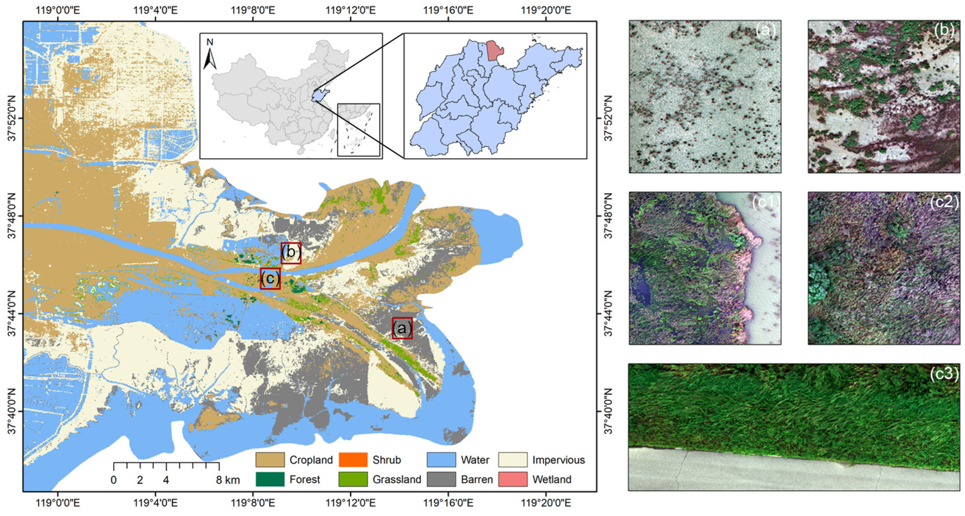
2.1. Study Area

The Yellow River Delta (119°06′–119°18′ E, 37°40′–37°52′ N) is located in the Shandong Province of China and features a warm temperate continental monsoon climate, with an average annual temperature of 11.9 °C and precipitation of 590.9 mm. It covers a total area of approximately 5450 km2, with the study flights covering 0.065 km2. It is one of the highest sediment-producing regions globally and represents China’s largest and youngest salt marsh ecosystem [28,29]. The typical vegetation community in this region includes Suaeda salsa, Phragmites australis, and Tamarix chinensis [30,31]. Suaeda salsa, with its exceptional salt tolerance, demonstrates significant potential for ecological restoration in high-salinity soils, contributing to soil nutrient accumulation and land amelioration [32]. Phragmites australis, a widely distributed perennial herb, serves dual ecological functions: regulating soil moisture and salinity while providing crucial habitats for migratory birds [33]. Tamarix chinensis, as a salt-tolerant woody species, represents an ideal choice for ecological restoration in saline-alkali lands [34].

2.2. Data Acquisition and Preprocessing

Images were collected using a DJI Phantom 4 Multispectral (P4M) drone on 14–15 September 2024 across five representative sampling sites characterized by distinct vegetation types and coverage patterns (Figure 1). The UAV flights were conducted between 10:00 AM and 4:00 PM under clear sky conditions with minimal cloud cover (<10%) and light wind speeds (<5 m/s) to ensure optimal and consistent lighting conditions for spectral imagery collection. The UAV was flown at an altitude of 40 m, resulting in a ground sampling distance (GSD) of approximately 2 cm/pixel. To balance image resolution, flight efficiency, and battery constraints, the flight parameters were set to a speed of 10 m·s⁻¹ with 20% forward overlap and 30% side overlap, covering a total area of 0.065 km2. While higher overlap values are generally recommended for complex wetland environments, preliminary tests confirmed that these settings were sufficient to generate high-quality orthomosaics and reliable vegetation classification results. Additionally, the relatively homogeneous distribution of dominant vegetation types in the study area reduced the necessity for higher overlap.
The P4M system integrates six CMOS sensors: one panchromatic/visible light camera and five multispectral cameras with 2 million effective pixels. The multispectral array captures information across five spectral bands: blue (450 ± 16 nm), green (560 ± 16 nm), red (650 ± 16 nm), red-edge (730 ± 16 nm), and near-infrared (840 ± 26 nm). The integration of Real-Time Kinematic (RTK) technology enables centimeter-level positioning accuracy and enhances the geometric precision of the resulting orthophotos.
Image processing was performed using Agisoft PhotoScan software, which employs sophisticated fusion algorithms to optimize matching accuracy in overlapping regions. The workflow included image alignment, dense point cloud generation, Digital Elevation Model (DEM) construction, and orthophoto generation, ultimately producing the multispectral orthophoto of the study area (Figure 1). The spatial resolution of the generated multispectral orthophoto is approximately 2 cm.

2.3. Construction of the Sample Dataset

To establish a comprehensive and representative dataset of salt marsh vegetation, we implemented a rigorous sampling strategy based on two key criteria: (1) ensuring coverage of five typical salt marsh vegetation types to represent the ecosystem’s composition fully (Table 1) and (2) varying vegetation coverage densities to capture diverse spectral signatures for elevating model generalization capability. Visual interpretation was then conducted for sampling based on field survey results, incorporating spatial distribution, texture characteristics, and spectral features of vegetation types. A total of 5 field visits were conducted across the study area, with sampling sites selected to represent typical salt marsh species and varying vegetation coverage densities within the Yellow River Delta. Following the above stringent sample selection criteria, we constructed a multi-class pixel dataset with detailed distribution and proportion of pixels across different vegetation classes, as shown in Table 2. In order to ensure robust model training, the dataset was split into 80% for training and 20% for validation.

2.4. Vegetation Indices

To provide a comprehensive analysis of the spectral characteristics of salt marsh vegetation, this study extracted seven representative vegetation indices from multispectral UAV images, including the Normalized Difference Vegetation Index (NDVI) [35], Green Normalized Difference Vegetation Index (GNDVI) [36], Rededge Normalized Difference (NDRE) [37], Leaf Chlorophyll Index (LCI) [38], Optimized Soil Adjusted Vegetation Index (OSAVI) [39], Green Chromatic Coordinate (GCC) [40], and Coastal Redness Vegetation Index (CRVI) [41].
NDVI is effective in characterizing vegetation vigor and coverage by calculating the difference in reflectance between the red and near-infrared bands. GNDVI and NDRE enhance sensitivity to variations in chlorophyll content by incorporating green and red-edge spectral signals, respectively. LCI is specifically designed to assess chlorophyll and nitrogen content at the leaf level, while OSAVI improves the accuracy of vegetation signal extraction by reducing soil background interference. GCC captures information about vegetation coverage within the visible spectrum. Based on the work of Zeng et al. (2022), the CRVI has been shown to be effective in identifying Suaeda salsa [41].

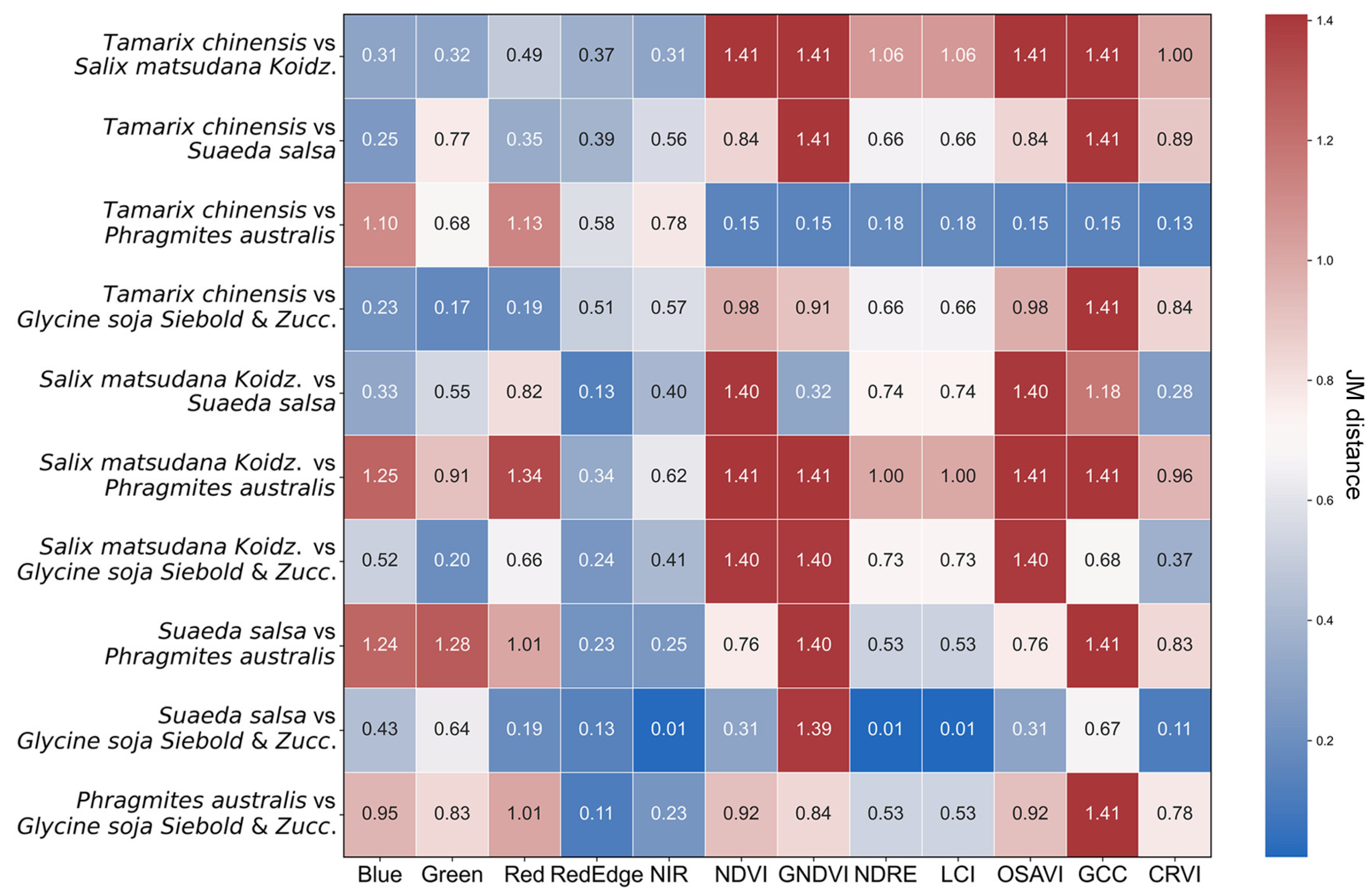
2.5. Jeffries–Matusita (JM) Distance

The Jeffries–Matusita (JM) distance was employed to evaluate the spectral separability of vegetation types and assess the discriminative capability of selected features [42,43]. The JM distance is a statistical metric that quantifies the distance between two probability distributions, with values ranging from 0 to 2. A higher JM distance indicates better separability between classes. This study calculated the JM distance for all pairwise combinations of vegetation types based on their spectral and vegetation index features.

2.6. Machine Learning Algorithms

2.6.1. Random Forest

Random forest (RF), an ensemble learning method, improves accuracy and robustness by constructing multiple decision trees and outputting the majority vote [44,45]. It is effective for handling high-dimensional data and is resistant to overfitting. Key parameters influencing performance are the number of trees and tree depth. In this study, 150 decision trees with a maximum depth of 20 were used to balance model performance and overfitting risk.

2.6.2. XGBoost

Extreme Gradient Boosting Tree (XGBoost), a powerful gradient boosting algorithm, combines multiple weak learners to construct an accurate and robust model [46]. It excels in handling high-dimensional data and capturing complex patterns. Its built-in regularization mechanisms further enhance performance by reducing overfitting. In this study, XGBoost was optimized for classification tasks with the following parameters: 100 decision trees, a maximum tree depth of 20, and a learning rate of 0.1. We implemented these traditional machine learning models using Python 3.10, leveraging the scikit-learn library for training, validation, and accuracy assessment.

2.7. Deep Learning Algorithms

2.7.1. U-Net

U-Net is a convolutional neural network (CNN) for image segmentation introduced by the University of Freiburg in 2015 [47]. Its encoder-decoder structure with skip connections helps preserve spatial resolution during upsampling. The encoder extracts features through convolution and pooling, while the decoder restores spatial resolution via upsampling, with skip connections refining segmentation boundaries [48,49].

2.7.2. SegNet

SegNet is a deep convolutional neural network for semantic segmentation. The architecture features an encoder-decoder structure, where the encoder extracts spatial features using convolution and pooling layers, and the decoder reconstructs segmentation maps by leveraging pooling indices from the encoder [50]. Unlike U-Net, SegNet restores resolution without transferring the entire feature map via concatenation, relying instead on pooling indices for efficient decoding [51].
In this study, UAV images were preprocessed for both U-Net and SegNet models in the same manner. Images were cropped into 256 × 256 pixel tiles to standardize input dimensions. Data augmentation techniques, including random rotation, flipping, and mirroring, were applied to enhance the feature space and improve model generalization. Both models were trained using the Adam optimizer [52] with a learning rate of 0.0001 and a weight decay coefficient of 0.0001. Training was conducted for 200 epochs, with each epoch comprising 10 batches. Both U-Net and SegNet were implemented using Python 3.10 and PyTorch 2.1.0.

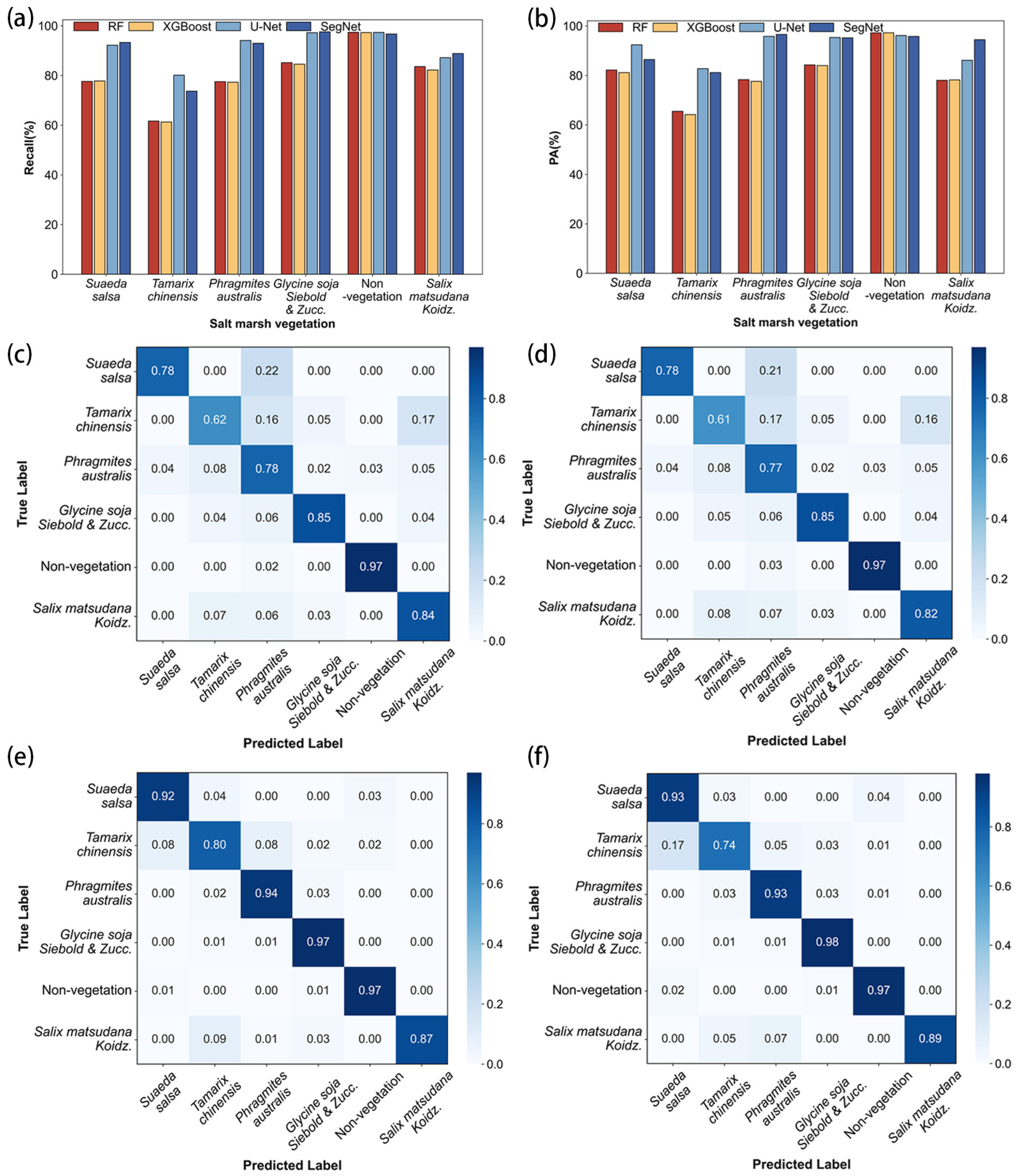
2.8. Accuracy Evaluation

This study employed a multidimensional accuracy evaluation approach to comprehensively assess the classification models’ performance. The evaluation framework includes the following metrics: (1) Confusion matrix visualization, which provides an intuitive representation of the correspondence between predicted results and actual classes; (2) Overall Accuracy (OA), which quantifies the model’s overall prediction accuracy across the entire dataset; (3) Kappa coefficient, which accounts for random agreement and serves as a more robust metric compared to traditional accuracy measures; (4) Producer’s Accuracy (PA) and Recall, which offer detailed evaluations of the model’s classification performance for both positive and negative samples; and (5) F1 score, a harmonic mean of precision and recall, which balances the model’s precision and recall capabilities.

3. Results

3.1. Spectral Characteristics and Divisibility Analysis of Wetland Vegetation Types

Spectral analysis showed a relatively higher gap in the red and green bands across the five investigated species (Figure 2a). Specifically, a greater difference identified in the near-infrared band could be effectively used to distinguish Phragmites australis and Suaeda salsa from the other three species, while a strong divisibility was detected in the blue and green band for Phragmites australis and Suaeda salsa. By means of the distinct spectral characteristics in the blue and red band, it is also likely to separate Tamarix chinensis from Salix matsudana Koidz. and Glycine soja Siebold & Zucc. However, there is a large spectral overlap between Salix matsudana Koidz. and Glycine soja Siebold & Zucc. in all five bands, making it hard to differentiate them.
Vegetation indices presented a better capability to identify the five targeted species than solely band values (Figure 2b). A very similar profile was found between NDVI and OSAVI and between NDRE and LCI, meaning identical potential for vegetation classification. Both GCC and CRVI displayed significant distances among five species, except for Salix matsudana Koidz. and Tamarix chinensis, which suggests wonderful potential to distinguish them. The values of chlorophyll-related indices (NDVI, GNDVI, OSAVI) were relatively lower for Phragmites australis and Suaeda salsa and were largely different from that of Glycine soja Siebold & Zucc. and Salix matsudana Koidz.
The JM distance analysis further demonstrated that vegetation indices generally provided strong discriminatory power for distinguishing salt marsh vegetation types (Figure 3). Consistent with Figure 2b, GNDVI, GCC, NDVI, and OSAVI exhibited similar classification potential, with JM distances exceeding 1.4 for most species pairs, particularly for Tamarix chinensis vs. Salix matsudana Koidz. and Salix matsudana Koidz. vs. Phragmites australis. In contrast, the red edge and near-infrared bands exhibited low JM distances (<0.5), indicating limited effectiveness in species differentiation. Especially for Tamarix chinensis vs. Phragmites australis, the red and blue band surprisingly showed larger JM distance than all vegetation indices, exhibiting a special ability to separate the two species.

3.2. Feature Importance Ranking

The feature importance scores from the RF model (Figure 4) revealed that NDVI (0.137), OSAVI (0.131), and the red band (0.111) were the most influential variables, GCC (0.090) and the blue band (0.085) in the middle, while the near-infrared (0.044) and red edge (0.035) band showed minimal contribution. These findings aligned with the JM distance matrix (Figure 1). Namely, NDVI and OSAVI exhibited stronger discriminative power, whereas the near-infrared and red-edge bands have limited ability.

3.3. Deep Learning Training Parameter Analysis

The training loss and validation accuracy curves for U-Net and SegNet throughout the training process are presented in Figure 5. Both models exhibited a clear trend of stable convergence, with validation accuracy exceeding 90%, demonstrating their capacity to effectively learn representations from the training data and enhance performance. Specifically, SegNet initially exhibited higher training loss and lower OA, with significant fluctuations in OA during the training process. In contrast, U-Net, despite experiencing substantial OA fluctuations during the initial 50 epochs, showed a more stable convergence pattern as training progressed. Furthermore, U-Net consistently achieved lower training loss compared to SegNet, indicating superior optimization performance. Ultimately, the OA of U-Net stabilized at a high level of approximately 94%, underscoring its robust performance.

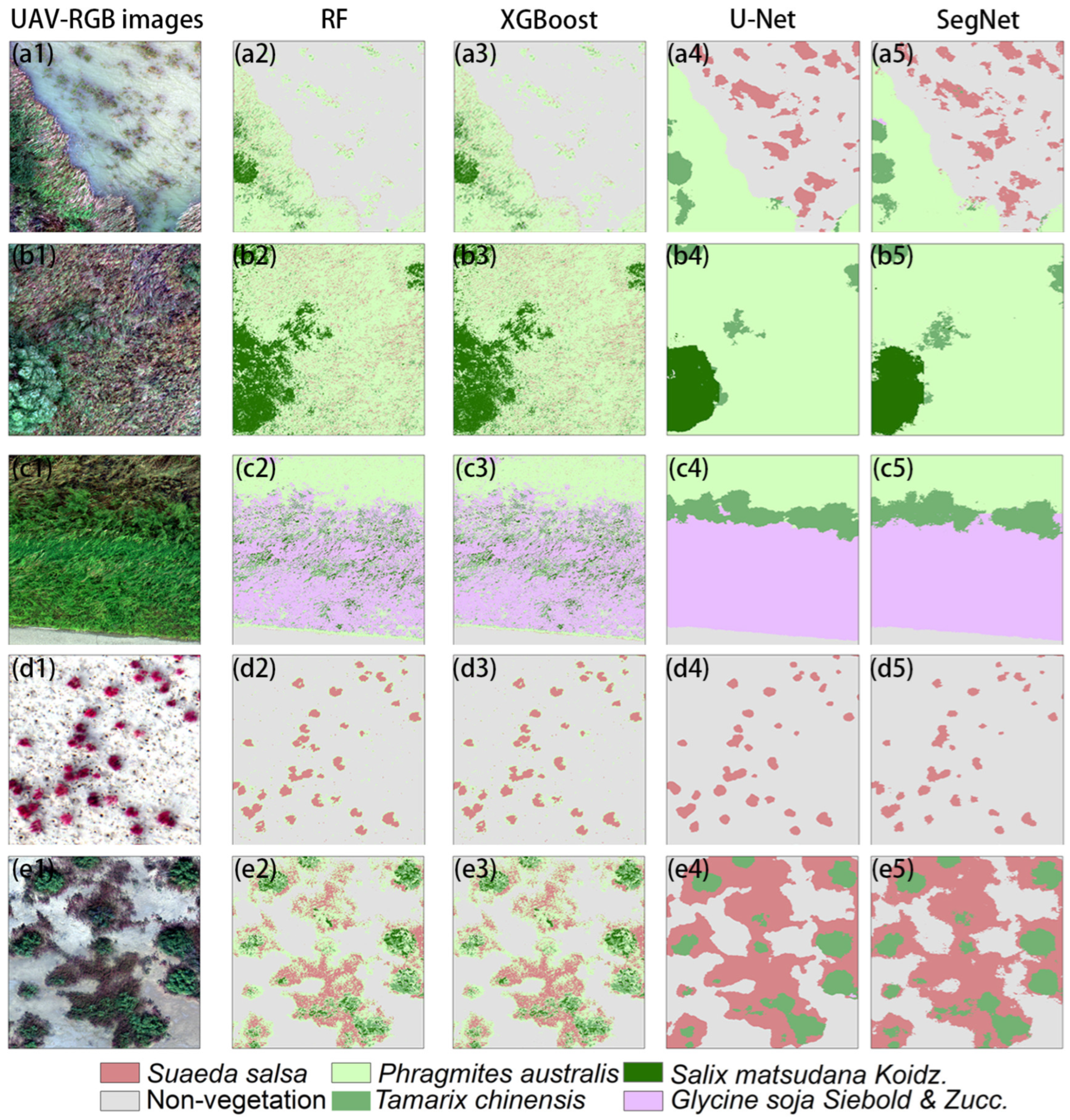
3.4. Comparison of Classification Accuracy Between Machine Learning and Deep Learning Models

A comparative analysis of U-Net, SegNet, XGBoost, and RF models across all species revealed that deep learning models outperformed machine learning models in salt marsh vegetation classification (Figure 6). U-Net demonstrated the highest performance across all metrics, with an OA of 94.05%, a Kappa of 0.9229, and an F1 Score of 0.9138. SegNet closely followed, achieving an OA of 93.26% and slightly lower Kappa and F1 scores. Regarding the machine learning models, RF performed a little better than XGBoost, with an OA of 83.74% compared to 83.34%.
Further investigation revealed that at the species level, the performance of deep learning models (U-Net and SegNet) also outperformed that of machine learning models (RF and XGBoost) in all species identification except for non-vegetation classes. U-Net recorded superior recall rates for Tamarix chinensis (80.12%) and Phragmites australis (94.09%), while SegNet showed higher recall rates for Suaeda salsa (93.3%) and Salix matsudana Koidz. (88.83%). U-Net also demonstrated excellent PA performance in identifying Suaeda salsa (92.38%) and Tamarix chinensis (82.76%), while SegNet gave higher PA in the separation of Phragmites australis (96.57%) and Salix matsudana Koidz. (94.44%). Both deep learning models showed consistent accuracy in identifying Glycine soja Siebold & Zucc.
Confusion matrix analysis further highlighted the advantages of deep learning models in reducing inter-class misclassification. With higher diagonal values in their confusion matrices, SegNet and U-Net demonstrated a superb ability to distinguish morphologically similar plant species (U-Net: 0.80–0.97; SegNet: 0.74–0.98) (Figure 7e,f). In contrast, RF and XGBoost showed notable confusion between Tamarix chinensis and Salix matsudana Koidz. Additionally, U-Net and SegNet exhibited an improved discrimination of Suaeda salsa, with diagonal values of 0.92 and 0.93, respectively, compared to 0.78 for both RF and XGBoost (Figure 7c and Figure 7d).
Traditional machine learning methods had obvious salt and pepper noise and misclassification phenomena. For example, Suaeda salsa patches in the Figure 8(d1) region were misclassified as Phragmites australis in RF (Figure 8(d2)) and XGBoost (Figure 8(d3)), while Tamarix chinensis in the b1 region was incorrectly labeled as Salix matsudana Koidz. in both RF (Figure 8(b2)) and XGBoost (Figure 8(b3)). These errors highlighted the limitations of traditional methods in distinguishing vegetation types with similar spectral features. In contrast, U-Net and SegNet deep learning models demonstrated superior performance, effectively reducing salt-and-pepper noise and enhancing spatial continuity in Suaeda salsa classifications (Figure 8(d4,d5)). However, the U-Net model produced overly distinct and abrupt boundaries between vegetation types (Figure 8(e4)), lacking the natural transitions found in real vegetation distributions. In contrast, the SegNet model excelled in boundary handling (Figure 8(e5)), better capturing the natural transitions between vegetation types.

4. Discussion

This study highlighted the significant ability of red and blue spectral bands to distinguish specific species [53,54], such as Tamarix chinensis and Phragmites australis, contrasting with previous studies that emphasized the dominant role of NIR bands [55,56]. Among vegetation indices, the superior performance of NDVI, OSAVI, and GCC can be attributed to the unique phenological and morphological characteristics of the vegetation during sampling. Chlorophyll-sensitive indices (NDVI and OSAVI) demonstrated effectiveness in distinguishing mature Suaeda salsa (exhibiting high red-light reflectance) from chlorophyll-rich species such as Glycine soja Siebold & Zucc. and Salix matsudana Koidz. These findings aligned with prior research showing that NDVI values for Suaeda salsa communities in August and September are significantly lower than those of other salt marsh vegetation [57]. Furthermore, Phragmites australis, with partially senescent leaves, exhibited moderate NDVI and OSAVI values, forming unique spectral features critical for its identification [58]. This finding was consistent with previous study documented seasonal variations in the spectral indices of coastal wetland vegetation [29]. Notably, canopy structure differences among vegetation types further enhanced the discriminative power of these indices. For example, variations in canopy structure, ranging from the short but dense Tamarix chinensis to the tall and lush Salix matsudana Koidz., were effectively reflected in NDVI and OSAVI. Additionally, GCC excelled in distinguishing Glycine soja Siebold & Zucc. and Salix matsudana Koidz. from the reddish Suaeda salsa and yellowing Phragmites australis. This aligned with earlier studies demonstrating that GCC effectively captures vegetation responses to environmental conditions and phenological changes [59]. These findings emphasize the importance of selecting appropriate spectral bands and vegetation indices for accurately classifying salt marsh vegetation in terms of ecosystem management and restoration efforts.
Deep learning models, particularly U-Net and SegNet, relatively outperformed traditional machine learning algorithms such as RF and XGBoost in classification accuracy, spatial detail, and overall robustness. The achieved accuracies (U-Net: 94.05%, SegNet: 93.26%) exceeded previously reported results, such as the 93% accuracy of U-Net in mapping Spartina alterniflora using Zhuhai-1 hyperspectral satellite imagery (32 spectral bands covering 400–1000 nm wavelengths with 10 m spatial resolution and 2.5 nm spectral resolution) [60] and the 87.34% accuracy of SegNet in mapping karst wetland vegetation [61]. This improvement demonstrated the potential of combining high-resolution UAV imagery with advanced deep-learning architectures to address the challenges of complex wetland environment identification. This superiority stemmed from their hierarchical feature-learning capabilities, which enabled the automatic extraction of complex spatial-spectral patterns from raw imagery, surpassing the limitations of predefined features in traditional methods [62]. While both machine learning and deep learning approaches were evaluated on datasets of the same scale in our study, their performance differences can be attributed to several key factors. Traditional machine learning models (RF and XGBoost) rely on predefined vegetation indices as input features, which, despite being carefully selected based on domain knowledge, may not capture all the complex spatial and contextual patterns present in salt marsh vegetation. These models excel in computational efficiency and interpretability, making them valuable for applications with limited computational resources. However, their reliance on manually engineered features restricts their ability to model complex vegetation distributions. In contrast, deep learning models (U-Net and SegNet) automatically learn hierarchical feature representations directly from raw spectral data through convolutional layers. This automated feature extraction capability enables them to capture subtle spatial relationships and morphological characteristics crucial for distinguishing morphologically similar species. The encoder-decoder architectures of U-Net and SegNet leverage multi-scale contextual information through skip connections and pooling indices, respectively, resulting in more robust feature representations [63]. This architectural advantage was evident in distinguishing morphologically similar species, such as Tamarix chinensis and Salix matsudana Koidz., whereas traditional methods exhibited significant confusion. While RF and XGBoost demonstrated lower classification accuracies, they provided interpretability advantages through feature importance rankings, complementing the ‘black-box’ nature of deep learning approaches. In addition, U-Net excelled at integrating low-level spatial information through skip connections, achieving higher accuracy for structurally complex species (Tamarix chinensis: 80.12%, Phragmites australis: 94.09%) [64]. However, this sometimes resulted in abrupt boundaries between vegetation types (Figure 8(e4)). In contrast, SegNet’s pooling index-based upsampling produced smoother transition zones (Figure 8(e5)), better reflecting the gradual vegetation transitions. This trade-off between detail preservation and boundary naturalization is a critical consideration when selecting models for specific applications.
Several limitations should be addressed in future research. First, this analysis primarily relied on spectral features and vegetation indices without incorporating texture and morphological features, which previous studies have shown to significantly improve vegetation classification [65,66]. Second, the portability of our UAV-based approach is limited, as its high spatial resolution may not be directly applicable to medium- or high-resolution satellite imagery for large-scale monitoring. This limitation stems from two primary factors: (1) the significant resolution disparity between UAV imagery (centimeter-level) and satellite imagery (meter-level), which prevents satellites from capturing the fine-scale vegetation patterns and subtle boundaries detectable with UAVs, and (2) the spectral characteristics of UAV and satellite sensors differ, even when using the same vegetation indices. While these indices are standard and can be applied across platforms, the way they reflect vegetation features varies significantly depending on whether the data come from high-resolution UAV imagery or coarser satellite imagery. The technical challenges identified in UAV platforms, including insufficient flight stability, limited endurance, vulnerability to external interference, and inadequate payload capacity, further contribute to the portability limitations of UAVs. Future studies should focus on enhancing UAV technology, particularly by improving flight stability and endurance through advanced control systems and battery technologies, reducing vulnerability to external interference through robust GPS and communication systems, and increasing payload capacity through the miniaturization of remote sensing instruments. Additionally, this study was also limited to a small area of the Yellow River Delta and a single sampling period (September), potentially missing seasonal spectral variations that could improve classification accuracy. Future studies should focus on multi-temporal analyses to capture phenological changes and assess the robustness of classification methods across varying seasons and environmental conditions. Encompassing diverse ecological settings and vegetation communities will improve the generalizability of the findings, offering a more comprehensive understanding of salt marsh vegetation patterns.

5. Conclusions

This study utilized high-resolution UAV imagery to investigate the characteristic differences among salt marsh vegetation types and compare the performance of machine learning and deep learning methods in vegetation classification. The spectral analysis underscored the critical role of vegetation indices, such as NDVI, GNDVI, and OSAVI, in species differentiation, with particular attention to the ability of specific spectral bands, including red and blue, to improve classification. This insight offers a novel perspective compared to previous studies that predominantly focused on the role of NIR bands. Deep learning models, especially U-Net, outperformed traditional machine learning models in overall classification accuracy, achieving a maximum accuracy of 94.05%. These models exhibited significant advantages in spatial recognition, delivering more cohesive and homogeneous classification results, whereas traditional machine learning models struggled with complex spatial relationships. By integrating high-resolution UAV multispectral data with advanced deep learning techniques, this study demonstrates the potential of combining these technologies to enhance coastal ecological monitoring. The approach represents a significant improvement over traditional machine learning methods, offering a more accurate and scalable solution for vegetation classification. However, limitations such as restricted spatiotemporal coverage and the exclusion of environmental factors highlight the need for future research to address these gaps, particularly through multi-temporal analyses and the integration of external environmental variables.

Author Contributions

Conceptualization, S.R.; Methodology, X.B.; Formal analysis, X.B.; Data curation, X.B.; Data collection, C.Y., L.F., J.C., X.W., N.G. and P.Z.; Writing—original draft preparation, X.B.; Writing—reviewing and editing, S.R., G.W., Q.W., C.Y., L.F., J.C., X.W., N.G. and P.Z. All authors have read and agreed to the published version of the manuscript.

Funding

This study is supported by the National Key R&D Program of China (No. 2022YFC3204400).

Data Availability Statement

The research data will be shared when accepted.

Conflicts of Interest

The authors declare no conflicts of interest.

References

  1. Barbier, E.B.; Hacker, S.D.; Kennedy, C.; Koch, E.W.; Stier, A.C.; Silliman, B.R. The value of estuarine and coastal ecosystem services. Ecol. Monogr. 2011, 81, 169–193. [Google Scholar] [CrossRef]
  2. Fagherazzi, S.; Kirwan, M.L.; Mudd, S.M.; Guntenspergen, G.R.; Temmerman, S.; D’Alpaos, A.; Van De Koppel, J.; Rybczyk, J.M.; Reyes, E.; Craft, C. Numerical models of salt marsh evolution: Ecological, geomorphic, and climatic factors. Rev. Geophys. 2012, 50, RG1002. [Google Scholar]
  3. Lou, Y.; Dai, Z.; Long, C.; Dong, H.; Wei, W.; Ge, Z. Image-based machine learning for monitoring the dynamics of the largest salt marsh in the Yangtze River Delta. J. Hydrol. 2022, 608, 127681. [Google Scholar] [CrossRef]
  4. Balke, T.; Stock, M.; Jensen, K.; Bouma, T.J.; Kleyer, M. A global analysis of the seaward salt marsh extent: The importance of tidal range. Water Resour. Res. 2016, 52, 3775–3786. [Google Scholar] [CrossRef]
  5. Stückemann, K.-J.; Waske, B. Mapping Lower Saxony’s salt marshes using temporal metrics of multi-sensor satellite data. Int. J. Appl. Earth Obs. Geoinf. 2022, 115, 103123. [Google Scholar] [CrossRef]
  6. Temmerman, S.; Meire, P.; Bouma, T.J.; Herman, P.M.; Ysebaert, T.; De Vriend, H.J. Ecosystem-based coastal defence in the face of global change. Nature 2013, 504, 79–83. [Google Scholar]
  7. Sun, H.; Jiang, J.; Cui, L.; Feng, W.; Wang, Y.; Zhang, J. Soil organic carbon stabilization mechanisms in a subtropical mangrove and salt marsh ecosystems. Sci. Total Environ. 2019, 673, 502–510. [Google Scholar] [CrossRef]
  8. Chen, X.; Zhang, M.; Zhang, W. Landscape pattern changes and its drivers inferred from salt marsh plant variations in the coastal wetlands of the Liao River Estuary, China. Ecol. Indic. 2022, 145, 109719. [Google Scholar] [CrossRef]
  9. Huang, Y.; Zheng, G.; Li, X.; Xiao, J.; Xu, Z.; Tian, P. Habitat quality evaluation and pattern simulation of coastal salt marsh wetlands. Sci. Total Environ. 2024, 945, 174003. [Google Scholar]
  10. Mason, V.G.; Burden, A.; Epstein, G.; Jupe, L.L.; Wood, K.A.; Skov, M.W. Blue carbon benefits from global saltmarsh restoration. Glob. Change Biol. 2023, 29, 6517–6545. [Google Scholar]
  11. Leahy, M.G.; Jollineau, M.Y.; Howarth, P.J.; Gillespie, A.R. The use of Landsat data for investigating the long-term trends in wetland change at Long Point, Ontario. Can. J. Remote Sens. 2005, 31, 240–254. [Google Scholar] [CrossRef]
  12. Slagter, B.; Tsendbazar, N.-E.; Vollrath, A.; Reiche, J. Mapping wetland characteristics using temporally dense Sentinel-1 and Sentinel-2 data: A case study in the St. Lucia wetlands, South Africa. Int. J. Appl. Earth Obs. Geoinf. 2020, 86, 102009. [Google Scholar] [CrossRef]
  13. Pan, Y.; Xu, X.; Long, J.; Lin, H. Change detection of wetland restoration in China’s Sanjiang National Nature Reserve using STANet method based on GF-1 and GF-6 images. Ecol. Indic. 2022, 145, 109612. [Google Scholar] [CrossRef]
  14. Li, H.; Liu, Q.; Huang, C.; Zhang, X.; Wang, S.; Wu, W.; Shi, L. Variation in Vegetation Composition and Structure across Mudflat Areas in the Yellow River Delta, China. Remote Sens. 2024, 16, 3495. [Google Scholar] [CrossRef]
  15. Chen, J.; Chen, Z.; Huang, R.; You, H.; Han, X.; Yue, T.; Zhou, G. The Effects of Spatial Resolution and Resampling on the Classification Accuracy of Wetland Vegetation Species and Ground Objects: A Study Based on High Spatial Resolution UAV Images. Drones 2023, 7, 61. [Google Scholar] [CrossRef]
  16. Villoslada, M.; Bergamo, T.F.; Ward, R.; Burnside, N.; Joyce, C.; Bunce, R.; Sepp, K. Fine scale plant community assessment in coastal meadows using UAV based multispectral data. Ecol. Indic. 2020, 111, 105979. [Google Scholar] [CrossRef]
  17. Zheng, J.-Y.; Hao, Y.-Y.; Wang, Y.-C.; Zhou, S.-Q.; Wu, W.-B.; Yuan, Q.; Gao, Y.; Guo, H.-Q.; Cai, X.-X.; Zhao, B. Coastal wetland vegetation classification using pixel-based, object-based and deep learning methods based on RGB-UAV. Land 2022, 11, 2039. [Google Scholar] [CrossRef]
  18. Zhou, Z.; Yang, Y.; Chen, B. Estimating Spartina alterniflora fractional vegetation cover and aboveground biomass in a coastal wetland using SPOT6 satellite and UAV data. Aquat. Bot. 2018, 144, 38–45. [Google Scholar] [CrossRef]
  19. Detka, J.; Coyle, H.; Gomez, M.; Gilbert, G.S. A drone-powered deep learning methodology for high precision remote sensing in California’s coastal shrubs. Drones 2023, 7, 421. [Google Scholar] [CrossRef]
  20. Simpson, G.; Nichol, C.J.; Wade, T.; Helfter, C.; Hamilton, A.; Gibson-Poole, S. Species-Level Classification of Peatland Vegetation Using Ultra-High-Resolution UAV Imagery. Drones 2024, 8, 97. [Google Scholar] [CrossRef]
  21. Patil, M.B.; Desai, C.G.; Umrikar, B.N. Image classification tool for land use/land cover analysis: A comparative study of maximum likelihood and minimum distance method. Int. J. Geol. Earth Environ. Sci. 2012, 2, 189–196. [Google Scholar]
  22. Sanchez-Hernandez, C.; Boyd, D.S.; Foody, G.M. Mapping specific habitats from remotely sensed imagery: Support vector machine and support vector data description based classification of coastal saltmarsh habitats. Ecol. Inform. 2007, 2, 83–88. [Google Scholar] [CrossRef]
  23. Rodriguez-Galiano, V.F.; Chica-Olmo, M.; Abarca-Hernandez, F.; Atkinson, P.M.; Jeganathan, C. Random Forest classification of Mediterranean land cover using multi-seasonal imagery and multi-seasonal texture. Remote Sens. Environ. 2012, 121, 93–107. [Google Scholar] [CrossRef]
  24. Shi, F.; Gao, X.; Li, R.; Zhang, H. Ensemble Learning for the Land Cover Classification of Loess Hills in the Eastern Qinghai–Tibet Plateau Using GF-7 Multitemporal Imagery. Remote Sens. 2024, 16, 2556. [Google Scholar] [CrossRef]
  25. Van Beijma, S.; Comber, A.; Lamb, A. Random forest classification of salt marsh vegetation habitats using quad-polarimetric airborne SAR, elevation and optical RS data. Remote Sens. Environ. 2014, 149, 118–129. [Google Scholar] [CrossRef]
  26. Li, H.; Wang, C.; Cui, Y.; Hodgson, M. Mapping salt marsh along coastal South Carolina using U-Net. ISPRS J. Photogramm. Remote Sens. 2021, 179, 121–132. [Google Scholar] [CrossRef]
  27. Dang, K.B.; Nguyen, M.H.; Nguyen, D.A.; Phan, T.T.H.; Giang, T.L.; Pham, H.H.; Nguyen, T.N.; Tran, T.T.V.; Bui, D.T. Coastal wetland classification with deep u-net convolutional networks and sentinel-2 imagery: A case study at the tien yen estuary of vietnam. Remote Sens. 2020, 12, 3270. [Google Scholar] [CrossRef]
  28. Xing, H.; Niu, J.; Feng, Y.; Hou, D.; Wang, Y.; Wang, Z. A coastal wetlands mapping approach of Yellow River Delta with a hierarchical classification and optimal feature selection framework. Catena 2023, 223, 106897. [Google Scholar] [CrossRef]
  29. Zhang, C.; Gong, Z.; Qiu, H.; Zhang, Y.; Zhou, D. Mapping typical salt-marsh species in the Yellow River Delta wetland supported by temporal-spatial-spectral multidimensional features. Sci. Total Environ. 2021, 783, 147061. [Google Scholar] [CrossRef]
  30. Chen, C.; Ma, Y.; Yu, D.; Hu, Y.; Ren, L. Tracking annual dynamics of carbon storage of salt marsh plants in the Yellow River Delta national nature reserve of china based on sentinel-2 imagery during 2017–2022. Int. J. Appl. Earth Obs. Geoinf. 2024, 130, 103880. [Google Scholar] [CrossRef]
  31. Wang, Z.; Ke, Y.; Lu, D.; Zhuo, Z.; Zhou, Q.; Han, Y.; Sun, P.; Gong, Z.; Zhou, D. Estimating fractional cover of saltmarsh vegetation species in coastal wetlands in the Yellow River Delta, China using ensemble learning model. Front. Mar. Sci. 2022, 9, 1077907. [Google Scholar] [CrossRef]
  32. Li, J.; Hussain, T.; Feng, X.; Guo, K.; Chen, H.; Yang, C.; Liu, X. Comparative study on the resistance of Suaeda glauca and Suaeda salsa to drought, salt, and alkali stresses. Ecol. Eng. 2019, 140, 105593. [Google Scholar]
  33. Kiviat, E. Ecosystem services of Phragmites in North America with emphasis on habitat functions. AoB Plants 2013, 5, plt008. [Google Scholar]
  34. Yang, H.; Xia, J.; Cui, Q.; Liu, J.; Wei, S.; Feng, L.; Dong, K. Effects of different Tamarix chinensis-grass patterns on the soil quality of coastal saline soil in the Yellow River Delta, China. Sci. Total Environ. 2021, 772, 145501. [Google Scholar] [PubMed]
  35. Jiang, Z.; Huete, A.R.; Chen, J.; Chen, Y.; Li, J.; Yan, G.; Zhang, X. Analysis of NDVI and scaled difference vegetation index retrievals of vegetation fraction. Remote Sens. Environ. 2006, 101, 366–378. [Google Scholar]
  36. García Cárdenas, D.A.; Ramón Valencia, J.A.; Alzate Velásquez, D.F.; Palacios Gonzalez, J.R. Dynamics of the indices NDVI and GNDVI in a rice growing in its reproduction phase from multi-spectral aerial images taken by drones. In Proceedings of the International Conference of ICT for Adapting Agriculture to Climate Change, Cali, Colombia, 21–23 November 2018; pp. 106–119. [Google Scholar]
  37. Davidson, C.; Jaganathan, V.; Sivakumar, A.N.; Czarnecki, J.M.P.; Chowdhary, G. NDVI/NDRE prediction from standard RGB aerial imagery using deep learning. Comput. Electron. Agric. 2022, 203, 107396. [Google Scholar]
  38. Hollberg, J.L.; Schellberg, J. Distinguishing intensity levels of grassland fertilization using vegetation indices. Remote Sens. 2017, 9, 81. [Google Scholar] [CrossRef]
  39. Steven, M.D. The sensitivity of the OSAVI vegetation index to observational parameters. Remote Sens. Environ. 1998, 63, 49–60. [Google Scholar] [CrossRef]
  40. Burke, M.W.; Rundquist, B.C. Scaling PhenoCam GCC, NDVI, and EVI2 with harmonized Landsat-Sentinel using Gaussian processes. Agric. For. Meteorol. 2021, 300, 108316. [Google Scholar]
  41. Zeng, J.; Sun, Y.; Cao, P.; Wang, H. A phenology-based vegetation index classification (PVC) algorithm for coastal salt marshes using Landsat 8 images. Int. J. Appl. Earth Obs. Geoinf. 2022, 110, 102776. [Google Scholar]
  42. Canovas-Garcia, F.; Alonso-Sarria, F. Optimal combination of classification algorithms and feature ranking methods for object-based classification of submeter resolution Z/I-imaging DMC imagery. Remote Sens. 2015, 7, 4651–4677. [Google Scholar] [CrossRef]
  43. Shao, Y.; Lunetta, R.S.; Wheeler, B.; Iiames, J.S.; Campbell, J.B. An evaluation of time-series smoothing algorithms for land-cover classifications using MODIS-NDVI multi-temporal data. Remote Sens. Environ. 2016, 174, 258–265. [Google Scholar] [CrossRef]
  44. Phan, T.N.; Kuch, V.; Lehnert, L.W. Land cover classification using Google Earth Engine and random forest classifier—The role of image composition. Remote Sens. 2020, 12, 2411. [Google Scholar] [CrossRef]
  45. Speiser, J.L.; Miller, M.E.; Tooze, J.; Ip, E. A comparison of random forest variable selection methods for classification prediction modeling. Expert Syst. Appl. 2019, 134, 93–101. [Google Scholar]
  46. Chen, T.; Guestrin, C. Xgboost: A scalable tree boosting system. In Proceedings of the 22nd ACM SIGKDD International Conference on Knowledge Discovery and Data Mining, San Francisco, CA, USA, 13–17 August 2016; pp. 785–794. [Google Scholar]
  47. Ronneberger, O.; Fischer, P.; Brox, T. U-net: Convolutional networks for biomedical image segmentation. In Proceedings of the Medical Image Computing and Computer-Assisted Intervention–MICCAI 2015: 18th International Conference, Munich, Germany, 5–9 October 2015; Proceedings, Part III. pp. 234–241. [Google Scholar]
  48. Bragagnolo, L.; da Silva, R.V.; Grzybowski, J.M.V. Amazon forest cover change mapping based on semantic segmentation by U-Nets. Ecol. Inform. 2021, 62, 101279. [Google Scholar]
  49. Wang, J.; Hadjikakou, M.; Hewitt, R.J.; Bryan, B.A. Simulating large-scale urban land-use patterns and dynamics using the U-Net deep learning architecture. Comput. Environ. Urban Syst. 2022, 97, 101855. [Google Scholar] [CrossRef]
  50. Fu, B.; Liu, M.; He, H.; Lan, F.; He, X.; Liu, L.; Huang, L.; Fan, D.; Zhao, M.; Jia, Z. Comparison of optimized object-based RF-DT algorithm and SegNet algorithm for classifying Karst wetland vegetation communities using ultra-high spatial resolution UAV data. Int. J. Appl. Earth Obs. Geoinf. 2021, 104, 102553. [Google Scholar] [CrossRef]
  51. Deng, T.; Fu, B.; Liu, M.; He, H.; Fan, D.; Li, L.; Huang, L.; Gao, E. Comparison of multi-class and fusion of multiple single-class SegNet model for mapping karst wetland vegetation using UAV images. Sci. Rep. 2022, 12, 13270. [Google Scholar]
  52. Diederik, P.K. Adam: A method for stochastic optimization. arXiv 2014, arXiv:1412.6980. [Google Scholar]
  53. Chen, C.; Yuan, X.; Gan, S.; Luo, W.; Bi, R.; Li, R.; Gao, S. A new vegetation index based on UAV for extracting plateau vegetation information. Int. J. Appl. Earth Obs. Geoinf. 2024, 128, 103668. [Google Scholar]
  54. Schmidt, K.; Skidmore, A. Spectral discrimination of vegetation types in a coastal wetland. Remote Sens. Environ. 2003, 85, 92–108. [Google Scholar] [CrossRef]
  55. Liu, M.; Zhan, Y.; Li, J.; Kang, Y.; Sun, X.; Gu, X.; Wei, X.; Wang, C.; Li, L.; Gao, H. Validation of Red-Edge Vegetation Indices in Vegetation Classification in Tropical Monsoon Region—A Case Study in Wenchang, Hainan, China. Remote Sens. 2024, 16, 1865. [Google Scholar] [CrossRef]
  56. Zahir, S.A.D.M.; Omar, A.F.; Jamlos, M.F.; Azmi, M.A.M.; Muncan, J. A review of visible and near-infrared (Vis-NIR) spectroscopy application in plant stress detection. Sens. Actuators A Phys. 2022, 338, 113468. [Google Scholar] [CrossRef]
  57. Sun, C.; Liu, Y.; Zhao, S.; Zhou, M.; Yang, Y.; Li, F. Classification mapping and species identification of salt marshes based on a short-time interval NDVI time-series from HJ-1 optical imagery. Int. J. Appl. Earth Obs. Geoinf. 2016, 45, 27–41. [Google Scholar] [CrossRef]
  58. Wu, N.; Shi, R.; Zhuo, W.; Zhang, C.; Zhou, B.; Xia, Z.; Tao, Z.; Gao, W.; Tian, B. A classification of tidal flat wetland vegetation combining phenological features with Google Earth Engine. Remote Sens. 2021, 13, 443. [Google Scholar] [CrossRef]
  59. Woebbecke, D.M.; Meyer, G.E.; Von Bargen, K.; Mortensen, D.A. Color indices for weed identification under various soil, residue, and lighting conditions. Trans. ASAE 1995, 38, 259–269. [Google Scholar] [CrossRef]
  60. Li, H.; Cui, G.; Liu, H.; Wang, Q.; Zhao, S.; Huang, X.; Zhang, R.; Jia, M.; Mao, D.; Yu, H. Dynamic Analysis of Spartina alterniflora in Yellow River Delta Based on U-Net Model and Zhuhai-1 Satellite. Remote Sens. 2025, 17, 226. [Google Scholar] [CrossRef]
  61. Fu, B.; Liu, M.; He, H.; Fan, D.; Liu, L.; Huang, L.; Gao, E. Comparison of Multi-class and Fusion of single-class SegNet model for Classifying Karst Wetland Vegetation using UAV Images. Preprints 2021. [Google Scholar] [CrossRef]
  62. Bhatnagar, S.; Gill, L.; Ghosh, B. Drone image segmentation using machine and deep learning for mapping raised bog vegetation communities. Remote Sens. 2020, 12, 2602. [Google Scholar] [CrossRef]
  63. Fan, X.; Yan, C.; Fan, J.; Wang, N. Improved U-net remote sensing classification algorithm fusing attention and multiscale features. Remote Sens. 2022, 14, 3591. [Google Scholar] [CrossRef]
  64. Wang, H.; Gui, D.; Liu, Q.; Feng, X.; Qu, J.; Zhao, J.; Wang, G.; Wei, G. Vegetation coverage precisely extracting and driving factors analysis in drylands. Ecol. Inform. 2024, 79, 102409. [Google Scholar]
  65. Chiu, W.-Y.; Couloigner, I. Evaluation of incorporating texture into wetland mapping from multispectral images. EARSeL eProceedings 2004, 3, 363–371. [Google Scholar]
  66. Murray, H.; Lucieer, A.; Williams, R. Texture-based classification of sub-Antarctic vegetation communities on Heard Island. Int. J. Appl. Earth Obs. Geoinf. 2010, 12, 138–149. [Google Scholar]
Figure 1. Orthophoto displayed in RGB mode; (ac) show portions of the orthophoto captured at different representative sampling points in the Yellow River Delta; (c1c3) represent different sections of the orthophoto taken from the same region (c). The aerial image represents the multispectral orthophoto with a spatial resolution of 2 cm, captured on 14–15 September 2024, using a DJI Phantom 4 Multispectral drone.
Drones 09 00235 g001
Figure 2. Comparison of (a) spectral features and (b) vegetation indices among different vegetation types.
Drones 09 00235 g002
Figure 3. The Jeffries–Matusita (JM) distances between pairs of species.
Drones 09 00235 g003
Figure 4. Importance ranking of all spectral and index features.
Drones 09 00235 g004
Figure 5. Training process comparison of deep learning models. (a) Accuracy; (b) Loss.
Drones 09 00235 g005
Figure 6. Overall accuracy evaluation among machine learning and deep learning models.
Drones 09 00235 g006
Figure 7. Accuracy evaluation of machine learning and deep learning models at the species level; (a) recall rate and (b) PA for different vegetation categories; (cf) confusion matrices of RF, XGBoost, U-net, and SegNet model, respectively.
Drones 09 00235 g007
Figure 8. Spatial pattern comparison of vegetation classification using U-Net, SegNet, RF, and XGBoost model; (a1,b1,c1,d1,e1) show UAV-RGB images; (a2,b2,c2,d2,e2) are RF-based classification results; (a3,b3,c3,d3,e3) are XGBoost-based classification results; (a4,b4,c4,d4,e4) are U-Net-based classification results; and (a5,b5,c5,d5,e5) are SegNet-based classification results.
Drones 09 00235 g008
Table 1. Species description and UAV image example (RGB). Note: Species images were sourced from the Plant Photo Bank of China (PPBC, https://ppbc.iplant.cn/), accessed on 20 January 2025.
ClassClass DescriptionUAV Image Example (RGB)
Suaeda salsaPrimarily grows in mid-tide and low-tide zones, with varying vegetation coverage.
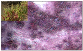
Drones 09 00235 i001
Tamarix chinensisLives in moist saline-alkali soils, with a growing season from April to November.
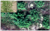
Drones 09 00235 i002
Phragmites australisDistributes along water shores, with a growing season from April to October.Drones 09 00235 i003
Glycinesoja Siebold & Zucc.Popular in low-lying, wetland areas with dense shrubs or Phragmites australis reed beds, with a growing season from March to October.Drones 09 00235 i004
Salix matsudana Koidz.Common in arid lands or wetlands, with a rapid growth period from June to July.
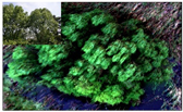
Drones 09 00235 i005
Table 2. Number and proportions of labeled pixels for the five salt marsh vegetation classes used for deep learning and machine learning.
ClassDeep LearningMachine Learning
Labeled PixelsPercentage (%)Labeled PixelsPercentage (%)
Suaeda salsa3,973,63114.7169,3986.87
Tamarix chinensis2,618,8549.69257,24025.48
Phragmites australis7,790,03228.84109,56910.85
Glycine soja Siebold & Zucc.6,606,23224.45103,26610.23
Salix matsudana Koidz.175,0380.65154,21715.28
Non-vegetation5,851,44321.66315,90831.29
Disclaimer/Publisher’s Note: The statements, opinions and data contained in all publications are solely those of the individual author(s) and contributor(s) and not of MDPI and/or the editor(s). MDPI and/or the editor(s) disclaim responsibility for any injury to people or property resulting from any ideas, methods, instructions or products referred to in the content.

