Author Contributions
Conceptualization, X.L. and L.G.; methodology, X.L., L.G. and Y.Z.; software, X.L. and Y.Z.; validation, K.L.; formal analysis, X.L.; investigation, X.L. and Y.Z.; resources, K.L.; writing—original draft preparation, X.L.; writing—review and editing, X.L., L.G. and K.L.; visualization, X.L.; supervision, L.G. and K.L.; project administration, L.G. and K.L.; funding acquisition, K.L. All authors have read and agreed to the published version of the manuscript.
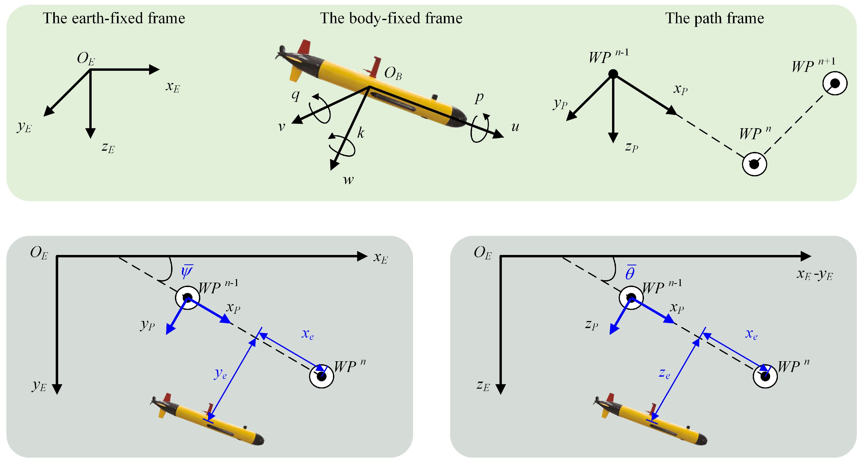
Figure 1.
Illustration of the path-following mission of AUV.
Figure 1.
Illustration of the path-following mission of AUV.
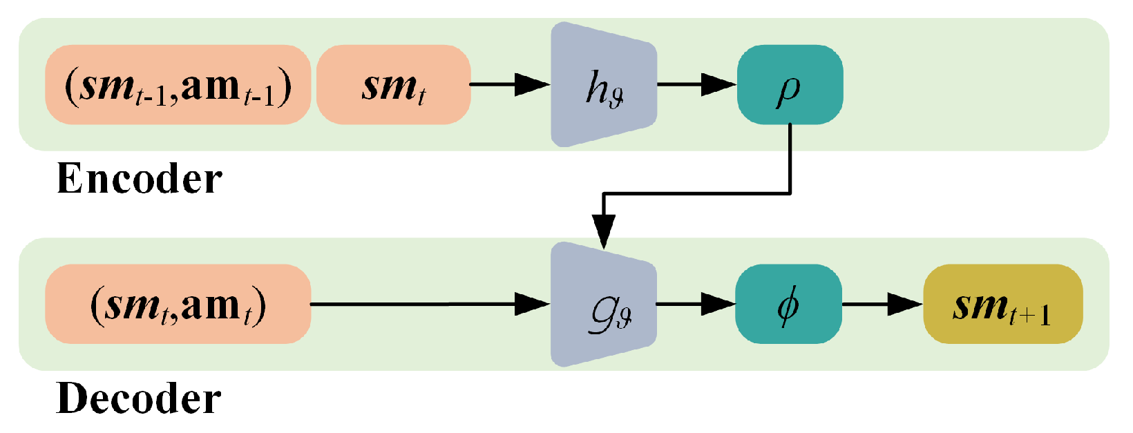
Figure 2.
Schematic representation of the CNP.
Figure 2.
Schematic representation of the CNP.
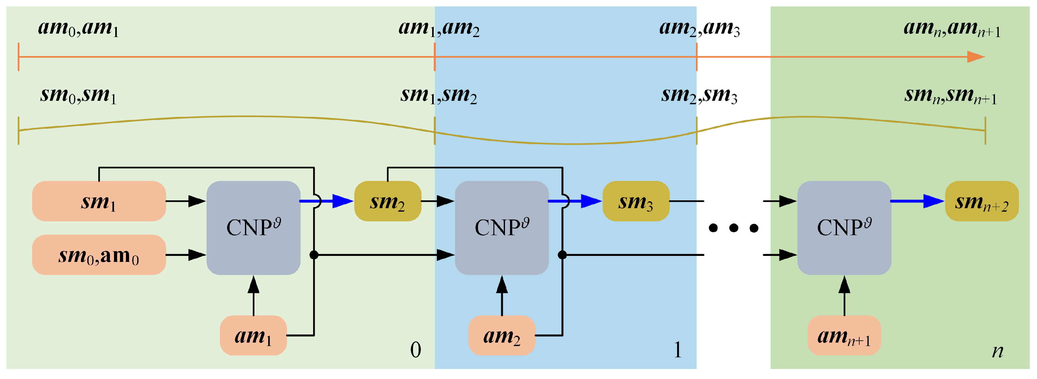
Figure 3.
Schematic representation of the N-step recurrent iterative training method.
Figure 3.
Schematic representation of the N-step recurrent iterative training method.
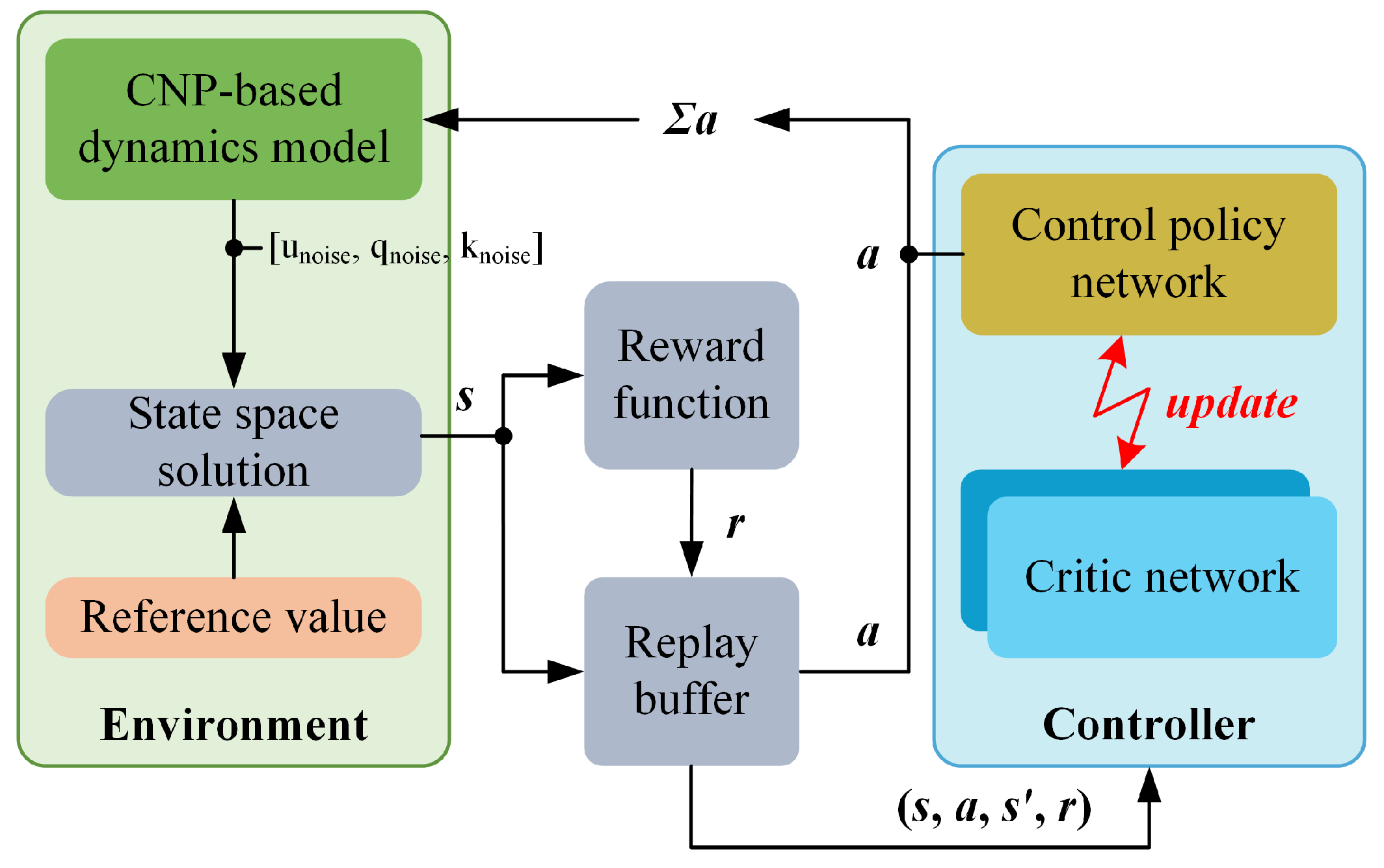
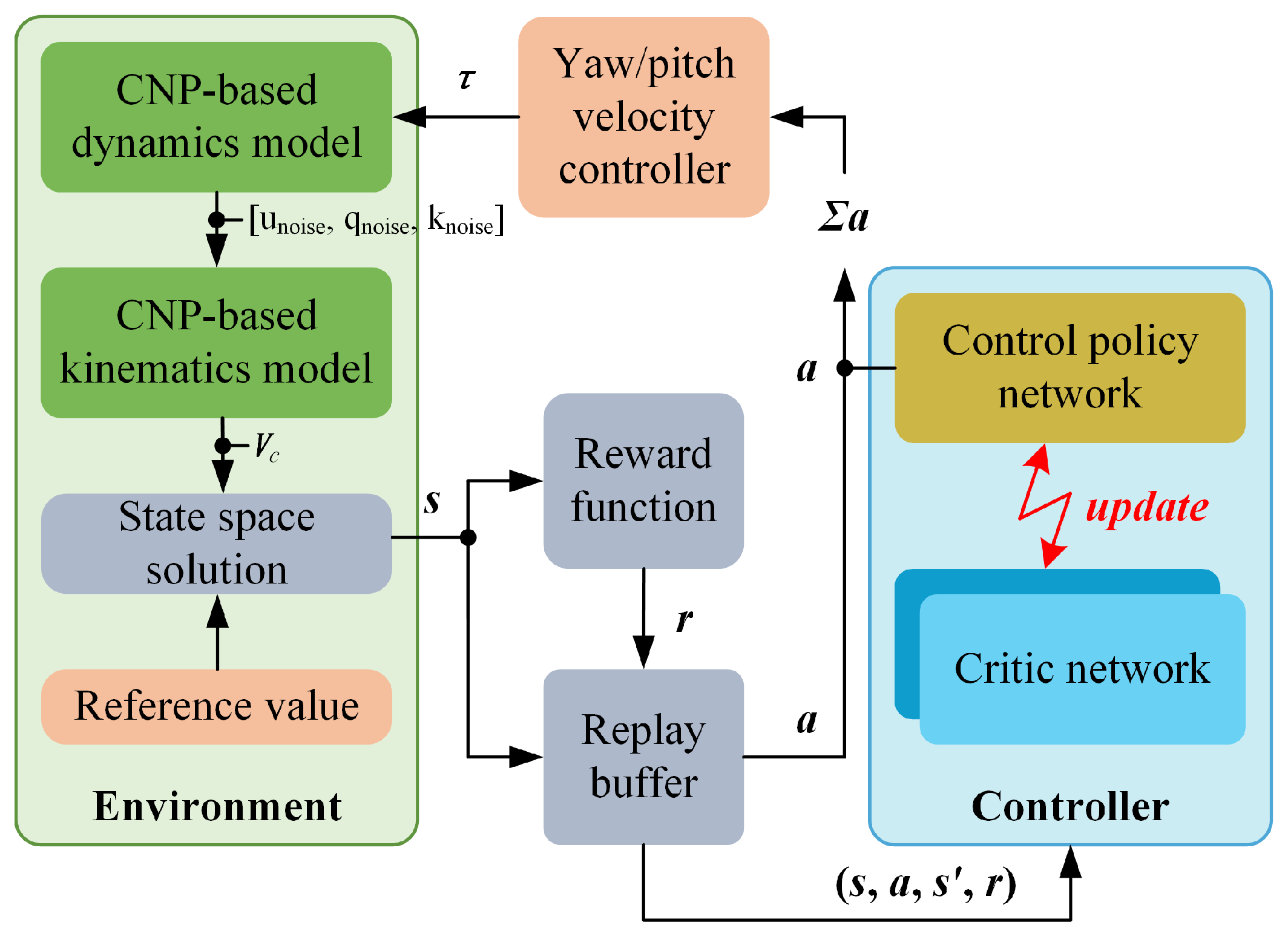
Figure 4.
Overall structure of the proposed control.
Figure 4.
Overall structure of the proposed control.
Figure 5.
Control policy learning schematic representation of the velocity controllers.
Figure 5.
Control policy learning schematic representation of the velocity controllers.
Figure 6.
Control policy learning schematic representation of the path-following controller.
Figure 6.
Control policy learning schematic representation of the path-following controller.
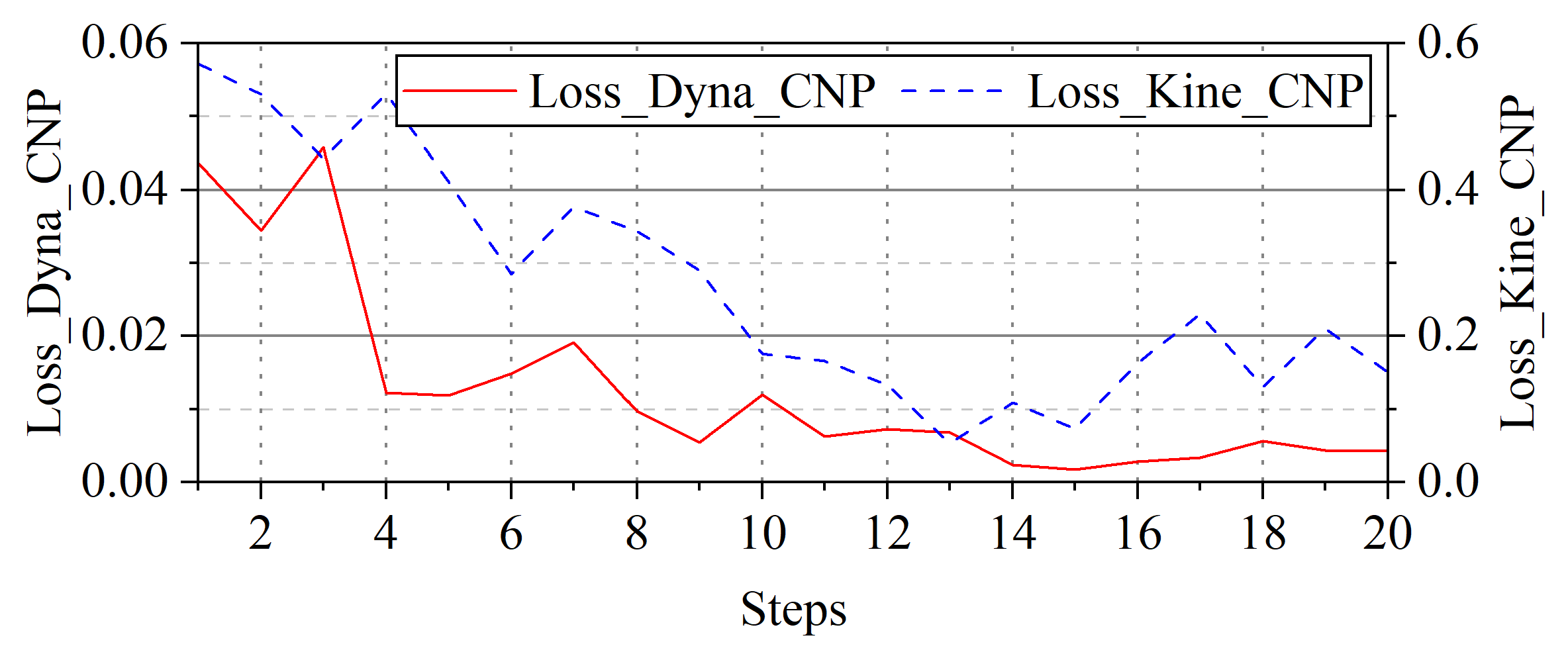
Figure 7.
Impact of the recurrent prediction steps during each iteration on convergence.
Figure 7.
Impact of the recurrent prediction steps during each iteration on convergence.
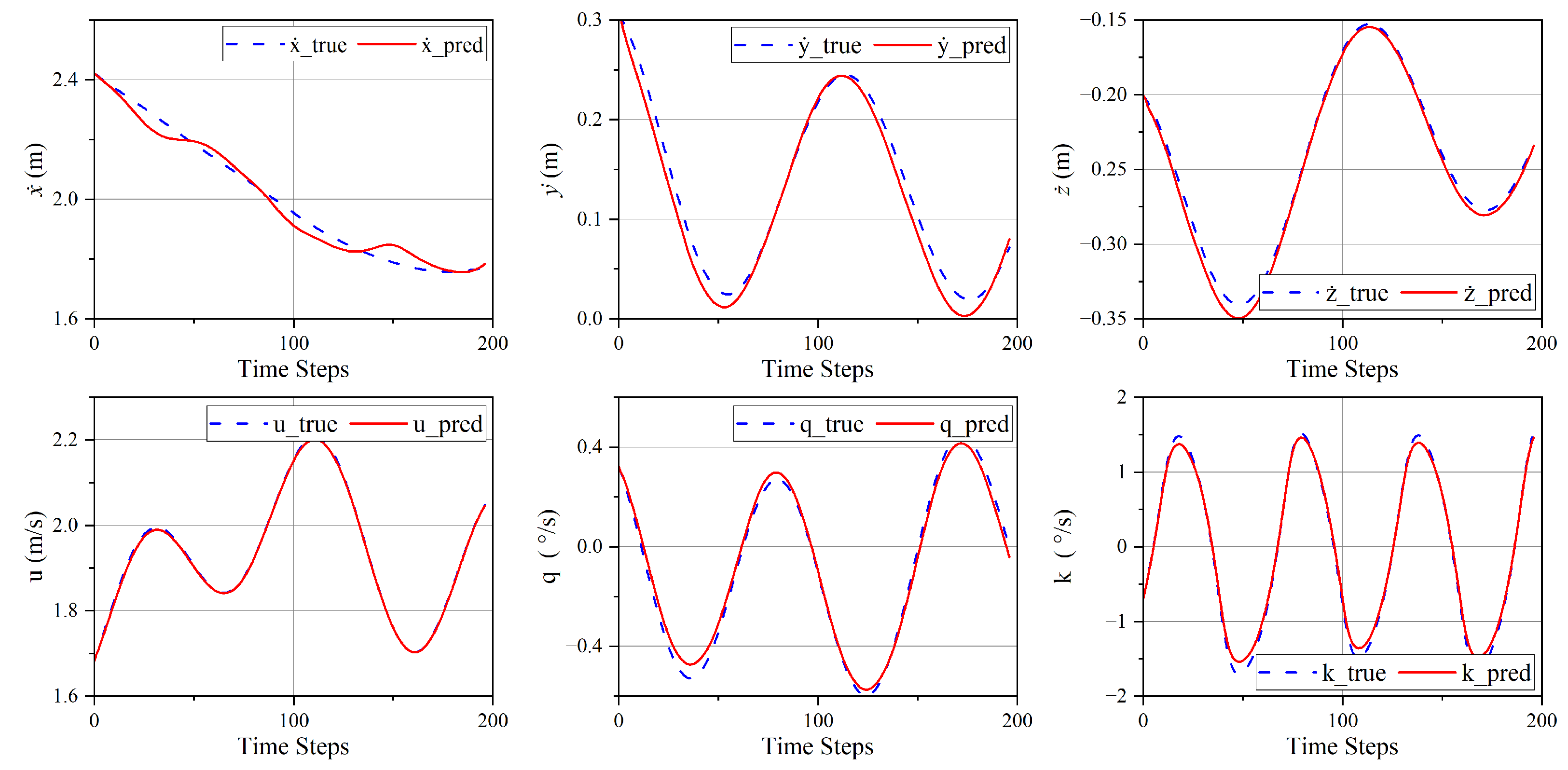
Figure 8.
Prediction results of AUV motion states by the CNP-based dynamics and kinematics models.
Figure 8.
Prediction results of AUV motion states by the CNP-based dynamics and kinematics models.
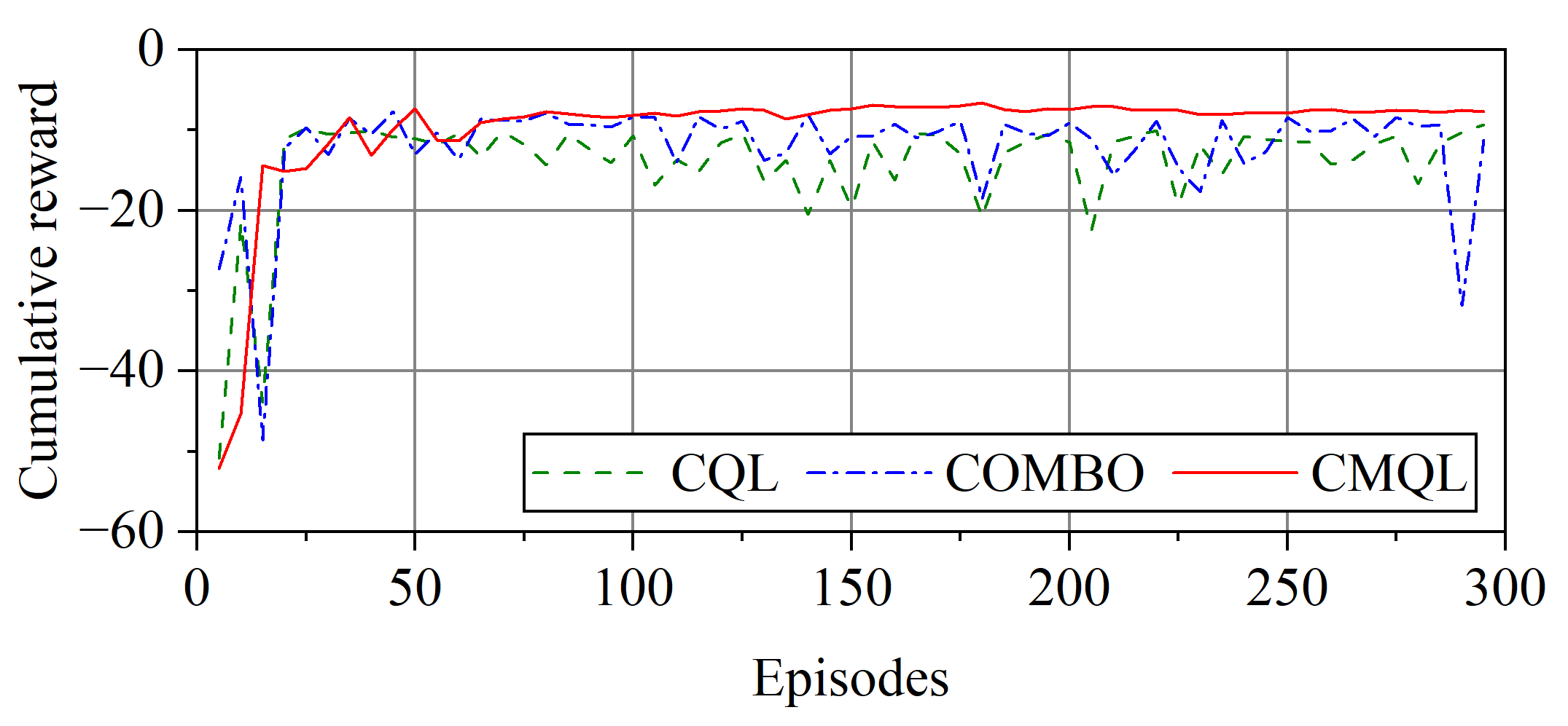
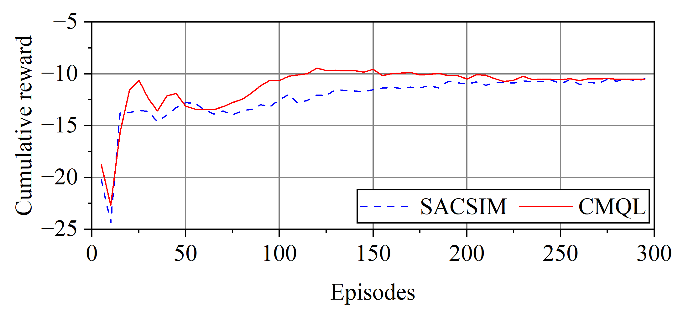
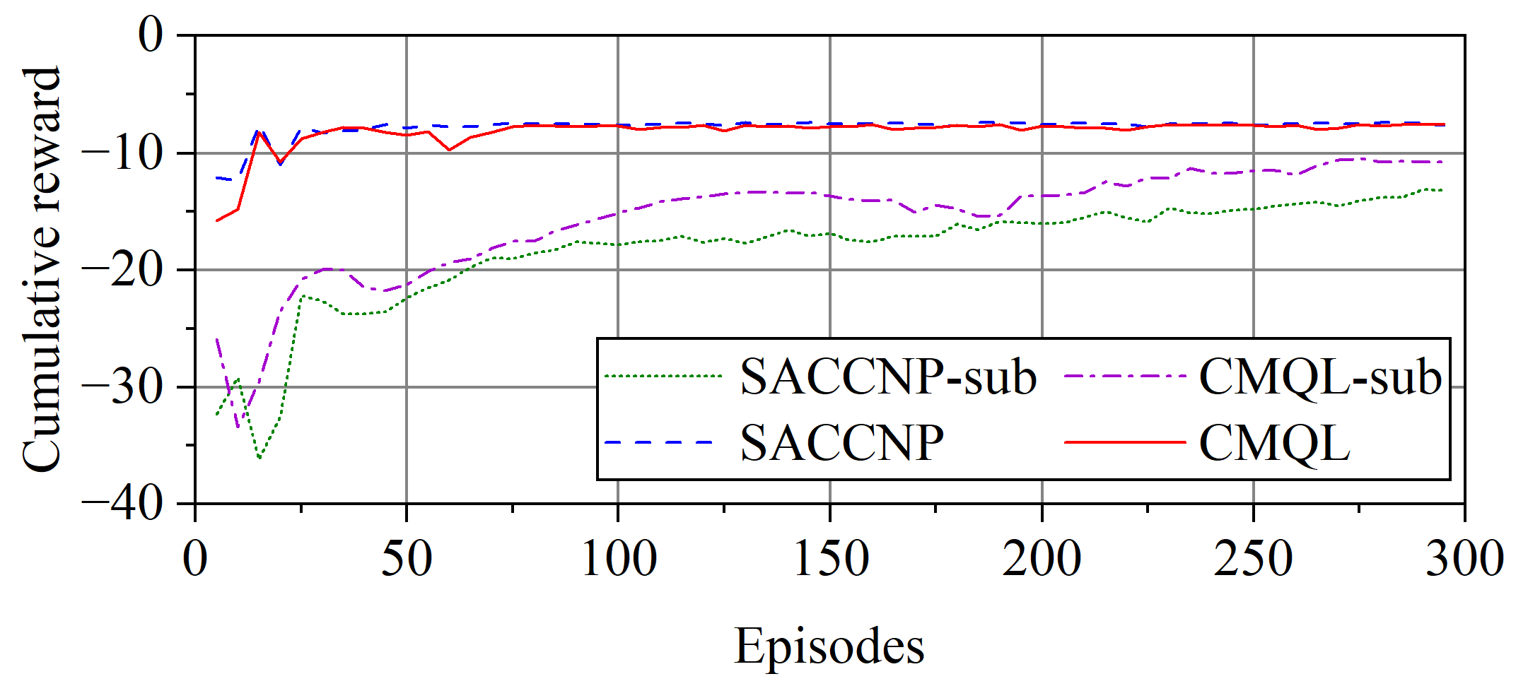
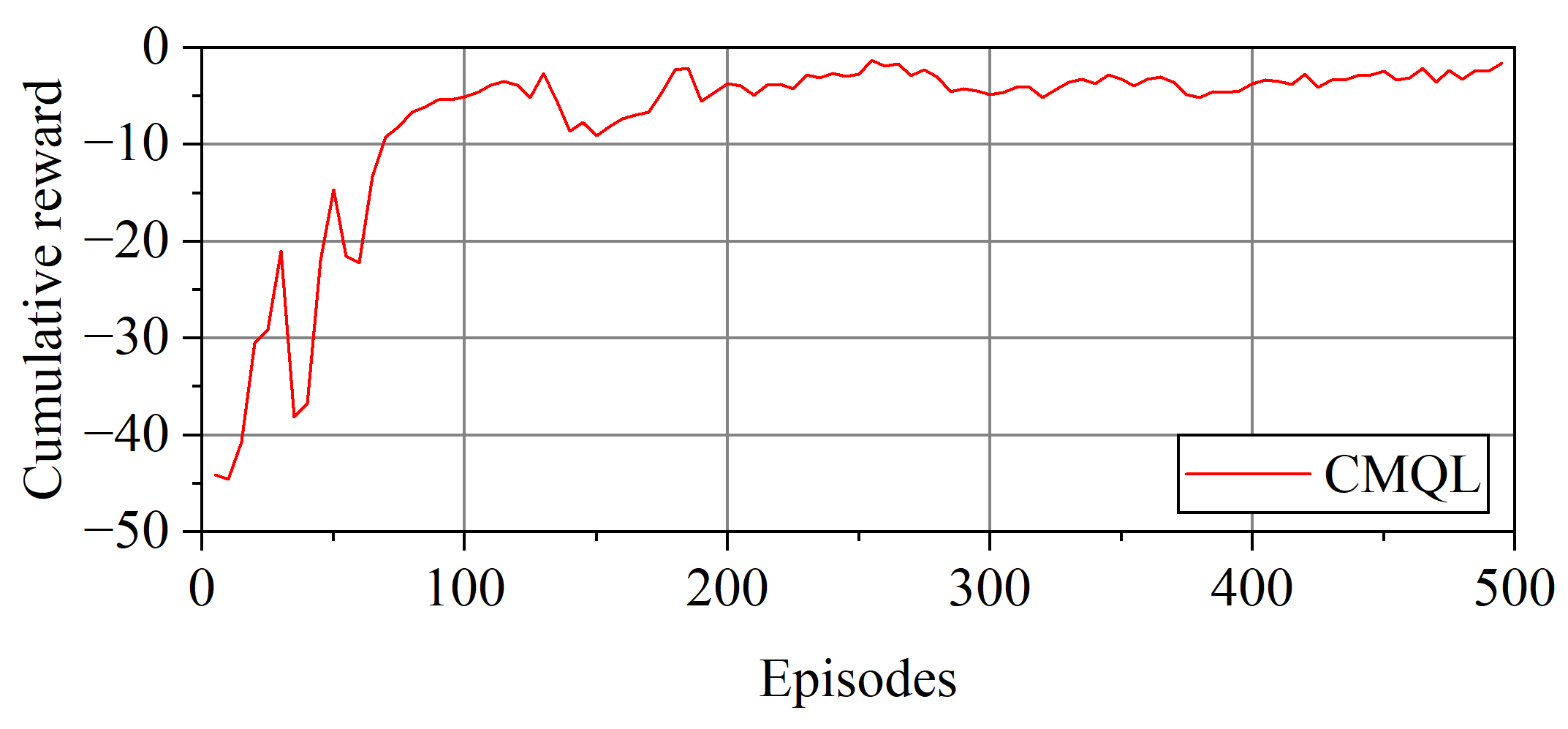
Figure 9.
Cumulative reward curve of surge velocity controllers.
Figure 9.
Cumulative reward curve of surge velocity controllers.
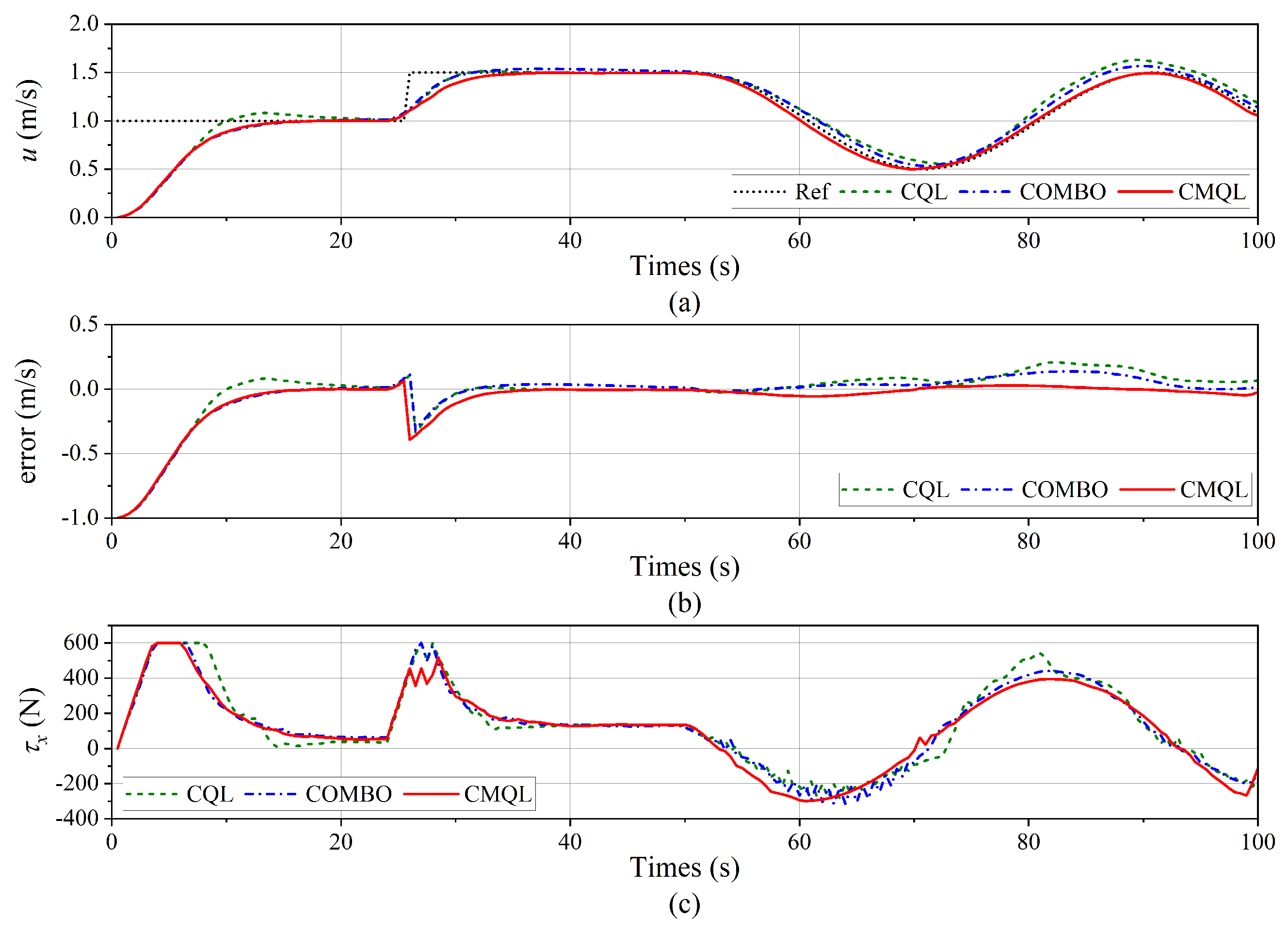
Figure 10.
Tracking result of the surge velocity control. (a) Surge velocity tracking curve. (b) Tracking error. (c) Propeller thrust.
Figure 10.
Tracking result of the surge velocity control. (a) Surge velocity tracking curve. (b) Tracking error. (c) Propeller thrust.
Figure 11.
Cumulative reward curve of the yaw velocity controllers.
Figure 11.
Cumulative reward curve of the yaw velocity controllers.
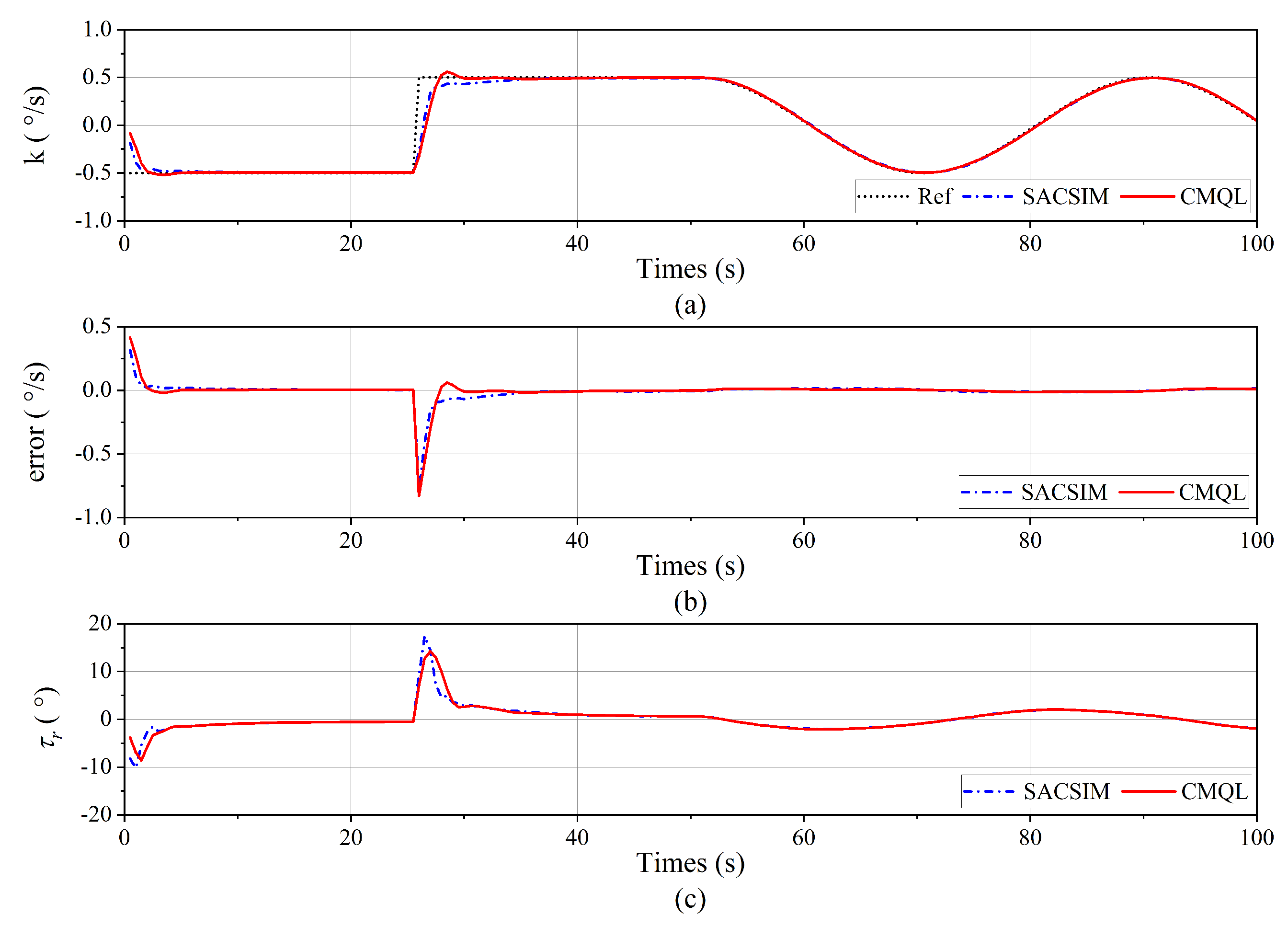
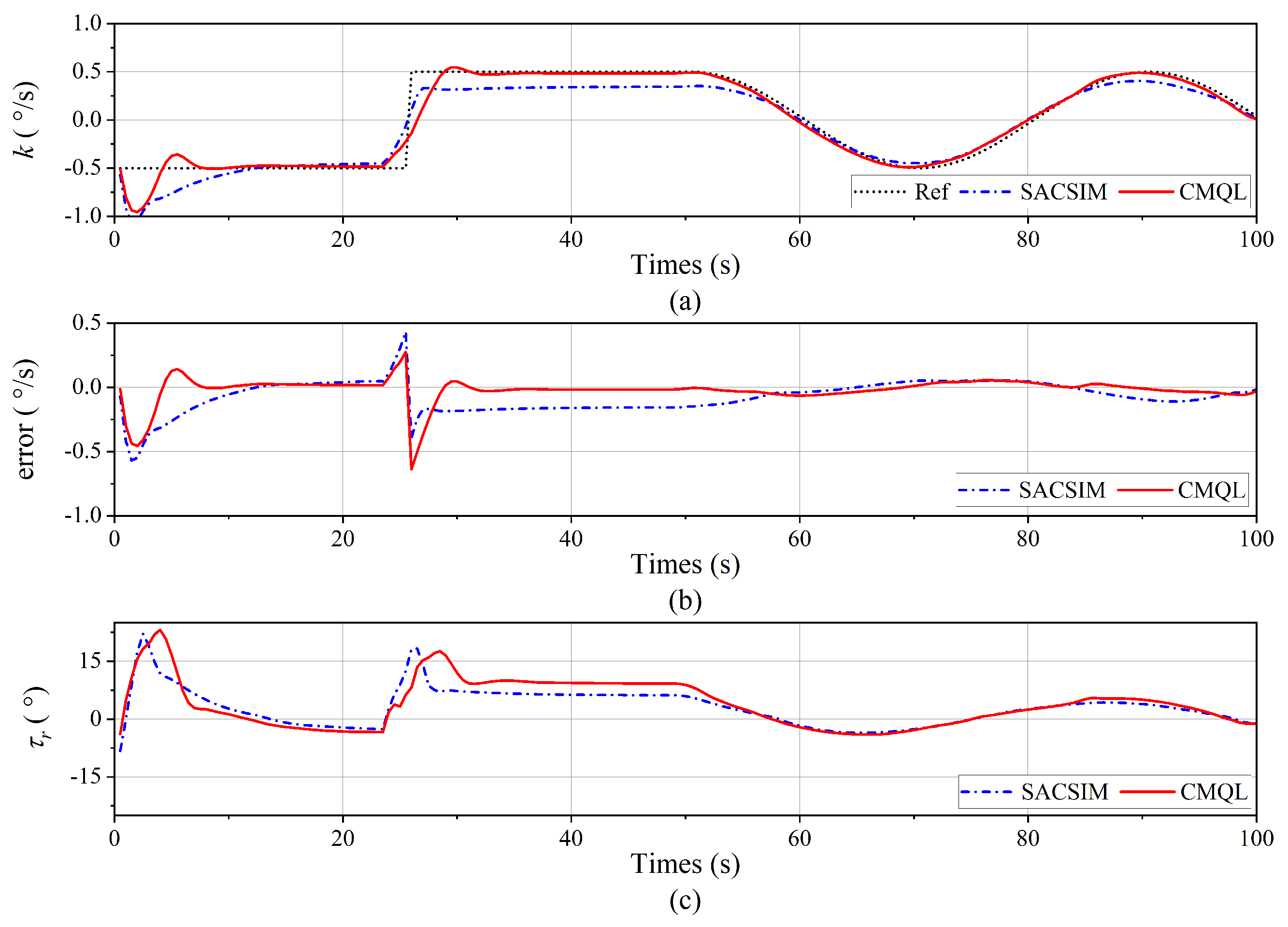
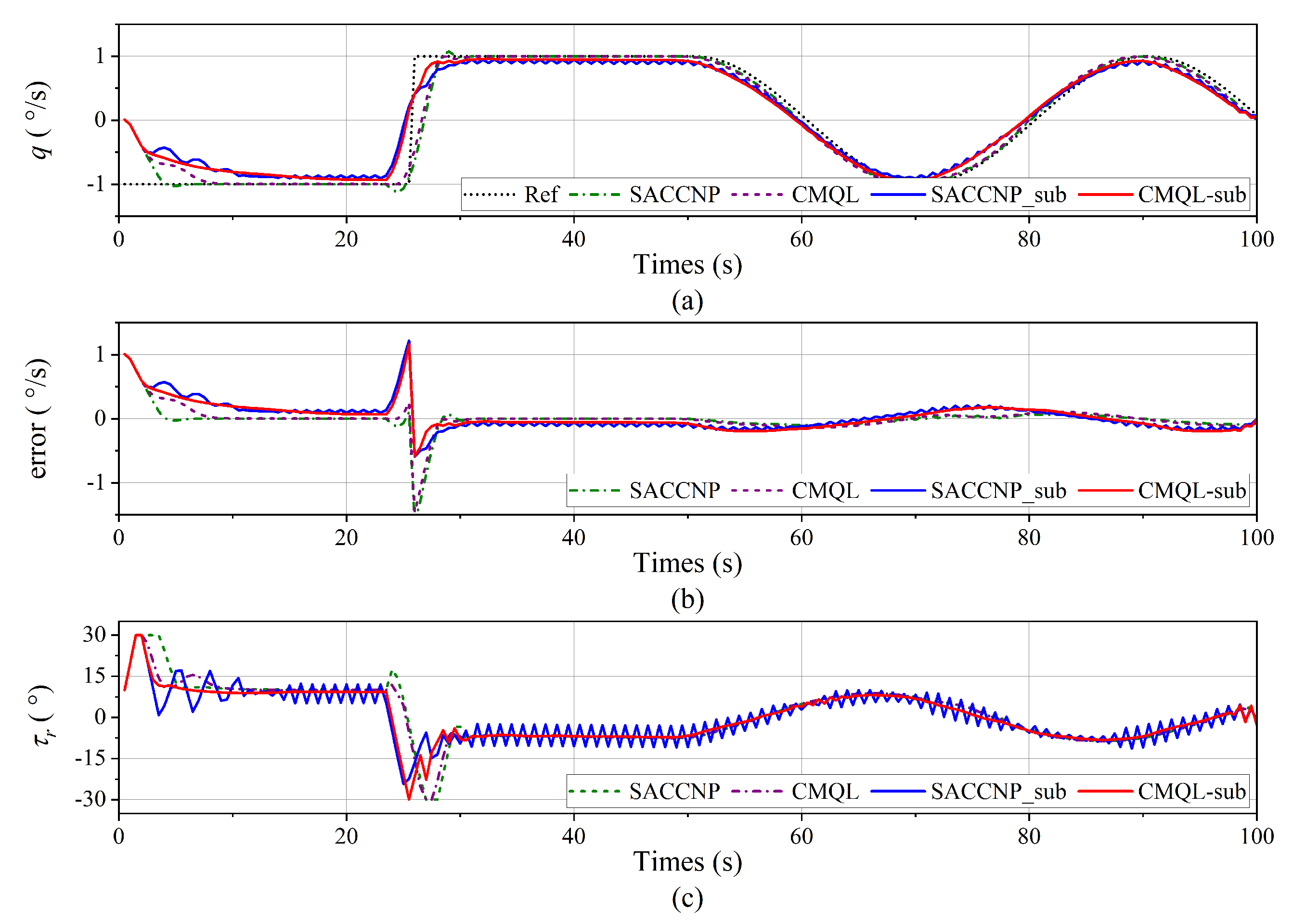
Figure 12.
Yaw velocity tracking result of the yaw velocity control without disturbance. (a) Yaw velocity tracking curve. (b) Tracking error. (c) Vertical rudder angle.
Figure 12.
Yaw velocity tracking result of the yaw velocity control without disturbance. (a) Yaw velocity tracking curve. (b) Tracking error. (c) Vertical rudder angle.
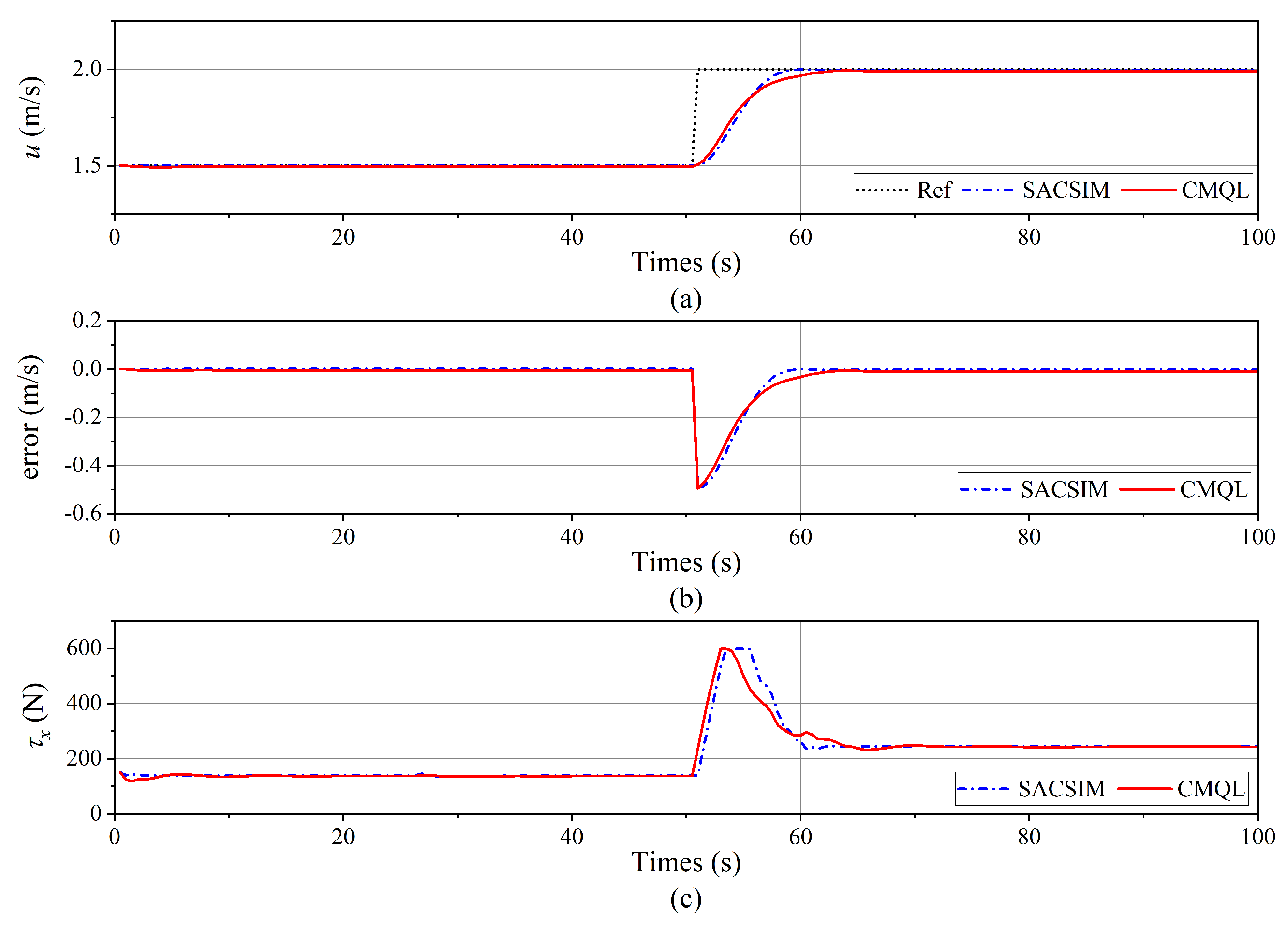
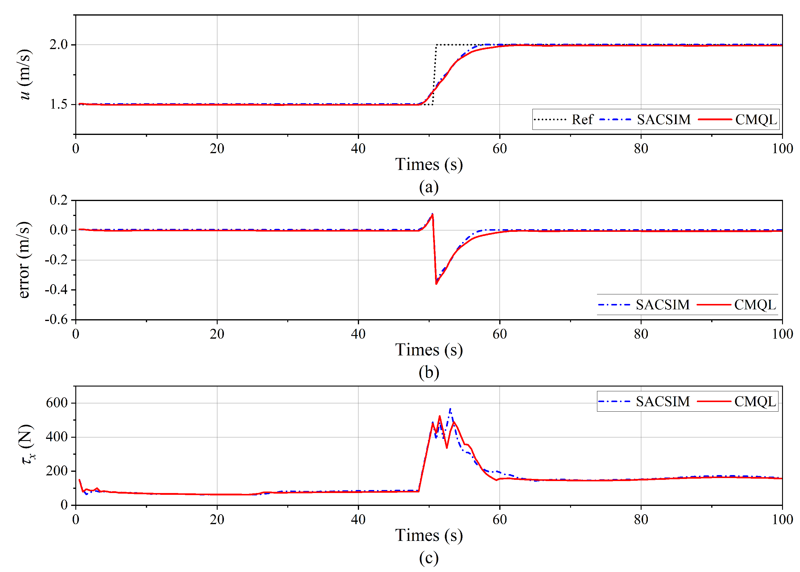
Figure 13.
Surge velocity tracking result of the yaw velocity control without disturbance. (a) Surge velocity tracking curve. (b) Tracking error. (c) Propeller thrust.
Figure 13.
Surge velocity tracking result of the yaw velocity control without disturbance. (a) Surge velocity tracking curve. (b) Tracking error. (c) Propeller thrust.
Figure 14.
Yaw velocity tracking result of the yaw velocity control under ocean current disturbance. (a) Yaw velocity tracking curve. (b) Tracking error. (c) Vertical rudder angle.
Figure 14.
Yaw velocity tracking result of the yaw velocity control under ocean current disturbance. (a) Yaw velocity tracking curve. (b) Tracking error. (c) Vertical rudder angle.
Figure 15.
Surge velocity tracking result of the yaw velocity control under ocean current disturbance. (a) Surge velocity tracking curve. (b) Tracking error. (c) Propeller thrust.
Figure 15.
Surge velocity tracking result of the yaw velocity control under ocean current disturbance. (a) Surge velocity tracking curve. (b) Tracking error. (c) Propeller thrust.
Figure 16.
Cumulative reward curve of the pitch velocity controllers.
Figure 16.
Cumulative reward curve of the pitch velocity controllers.
Figure 17.
Pitch velocity tracking result of the pitch velocity control. (a) Pitch velocity tracking curve. (b) Tracking error. (c) Horizontal rudder angle.
Figure 17.
Pitch velocity tracking result of the pitch velocity control. (a) Pitch velocity tracking curve. (b) Tracking error. (c) Horizontal rudder angle.
Figure 18.
Cumulative reward curve of the path-following controller.
Figure 18.
Cumulative reward curve of the path-following controller.
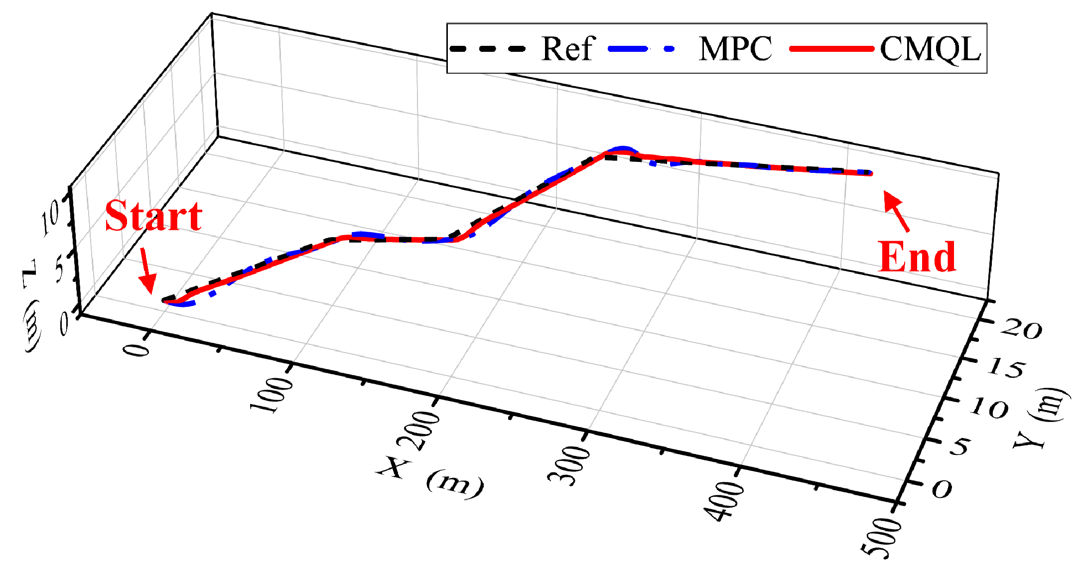
Figure 19.
AUV trajectory of the polyline path-following mission without disturbance.
Figure 19.
AUV trajectory of the polyline path-following mission without disturbance.
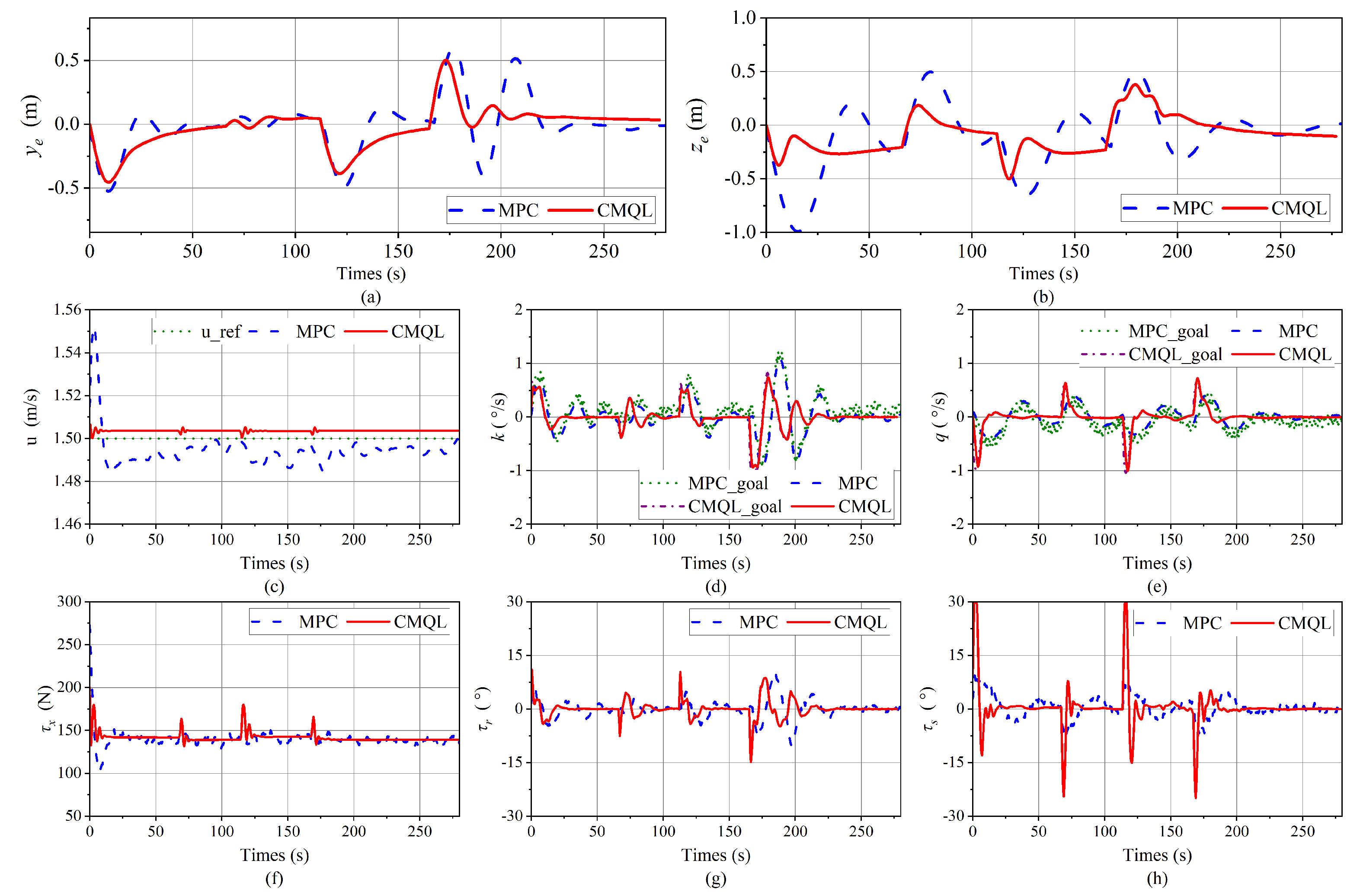
Figure 20.
Simulation results of the polyline path-following mission without disturbance. (a,b) Path-following errors. (c) Tracking results of the surge velocity. (d,e) Tracking results of velocity controllers. The outputs, CMQL_goal and MPC_goal, from the path-following controllers based on CMQL and MPC, are, respectively, employed as inputs to the corresponding velocity controllers. (f) Propeller thrust. (g) Vertical rudder angle. (h) Horizontal rudder angle.
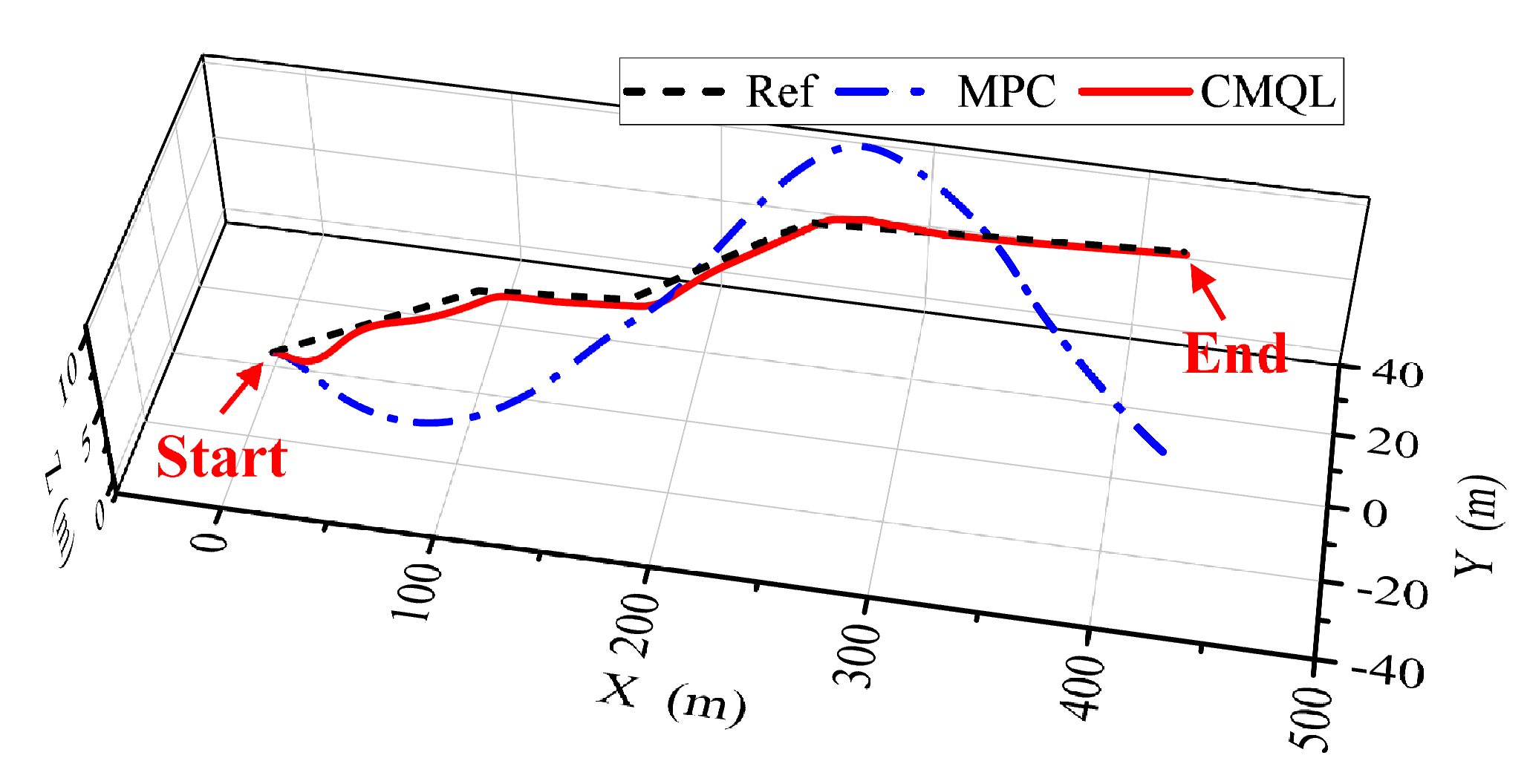
Figure 21.
AUV trajectory of the polyline path-following mission under ocean current disturbance.
Figure 21.
AUV trajectory of the polyline path-following mission under ocean current disturbance.
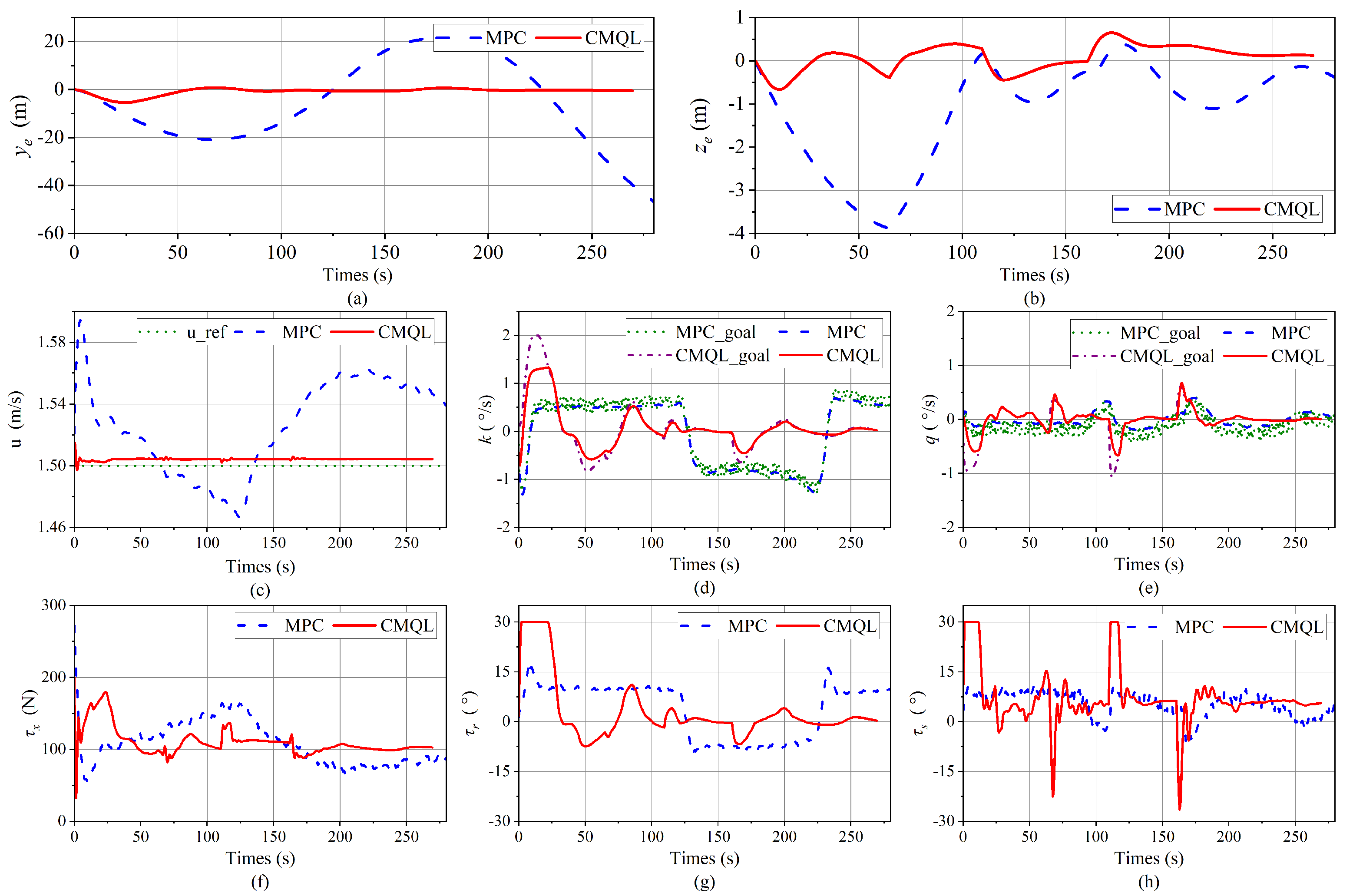
Figure 22.
Simulation results of the polyline path-following mission under ocean current disturbance. (a,b) Path-following errors. (c) Tracking results of the surge velocity. (d,e) Tracking results of velocity controllers. The outputs, CMQL_goal and MPC_goal, from the path-following controllers based on CMQL and MPC, are, respectively, employed as inputs to the corresponding velocity controllers. (f) Propeller thrust. (g) Vertical rudder angle. (h) Horizontal rudder angle.
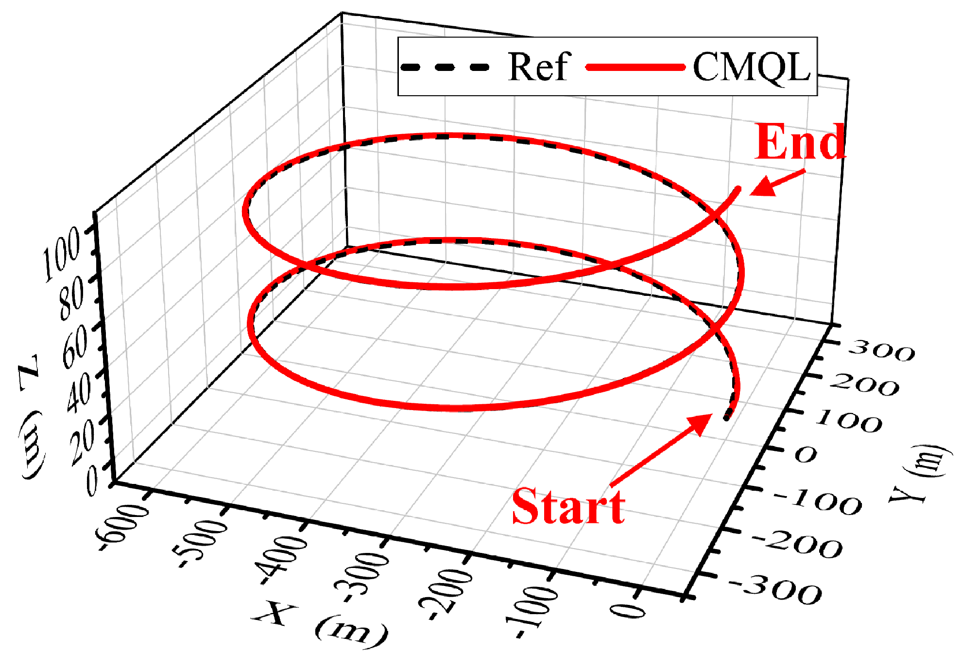
Figure 23.
AUV trajectory of the spiral path-following mission under variable ocean current disturbance.
Figure 23.
AUV trajectory of the spiral path-following mission under variable ocean current disturbance.
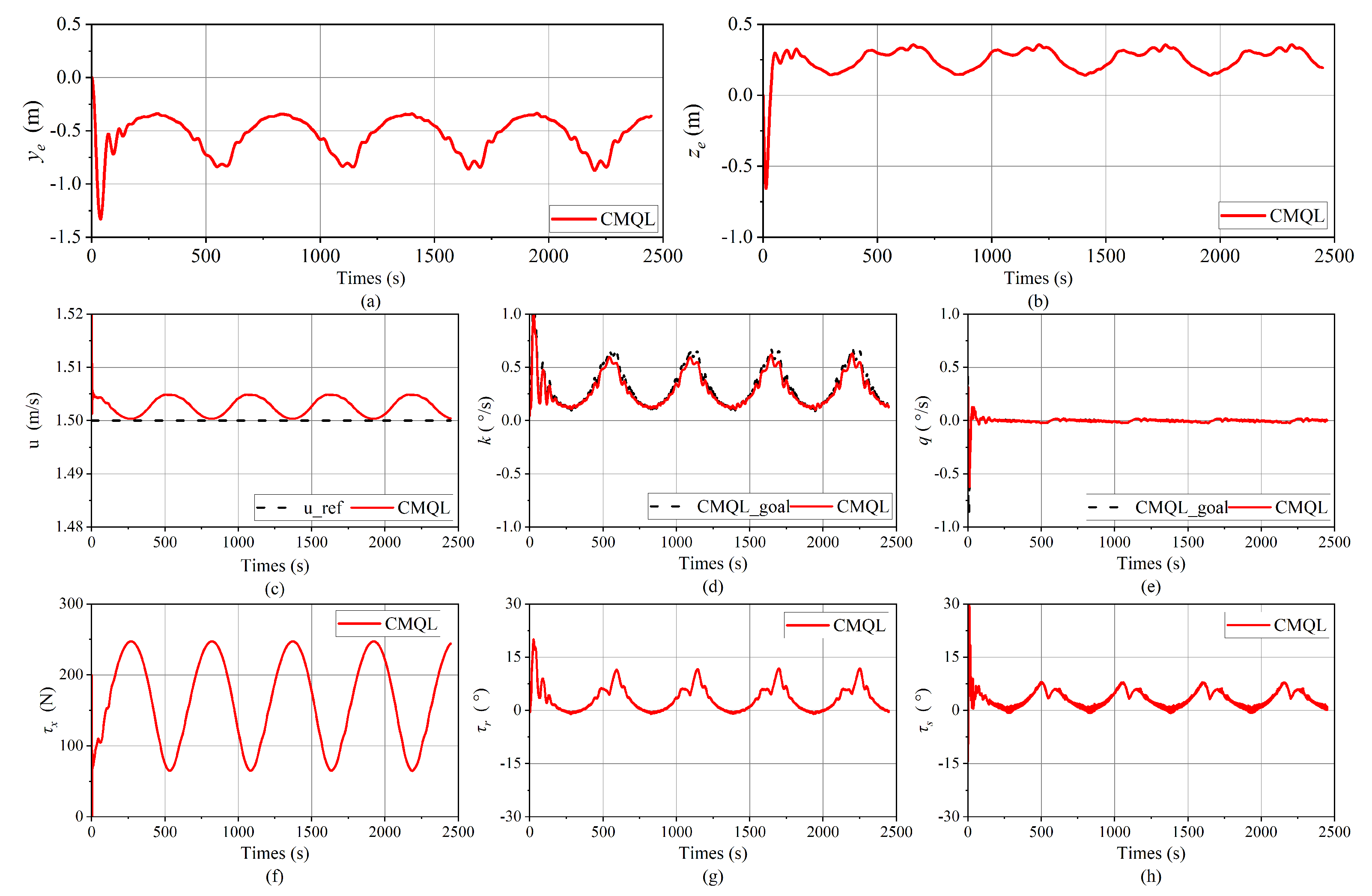
Figure 24.
Simulation results of the spiral path-following mission under variable ocean current disturbance. (a,b) Path-following errors. (c) Tracking results of the surge velocity. (d,e) Tracking results of velocity controllers. The outputs, CMQL_goal, from the path-following controller based on CMQL, are employed as inputs to the corresponding velocity controllers. (f) Propeller thrust. (g) Vertical rudder angle. (h) Horizontal rudder angle.
Table 1.
The performance evaluation for the CNP-based dynamics and kinematics models.
Table 1.
The performance evaluation for the CNP-based dynamics and kinematics models.
| | | | | u | q | k |
|---|
| 0.9811 | 0.9734 | 0.9926 | 0.9933 | 0.9911 | 0.9952 |
Table 2.
The performance indexes for the surge velocity control.
Table 2.
The performance indexes for the surge velocity control.
| | Setting Time (s) | Mean Error (m/s) | Max Error (m/s) |
|---|
| | 0 s∼25 s | 25 s∼50 s | 0 s∼25 s | 25 s∼50 s | 50 s∼100 s |
|---|
| CQL | 12 | 6 | 0.045 | −0.002 | 0.081 |
| COMBO | 10 | 6 | 0.001 | 0.026 | 0.051 |
| CMQL | 10 | 10 | −0.003 | −0.005 | −0.012 |
Table 3.
The yaw velocity tracking performance indexes for the yaw velocity control.
Table 3.
The yaw velocity tracking performance indexes for the yaw velocity control.
| | Ocean Current (m/s) | Setting Time (s) | Mean Error (°/s) | Max Error (°/s) |
|---|
| | | 0 s∼25 s | 25 s∼50 s | 0 s∼25 s | 25 s∼50 s | 50 s∼100 s |
|---|
| SACSIM | | 2 | 10 | 0.007 | −0.009 | 0.002 |
| 14 | 2 | 0.035 | −0.162 | −0.027 |
| CMQL | | 2.5 | 4 | 0.003 | −0.007 | 0.001 |
| 7 | 6 | 0.018 | −0.018 | −0.009 |
Table 4.
The surge velocity tracking performance indexes for the yaw velocity control.
Table 4.
The surge velocity tracking performance indexes for the yaw velocity control.
| | Ocean Current (m/s) | Setting Time (s) | Mean Error (°/s) |
|---|
| | | 50 s∼100 s | 0 s∼50 s | 50 s∼100 s |
|---|
| SACSIM | | 8 | 0.002 | −0.003 |
| 6 | 0.004 | 0.002 |
| CMQL | | 12 | −0.005 | −0.01 |
| 10 | −0.002 | −0.006 |
Table 5.
The performance indexes for the pitch velocity control.
Table 5.
The performance indexes for the pitch velocity control.
| | Setting Time (s) | Mean Error (°/s) | Max Error (°/s) |
|---|
| | 0 s∼25 s | 25 s∼50 s | 0 s∼25 s | 25 s∼50 s | 50 s∼100 s |
|---|
| SACCNP | 6 | 5.5 | −0.004 | −0.001 | −0.113 |
| CMQL | 9 | 5 | 0.005 | −0.003 | −0.132 |
| SACCNP-sub | 12 | 5 | 0.126 | −0.086 | 0.210 |
| CMQL-sub | 13 | 5 | 0.102 | −0.054 | −0.173 |
Table 6.
The performance indexes for polyline path-following mission.
Table 6.
The performance indexes for polyline path-following mission.
| | Ocean Current (m/s) | Mean Error (m) | Max Error (m) | Completion |
|---|
| | | | | | |
Time (s)
|
|---|
| MPC | | 0.010 | −0.103 | 0.598 | −0.992 | 281.5 |
| −5.972 | −0.131 | −51.449 | −3.886 | 288 |
| CMQL | | −0.025 | −0.089 | 0.502 | −0.503 | 277 |
| −0.242 | −0.089 | −4.621 | −0.665 | 269.5 |
Table 7.
The performance indexes for spiral path-following mission under variable ocean current disturbance.
Table 7.
The performance indexes for spiral path-following mission under variable ocean current disturbance.
| | Mean Error (m) | Max Error (m) |
|---|
| | | | | |
|---|
| CMQL | −0.539 | 0.249 | −0.873 | 0.356 |


