Physics-Aware Machine Learning Approach for High-Precision Quadcopter Dynamics Modeling

Abstract

In this paper, we propose a physics-informed neural network controller for quadcopter dynamics modeling. Physics-aware machine learning methods, such as physics-informed neural networks, consider the UAV dynamics model, solving the system of ordinary differential equations entirely, unlike proportional–integral–derivative controllers. The more accurate control action on the quadcopter reduces flight time and power consumption. We applied our fractional optimization algorithms to decreasing the solution error of quadcopter dynamics. Including advanced optimizers in the reinforcement learning model, we achieved the trajectory of UAV flight more accurately than state-of-the-art proportional–integral–derivative controllers. The advanced optimizers allowed the proposed controller to increase the quality of the building trajectory of the UAV compared to the state-of-the-art approach by 10 percentage points. Our model had less error value in spatial coordinates and Euler angles by 25–35% and 30–44%, respectively.

1. Introduction

Unmanned aerial vehicles [1] (UAVs) are a necessary part of modern scientific and industrial human activities. Due to such technologies, many researchers have achieved valuable and advanced results in logistics [2], digital agriculture [3], geoprospecting [4], and other areas of human activity. The explosive growth of UAV integration in civil applications requires advanced and modified control algorithms, which preserve the quality and stability of computations for facilitating real-world deployment. In addition to their UAV application, control systems have acquired new high-precision approaches, especially self-learning. In recent decades, model-based control (MBC) systems [5] have been applied in many scientific and industrial areas. Thanks to their powerful approximation properties, such techniques increase the quality of UAV dynamics modeling. The most dispersed MBC is the proportional–integral–derivative (PID) [6] method. This approach analyzes error via the summation of proportion, integral, and derivative terms. This approach has been providing required quality and accuracy since the year 2016. In [7], the authors provided various modifications, such as being adaptive, event-based, gain-scheduling, fault-tolerant, and one of the most advanced fractional. Among the state-of-the-art (SOTA) MBCs, there exist other approaches: linear quadratic regulator (LQR) [8], linear quadratic Gaussian (LQG) [9], and soft actor–critic (SAC) [10]. However, as these technologies belong to MBC systems, they are less adaptive than data-driven (DD) [11] models.

The authors in [12] proposed a nonlinear control model with backstepping control for quadrotor dynamics simulation. As a helpful enhancement, the researchers in [13] suggested synthesized sliding-mode control for quadcopter dynamics modeling. In [14], the developers created a control strategy to improve the energy efficiency of a quadrotor for field inspections. In paper [15], the authors proposed geometric adaptive control, which is based on a neural network. This model design was based directly on the special Euclidean group, to avoid the complexities of singularities inherent to local parameterizations. In [16], the authors developed the quantized fuzzy feedback control for electric vehicle lateral dynamics. However, this approach did not consider the physical properties of UAV flight, which could have raised the quality of drone predictive control. Thus, we propose a physics-informed neural network for quadcopter flight dynamics modeling. The first DD method was proximal policy optimization (PPO) [17], based on policy gradient descent. Unfortunately, this DD model consists of an outdated optimizer and multilayer perceptron (MLP) [18] neural network model. As an alternative, the researchers in [19] used physics-aware machine learning models, such as physics-informed neural networks (PINNs). This DD model considers the mathematical model of UAV flight dynamics, considering its positions, velocities, accelerations, and angular parameters. Next, a PINN solves the system of differential equations and achieves more accurate results than MBC approaches. Like other neural networks, a PINN consists of input, hidden layers, output, and backpropagation. To minimize the loss function, many researchers use either stochastic gradient descent (SGD) or adaptive moment estimation (Adam) [20]. These optimization algorithms are first-order and are appropriate in neural networks, solving pattern recognition, time series prediction, and object detection.

1.1. Motivation

The main problem in modeling quadcopter dynamics is building a trajectory between the checkpoints that has the required accuracy and performance. The most common solution to this problem is a PID-based controller application. However, the MBC method is less adaptive than DD techniques. The fractional proportional–integral–derivative (FOPID) is a modification that locally improves modeling. These MBC approaches were reinforced in [21] by the Runge–Kutta numerical method for solving the differential equation systems. Traditional numerical methods build the approximate solution by sequent points. As an alternative numerical method, many researchers use physics-aware machine learning models. Unlike the usual numerical methods, self-learning algorithms build the approximate solution by epochs, analyzing it entirely. The automatic differentiation layer considers differential equations and additional conditions. Moreover, such an approach is universal. A PINN can be edited under integral, fractional, delay, and functional equations with corresponding conditions [22,23]. In many manuscripts, PINN-based approaches have allowed for modeling quadcopter flight trajectories with higher accuracy and performance. Unlike PID and FOPID, a PINN builds a trajectory by using a self-learning algorithm, such as backpropagation. The main feature of this DD model is backpropagation, correcting weights in hidden layers to improve the next output. This method is reinforced by loss function minimization via first-order optimizers SGD [20] and Adam [24]. They have many modifications, such as DiffGrad, Yogi, AdaBelief, AdaBound, and other gradient-based first-order analogs. These optimizers can achieve the global minimum of loss function for many iterations (epochs). This fact can be seen in experiments on test function minimization. Replacing SOTA optimizers with second-order (quasi-Newton) approaches [25], AdaHessian and Apollo, causes rising computational costs. Therefore, one needs to apply alternative optimization algorithms, such as fractional. The application of fractional derivatives in physics-informed neural networks is justified by their more profound analysis of loss function than conventional approaches, such as SGD and Adam. The set fractional integral and derivatives are divided into four classes: classical, modified, local operator, and non-singular kernel operators. The Riemann–Liouville, Caputo, and Grunwald–Letnikov fractional derivatives belong to the classical subset, which can be identified by their similar Taylor series expansions. We chose these derivatives because of their adaptability under conventional backpropagation in neural networks. Modified (Weyl, Marchaud, Hadamard, Erdélyi–Kober, Tarasov), local operators (Kolwankar, Chen, Conformable, Katugampola), and operators with the non-singular kernel (Caputo–Fabrizio, Atangana–Baleanu Caputo, Atangana–Baleanu, Riemann–Liouville, Sun Hao Zhang–Baleanu) derivatives have a complex definition, the approximation of which will not achieve the physics-aware learning requirements. In [26], we developed fractional gradient descent with Riemann–Liouville, Caputo, and Grunwald–Letnikov derivatives. This optimizer demonstrated better results in test function minimization and pattern recognition solving using a Swin transformer. Considering the manuscripts [27], we expressed the approximate fractional gradient calculations and attained the compatible computational costs with minimal loss of accuracy. The fractional optimizers provided had the compatibility for neural network training convergence rate and stability, $O\left(\sqrt{T}\right)$ and $O\left(T\right)$, respectively. Utilizing fractional optimizers in PINN-based controllers can improve quadcopter dynamics modeling. If the quadcopter attains checkpoints faster then it consumes less power. Such an improvement allows for increasing the quality of service of power lines [28], logistics [3], agriculture [29], and remote sensing [30]. Moreover, DD modeling is a growing industrial area where many tools can be advanced.

1.2. Our Contribution

The main contributions of our investigation are summarized as follows:

(i) We propose a novel fractional physics-informed neural network with Riemann–Liouville, Caputo, and Grunwald–Letnikov derivatives for solving quadcopter dynamics problems.

(ii) We include the proposed fractional physics-informed neural network in a quadcopter controller. Due to its self-learning property, the proposed approach achieves its results with fewer positional and angular errors than the SOTA.

(iii) The proposed approach allows quadcopter flight modeling, consuming less time than the SOTA. This advantage lets the quadcopter consume less power.

The novelty of the proposed AI-based controller of a quadcopter is the integration of fractional-order optimization algorithms in physics-informed neural network training. Many physics-aware machine learning models are based on conventional stochastic gradient descent and adaptive moment estimation, reinforcing the minimization process via second-order optimization algorithms via L-BFGS. Such a technique allows us to achieve the solution with the required accuracy, but time consumption increases. Our fractional optimizer with Riemann–Liouville, Caputo, and Grunwald–Letnikov derivatives does not require an additional minimizer, like L-BFGS [31] or SR-1 [32], because it can converge to the global minimum loss function neighborhood for fewer epochs. This happens because of a more generalized analysis of the loss function surface. We fill the physics-informed controller of the quadcopter with this advanced optimizer, which allows us to increase the final accuracy of the UAV control.

1.3. Structure of the Paper

The rest of this article is organized in the following structure. Section 2 shows the SOTA for the mathematical model of quadcopter dynamics, a proportional–integral–derivative controller, and a fractional optimization algorithm with Riemannian–Liouvile, Caputo, Grunwald–Letnikov derivatives. Section 3 is devoted to the proposed fractional physics-informed neural network controller for solving quadcopter dynamics problems. Section 4 contains the experiments for building the flight trajectory of a quadcopter by the SOTA and the proposed methods. Section 5 contains possible ways to improve and modify the proposed fractional physics-informed neural networks and the available application areas. In Section 6, we draw conclusions about the proposed controller and its further applications.

2. State-of-the-Art in Quadcopter Dynamics Modeling

2.1. Mathematical Model of Quadcopter Dynamics

The mathematical model of quadcopter flight follows the basic rules of applied mechanics [27]. The quadrotor’s position is defined via $(x,y,z)$, Euler angles (roll, pitch, and yaw angles) $(\varphi ,\theta ,\psi )$, $\varphi \in [-\pi /2,\pi /2]$, $\theta \in (-\pi /2,\pi /2)$, and $\psi \in [-\pi ,\pi )$. The parameters $v=(\dot{x},\dot{y},\dot{z})$ and $\omega =({\omega }_1,{\omega }_2,{\omega }_3)$ are the linear and angular velocities of the quadcopter center of mass, respectively. The quadcopter flight dynamics can be described by the following formulas:

$$\dot{v}={\displaystyle \frac{1}{m}}(f+f_g),$$

(1)

$$\left[\begin{array}{c}\dot{\varphi }\\ \dot{\theta }\\ \dot{\psi }\end{array}\right]=M\left(\left[\begin{array}{c}\varphi \\ \theta \\ \psi \end{array}\right]\right)\omega ,$$

(2)

$$\dot{\omega }=J^{-1}(-\widehat{\omega }J\omega +\tau +{\tau }^{\prime }),$$

(3)

where m is the quadcopter mass, $f=R\left({[\varphi ,\theta ,\psi ]}^T\right){\varphi }_p$ denotes the propeller force, J is the quadcopter inertia matrix, and

$$\widehat{\omega }=\left[\begin{array}{ccc}0& -{\omega }_3& {\omega }_2\\ {\omega }_3& 0& -{\omega }_1\\ -{\omega }_2& {\omega }_1& 0\end{array}\right]$$

(4)

is the so-called dyadic representation of $\omega$. Furthermore, the input forces and moments generated by the propellers can be expressed via the following forms:

$${\varphi }_p=\left[\begin{array}{c}0\\ 0\\ u_p\end{array}\right],u_p=\sum _{i=1}^4{f}_i,f_g=\left[\begin{array}{c}0\\ 0\\ -mg\end{array}\right],$$

(5)

$${\tau }_p=\left[\begin{array}{c}{\tau }_1\\ {\tau }_2\\ {\tau }_3\end{array}\right]=\left[\begin{array}{c}lb({\omega }_{p,2}^2-{\omega }_{p,4}^2)\\ lb({\omega }_{p,3}^2-{\omega }_{p,2}^2)\\ c({\omega }_{p,1}^2-{\omega }_{p,2}^2+{\omega }_{p,3}^2-{\omega }_{p,4}^2)\end{array}\right]$$

(6)

where l is the distance from the center of mass to the motor shaft, and where b and c are the thrust and drag coefficient, respectively; $f_g$ is the gravitational force, and

$$R\left(\left[\begin{array}{c}\varphi \\ \theta \\ \psi \end{array}\right]\right)=\left[\begin{array}{ccc}{c}_{\theta }{c}_{\psi }& s_{\varphi }{s}_{\theta }{c}_{\psi }-c_{\varphi }{s}_{\psi }& c_{\varphi }{s}_{\theta }{c}_{\psi }+s_{\varphi }{s}_{\psi }\\ c_{\theta }{s}_{\psi }& s_{\varphi }{s}_{\theta }{s}_{\psi }+c_{\varphi }{c}_{\psi }& c_{\varphi }{s}_{\theta }{s}_{\psi }-s_{\varphi }{c}_{\psi }\\ -s_{\theta }& s_{\varphi }{c}_{\theta }& c_{\varphi }{c}_{\theta }\end{array}\right],$$

(7)

$$M\left(\left[\begin{array}{c}\varphi \\ \theta \\ \psi \end{array}\right]\right)=\left[\begin{array}{ccc}1& s_{\varphi }{t}_{\theta }& c_{\varphi }{t}_{\theta }\\ 0& c_{\varphi }& -s_{\varphi }\\ 0& s_{\varphi }sec\left(\theta \right)& c_{\varphi }sec\left(\theta \right)\end{array}\right],$$

(8)

where $c_{*}=\cos (\ast )$, $s_{*}=\sin (\ast )$, and $t=\tan (\ast )$ with $*=\varphi ,\theta ,\psi$. If we suppose that $\varphi$ and $\theta$ are small angles, which means non-aggressive maneuvers of the quadcopter, then matrix (11) will be approximately equal to the identity matrix. Considering Newton’s third law, the propellers exert a yawing torque ${\tau }_3$ on the quadrotor body in the direction opposite to the propeller rotation. Next, one can see that

$$\left[\begin{array}{c}{f}_1\\ f_2\\ f_3\\ f_4\end{array}\right]={\left[\begin{array}{cccc}1& 1& 1& 1\\ 0& l& 0& l\\ -l& 0& l& 0\\ c& -c& c& -c\end{array}\right]}^{-1}=\left[\begin{array}{c}{u}_p\\ {\tau }_1\\ {\tau }_2\\ {\tau }_3\end{array}\right],$$

(9)

$$\left[\begin{array}{c}{\omega }_{p,1}^2\\ {\omega }_{p,2}^2\\ {\omega }_{p,3}^2\\ {\omega }_{p,4}^2\end{array}\right]=\left[\begin{array}{cccc}{\displaystyle \frac{1}{4b}}& 0& -{\displaystyle \frac{1}{2bl}}& {\displaystyle \frac{1}{4c}}\\ {\displaystyle \frac{1}{4b}}& {\displaystyle \frac{1}{2bl}}& 0& -{\displaystyle \frac{1}{4c}}\\ {\displaystyle \frac{1}{4b}}& 0& {\displaystyle \frac{1}{2bl}}& {\displaystyle \frac{1}{4c}}\\ {\displaystyle \frac{1}{4b}}& -{\displaystyle \frac{1}{2bl}}& 0& -{\displaystyle \frac{1}{4c}}\end{array}\right]=\left[\begin{array}{c}{u}_p\\ {\tau }_1\\ {\tau }_2\\ {\tau }_3\end{array}\right],$$

(10)

$${\omega }_{p,i}=\sqrt{{\displaystyle \frac{f_i}{b}}},0\le f_i\le f_{i,max},0\le {\omega }_{p,i}\le {\omega }_{p,i,max}$$

(11)

where $f_{i,max}$ and ${\omega }_{p,i,max}$, for $i=1,2,3,4$, denote the maximum forces and angular velocities for each propeller, constrained by physical limitations. Furthermore, the gyroscopic torque arising from the propeller rotations is given by

$${\tau }^{\prime }=\sum _{i=1}^4{(-1)}^i{J}_{p,i}{\omega }_{p,i}\widehat{\omega }{\widehat{ϵ}}_3$$

(12)

where $J_{p,i}$, for $i=1,2,3,4$, is the moment of inertia of the i motor and propeller about its axis of rotation. The gyroscopic torque can be described by the following equalities:

$$\dot{x}\left(t\right)=v_x\left(t\right),\dot{y}\left(t\right)=v_y\left(t\right),\dot{z}\left(t\right)=v_z\left(t\right),$$

(13)

$${\dot{v}}_x\left(t\right)=\left(c_{\varphi \left(t\right)}{s}_{\theta \left(t\right)}{c}_{\psi \left(t\right)}+s_{\varphi \left(t\right)}{s}_{\psi \left(t\right)}\right){\displaystyle \frac{u_p\left(t\right)}{m}},$$

$${\dot{v}}_y\left(t\right)=\left(c_{\varphi \left(t\right)}{s}_{\theta \left(t\right)}{s}_{\psi \left(t\right)}+s_{\varphi \left(t\right)}{c}_{\psi \left(t\right)}\right){\displaystyle \frac{u_p\left(t\right)}{m}},$$

$${\dot{v}}_z\left(t\right)=-g+c_{\varphi \left(t\right)}{c}_{\theta \left(t\right)}{\displaystyle \frac{u_p\left(t\right)}{m}},$$

$$\dot{\varphi }\left(t\right)={\omega }_1\left(t\right),\dot{\theta }\left(t\right)={\omega }_2\left(t\right),\dot{\psi }\left(t\right)={\omega }_3\left(t\right),$$

$$\dot{{\omega }_1}\left(t\right)={\displaystyle \frac{J_2-J_3}{J_1}}{\omega }_2\left(t\right){\omega }_3\left(t\right)+{\displaystyle \frac{J_p}{J_1}}{\omega }_p\left(t\right){\omega }_2\left(t\right)+{\displaystyle \frac{1}{J_1}}{\tau }_1\left(t\right)$$

$$\dot{{\omega }_2}\left(t\right)={\displaystyle \frac{J_3-J_1}{J_2}}{\omega }_1\left(t\right){\omega }_3\left(t\right)-{\displaystyle \frac{J_p}{J_1}}{\omega }_p\left(t\right){\omega }_1\left(t\right)+{\displaystyle \frac{1}{J_1}}{\tau }_2\left(t\right)$$

$$\dot{{\omega }_1}\left(t\right)={\displaystyle \frac{J_1-J_2}{J_3}}{\omega }_1\left(t\right){\omega }_2\left(t\right)+{\displaystyle \frac{1}{J_3}}{\tau }_3\left(t\right).$$

Considering the provided UAV dynamics model, one can build a PID-based controller, which takes into account the above drone parameters for modeling the flight trajectory.

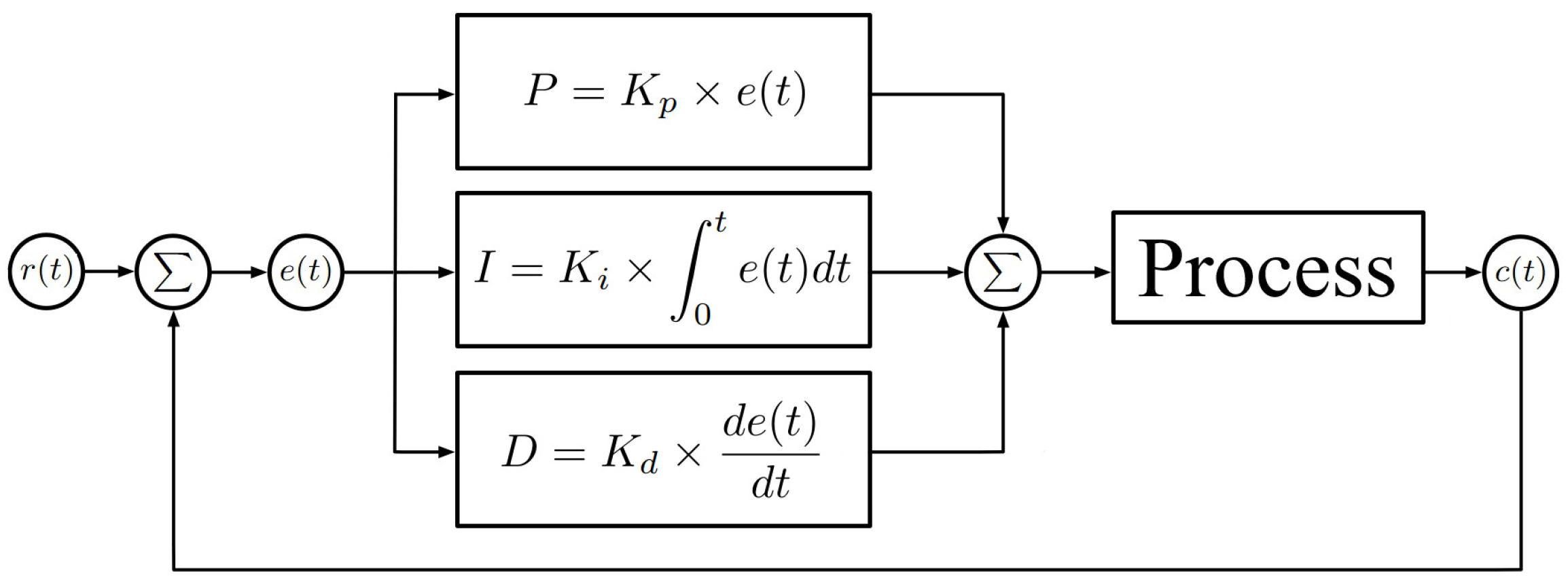
2.2. Proportional–Integral–Derivative Controller

PID-based controllers [6] are widely applied in robotics and autonomous systems. This method is the most dispersed and successful among the existing MBC analogs. PID-based controllers analyze the dynamical system in three directions, using usual, integral, and derivative. This allows us to consider not just regular variables, such as Cartesian, spherical, cylindrical, and many other positions, but also velocities and accelerations. This technique improves parameter corrections. Studies in stabilizing quadcopters and other UAV systems by PID control have been realized since 2004 [33].

A PID-based controller has many merits, including lowering the downtime, upward thrust time, and smoothing the motion. Meanwhile, this sort of controller has many problems with parameter adjustment. For example, its low capacity for tracking P, I, and D parameters might also bring about negative performance, gradual management, and, in a few cases, machine instability. Consequently, the great variety of tuning techniques for PID controllers calls for significant interest from the operator, to pick out the gold standard set of values for the parameters, to attain an inexpensive gain. However, in some cases, this approach no longer produces practical consequences in lowering the time response of the signal:

$$P=K_p\times e\left(t\right),I=K_i\times {\int }_0^{t}e\left(t\right)dt,D=K_d\times {\displaystyle \frac{de\left(t\right)}{dt}}.$$

The control function can be expressed mathematically as

$$u\left(t\right)=K_{p}e\left(t\right)+K_i{\int }_0^{t}e\left(t\right)dt+K_d{\displaystyle \frac{de\left(t\right)}{dt}}.$$

The more precise scheme of the PID controller is presented in Figure 1:

Such a PID approach works for integer order control systems, making the modeling process more simple with a fast response. However, the facility of the model does not guarantee implementation without artifacts (events with high error), which is met in UAV dynamics modeling. Note that the PID approach is designed for complex linear systems. In the case of quadcopter flight modeling, an adaptive PID-based controller is used for more accurate model tuning. For that reason, the author in [21] decided to utilize FOPID. This technique improves the model tuning via more adaptive integral and derivative structures. The mathematical expression of FOPID is

$$u\left(t\right)=K_{p}e\left(t\right)+K_i\times {}_{0}I_t^{\lambda }e\left(t\right){\left(dt\right)}^{\lambda }+K_d\times {}_{0}D_t^{\mu }e\left(t\right)$$

where

$${}_{0}I_t^{\lambda }e\left(t\right)={\displaystyle \frac{1}{\Gamma \left(\lambda \right)}}{\int }_0^t{\displaystyle \frac{e\left(\kappa \right)}{{(\kappa -t)}^{1-\lambda }}}d\kappa \mathrm{and}{D}_0^{\mu }e\left(t\right)={\displaystyle \frac{1}{\Gamma (1-\mu )}}{\displaystyle \frac{d}{dt}}{\int }_0^t{\displaystyle \frac{e\left(s\right)}{{(t-s)}^{1-\mu }}}ds.$$

Compared to the PID approach, FOPID tends to be more adaptable, accurate, and robust. However, such a technique is more complex because of computing the fractional integral and derivative. The FOPID approach is appropriate in cases where the performance of a conventional PID controller is not sufficient and requires more advanced control capabilities.

The provided PID and its modification FOPID are applied in tuning control systems, especially in quadcopter dynamics modeling. These approaches are capable of stabilizing the rotational and translational motion of a quadcopter, satisfying the required time and accuracy. In addition to these MBC-based controllers, we demonstrate controllers based on physics-aware machine learning.

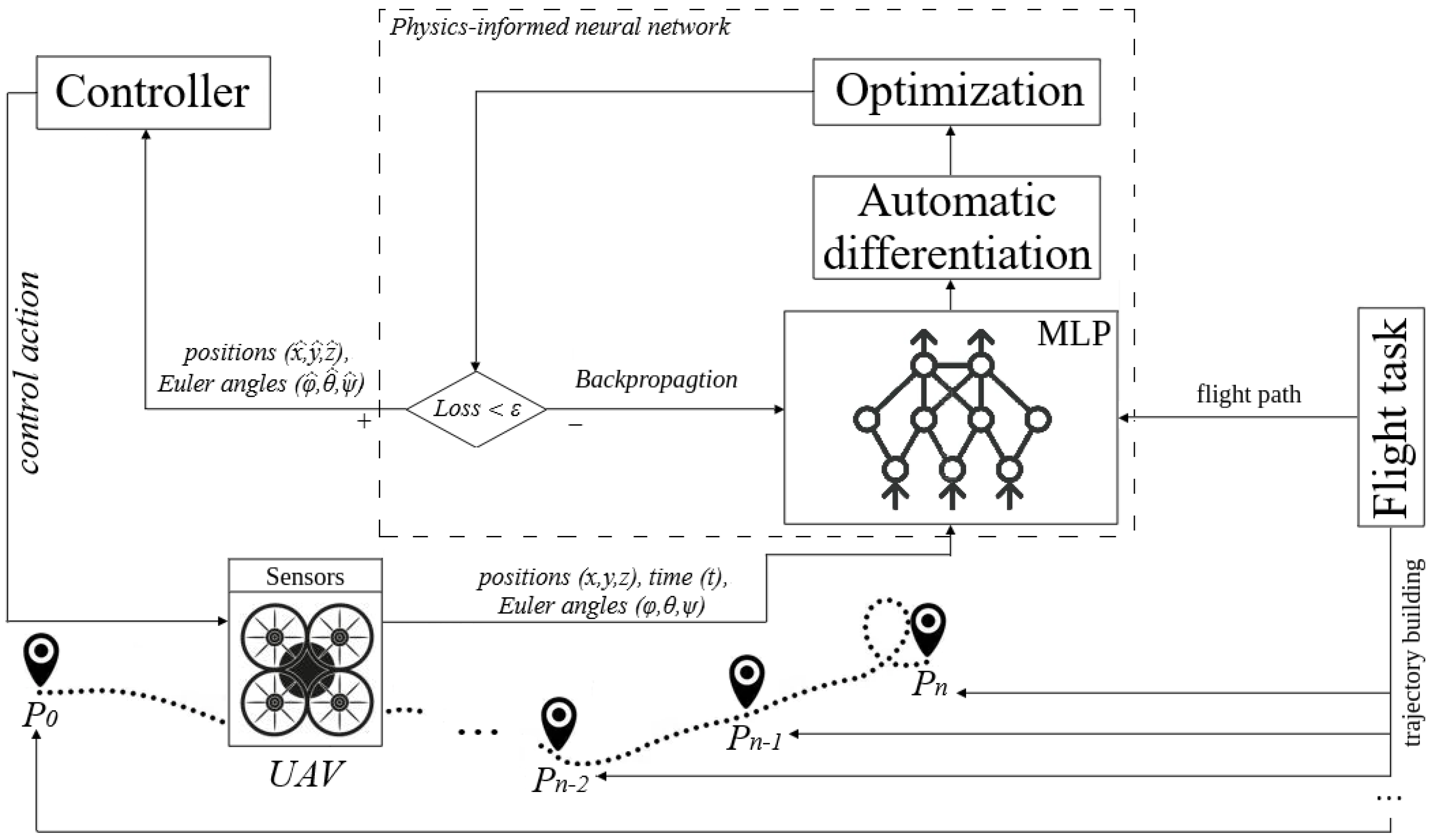
3. The Proposed Physics-Informed Neural Network for Quadcopter Dynamics Modeling

3.1. Fractional Optimization Algorithms

The main role of optimization algorithms in neural networks is an updating of weights to values that make the output results more accurate. The most dispersed optimizers for minimizing loss function are SGD and Adam. These SOTA approaches search the loss function minimum, considering the gradient directions and exponential moving averages. However, such optimizers do not guarantee convergence to the global minimum neighborhood. They do not solve the problem of exploding and vanishing gradients, which prevent any further learning. In [26], we proposed fractional gradient descent with Riemann–Liouville, Caputo, and Grunwald–Letnikov derivatives for minimizing loss functions. The fractional gradient structure is more adaptive than conventional SGD and Adam optimizers. The main reason for choosing right derivatives is the Taylor series expansion, which is inconsistent with left derivatives. Consider that $f:{\mathbb{R}}^d\to \mathbb{R}$ is a continuous function. The Riemann–Liouville right integral ${}_{a\hspace{0.17em}\hspace{0.17em}\hspace{0.17em}\hspace{0.17em}}{}^{RL}D_x^{\alpha }$, defined on $[a,b]$ for $a,b\in \mathbb{R}$, has the following form:

$${}_{a\hspace{0.17em}\hspace{0.17em}\hspace{0.17em}\hspace{0.17em}}{}^{RL}D_x^{\alpha }{f}_i\left(x\right)={\displaystyle \frac{1}{\Gamma (n-\alpha )}}{\displaystyle \frac{d^n}{d{x}^n}}{\int }_a^x{\displaystyle \frac{f_i\left(\tau \right)}{{(x-\tau )}^{\alpha +1-n}}}d\tau ,$$

(14)

where $\alpha >0$ is the order of the fractional derivatives, n is the order of the derivative of an integer degree, $f_i:\mathbb{R}\to \mathbb{R}$ is a continuous function, $i=1,\dots ,d$, and

$$\Gamma \left(\alpha \right)={\int }_0^{\infty }{\tau }^{\alpha -1}exp(-\tau )d\tau .$$

(15)

Expression (14) can be presented as follows:

$${}_{a\hspace{0.17em}\hspace{0.17em}\hspace{0.17em}\hspace{0.17em}}{}^{RL}D_x^{\alpha }{f}_i\left(x\right)=\sum _{j=0}^{\infty }{\displaystyle \frac{f_i^j\left(a\right)}{\Gamma (j+1-\alpha )}}{(x-a)}^{j-\alpha }.$$

(16)

It is necessary to mention that the Riemann–Liouville derivative of the constant is not equal to zero. Therefore, we omit the first item in (16). Next, we provide the Caputo fractional derivative, expressed as

$${}_a{}^{C}D_x^{\alpha }{f}_i\left(x\right)={\displaystyle \frac{1}{\Gamma (n-\alpha )}}{\int }_a^x{\displaystyle \frac{f_i^{\left(n\right)}\left(\tau \right)}{{(x-\tau )}^{\alpha +1-n}}}d\tau .$$

(17)

The corresponding Taylor expansion of (17) is

$${}_a{}^{C}D_x^{\alpha }{f}_i\left(x\right)=\sum _{j=n}^{\infty }{\displaystyle \frac{f_i^j\left(a\right)}{\Gamma (j+1-\alpha )}}{(x-a)}^{j-\alpha }.$$

(18)

In addition to the above fractional derivatives, there exists the Grunwald–Letnikov definition:

$${}_{a\hspace{0.17em}\hspace{0.17em}\hspace{0.17em}\hspace{0.17em}}{}^{GL}D_x^{\alpha }{f}_i\left(x\right)=\underset{h\to 0}{lim}{\displaystyle \frac{1}{h^{\alpha }}}\sum _{j=0}^{{\displaystyle \frac{x-a}{h}}}{\displaystyle \frac{{(-1)}^j\Gamma (\alpha +1)}{\Gamma (j+1)\Gamma (\alpha -j+1)}}{f}_i(x-jh).$$

(19)

$${}_{a\hspace{0.17em}\hspace{0.17em}\hspace{0.17em}\hspace{0.17em}}{}^{GL}D_x^{\alpha }{f}_i\left(x\right)=\sum _{j=0}^n{\displaystyle \frac{f_i^{\left(j\right)}\left(a\right)}{\Gamma (j+1-\alpha )}}{(x-a)}^{j-\alpha }+{\displaystyle \frac{1}{\Gamma (n-\alpha +2)}}{\int }_a^x{f}_i^{(n+1)}\left(\tau \right){(x-\tau )}^{n+1-\alpha }d\tau .$$

(20)

For addressing the constant derivation problem for GFDGD, we omit the first item in (20). The FGD has the following description:

$${\theta }_t={\theta }_{t-1}-{\displaystyle \frac{{\gamma }_t{}_0{}^T\nabla _{{\theta }_t}^{\alpha }f\left({\theta }_t\right)}{(\sqrt{{\widehat{v}}_t}+ϵ)\sqrt{(1+{\beta }_0^2)+{\beta }_0^2}}},$$

(21)

where ${}_0{}^T\nabla _{{\theta }_t}^{\alpha }f\left({\theta }_t\right)$ is the fractinal gradient.

For estimating the quality of optimization algorithms, there exist the convergence rate and stability analysis.

In [34], the authors considered a convergence-rate-estimation methodology. This resulted in a sufficient theoretical analysis of the optimization algorithms. The convergence rate metric, regret bound, is defined as follows:

$$\begin{array}{c}\hfill R\left(T\right):={\displaystyle \sum _{t=1}^T}[f\left({\theta }_t\right)-f\left({\theta }^{*}\right)],\end{array}$$

(22)

where $f\left({\theta }_t\right)$ is a continuous function and ${\theta }^{*}=argmi{n}_{\theta }{\sum }_{t=1}^{T}f\left({\theta }_t\right)$, where T is the number of iterations. The corresponding Lebesgue norms $L^2\left(\mathbb{R}\right)$ are defined as follows:

$$\begin{array}{c}\hfill \parallel g_t{\parallel }_2\le G,\end{array}$$

(23)

$$\begin{array}{c}\hfill \parallel {\theta }_n-{\theta }_m{\parallel }_2\le D,\end{array}$$

(24)

for $G,D>0$ and $m,n\in \{1,\dots ,T\}$. Suppose the loss function $f\left({\theta }_t\right)$ is convex. By using the property of the convex function, we provide that

$$\begin{array}{c}\hfill f\left(x\right)-f\left(y\right)\le \langle \nabla f\left(\theta \right(t\left)\right),x-y\rangle ,\end{array}$$

(25)

for all $x,y\in {\mathbb{R}}^d$. The regret bound estimation $R\left(T\right)$ determines the convergence rate of the optimization algorithm. The vast majority of SOTA Adam-type optimizers are $O\left(\sqrt{T}\right)$.

Theorem 1

([26]). If the objective function $f\left(\theta \left(t\right)\right):{\mathbb{R}}^d\to \mathbb{R}$ is continuous, ${\gamma }_t>0$ is the learning rate, $\alpha >0$, and conditions (9–11) hold, then the regret bound of the proposed FGD is

$$\begin{array}{c}\hfill R\left(T\right)\le {\displaystyle \frac{\Gamma (2-\alpha )D^2{\delta }^{\alpha -1}}{2{\gamma }_t}}+{\displaystyle \frac{G^2{(D+\delta )}^{1-\alpha }}{2\Gamma (2-\alpha ){\sum }_{t=1}^T{\gamma }_t}},\end{array}$$

(26)

for $\alpha \in (0,1]$, and

$$\begin{array}{c}\hfill R\left(T\right)\le {\displaystyle \frac{\Gamma (2-\alpha )D^2{(D+\delta )}^{\alpha -1}}{2{\gamma }_T}}+{\displaystyle \frac{G^2{\delta }^{1-\alpha }}{2\Gamma (2-\alpha ){\sum }_{t=1}^T{\gamma }_t}},\end{array}$$

(27)

for $\alpha >1$.

Next, we consider the stability analysis [35]. We consider the standard setting of supervised learning. Suppose that we are given n samples $S=(z_1,\dots ,z_n)$, each lying in some sample space $\mathcal{Z}$ and drawn i.i.d. according to a distribution $P\in \mathcal{P}$. The standard decision-theoretic approach is to estimate a parameter $\theta \in {\mathbb{R}}^d$ by minimizing a loss function of the form $l(\theta ;z)$, which measures the fit between the model indexed by the parameter $\theta \in {\mathbb{R}}^d$ and the sample $z\in \mathcal{Z}$.

Given the collection S of n samples and a loss function l, the principle of empirical risk minimization is based on the objective function

$$\begin{array}{c}\hfill R_S\left(\theta \right)={\displaystyle \frac{1}{n}}{\displaystyle \sum _{i=1}^n}l(\theta ;z).\end{array}$$

An algorithm outputs a model ${\widehat{\theta }}_S$-uniform stable if for all $k\in 1,\dots ,n$, for all data sample pairs $S=(z_1,\dots ,z_k,\dots ,z_n)$ and $S^{\prime }=(z_1,\dots ,z_k^{\prime },\dots ,z_n)$, each $z_i$ or $z_k^{\prime }$ is i.i.d sampled from P, and we have

$$\begin{array}{c}\hfill {\mathcal{E}}_{stab}(\widehat{\theta }\left(T\right),l,P,z)={\displaystyle \underset{z\in \mathcal{Z}}{sup}}|l({\widehat{\theta }}_S;z)-l({\widehat{\theta }}_{S^{\prime }};z)|.\end{array}$$

Theorem 2

([26]). Given a data distribution P, under the assumption that $l\left(\dot{,}z\right)$ is a convex, L-Lipschitz, and β-smooth function for every $z\in \mathcal{Z}$, the gradient method with constant step-size $\gamma \le {\displaystyle \frac{1}{\beta }}$ on the empirical risk $R_S$ with sample size n, which outputs $\widehat{\theta }\left(T\right)$ at iteration T, has the following uniform stability bound for all $T\ge 1$:

$$\begin{array}{c}\hfill {\mathcal{E}}_{stab}(\widehat{\theta }\left(T\right),l,P,n)\le {\displaystyle \frac{2\gamma L^{2}T}{n\Gamma (2-\alpha )}}.\end{array}$$

As one can see, the fractional optimization algorithms have convergence and stability estimations, which are proper for neural network training.

Considering the theorems above, one can conclude that optimization algorithms RLFGD, CFGD, and GLFGD have the $O\left(\sqrt{T}\right)$ convergence rate and $O\left(T\right)$ stability, which are admissible for modern neural network structures. Therefore, one can apply these optimizers in a PINN for UAV dynamics modeling.

3.2. The Proposed Physics-Aware Machine Learning Controller

Physics-aware machine learning in mathematical physics and control theory plays almost the same role as traditional numerical methods, such as the finite difference, element, volume, Runge–Kutta, and Adams approaches. One of the conventional models in physics-aware machine learning is a physics-informed neural network. Unlike the SOTA numerical methods, such a model is universal. It means that it can be applied to partial differential, integral, and functional equations. Most importantly, a PINN can solve the system of differential equations that construct the quadcopter dynamics model.

First, we focus on the general PINN model with FGD, solving a system of differential equations. We consider the input parameters, such as positions $x,y,z$, Euler angles $\varphi ,\theta ,\psi$, time t, and the flight task. Afterwards, we build the multilayer perceptron. The hidden layers are defined as follows:

$$\begin{array}{c}\hfill y^{\left(l\right)}=\omega \left(w^{(l-1)}\times {\left[y^{(l-1)}\right]}^T\right),\end{array}$$

(28)

where $y^l=[y_1^l,\dots ,y_{m_l}^l]$, $\omega$ is the activation function, $w^{l-1}$ is the weight matrix, and for $l=L$ the output parameters are $\widehat{x},\widehat{y},\widehat{z},\widehat{\varphi },\widehat{\theta },\widehat{\psi }$. Next, an automatic differentiation layer builds the system of equations:

$$\left\{\begin{array}{c}{\mathcal{N}}_1(t,x,y,z,\varphi ,\theta ,\psi ,\dot{x},\dots ,;{\lambda }_1)=0\hfill \\ \dots \hfill \\ {\mathcal{N}}_P(t,x,y,z,\varphi ,\theta ,\psi ,\dot{x},\dots ,;{\lambda }_P)=0\hfill \end{array}\right..$$

Afterwards, we define the functions:

$${\mathcal{F}}_i={\mathcal{N}}_i(t,x,y,z,\varphi ,\theta ,\psi ,\dot{x},\dots ,;{\lambda }_1),\mathrm{for}i=1,\dots ,P.$$

The function $Loss$ is determined as

$$Loss=\sum _{j=1}^{P}Los{s}_{{\mathcal{F}}_j}.$$

(29)

As the loss function, we consider the mean square error (MSE), the mean absolute error (MAE), and the integral squared error (ISE):

$$MS{E}_{{\mathcal{F}}_j}={\displaystyle \frac{1}{N_{{\mathcal{F}}_j}}}\sum _{i=1}^{N_{{\mathcal{F}}_j}}{\left({\mathcal{F}}_j\right)}^2,MA{E}_{{\mathcal{F}}_j}={\displaystyle \frac{1}{N_{{\mathcal{F}}_j}}}\sum _{i=1}^{N_{{\mathcal{F}}_j}}\left|{\mathcal{F}}_j\right|,IS{E}_{{\mathcal{F}}_j}={\displaystyle \frac{1}{N_{{\mathcal{F}}_j}}}{\int }_{s=0}^{S_{{\mathcal{F}}_j}}{\left({\mathcal{F}}_j\right)}^{2}ds.$$

The optimization algorithms RLFGD, CFGD, and GLFGD minimize these loss functions, and the backpropagation procedure updates the weights. This process repeats L times. The scheme of the physics-informed neural network is shown in Figure 2:

The more detailed work of the proposed physics-informed neural network with fractional gradient descent for quadcopter dynamics modeling is demonstrated in Algorithm 1.

In line 15 of Algorithm 1, ⊙ is the Hadamard multiplication, expressed as

$$\begin{array}{c}\hfill {(a_1,\dots ,a_n)}^T\odot {(b_1,\dots ,b_n)}^T={(a_1·b_1,\dots ,a_n·b_n)}^T\end{array}$$

for $a,b\in \mathbb{R}$. The backpropagation updates weights as

$$\begin{array}{c}\hfill w_k(i+1)=w_k\left(i\right)-\eta ({}_0{}^T\nabla _w^{\alpha }Loss\left(i\right)+\mu b(i+1))\end{array}$$

(30)

where $b(i+1)=\mu b\left(i\right)+(1-\tau )({}_0{}^T\nabla _w^{\alpha }Loss\left(i\right)+\lambda w_k\left(i\right))$ ($\tau$ is the damping parameter), $\gamma$ is the learning rate, $F_{Dir}$ is the Fisher matrix, and $w_k\in {\mathbb{R}}^n$ is a vector expressing weights. Next, we put the proposed PINN with FGD in the control system of the quadcopter in Figure 3.

The quadcopter flight is through the destination points $P_0,\dots ,P_n$, which is pairwise connected by the desired trajectory. The UAV sensors transmit its positions $x,y,z$, Euler angles $\varphi ,\theta ,\psi$, and time t. These input data and flight tasks are input parameters, which the MLP processes and gives to the automatic differentiation layer. This layer substitutes outputs in the quadcopter dynamics model. Next, one builds the loss function $Loss$. If the $Loss$ is greater than the required error $ϵ$, the fractional gradient descent finds the objective function minimum, and the backpropagation procedure updates the weights. If $Loss<ϵ$, then one transmits the final approximate solutions in the controller, which acts as a quadcopter.

Algorithm 1: Physics-informed neural network algorithm with fractional gradient descent for UAV dynamics modeling.

Input: $y_0=(x,y,z,\varphi ,\theta ,\psi )\in {\mathbb{R}}^6$ (input data), $d\in \mathbb{R}$ (desired output), $w\in {\mathbb{R}}^6\times {\mathbb{R}}^6$   (weights), $\sigma$ (activation function), $\lambda$ (weight decay), $\mu$ (momentum), $\tau$ (damping),   $T\in \{RL,C,GL\}$ (type of fractional derivative) Output: $\widehat{u}$ (approximate solution), $Loss\in \{MAE,MSE,ISE\}$ (loss function) 1:  for i from 1 to N do 2:     for l from 1 to L do 3:       $y^{(l+1)}\left(i\right)\leftarrow \sigma \left(w^{\left(l\right)}\left(i\right)y^{\left(l\right)}\left(i\right)\right)$ 4:     end for 5:     $\widehat{u}\left(i\right)\leftarrow \sigma \left(w^{\left(L\right)}\left(i\right)y^{\left(L\right)}\left(i\right)\right)$ 6:     for j from 1 to P do 7:       ${\mathcal{F}}_j\leftarrow {\mathcal{N}}_j(t,x,y,z,\varphi ,\theta ,\psi ,\dot{x},\dots ,;{\lambda }_j)$ 8:     end for 9:     $Loss\left(i\right)\leftarrow {\sum }_{j=1}^{P}Los{s}_{{\mathcal{F}}_j}\left(i\right)+Los{s}_{IC}\left(i\right)$ 10:    $e\left(i\right)\leftarrow d-\widehat{u}\left(i\right)$ 11:    for l from 0 to L do 12:      if l = L then 13:         ${\delta }^{\left(L\right)}\left(i\right)\leftarrow {}_0{}^{T}D_{v^{\left(L\right)}\left(i\right)}^{\alpha }Loss\left(i\right)$ 14:      else 15:         ${\delta }^{\left(l\right)}\left(i\right)\leftarrow w^{(l+1)}\left(i\right){\delta }^{(l+1)}\left(i\right)\odot {}_0{}^{T}D_{v^{\left(l\right)}\left(i\right)}^{\alpha }y\left(i\right)$ 16:      end if 17:      for k from 0 to n do 18:         if $i>1$ then 19:           $b(i+1)\leftarrow \mu b\left(i\right)+(1-\tau )({\delta }^{\left(l\right)}\left(i\right)y^{(l-1)}\left(i\right)+\lambda w_k\left(i\right))$ 20:         else 21:           $b(i+1)\leftarrow {\delta }^{\left(l\right)}\left(i\right)y^{(l-1)}(i+1)+\lambda w_k\left(i\right)$ 22:         end if 23:         $g^{\left(l\right)}(i+1)\leftarrow g^{\left(l\right)}\left(i\right)+\mu b(i+1)$ 24:         $w_k^{\left(l\right)}(i+1)\leftarrow w_k^{\left(l\right)}\left(i\right)-\eta g^{\left(l\right)}(i+1)$ 25:      end for 26:    end for 27: end for

4. Experiments on Quadcopter Flight Dynamics

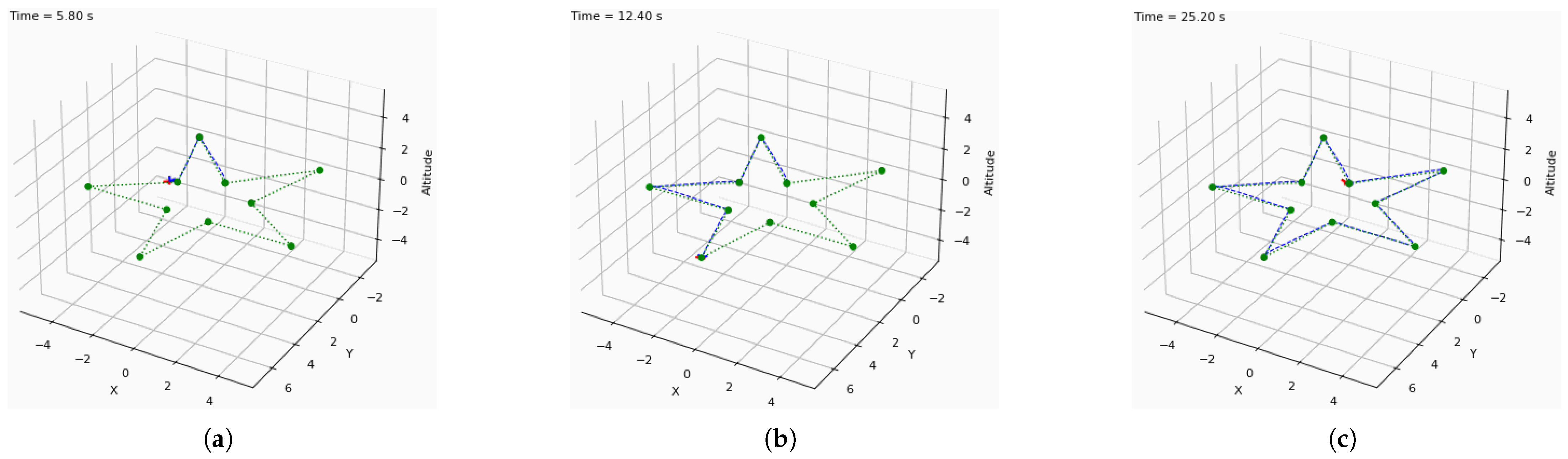
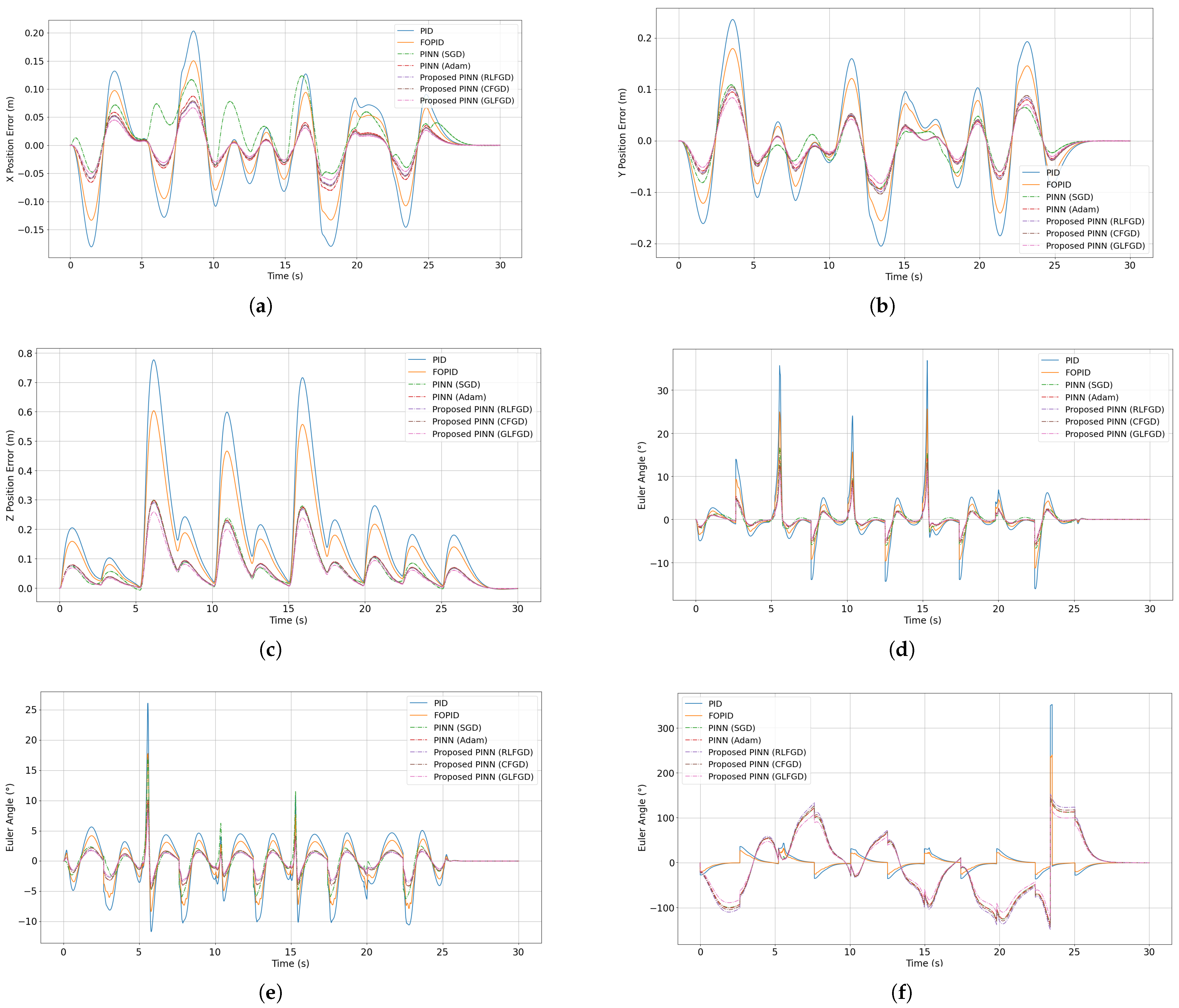
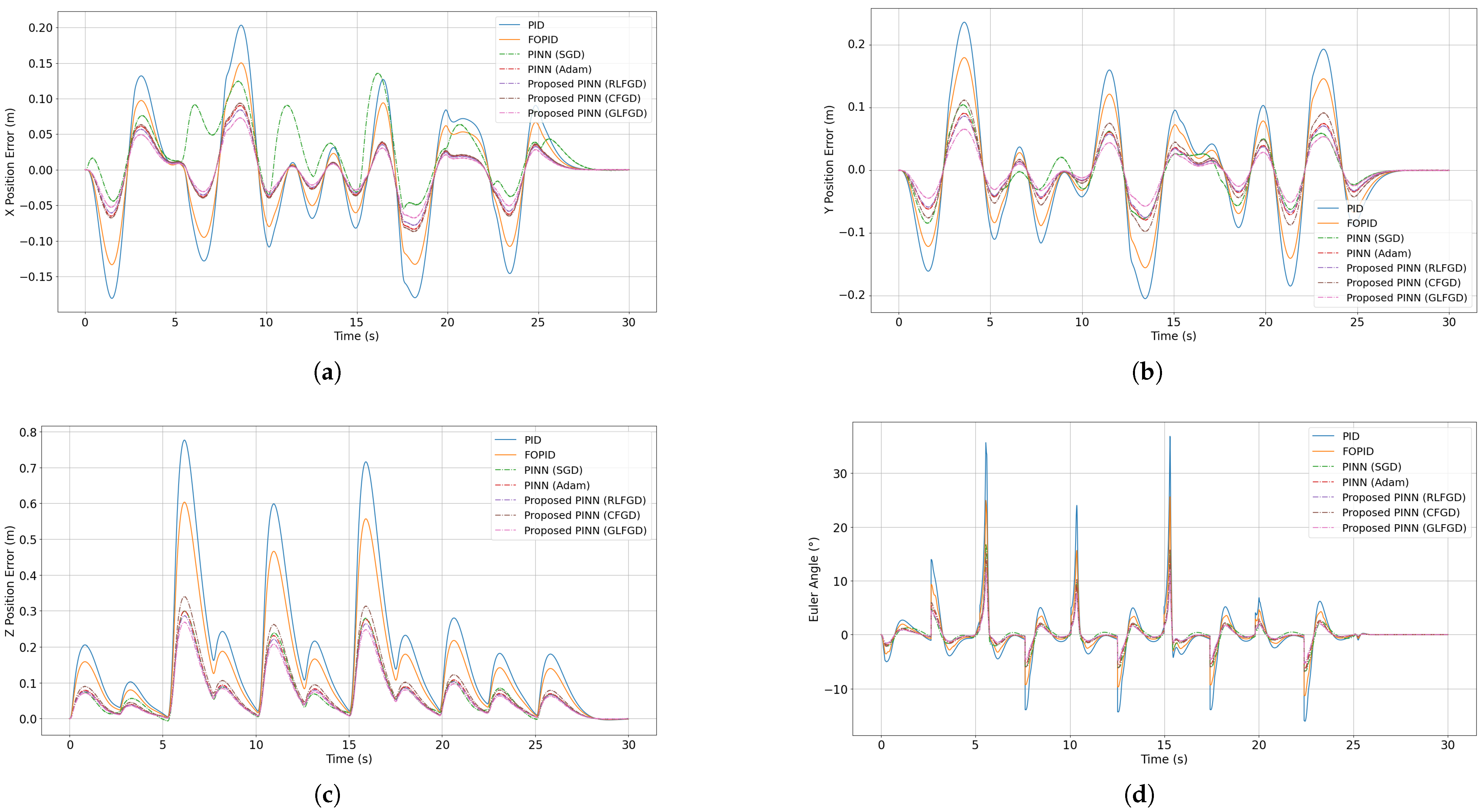
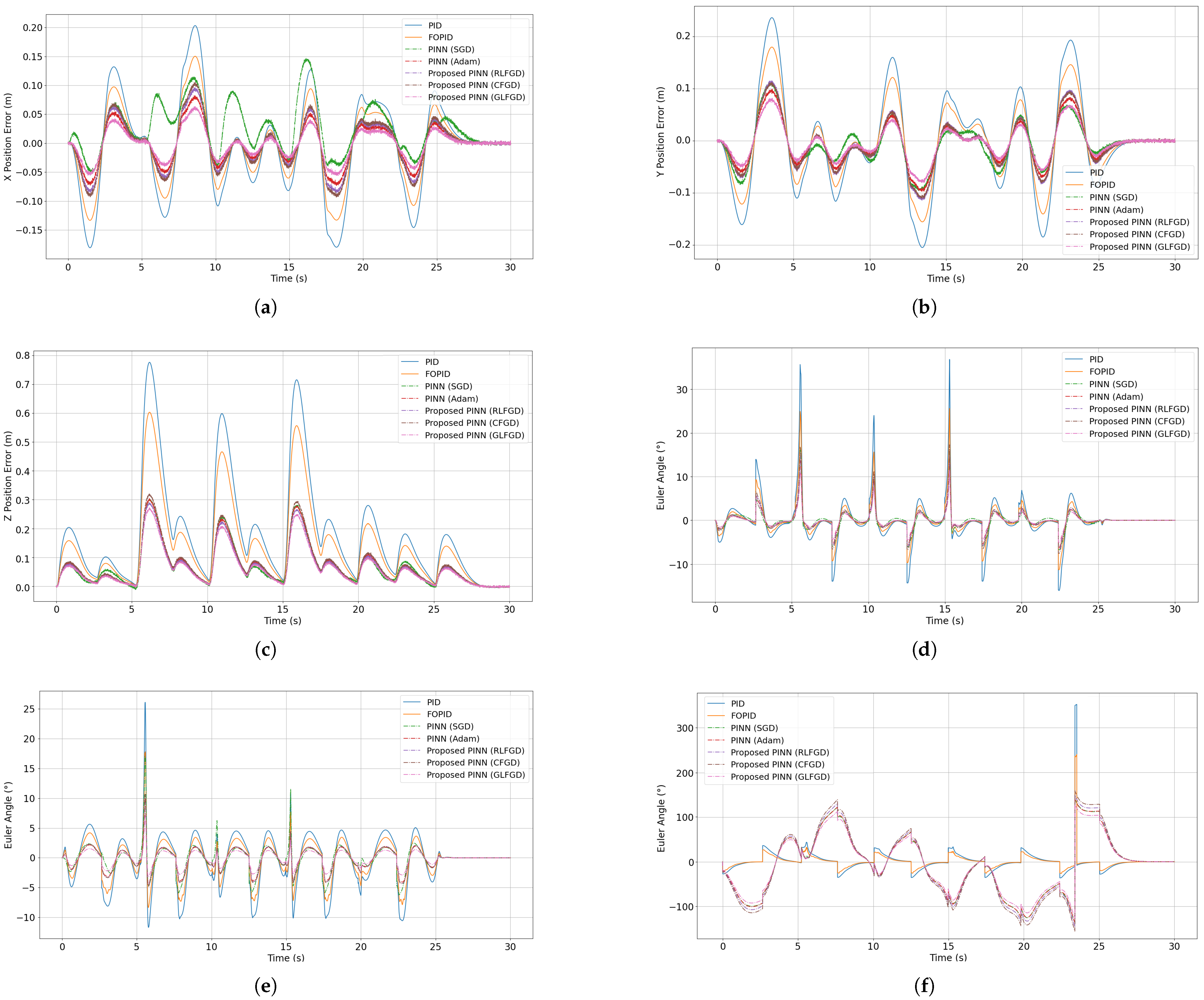
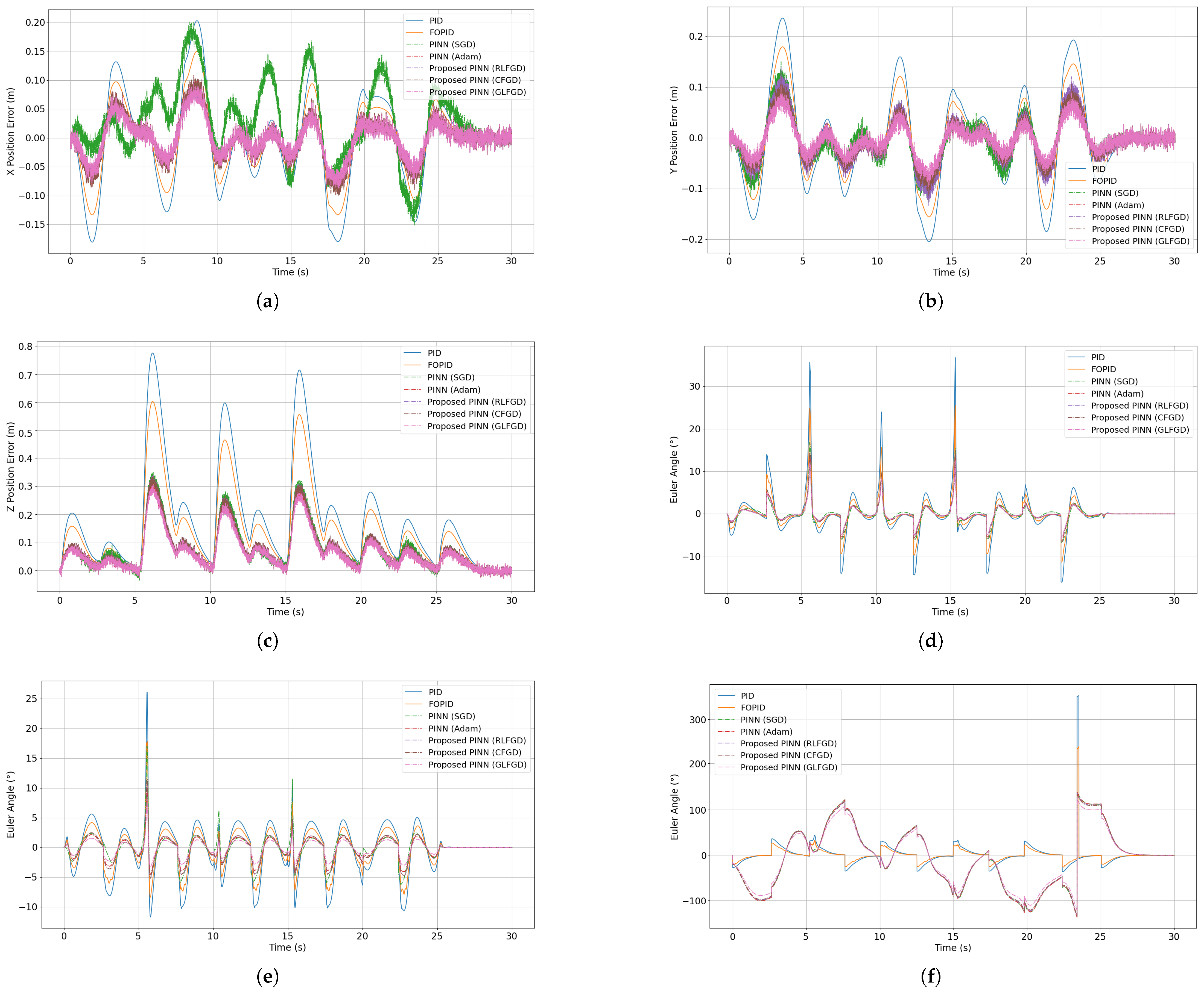
4.1. Results of the Proposed Physics-Informed Controller on Quadcopter Dynamics

In this section, we provide the results of UAV controllers based on a PID and the proposed fractional PINN scheme.

The proposed physics-informed neural networks were implemented via Python 3.10.2, using quadsim, pytorch, numpy, and matplotlib libraries. The training process was realized on Intel Core i7-8550U CPU, 1.80 GHz, Total Threads 8, Internal Memory 8 GiB. As the experiment, we considered the “star” flight trajectory, with the reference position and Euler angles parameters. Such a trajectory is shown in Figure 4:

The mass of the drone was $1.2$ kg, the arm length was $0.16$ m, the motor height was $0.05$ m, and the rotor moment inertia was $2.7\times {10}^{-5}$. For estimating the control quality given by the PID and the proposed PINN architectures, we used the mean absolute, mean square, and integral squared errors. In Figure 4, we demonstrate the positions, velocities, Euler angles, and angular velocities received by the best model among the SOTA and the proposed approaches. In this section, the proposed PINN with FGD contained the MLP with 6 hidden layers, 128 neuron layers, and $tanh$ activation function. For the FGD, the learning rate was $\eta =0.001$, $\alpha =1.5$, in fractional gradient $a=0$, weight decay $\lambda =0$, momentum $\mu =0.99$. The number of epochs was $10,000$. In Figure 5, we show the positional and angular errors achieved by the proposed and SOTA approaches.

Figure 6 demonstrates the errors of the SOTA and the proposed controllers. The proposed PINN with Grunwald–Letnikov attained the best results of the x- and y-axis errors, shown in Figure 6a–c. The second-most-accurate results were achieved by the PINN with the Caputo derivative. The PINN with Adam and RLFGD showed almost similar errors. The highest error values belonged to the PID and FOPID controllers. Considering the Euler angle errors in Figure 6d,e, the best result belonged to the PINN with GLFGD. The second-most-accurate results belonged to the PINN with CFGD. The PINN with Adam and RLFGD showed approximately the same error values. The SOTA PID and FOPID had the greatest error values, which can be seen in artifacts. In Figure 6f, the PID-based controllers show better results than the PINN-based analogs. However, the SOTA approaches had a high error value in the artifact moments. Such phenomena can be explained by the belonging of the PID and FOPID to linear systems. This flaw can be crucial in obstacle avoidance.

Considering the position graphs in Figure 5a–c, one can conclude that the PINN had better results then the best PID model attained. In Figure 5c, it can be seen that the PINN controller let the quadcopter hold the z-axis coordinate with less changes than the PID analogs. Reviewing the velocity Figure 5d–f, the proposed PINN controller at rapid stops showed results closer to those desired. In particular, this fact held for the z-axis, which is shown in Figure 5f. Analyzing the Euler angles in Figure 5g–i, the proposed physics-informed neural network with fractional derivatives attained values closer to those desired than the fractional PID. From Figure 5j–l, the angular velocities results of the PINN were closer to the the desired values at the artifact moments, where the PID could not handle the rapid loss and growth.

The proposed PINN with GLFGD gave the most accurate approximate trajectory $x,y,z$ with the following error values: MAE—$(3.205\times {10}^{-2},3.796\times {10}^{-2},2.411\times {10}^{-2})$, MSE—$(1.790\times {10}^{-3},1.842\times {10}^{-3},1.842\times {10}^{-3})$, and ISE—$(1.099,3.894,4.467)$. Meanwhile, the PINN with CFGD gave MAE—$(3.485\times {10}^{-2},4.003\times {10}^{-2},2.763\times {10}^{-2})$, MSE—$(2.041\times {10}^{-3},2.153\times {10}^{-3},1.384\times {10}^{-3})$, and ISE—$(4.048,4.782,0.229)$. The results in

Table 1. MAE, MSE, and ISE of quadcopter positions received by different proportional–integral–derivative and physics-informed models.

Model	MAE			MSE			ISE			Time, s
	$\mathit{x}\mathbf{\times }{\mathbf{10}}^{\mathbf{-}\mathbf{2}}$	$\mathit{y}\mathbf{\times }{\mathbf{10}}^{\mathbf{-}\mathbf{2}}$	$\mathit{z}\mathbf{\times }{\mathbf{10}}^{\mathbf{-}\mathbf{2}}$	$\mathit{x}\mathbf{\times }{\mathbf{10}}^{\mathbf{-}\mathbf{3}}$	$\mathit{y}\mathbf{\times }{\mathbf{10}}^{\mathbf{-}\mathbf{3}}$	$\mathit{z}\mathbf{\times }{\mathbf{10}}^{\mathbf{-}\mathbf{3}}$	$\mathit{x}\mathbf{\times }{\mathbf{10}}^{\mathbf{0}}$	$\mathit{y}\mathbf{\times }{\mathbf{10}}^{\mathbf{0}}$	$\mathit{z}\mathbf{\times }{\mathbf{10}}^{\mathbf{0}}$
PID	4.841	5.026	4.993	3.804	3.758	3.922	5.877	6.138	0.892	14.32
FOPID	4.573	4.704	4.429	3.545	3.179	2.834	5.192	5.336	0.691	15.88
PINN (SGD)	3.947	4.611	3.404	4.536	4.592	2.899	4.681	5.109	0.474	18.25
PINN (Adam)	3.690	4.252	2.983	2.508	2.459	1.643	4.189	4.919	0.263	19.04
Proposed PINN (RLFGD)	3.858	4.366	3.137	4.660	4.753	3.033	4.757	5.302	0.564	22.14
Proposed PINN (CFGD)	3.485	4.003	2.763	2.041	2.150	1.384	4.048	4.782	0.229	20.60
Proposed PINN (GLFGD)	3.205	3.796	2.411	1.790	1.842	1.099	3.894	4.467	0.192	21.89

and

Table 2. MAE, MSE, and ISE of quadcopter Euler angles received by different proportional–integral–derivative and physics-informed models.

Model	MAE			MSE			ISE			Time, s
	$\mathit{\varphi }\mathbf{\times }{\mathbf{10}}^{\mathbf{-}\mathbf{2}}$	$\mathit{\theta }\mathbf{\times }{\mathbf{10}}^{\mathbf{-}\mathbf{2}}$	$\mathit{\psi }\mathbf{\times }{\mathbf{10}}^{\mathbf{-}\mathbf{2}}$	$\mathit{\varphi }\mathbf{\times }{\mathbf{10}}^{\mathbf{-}\mathbf{2}}$	$\mathit{\theta }\mathbf{\times }{\mathbf{10}}^{\mathbf{-}\mathbf{2}}$	$\mathit{\psi }\mathbf{\times }{\mathbf{10}}^{\mathbf{-}\mathbf{2}}$	$\mathit{\varphi }\mathbf{\times }{\mathbf{10}}^{\mathbf{0}}$	$\mathit{\theta }\mathbf{\times }{\mathbf{10}}^{\mathbf{0}}$	$\mathit{\psi }\mathbf{\times }{\mathbf{10}}^{\mathbf{0}}$
PID	1.973	1.854	2.042	3.662	3.653	3.583	4.867	5.057	1.463	14.32
FOPID	1.774	1.662	1.950	3.114	2.948	3.434	4.492	4.804	1.297	15.88
PINN (SGD)	1.380	1.441	2.711	2.407	2.473	4.882	4.215	4.734	1.996	18.25
PINN (Adam)	1.354	1.399	2.376	1.942	2.030	4.493	4.189	4.704	1.944	19.04
Proposed PINN (RLFGD)	1.439	1.448	2.835	2.689	2.557	5.023	4.260	4.773	2.093	22.14
Proposed PINN (CFGD)	1.328	1.341	2.047	1.645	1.890	4.086	4.111	4.548	1.827	20.60
Proposed PINN (GLFGD)	1.288	1.305	2.049	1.268	1.643	3.918	4.033	4.286	1.636	21.89

show that the PINN with Adam worked more accurately than the PINN with RLFGD. Among the SOTA approaches, the least error values given were FOPID with the Caputo derivative. The highest error value was achieved by the conventional PID. In the case of Euler angle errors, the proposed techniques showed better results only for the $\varphi$ and $\theta$ parameters. However, the PID and FOPID achieved the least error values for $\psi$ compared to the PINN-based controllers. The PINN with GLFGD showed MAE—$(1.288\times {10}^{-2},1.305\times {10}^{-2},1.849\times {10}^{-2})$, MSE—$(1.268\times {10}^{-3},1.643\times {10}^{-3},3.918\times {10}^{-3})$, and ISE—$(4.033,4.286,1.636)$. The second-most-accurate results belonged to the PINN with CFGD: MAE—$(1.328\times {10}^{-2},1.341\times {10}^{-2},2.047\times {10}^{-2})$, MSE—$(1.645\times {10}^{-3},1.890\times {10}^{-3},4.086\times {10}^{-3})$, and ISE—($4.111,4.548,1.827)$. The PID and FOPID approaches simulated the drone flight with less time consumption than the proposed PINN with FGD. However, the proposed technique significantly reduced the error values of the position and attitude variables.

In the next subsection, we verify the work of the proposed physics-informed neural network with fractional gradient descent in cases of changing the activation function and hidden layers truncation.

4.2. Ablation Study

For the better understanding of the work of PINN-based controllers, we considered the ablations study. In other words, we determined which modules let the PINN achieve the best accuracy.

We considered the neural network architecture with fewer hidden layers and more simple activation functions. Firstly, we replaced the $tanh$ activation functions at the proposed PINN by sigmoid function $\sigma$. The MLP structure and parameters for the FGD remained the same. The errors of this model are demonstrated in Figure 7:

The differences between the graphs in Figure 6a–f and Figure 7a–f are not clear. The errors of positions and Euler angles visually are same. Therefore, we need to clarify the results using

Table 3. MAE, MSE, and ISE of quadcopter positions received by different proportional–integral–derivatives and a physics-informed neural network with $\sigma$ activation function and six hidden layers.

Model	MAE			MSE			ISE			Time, s
	$\mathit{x}\mathbf{\times }{\mathbf{10}}^{\mathbf{-}\mathbf{2}}$	$\mathit{y}\mathbf{\times }{\mathbf{10}}^{\mathbf{-}\mathbf{2}}$	$\mathit{z}\mathbf{\times }{\mathbf{10}}^{\mathbf{-}\mathbf{2}}$	$\mathit{x}\mathbf{\times }{\mathbf{10}}^{\mathbf{-}\mathbf{3}}$	$\mathit{y}\mathbf{\times }{\mathbf{10}}^{\mathbf{-}\mathbf{3}}$	$\mathit{z}\mathbf{\times }{\mathbf{10}}^{\mathbf{-}\mathbf{3}}$	$\mathit{x}\mathbf{\times }{\mathbf{10}}^{\mathbf{0}}$	$\mathit{y}\mathbf{\times }{\mathbf{10}}^{\mathbf{0}}$	$\mathit{z}\mathbf{\times }{\mathbf{10}}^{\mathbf{0}}$
PINN (SGD)	3.914	3.864	3.989	2.826	2.801	2.872	5.166	5.390	0.704	18.47
PINN (Adam)	3.862	3.982	4.011	2.704	2.680	2.923	5.111	5.462	0.644	18.94
Proposed PINN (RLFGD)	3.942	3.861	3.897	2.581	2.853	2.722	5.263	5.149	0.594	21.98
Proposed PINN (CFGD)	3.285	3.633	3.839	2.402	2.338	2.814	4.899	5.030	0.593	20.86
Proposed PINN (GLFGD)	3.091	3.302	3.466	2.185	2.120	2.449	4.848	4.835	0.603	22.05

and

Table 4. MAE, MSE, and ISE of quadcopter Euler angles received by different proportional–integral–derivatives and a physics-informed neural network with $\sigma$ activation function and six hidden layers.

Model	MAE			MSE			ISE			Time, s
	$\mathit{\varphi }\mathbf{\times }{\mathbf{10}}^{\mathbf{-}\mathbf{2}}$	$\mathit{\theta }\mathbf{\times }{\mathbf{10}}^{\mathbf{-}\mathbf{2}}$	$\mathit{\psi }\mathbf{\times }{\mathbf{10}}^{\mathbf{-}\mathbf{2}}$	$\mathit{\varphi }\mathbf{\times }{\mathbf{10}}^{\mathbf{-}\mathbf{2}}$	$\mathit{\theta }\mathbf{\times }{\mathbf{10}}^{\mathbf{-}\mathbf{2}}$	$\mathit{\psi }\mathbf{\times }{\mathbf{10}}^{\mathbf{-}\mathbf{2}}$	$\mathit{\varphi }\mathbf{\times }{\mathbf{10}}^{\mathbf{0}}$	$\mathit{\theta }\mathbf{\times }{\mathbf{10}}^{\mathbf{0}}$	$\mathit{\psi }\mathbf{\times }{\mathbf{10}}^{\mathbf{0}}$
PINN (SGD)	1.894	1.865	2.030	2.594	2.637	5.112	5.294	5.774	2.870	18.47
PINN (Adam)	1.757	1.745	1.930	2.654	2.576	4.943	5.202	5.628	2.744	18.94
Proposed PINN (RLFGD)	1.985	2.103	2.005	2.954	3.011	3.196	4.260	4.773	2.093	21.98
Proposed PINN (CFGD)	1.864	1.937	1.947	2.709	2.894	3.014	4.185	4.534	1.983	20.86
Proposed PINN (GLFGD)	1.880	1.805	1.949	2.768	2.643	2.918	4.033	4.286	1.636	22.05

:

Considering the results in Table 3 and Table 4, the difference between the PINN with $tanh$ and with $\sigma$ activation functions is obvious. The PINN with GLFGD gave the most accurate approximate trajectory $x,y,z$ with the following error values: MAE—$(3.091\times {10}^{-2},3.302\times {10}^{-2},3.466\times {10}^{-2})$, MSE—$(2.185\times {10}^{-3},2.120\times {10}^{-3},2.449\times {10}^{-3})$, and ISE—$4.848,4.539,0.603)$. The results given by the PINN with CFGD had the following errors: MAE—$(3.285\times {10}^{-2},3.633\times {10}^{-2},3.839\times {10}^{-2})$, MSE—$(2.402\times {10}^{-3},2.338\times {10}^{-3},2.814\times {10}^{-3})$, and ISE—$4.899,5.539,0.593)$. The results of the PINN with Adam were thirdmost in average accuracy among the other DD models. The worst results among the PINN models were achieved by RLFGD.

In Table 4, the best average result was the PINN with GLFGD with the following losses: MAE—$(1.880\times {10}^{-2},1.805\times {10}^{-2},1.949\times {10}^{-2})$, MSE—$(2.768\times {10}^{-3},2.643\times {10}^{-3},2.918\times {10}^{-3})$, and ISE—$4.033,4.286,1.636)$. Next, the second-most-accurate results were achieved via the PINN with CFGD. Among the DD models, the PINN with Adam and the PINN with RLFGD had the third- and the fourth-best results, in terms of the quality of quadcopter dynamics modeling.

Next, we consider a PINN with five hidden layers and the same activation function and FGD parameters. The errors of this model are demonstrated in Figure 8:

In Figure 8, the quality of the solution attained by the proposed PINN with FGD was worse, as one can see in graphs (a)–(c). This fact can be explained by the trajectory shown in Figure 4. In this case, the angular parameters did not change much more than than the positional. The exact decrease in the results of the proposed truncated PINN with FGD is shown in

Table 5. MAE, MSE, and ISE of quadcopter positions received by different proportional–integral–derivatives and a physics-informed neural network with $\sigma$ activation function and five hidden layers.

Model	MAE			MSE			ISE			Time, s
	$\mathit{x}\mathbf{\times }{\mathbf{10}}^{\mathbf{-}\mathbf{2}}$	$\mathit{y}\mathbf{\times }{\mathbf{10}}^{\mathbf{-}\mathbf{2}}$	$\mathit{z}\mathbf{\times }{\mathbf{10}}^{\mathbf{-}\mathbf{2}}$	$\mathit{x}\mathbf{\times }{\mathbf{10}}^{\mathbf{-}\mathbf{3}}$	$\mathit{y}\mathbf{\times }{\mathbf{10}}^{\mathbf{-}\mathbf{3}}$	$\mathit{z}\mathbf{\times }{\mathbf{10}}^{\mathbf{-}\mathbf{3}}$	$\mathit{x}\mathbf{\times }{\mathbf{10}}^{\mathbf{0}}$	$\mathit{y}\mathbf{\times }{\mathbf{10}}^{\mathbf{0}}$	$\mathit{z}\mathbf{\times }{\mathbf{10}}^{\mathbf{0}}$
PINN (SGD)	4.943	4.992	4.615	3.904	3.876	3.710	6.062	5.398	0.806	15.74
PINN (Adam)	4.736	4.822	4.443	3.632	3.702	3.540	5.922	5.214	0.694	16.29
Proposed PINN (RLFGD)	4.839	4.784	4.510	3.806	3.689	3.693	5.453	5.837	0.713	19.34
Proposed PINN (CFGD)	4.316	4.606	4.485	3.723	3.575	3.800	5.225	5.529	0.685	18.83
Proposed PINN (GLFGD)	4.262	4.498	4.421	3.620	3.288	3.562	5.274	5.459	0.686	19.07

and

Table 6. MAE, MSE, and ISE of quadcopter Euler angles received by different proportional–integral–derivatives and a physics-informed neural networks with $\sigma$ activation function and five hidden layers.

Model	MAE			MSE			ISE			Time, s
	$\mathit{\varphi }\mathbf{\times }{\mathbf{10}}^{\mathbf{-}\mathbf{2}}$	$\mathit{\theta }\mathbf{\times }{\mathbf{10}}^{\mathbf{-}\mathbf{2}}$	$\mathit{\psi }\mathbf{\times }{\mathbf{10}}^{\mathbf{-}\mathbf{2}}$	$\mathit{\varphi }\mathbf{\times }{\mathbf{10}}^{\mathbf{-}\mathbf{2}}$	$\mathit{\theta }\mathbf{\times }{\mathbf{10}}^{\mathbf{-}\mathbf{2}}$	$\mathit{\psi }\mathbf{\times }{\mathbf{10}}^{\mathbf{-}\mathbf{2}}$	$\mathit{\varphi }\mathbf{\times }{\mathbf{10}}^{\mathbf{0}}$	$\mathit{\theta }\mathbf{\times }{\mathbf{10}}^{\mathbf{0}}$	$\mathit{\psi }\mathbf{\times }{\mathbf{10}}^{\mathbf{0}}$
PINN (SGD)	1.793	1.814	1.892	2.375	2.405	2.438	4.866	5.174	2.864	15.74
PINN (Adam)	1.565	1.595	1.699	2.103	2.284	2.273	4.637	4.940	2.545	16.29
Proposed PINN (RLFGD)	1.604	1.603	1.675	2.212	2.305	2.226	4.760	4.773	2.651	19.34
Proposed PINN (CFGD)	1.546	1.498	1.509	2.109	2.138	2.189	4.685	4.534	2.483	18.83
Proposed PINN (GLFGD)	1.527	1.464	1.534	2.072	2.173	2.114	4.584	4.492	2.336	19.07

:

According to the results in Table 5 and Table 6, one can see that the proposed PINN with $\sigma$ activation function and five hidden layers showed worse results. The PINN with GLFGD gave the most accurate approximate trajectory $x,y,z$ with the following error values: MAE—$(4.262\times {10}^{-2},4.498\times {10}^{-2},4.421\times {10}^{-2})$, MSE—$(3.620\times {10}^{-3},3.288\times {10}^{-3},3.562\times {10}^{-3})$, and ISE—($5.274,5.459,0.686)$. The results given by the PINN with CFGD had the following errors: MAE—$(4.316\times {10}^{-2},4.606\times {10}^{-2},4.485\times {10}^{-2})$, MSE—$(3.723\times {10}^{-3},3.575\times {10}^{-3},3.800\times {10}^{-3})$, and ISE—($5.225,5.539,0.685)$. The results of the PINN with Adam were the third in average accuracy among the other DD models. The worst results among the PINN models were achieved by RLFGD. In Table 4, the best average result was the PINN with GLFGD, with the following losses: MAE—$(1.527\times {10}^{-2},1.464\times {10}^{-2},1.509\times {10}^{-2})$, MSE—$(2.072\times {10}^{-3},2.173\times {10}^{-3},2.114\times {10}^{-3})$, and ISE—($4.584,4.492,2.336)$. The second-most-accurate result achieved was by the PINN with CFGD, with the following values: MAE—$(1.546\times {10}^{-2},1.498\times {10}^{-2},1.509\times {10}^{-2})$, MSE—$(2.109\times {10}^{-3},2.138\times {10}^{-3},2.189\times {10}^{-3})$, and ISE—($4.685,4.534,2.483)$.

Next, we verified training on a PINN with $\sigma$ activation function and four hidden layers.

In Figure 9, the quality of the solution did not suffice for the quality of the proposed model in Section 4.1, as one can see in graphs (a)–(c). This fact can be explained by the trajectory shown in Figure 4. In this case, the angular parameters did not change much more than the positional. The exact decrease in the results of the proposed truncated PINN with FGD is shown in

Table 7. MAE, MSE, and ISE of quadcopter positions received by different proportional–integral–derivatives and a physics-informed neural network with $\sigma$ activation function and four hidden layers.

Model	MAE			MSE			ISE			Time, s
	$\mathit{x}\mathbf{\times }{\mathbf{10}}^{\mathbf{-}\mathbf{2}}$	$\mathit{y}\mathbf{\times }{\mathbf{10}}^{\mathbf{-}\mathbf{2}}$	$\mathit{z}\mathbf{\times }{\mathbf{10}}^{\mathbf{-}\mathbf{2}}$	$\mathit{x}\mathbf{\times }{\mathbf{10}}^{\mathbf{-}\mathbf{3}}$	$\mathit{y}\mathbf{\times }{\mathbf{10}}^{\mathbf{-}\mathbf{3}}$	$\mathit{z}\mathbf{\times }{\mathbf{10}}^{\mathbf{-}\mathbf{3}}$	$\mathit{x}\mathbf{\times }{\mathbf{10}}^{\mathbf{0}}$	$\mathit{y}\mathbf{\times }{\mathbf{10}}^{\mathbf{0}}$	$\mathit{z}\mathbf{\times }{\mathbf{10}}^{\mathbf{0}}$
PINN (SGD)	5.946	5.893	5.684	4.042	3.935	4.147	6.236	6.272	1.101	13.46
PINN (Adam)	5.662	5.482	5.311	3.704	3.680	3.923	5.863	5.980	0.821	13.80
Proposed PINN (RLFGD)	5.539	5.013	4.802	3.881	3.799	3.994	5.894	5.849	0.836	14.72
Proposed PINN (CFGD)	5.276	5.608	5.548	3.463	3.498	3.814	5.682	5.530	0.704	14.19
Proposed PINN (GLFGD)	5.681	5.302	5.466	3.385	3.520	3.449	5.529	5.539	0.683	14.89

and

Table 8. MAE, MSE, and ISE of quadcopter Euler angles received by different proportional–integral–derivatives and a physics-informed neural networks with $\sigma$ activation function and four hidden layers.

Model	MAE			MSE			ISE			Time, s
	$\mathit{\varphi }\mathbf{\times }{\mathbf{10}}^{\mathbf{-}\mathbf{2}}$	$\mathit{\theta }\mathbf{\times }{\mathbf{10}}^{\mathbf{-}\mathbf{2}}$	$\mathit{\psi }\mathbf{\times }{\mathbf{10}}^{\mathbf{-}\mathbf{2}}$	$\mathit{\varphi }\mathbf{\times }{\mathbf{10}}^{\mathbf{-}\mathbf{2}}$	$\mathit{\theta }\mathbf{\times }{\mathbf{10}}^{\mathbf{-}\mathbf{2}}$	$\mathit{\psi }\mathbf{\times }{\mathbf{10}}^{\mathbf{-}\mathbf{2}}$	$\mathit{\varphi }\mathbf{\times }{\mathbf{10}}^{\mathbf{0}}$	$\mathit{\theta }\mathbf{\times }{\mathbf{10}}^{\mathbf{0}}$	$\mathit{\psi }\mathbf{\times }{\mathbf{10}}^{\mathbf{0}}$
PINN (SGD)	1.725	1.843	1.797	2.357	2.542	2.512	4.483	4.620	2.347	13.46
PINN (Adam)	1.968	1.997	1.964	2.583	2.744	2.803	4.602	4.726	2.595	13.80
Proposed PINN (RLFGD)	1.823	1.941	1.805	2.554	2.413	2.583	4.594	4.803	1.943	14.72
Proposed PINN (CFGD)	1.628	1.694	1.707	2.239	2.339	2.376	4.375	4.510	1.849	14.19
Proposed PINN (GLFGD)	1.618	1.643	1.639	2.220	2.386	2.324	4.203	4.357	1.522	14.89

.

In the results in Table 7 and Table 8, the difference between the PINN with $tanh$ and $\sigma$ activation functions is obvious. The PINN with GLFGD gave the most accurate approximate trajectory $x,y,z$ with the following error values: MAE—$(5.681\times {10}^{-2},5.302\times {10}^{-2},5.466\times {10}^{-2})$, MSE—$(3.385\times {10}^{-3},3.520\times {10}^{-3},3.449\times {10}^{-3})$, and ISE—($5.529,5.539,0.683)$. The results given by the PINN with CFGD had the following errors: MAE—$(5.276\times {10}^{-2},5.608\times {10}^{-2},5.548\times {10}^{-2})$, MSE—$(3.463\times {10}^{-3},3.498\times {10}^{-3},3.814\times {10}^{-3})$, and ISE—($5.682,5.530,0.704)$. The results for the PINN with RLFGD were the third in average accuracy among the other DD models. The worst results among the PINN models were achieved by Adam. In Table 4, the best average result was the PINN with GLFGD, with the following losses: MAE—$(1.618\times {10}^{-2},1.643\times {10}^{-2},1.639\times {10}^{-2})$, MSE—$(2.220\times {10}^{-3},2.386\times {10}^{-3},2.324\times {10}^{-3})$, and ISE—($4.203,4.357,1.522)$. The next-best average accuracy results were achieved by the PINN with CFGD. Among the DD models, the PINN with Adam and the PINN with RLFGD had the third- and the fourth-best results for the quality of quadcopter dynamics modeling.

Considering the results in Table 3, Table 4, Table 5, Table 6, Table 7 and Table 8, one can see that changing the tanh activation function by $\sigma$ and reducing the number of hidden layers decreased the quality of the quadcopter dynamics modeling. There was a significant decrease in the accuracy of parameters $x,y,z$, which can be seen in Figure 7 and Figure 8. The output parameters $\varphi ,\theta ,\psi$ had the least loss in accuracy. This can be explained by the trajectory (Figure 4), which is parallel to the $xOy$ plane. The changes in the Euler angles $\varphi ,\theta ,\psi$ were less noticeable than in positions $x,y,z$.

4.3. Steady State Performance

The drone’s steady state met at the beginning and end of the flight, as shown by the position and attitude errors. In the initial state $0\le t\le 2$, the hovering drone started the flight. The FOPID approach corrected the UAV positions and Euler angles with high errors, which is shown in Figure 6, Figure 7, Figure 8 and Figure 9. Meanwhile, the proposed PINN with FGD reduced the positional and angular errors at the start moment. For $5\le t\le 10$, the drone hovered for 1 second and then continued its movement. The position and attitude errors of the PID and FOPID significantly increased. The same increase occurred in the following time intervals: $[10.5,12]$, $[15.6,17.3]$, and $[20.1,22.5]$. The proposed PINN with FGD reduced the position errors by almost 2 times. In the case of attitude analysis, the $\varphi$ angle error of the PID and FOPID attained the maximal values for $t=5.3$ and $t=15.2$. The proposed PINN with FGD and conventional optimizers demonstrated an error of 2.5 times less than the PID and FOPID. Considering the $\theta$ angle, the FOPID and PID attained the maximal error value in $t=5.3$, while the proposed PINN with FGD reduced this error by almost 2 times. Considering the $\psi$ parameter, the PID and FOPID reached the highest error values at $t=23.9$. However, the average error of the MBC models was less than the proposed data-driven models.

The proposed physics-aware machine learning models control drone flight dynamics significantly better than model-based controllers. The main problem of PIDs and FOPIDs lies in integral and derivative blocks, which cannot handle non-smooth data domains. Moreover, they are designed as linear models. The proposed PINN with FGD experiences less impact from data non-smoothness because of the adaptive learning process. Therefore, the risk of rapid error growth in a PINN is less than in a PID.

5. Discussion

The PINN approach in the predictive control of UAV flight dynamics showed more accurate results compared to the SOTA PID techniques. It allowed us to build a trajectory with more accurate spatial coordinates, velocity, Euler angles, and angular velocities. In addition to the PIML approach, there exists a lot of research on UAV dynamics modeling with other types of reinforcement learning: LQR, LGM, PPO, and SAC. Moreover, the recent modification of the PID controller significantly improved the quality of trajectory building for UAV systems. In

Table 9. Evolution of methods for solving quadcopter dynamics problem.

Method	Year	Key Idea
PID [6]	2009	Summation of proportional, integral, and derivative of error.
Adaptive PID [36]	2013	Adaptive gains and robustifying adaptive terms.
Fractional PID [37]	2015	Fractional-order integral and derivative of error.
LQG [8]	2019	Linearization of the nonlinear control model.
LQR [9]	2020	Optimal control, where a quadratic cost function is minimized.
PINN [38]	2024	Self-learning approach with automatic differentiation.
Proposed PINN with FGD	2024	Fractional optimization of loss function.

, we present a brief overview of the evolution of controllers for UAV dynamic modeling.

The use of fractional gradient descent with Riemann–Liouville, Caputo, and Grunwald–Letnikov derivatives can handle the loss function minimization problem. However, this system has disadvantages. A PINN constructed on MLP cannot improve approximation with an increase in layer numbers. The main limitation of fractional gradient descent is the inability to solve the problem of exploding and vanishing gradients, which meet in non-smooth or plane domains of loss functions. Such a flaw deteriorates the learning process for arbitrary neural networks, because the optimizer cannot converge to the global minimum neighborhood of the objective function. Fractional-order and conventional first-order optimizers do not avoid local extreme points. To solve these problems, we plan to develop hybrid optimization algorithms, which consider the properties of gradient-based and population-based approaches. Modern physics-informed neural networks are based on multilayer perceptrons, which are already outdated. In our further research, we plan to build physics-aware machine learning models, considering the Kolmogorov–Arnold networks. Such networks are based on fundamental approximation theorems, which make them more adaptive under numerical problems. We provided the practical (steady state) performance in Section 4.3. We plan to provide robustness analysis in our further research. Therefore, the DD models for our UAV dynamics modeling will have to be improved complexly. As the next possible improvement, we will consider modified, local-operator, and non-singular kernel fractional derivatives. One of the most promising ways to improve loss function minimization is the utilization of Tarasov’s fractional derivatives. This scientist developed the fractional models in theoretical physics and mathematical economics. For the acceleration of loss function minimization, one can use scheduling, which can perform the convergence from $O\left(\sqrt{T}\right)$ to $O(logT)$. One of the most promising modifications is the minimization of loss function by hybrid optimization algorithms, which combine gradient, population, evolution, and other metaheuristic optimizers. Excellent examples of such optimizers are AdaSwarm [39], ADACO [40], and genetic PSO [41]. These approaches complement the error backpropagation methods and improve not only physics-informed neural networks but many other architectures. The application of fractional calculus in information geometry can give us new methods for data curation, executed by Kulback–Leibler, Jenssen divergences, and Wasserstein, Lévy–Prokhorov metrics. For example, natural and mirror descents are examples of information-geometric optimization algorithms, which analyze the loss function by the Fisher information matrix and Bergmann metrics, respectively. Currently, there is no fractional analog of the Fisher information matrix, regardless of the extension of Riemannian geometry via fractional calculus. The solving of this problem could involve the newest modification of information-geometric optimizers, like NGD, KFAC, E-KFAC, and AdaFisher. Moreover, information geometry allows for creating loss functions, which will analyze the correctness of outputs more accurately and completely. The inclusion of fuzzy layers allows us to analyze the solution of the system (1)–(3), reducing unnecessary computations. The utilization of DeepONets with self-attention layers can significantly raise UAV model tuning quality. The tensor decomposition of the input spatial and angular data by the CP [42], Tucker [43], and Tensor-Train [44] methods can accelerate learning, preserving the quality of the final trajectory. Moreover, replacing the multilayer perceptron block with the Kolmogorov–Arnold network [45] allows us not just to improve the quality of trajectory construction but also creates a new reinforcement learning direction in UAV systems modeling. $H_{\infty }$ filtering [46] can enhance the performance of quadcopter dynamics modeling. All these ideas can be helpful in modeling any type of UAV, such as tricopters, quadcopters, hexacopters, octocopters, and so on. If the UAV executes the command and reaches checkpoints faster then one can raise the quality of service of power lines [28], logistics [3], agriculture [29], and remote sensing [30].

6. Conclusions

The proposed PINN controller for UAV dynamics modeling showed better results than existing PID techniques. Moreover, the proposed model had less error value in spatial coordinates and Euler angles by 25–35% and 30–44%, respectively. In further research, in addition to the usual PINN architecture, we plan to use operator learning approaches, such as DeepONet and FNO, which analyze input variables and solutions. Fractional calculus has had a great influence on modern machine learning and control theory. The optimizers provided above are fractional analogs of first- and second-order gradient-based approaches. As one can see, the fractional control models significantly raised the model tuning quality, which motivated us to include all the ideas provided above for further modifications. In further research, we plan to apply the modified DD physics-aware machine-learning models in modeling the flight dynamics of the following UAVs: tricopters, hexacopters, and octacopters.

References

1. Su, J.; Zhu, X.; Li, S.; Chen, W.H. AI meets UAVs: A survey on AI empowered UAV perception systems for precision agriculture. Neurocomputing 2023, 518, 242–270. [Google Scholar] [CrossRef]
2. Lee, H.-W. Research on multi-functional logistics intelligent Unmanned Aerial Vehicle. Eng. Appl. Artif. Intell. 2022, 116, 105341. [Google Scholar] [CrossRef]
3. Dudukcu, H.V.; Taskiran, M.; Kahraman, N. UAV sensor data applications with deep neural networks: A comprehensive survey. Eng. Appl. Artif. Intell. 2023, 123, 106476. [Google Scholar] [CrossRef]
4. Ai, D.; Jiang, G.; Lam, S.K.; He, P.; Li, C. Computer vision framework for crack detection of civil infrastructure—A review. Eng. Appl. Artif. Intell. 2023, 117, 105478. [Google Scholar] [CrossRef]
5. Somanagoudar, A.G.; Mérida, W. Weather-aware energy management for unmannedaerial vehicles: A machine learning application with global data integration. Eng. Appl. Artif. Intell. 2025, 139, 109596. [Google Scholar] [CrossRef]
6. Yongjun, D.; Jianhong, W.; Jinlong, Z.; Xi, L. Design of quadcopter attitude controller based on data-driven model-free adaptive sliding mode control. Int. J. Dynam. Control 2024, 12, 1404–1414. [Google Scholar] [CrossRef]
7. Sahrir, N.H.; Basri, M.A.M. PSO–PID Controller for Quadcopter UAV: Index Performance Comparison. Arab. J. Sci. Eng. 2023, 48, 15241–15255. [Google Scholar] [CrossRef]
8. Lopez-Sanchez, I.; Moreno-Valenzuela, J. PID control of quadrotor UAVs: A survey. Annu. Rev. Control 2023, 56, 100900. [Google Scholar] [CrossRef]
9. Ihnak, M.S.A.; Edardar, M.M. Comparing LQR and PID Controllers for Quadcopter Control Effectiveness and Cost Analysis. In Proceedings of the IEEE 11th International Conference on Systems and Control (ICSC), Sousse, Tunisia, 18–20 December 2023. [Google Scholar]
10. Mardlijah; Alifah, Z.N. Control Design of Quadcopter using Linear Quadratic Gaussian (LQG). In Proceedings of the International Conference on Computer Engineering, Network, and Intelligent Multimedia (CENIM), Surabaya, Indonesia, 22–23 November 2022. [Google Scholar]
11. Berberich, J.; Köhler, J.; Müller, M.A.; Allgöwer, F. Data-Driven Model Predictive Control With Stability and Robustness Guarantees. IEEE Trans. Autom. Control 2021, 66, 1702–1717. [Google Scholar] [CrossRef]
12. Madani, T.; Benallegue, A. Backstepping Control for a Quadrotor Helicopter. In Proceedings of the 2006 IEEE/RSJ International Conference on Intelligent Robots and Systems, Beijing, China, 9–15 October 2006; pp. 3255–3260. [Google Scholar] [CrossRef]
13. Baek, J.; Kang, M. A Synthesized Sliding-Mode Control for Attitude Trajectory Tracking of Quadrotor UAV Systems. IEEE/ASME Trans. Mechatron. 2023, 28, 2189–2199. [Google Scholar] [CrossRef]
14. Wang, Y.; Wang, Y.; Ren, B. Energy Saving Quadrotor Control for Field Inspections. IEEE Trans. Syst. Man Cybern. Syst. 2022, 52, 1768–1777. [Google Scholar] [CrossRef]
15. Bisheban, M.; Lee, T. Geometric Adaptive Control With Neural Networks for a Quadrotor in Wind Fields. IEEE Trans. Control Syst. Technol. 2021, 29, 1533–1548. [Google Scholar] [CrossRef]
16. Chang, X.-H.; Liu, X.-M.; Hou, L.-W.; Qi, J.-H. Quantized Fuzzy Feedback Control for Electric Vehicle Lateral Dynamics. IEEE Trans. Syst. Man, Cybern. Syst. 2024, 54, 2331–2341. [Google Scholar] [CrossRef]
17. Guan, Y.; Zou, S.; Peng, H.; Ni, W.; Sun, Y.; Gao, H. Cooperative UAV Trajectory Design for Disaster Area Emergency Communications: A Multiagent PPO Method. IEEE Internet Things J. 2024, 11, 8848–8859. [Google Scholar] [CrossRef]
18. Zhang, J.; Li, C.; Yin, Y.; Zhang, J.; Grzegorzek, M. Applications of artificial neural networks in microorganism image analysis: A comprehensive review from conventional multilayer perceptron to popular convolutional neural network and potential visual transformer. Artif. Intell. Rev. 2023, 56, 1013–1070. [Google Scholar] [CrossRef] [PubMed]
19. Camps-Valls, G.; Svendsen, D.H.; Cortés-Andrés, J.; Mareno-Martínez, Á.; Pérez-Suay, A.; Adsuara, J.; Martino, L. Physics-Aware Machine Learning for Geosciences and Remote Sensing. In Proceedings of the IEEE International Geoscience and Remote Sensing Symposium IGARSS, Brussels, Belgium, 11–16 July 2021. [Google Scholar]
20. Abdulkadirov, R.; Lyakhov, P.; Nagornov, N. Survey of Optimization Algorithms in Modern Neural Networks. Mathematics 2023, 11, 2466. [Google Scholar] [CrossRef]
21. Kunwar, B.; Rajput, R.K.S.; Mathpal, T.; Pandey, S.; Dibyanshu. Study of Quadcopter Movement Using CFD and PID with Numerical Methods. In Advances in Mathematical Modeling, Applied Analysis and Computation; Singh, J., Anastassiou, G.A., Baleanu, D., Kumar, D., Eds.; ICMMAAC 2023, Lecture Notes in Networks and Systems; Springer: Cham, Switzerland, 2023; Volume 952. [Google Scholar]
22. Sahli, F.; Simone, C.; Perdikaris, P.P. Δ-PINNs: Physics-informed neural networks on complex geometries. Eng. Appl. Artif. Intell. 2024, 127, 107324. [Google Scholar] [CrossRef]
23. Ramirez, I.; Pino, J.; Pardo, D.; Sanz, M.; del Rio, L.; Ortiz, A.; Aizpurua, J.I. Residual-based attention Physics-informed Neural Networks for spatio-temporal ageing assessment of transformers operated in renewable power plants. Eng. Appl. Artif. Intell. 2025, 139, 109556. [Google Scholar] [CrossRef]
24. Hou, S.; Liu, Y. Early warning of tunnel collapse based on Adam-optimised long short-term memory network and TBM operation parameters. Eng. Appl. Artif. Intell. 2022, 112, 104842. [Google Scholar] [CrossRef]
25. Sowmya, R.; Premkumar, M.; Jangir, P. Newton-Raphson-based optimizer: A new population-based metaheuristic algorithm for continuous optimization problems. Eng. Appl. Artif. Intell. 2024, 128, 107532. [Google Scholar] [CrossRef]
26. Abdulkadirov, R.I.; Lyakhov, P.A.; Baboshina, V.A.; Nagornov, N.N. Improving the Accuracy of Neural Network Pattern Recognition by Fractional Gradient Descent. IEEE Access 2024, 12, 168428–168444. [Google Scholar] [CrossRef]
27. Bianchi, D.; Epicoco, N.; Di Ferdinando, M.; Di Gennaro, S.; Pepe, P. Physics-Informed Neural Networks for Unmanned Aerial Vehicle System Estimation. Drones 2024, 8, 716. [Google Scholar] [CrossRef]
28. Sharma, P.; Saurav, S.; Singh, S. Object detection in power line infrastructure: A review of the challenges and solutions. Eng. Appl. Artif. Intell. 2024, 130, 107781. [Google Scholar] [CrossRef]
29. Saranya, T.; Deisy, C.; Sridevi, S.; Anbananthen, K.S.M. A comparative study of deep learning and Internet of Things for precision agriculture. Eng. Appl. Artif. Intell. 2023, 122, 106034. [Google Scholar] [CrossRef]
30. Zhu, F.; Li, H.; Li, J.; Zhu, B.; Lei, S. Unmanned aerial vehicle remote sensing image registration based on an improved oriented FAST and rotated BRIEF- random sample consensus algorithm. Eng. Appl. Artif. Intell. 2023, 126, 106944. [Google Scholar] [CrossRef]
31. Liu, D.C.; Nocedal, J. On the limited memory BFGS method for large scale optimization. Math. Program. 1989, 45, 503–528. [Google Scholar] [CrossRef]
32. Byrd, R.H.; Khalfan, H.F.; Schnabel, R.B. Analysis of a Symmetric Rank-One Trust Region Method. SIAM J. Optim. 1996, 6, 1025–1039. [Google Scholar] [CrossRef]
33. Bouabdallah, S.; Noth, A.; Siegwart, R. PID vs LQ control techniques applied to an indoor micro quadrotor. In Proceedings of the International Conference on Intelligent Robots and Systems, Abu Dhabi, UAE, 14 October–18 October 2024; pp. 2451–2456. [Google Scholar]
34. Wu, H.-P.; Li, L. The BP neural network with Adam optimizer for predicting audit opinions of listed companies. IAENG Int. J. Comput. Sci. 2021, 48, 364–368. [Google Scholar]
35. Zhang, Y.; Zhang, W.; Bald, S.; Pingali, V.; Chen, C.; Goswami, M. Stability of SGD: Tightness analysis and improved bounds. In Proceedings of the Thirty-Eighth Conference on Uncertainty in Artificial Intelligence. PMLR 2022, 180, 2364–2373. [Google Scholar]
36. Thanh, H.L.N.N.; Hong, S.K. Quadcopter Robust Adaptive Second Order Sliding Mode Control Based on PID Sliding Surface. IEEE Access 2018, 6, 66850–66860. [Google Scholar] [CrossRef]
37. Mirghasemi, S.A.; Necsulescu, D.; Sasiadek, J. Quadcopter Fractional Controller Accounting for Ground Effect. In Proceedings of the 12th International Workshop on Robot Motion and Control (RoMoCo), Poznan, Poland, 8–10 July 2019. [Google Scholar]
38. Gu, W.; Primatesta, S.; Rizzo, A. Physics-informed Neural Network for Quadrotor Dynamical Modeling. Robotics and Autonomous Systems 2024, 171, 104569. [Google Scholar] [CrossRef]
39. Mohapatra, R.; Saha, S.; Coello, C.A.C.; Bhattacharya, A.; Dhavala, S.S.; Saha, S. AdaSwarm: Augmenting Gradient-Based Optimizers in Deep Learning With Swarm Intelligence. IEEE Trans. Emerg. Top. Comput. Intell. 2022, 6, 329–340. [Google Scholar] [CrossRef]
40. Zhou, Y.; Li, W.; Wang, X.; Qiu, Y.; Shen, W. Adaptive gradient descent enabled ant colony optimization for routing problems. Swarm Evol. Comput. 2022, 70, 101046. [Google Scholar] [CrossRef]
41. Şener, R.; Koç, M.A.; Ermiş, L. Hybrid ANFIS-PSO algorithm for estimation of the characteristics of porous vacuum preloaded air bearings and comparison performance of the intelligent algorithm with the ANN. Eng. Appl. Artif. Intell. 2024, 128, 107460. [Google Scholar] [CrossRef]
42. Zhang, S.; Li, Z.; Liu, W.; Zhao, J.; Qin, T. Rank Selection Method of CP Decomposition Based on Deep Deterministic Policy Gradient Algorithm. IEEE Access 2024, 12, 97374–97385. [Google Scholar] [CrossRef]
43. Liu, Y.; Ng, M.K. Deep neural network compression by Tucker decomposition with nonlinear response. Knowl.-Based Syst. 2022, 241, 108171. [Google Scholar] [CrossRef]
44. Xu, L.; Cheng, L.; Wong, N.; Wu, Y.C. Tensor train factorization under noisy and incomplete data with automatic rank estimation. Pattern Recognit. 2023, 141, 109650. [Google Scholar] [CrossRef]
45. Liu, Z.; Wang, Y.; Vaidya, S.; Ruehle, F.; Halverson, J.; Soljačić, M.; Hou, T.Y.; Tegmark, M. Kan: Kolmogorov-arnold networks. arXiv 2024, arXiv:2404.19756v4. [Google Scholar]
46. Chang, X.-H.; Liu, Y. Robust H Filtering for Vehicle Sideslip Angle With Quantization and Data Dropouts. IEEE Trans. Veh. Technol. 2020, 69, 10435–10445. [Google Scholar] [CrossRef]
Figure 1. Proportional–integral–derivative controller.
Drones 09 00187 g001
Figure 2. Physics-informed neural network model for solving the quadcopter dynamics problem.
Drones 09 00187 g002
Figure 3. Physics-informed neural network model for solving the quadcopter dynamics problem.
Drones 09 00187 g003
Figure 4. Quadcopter path for (a) 5.80 s; (b) 12.40 s; (c) 25.20 s. Green trajectory is a reference.
Drones 09 00187 g004
Figure 5. Best SOTA and proposed model parameters: (a) x position; (b) y position; (c) z position; (d) x ˙ velocity; (e) y ˙ velocity; (f) z ˙ velocity; (g) ϕ angle; (h) θ angle; (i) ψ angle; (j) ϕ ˙ angular velocity; (k) θ ˙ angular velocity; (l) ψ ˙ angular velocity.
Drones 09 00187 g005aDrones 09 00187 g005b
Figure 6. The difference between the desired and obtained results of the SOTA and proposed approaches: (a) x position; (b) y position; (c) z position; (d) ϕ angle; (e) θ angle; (f) ψ angle.
Drones 09 00187 g006
Figure 7. The difference between the desired and the obtained results of the SOTA and proposed approaches in the PINN with σ activation function: (a) x position; (b) y position; (c) z position; (d) ϕ angle; (e) θ angle; (f) ψ angle.
Drones 09 00187 g007aDrones 09 00187 g007b
Figure 8. The differences between the desired and the obtained results of the SOTA and proposed approaches in PINN with σ activation function and five hidden layers: (a) x position; (b) y position; (c) z position; (d) ϕ angle; (e) θ angle; (f) ψ angle.
Drones 09 00187 g008
Figure 9. The difference between the desired and the obtained results of the SOTA and proposed approaches in a PINN with σ activation function and four hidden layers: (a) x position; (b) y position; (c) z position; (d) ϕ angle; (e) θ angle; (f) ψ angle.
Drones 09 00187 g009