Estimating Stratified Biomass in Cotton Fields Using UAV Multispectral Remote Sensing and Machine Learning

Abstract

The accurate estimation of aboveground biomass (AGB) is essential for monitoring crop growth and supporting precision agriculture. Traditional AGB estimation methods relying on single spectral indices (SIs) or statistical models often fail to address the complexity of vertical canopy stratification and growth dynamics due to spectral saturation effects and oversimplified structural representations. In this study, a unmanned aerial vehicle (UAV) equipped with a 10-channel multispectral sensor was used to collect spectral reflectance data at different growth stages of cotton. By integrating multiple vegetation indices (VIs) with three algorithms, including random forest (RF), linear regression (LR), and support vector machine (SVM), we developed a novel stratified biomass estimation model. The results revealed distinct spectral reflectance characteristics across the upper, middle, and lower canopy layers, with upper-layer biomass models exhibiting superior accuracy, particularly during the middle and late growth stages. The coefficient of determination of the UAV-based hierarchical model (R² = 0.53–0.70, RMSE = 1.50–2.96) was better than that of the whole plant model (R² = 0.24–0.34, RMSE = 3.91–13.85), with a significantly higher R² and a significantly lower root mean squared error (RMSE). This study provides a cost-effective and reliable approach for UAV-based AGB estimation, addressing limitations in traditional methods and offering practical significance for improving crop management in precision agriculture.

1. Introduction

Precision agriculture has emerged as a critical solution to global food security challenges, resource optimization, and agricultural modernization. The accurate estimation of aboveground biomass (AGB) is pivotal for assessing crop growth, nutrient distribution, and yield potential, making it a cornerstone of precision agriculture systems [1]. However, traditional methods, such as ground sampling, are time-consuming, labor-intensive, and inadequate for large-scale crop monitoring due to their inherent inefficiency and limited scalability [2,3]. Recent advancements in unmanned aerial vehicle (UAV)-based multispectral sensing coupled with machine learning (ML) have opened new avenues to address these limitations by significantly improving AGB estimation accuracy, offering high-resolution spatial and spectral data across extensive areas [4,5].

Previous studies have explored the use of UAV and spectral indices (SIs) for AGB estimation. For instance, Li et al. (2020) successfully employed vegetation indices (VIs), such as NDVI and GNDVI, for UAV-based AGB estimation [1]. However, their reliance on single spectral indices resulted in accuracy reductions under high-AGB conditions due to saturation effects, particularly in dense canopies [2]. Similarly, Yue et al. [6] (2019) applied UAV multispectral imagery to monitor AGB in winter wheat and highlighted its effectiveness for early growth stages [7]. Yet, their approach struggled to account for the structural complexity of crop canopies at later growth stages [3]. While these studies underline the promise of UAV-based techniques, they also reveal critical gaps, especially for high-AGB crops like cotton. One major limitation of current UAV-based approaches is their reliance on vegetation indices, which are effective for estimating AGB under low-to-moderate conditions but often saturate during the mid-to-late growth stages in high-AGB crops [4,5]. Saturation reduces their ability to capture the physiological and structural changes associated with AGB accumulation, particularly in dense cropping systems where canopy closure is prominent. Additionally, most UAV-based models treat plant canopies as homogeneous structures, ignoring the vertical stratification within canopies. However, crop canopies are inherently stratified, with the upper, middle, and lower layers exhibiting significant differences in light interception, nutrient allocation, and biomass distribution [7,8]. Failing to account for these intra-canopy variations limits the precision of AGB estimation in complex agricultural systems. For crops like cotton, where structural heterogeneity increases with growth, these limitations are even more pronounced. Spectral indices commonly used in UAV-based AGB estimation are typically designed for whole-plant analysis, which fails to reflect the differential contributions of canopy layers to total AGB. Such indices cannot capture the interactions between layers, nor can they account for the varying spectral and structural characteristics within canopies. Addressing these challenges requires advanced modeling approaches that integrate layer-specific spectral and structural data to improve AGB estimation accuracy across different growth stages [9,10]. The common methods used to improve the accuracy of crop AGB estimation are usually divided into two aspects: on the one hand, the monitoring of large fields by UAV equipped with SIs, light detection and ranging (LiDAR), or synthetic aperture radars (SARs), and on the other hand, the prediction of AGB by constructing statistical regression models and so on [8,9,11,12]. Han et al. [13] found that SIs derived by using canopy structure model (CSM) and newly defined volumetric indicators can be well used to estimate maize AGB. Yue et al.(2023) explored the mathematical relationship between remote sensing input parameters and crop AGB through traditional regression models and proposed a model to estimate crop AGB [13]. Yin et al. (2020) used a ML model that is good at handling correlations between independent variables through their characteristics, and used a variety of ML models to provide high-performance crop parameter estimation (e.g., SVM, RF, etc.) [13,14]. However, high-performance ML models do not explain the mechanism of crop AGB composition, which is essentially a black box; therefore, neither the use of drones with different sensors nor the use of traditional regression models can explain the contribution of crop leaves, stems, and reproductive organs to the total crop AGB [13,15,16], and moreover, the contribution of crop reproductive organs is often not selected, which in turn leads to an underestimation of the AGB at the reproductive growth stage of the crop [17]. In addition, the contribution of crop reproductive organs is often underestimated after the crop has shifted from nutritive to reproductive growth. Previous studies have demonstrated the feasibility of using UAV to estimate AGB using a single spectral index; however, reliance on a single index often leads to oversaturation in dense canopies [1]. Another study proposed a vertical stratification model to improve AGB estimation in complex canopies better estimate crops in complex canopies [17], but its applicability was limited by the lack of high-resolution multispectral data [17].

To address the limitations of existing UAV-based approaches, this study proposes an innovative framework for stratified biomass estimation in cotton fields by integrating UAV multispectral remote sensing with advanced ML techniques. The overarching goal of this research is to improve the accuracy of AGB estimation across different growth stages by explicitly incorporating the vertical stratification of crop canopies. Specifically, this study aims to do the following: (i) develop a stratified modeling approach that evaluates the upper, middle, and lower canopy layers separately, capturing critical intra-canopy variations that are overlooked by traditional methods treating canopies as homogeneous units; (ii) evaluate the performance of algorithms models, including RF, LR, and SVM, in mitigating saturation effects in high-biomass conditions and leveraging layer-specific spectral characteristics; and (iii) validate the applicability of the stratified model for high-biomass crops, using cotton as a representative example to demonstrate improvements in estimation precision and utility compared to traditional whole-canopy approaches, particularly during the mid-to-late growth stages.

By achieving these objectives, this study advances UAV-based biomass monitoring methodologies and bridges critical gaps in the application of remote sensing to complex agricultural systems. The findings highlight the importance of integrating vertical stratification and ML to improve AGB estimation. This approach not only enhances the accuracy of biomass estimation but also provides scalable, efficient tools for precision agriculture, enabling more effective decision-making in resource management, yield prediction, and crop monitoring. Furthermore, the proposed framework can serve as a reference for future studies aiming to optimize UAV applications in diverse agricultural contexts, contributing to the broader adoption of precision agriculture practices.

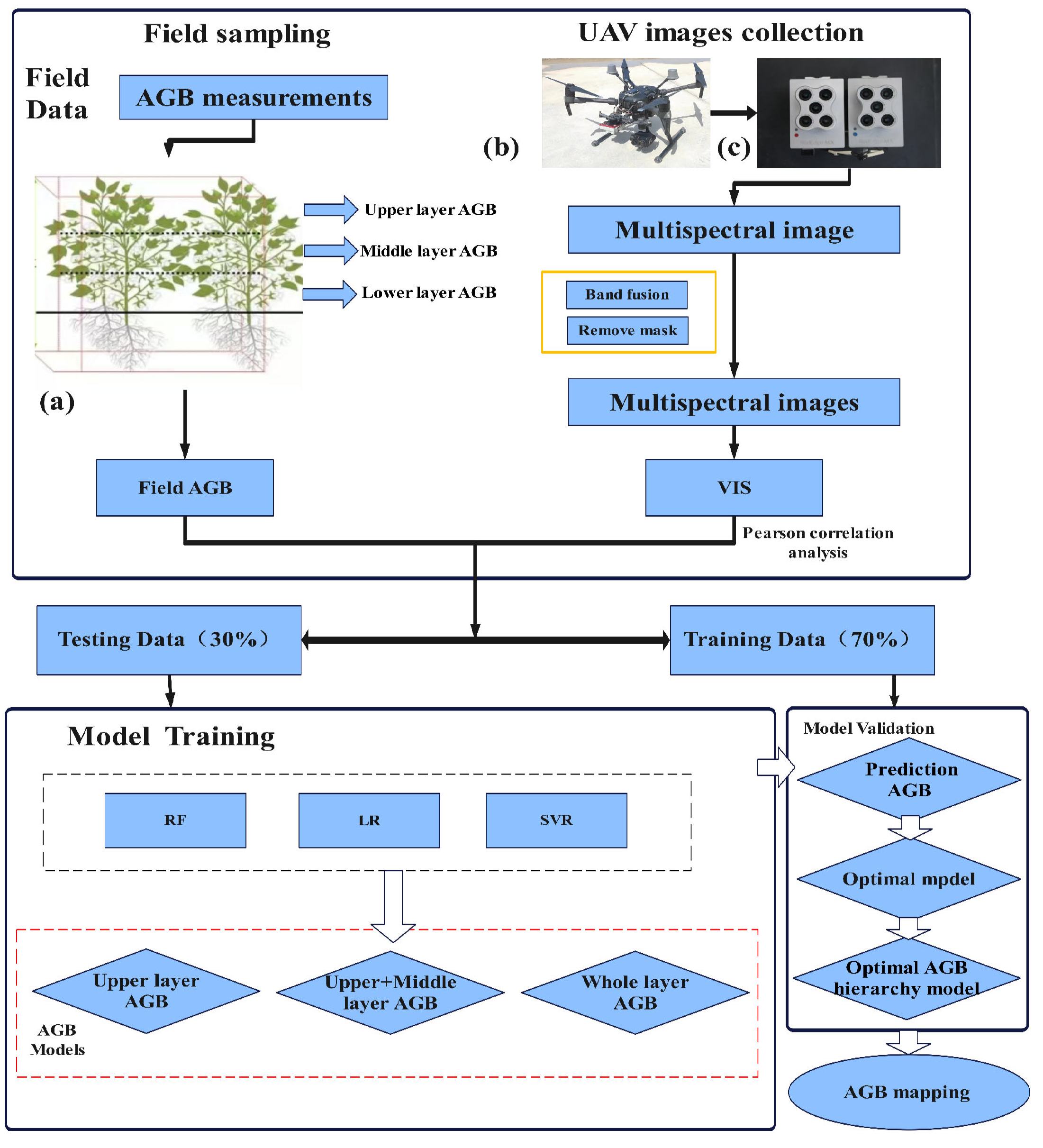
2. Materials and Methods

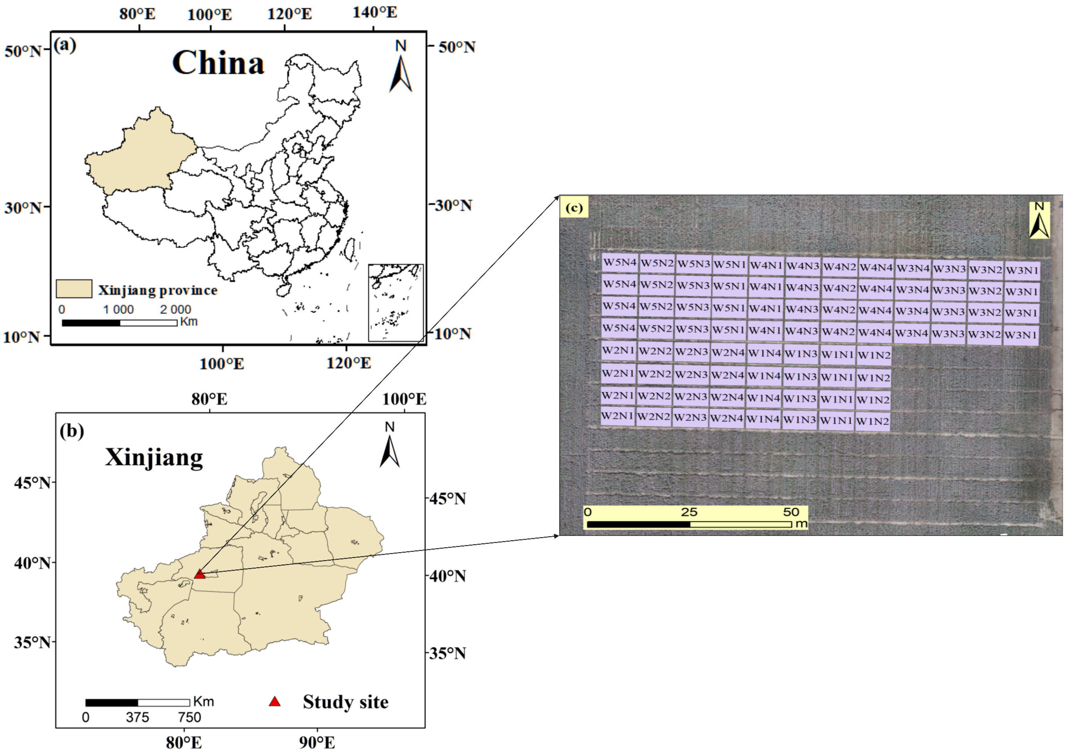
2.1. Overview of the Study Area

The study area is located in Awati County, Xinjiang, China (40°27′ N, 80°21′ E), as shown in Figure 1. The region is characterized by a typical arid continental climate with long sunshine hours, low annual precipitation (approximately 100–150 mm), and high evaporation rates. The region experiences significant temperature variations between day and night, with an average annual temperature of approximately 11.5 °C. The soil type is predominantly gray desert soil with moderate fertility, making it well suited for cotton cultivation. Awati County is known as a major cotton production area in China, contributing significantly to the country’s overall output, and its unique environmental conditions provide an ideal setting for studying crop growth and biomass estimation. (Multispectral images can be seen in Supplementary Material Figure S1).

2.2. Experimental Design

The experiment was conducted from April to October 2023 in a randomized complete block design with four nitrogen application rates (urea, N = 46.4%): 0 kg/hm² (N1), 150 kg/hm² (N2, 0.5× normal rate), 300 kg/hm² (N3, normal rate), 450 kg/hm² (N4, 1.5× normal rate). Additionally, five irrigation treatments were used: 50% (2250 m³/hm², W1), 75% (3150 m³/hm², W2), 100% (4050 m³/hm², W3), 125% (4950 m³/hm², W4), and 150% (5850 m³/hm², W5) of the crop water requirements. Each treatment included three replicates, and each plot measured 49 m² (7.0 m × 7.0 m). The test variety was Xinluzhong 88, and the cotton was sown on April 7 under drip irrigation with plastic film mulch. The experimental field had sandy loam soil, and the previous crop was cotton. The row spacing was 76 cm, the plant spacing was 5.5 cm, and the planting density was approximately 239,000 plants/ha. Basal fertilizer accounted for 20% of the total nitrogen application, while phosphorus and potassium fertilizers were applied as diammonium phosphate (P₂O₅ ≥ 42%, N ≥ 15%) and potassium sulfate (K₂O ≥ 57%) at rates of 257 kg/hm² and 142 kg/hm², respectively. Standard agronomic practices were implemented for field management.

2.3. UAV Data Acquisition

Data collection was conducted at four key growth stages: bud stage, flowering stage, boll setting stage, and boll opening stage. UAV-based multispectral imaging was used to monitor plant height and AGB, while ground-truth measurements were collected to validate UAV-derived data. To minimize weather-related variability, the data collection was performed on sunny and windless days, with UAV imaging was conducted between 12:00 and 14:00 and ground data collected between 8:00 and 12:00 (specific dates are shown in

Table 1. Date of UAV flight acquisition.

Date of Flight	Date of Field Sampling	Growth Stages
06-12	06-12	Bud stage
07-08	07-08	Flowering stage
08-09	08-09	Boll setting stage
09-02	09-02	Boll opening stage

).

2.4. Ground-Truth Data Collection

For ground-based measurements, six cotton plants were randomly selected from each plot to measure plant height, with the average value calculated to represent the plot-level measurement. AGB was determined by measuring the fresh weight of the aboveground cotton shoots immediately after sampling using a precision electronic balance (±0.1 g). During each UAV flight campaign, AGB samples were collected to validate the remote sensing measurements. Sampling was conducted across six plant quadrats randomly distributed within the plots, ensuring representation of the upper, middle, and lower canopy layers. Fresh biomass was measured immediately after collection, and the samples were then oven-dried at 105 °C in a forced-air oven for 48 h to obtain the dry biomass values. These measurements provided a comprehensive dataset for model training and evaluation.

2.5. Vegetation Indices and Feature Extraction

2.5.1. Spectral Image Acquisition

Spectral image acquisition was conducted under clear sky conditions using a Matrice M210 RTK V2 drone with an RGB visible digital camera Zenmuse XT2 (DJI Technology Co., Shenzhen, China), and a multispectral camera (MicaSense, Seattle, WA, USA). The details of the multispectral sensor are shown in Figure 2 and

Table 2. Spectral bands of the MicaSence RedEdge multispectral camera.

Number of Channels	Channel Name	Central Wavelength/nm	FW HM/nm
1	Blue1	444	28
2	Blue2	475	32
3	Green1	531	14
4	Green2	560	27
5	Red1	650	16
6	Red2	668	14
7	Red Edge1	705	10
8	Red Edge2	717	12
9	Red Edge3	740	18
10	NIR	842	57

. The flight route was designed with a mission height of 30 m, a course overlap rate of 75%, a side overlap rate of 75%, and a flight speed of 2 m/s. Images were captured at equal intervals, with a photo interval of 2 m. Geometric correction was performed using ground control points, and flight operations were autonomously managed using DJI Pilot software (DJI Technology Co., Shenzhen, GD, China). To ensure radiometric consistency, images of the built-in radiometric calibration panel were taken before take-off and after landing for calibration during image processing (The multispectral sensor parameters can be found in Table S1 in the Supplementary Material).

2.5.2. Spectral Image Preprocessing

Multispectral stitching and radiometric calibration were performed with the help of Pix4D mapper software (version 4.5.6, Pix4D S.A., Prilly, CH, Switzerland) was used to georeference the stitched images to facilitate batch processing. Since the image contains areas other than the test area, it is necessary to draw a mask file of the test plot and superimpose it on the registered spectral image to extract all the test plots in batches.

2.5.3. Spectral Index Processing

The ten-channel multispectral sensor used in this study captures reflectance data across multiple spectral bands. To address potential multicollinearity among spectral bands and enhance model robustness, the entropy weight method was employed to assign optimal weights to each spectral band. The details are as follows:

Matrix standardization. Due to the different dimensions between the dimensions of the sample matrix X, it is necessary to standardize the original data to obtain the standardized matrix R = (r_ij)nxm. There are two ways to normalize the data: when the indicator data are as large as possible, that is, when it is a positive indicator, the standardized formula is Equation (1), and when the indicator data are as small as possiblethat is, the inverse indicator, the standardized formula is Equation (2). The specific formulas are as follows:

$$r_{ij}={\displaystyle \frac{x_{ij}-x_{min,j}}{x_{max,j}-x_{min,j}}}$$

(1)

$$r_{ij}={\displaystyle \frac{x_{max,j}-x_{ij}}{x_{max,j}-x_{min,j}}}$$

(2)

r_ij is the observation of the jth index of the ith sample after normalization.

Calculation of the entropy value. Firstly, the values of each index are normalized, and the proportion of the index value of the ith evaluation object under the jth index is calculated:

$$r_{ij}={\displaystyle \frac{x_{max,j}-x_{ij}}{x_{max,j}-x_{min,j}}}$$

(3)

Then, the entropy of the j-th indicator is calculated:

$$P_{ij}={\displaystyle \frac{r_{ij}}{\sum _{i=1}^n{r}_{ij}}}$$

(4)

Calculation of entropy weights. After obtaining the entropy value of the jth index, the difference coefficient and entropy weight can be obtained: α_j ω_j.

$${\alpha }_j=1-H_j$$

(5)

$${\omega }_j={\displaystyle \frac{1-H_j}{n-\sum _{i=1}^n{H}_j}}={\displaystyle \frac{{\alpha }_j}{\sum _{i=1}^n{\alpha }_j}}$$

(6)

2.5.4. Spectral Index Extraction

The VIs refers to the enhanced vegetation information formed by the combination of bands, reflecting the difference between the reflection of vegetation in the visible light, near-infrared, and other wavebands and the soil background. The construction of the VIs can realize the quantitative expression of the vegetation growth status. It is calculated by combining multiple bands in the spectrum, and has better sensitivity than a single band in measuring the state of ground vegetation [18]. In recent years, with the popularization of hyperspectral imaging, many VIs have been used as predictors of the AGB, leaf area index, and yield of cotton, potato, and other crops [1,19]. In this study, 20 VIs (

Table 3. Formulas for calculating vegetation indices.

Vegetation Index	Calculation Formula	Reference
Normalized Vegetation Index (NDVI)	$(NIR-R)/(NIR+R)$	[20]
Normalized Red-edged Vegetation Index (NNIR)	$(NIR-RE)/(NIR+RE)$	[21]
Ratio Vegetation Index (RVI)	$NIR/R$	[22]
Difference Vegetation Index (DVI)	$NIR-R$	[23]
Wide Dynamic Vegetation Index (WDRVI)	$(0.2\ast NIR-R)/(0.2\ast NIR+R)$	[24]
Green Vegetation Index (GRVI)	$NIR/G$	[22]
Green Normalized Difference Vegetation Index (GNDVI)	$(NIR-G)/(NIR+R)$	[25]
Blue Normalized Difference Vegetation Index (BNDVI)	$(NIR-B)/(NIR+B)$	[25]
Green Difference Vegetation Index (GDVI)	$NIR-G$	[26]
Enhanced Vegetation Index (EVI)	${\displaystyle \frac{2.5\ast (\mathrm{N}\mathrm{I}\mathrm{R}-\mathrm{R})}{(\mathrm{N}\mathrm{I}\mathrm{R}+6\ast \mathrm{R}-7.5\ast \mathrm{B}+1)}}$	[27]
Structurally insensitive pigment index 2 (SIPI2)	$(\mathrm{N}\mathrm{I}\mathrm{R}-\mathrm{G})/(\mathrm{N}\mathrm{I}\mathrm{R}-\mathrm{R})$	[28]
Soil-Conditioned Vegetation Index (SAVI)	$(1+\mathrm{L})(\mathrm{N}\mathrm{I}\mathrm{R}-\mathrm{R})/(\mathrm{N}\mathrm{I}\mathrm{R}+\mathrm{R}+\mathrm{L})$	[29]
Optimized Soil-Conditioned Vegetation Index (OSAVI)	$1.16\ast (\mathrm{N}\mathrm{I}\mathrm{R}-\mathrm{R})/(\mathrm{N}\mathrm{I}\mathrm{R}+\mathrm{R}+0.16)$	[29]
Generalized Optimized Soil-Regulated Vegetation Index (GOSAVI)	$1.16\ast (NIR-G)/(NIR+G+0.16)$	[30]
Green Chlorophyll Index (CIGreen)	$NIR/G-1$	[27]
Red Edge Simple Ratio (RESR)	$RE/R$	[31]
Atmospheric Impedance Vegetation Index (ARVI)	(NIR − 2 ∗ R + B)/(NIR + B)	[32]
Triangular Vegetation Index (TVI)	$\sqrt[2]{0.5+(NIR-R)/(NIR+R)}$	[27]
GreenRed Difference Vegetation Index (GRDVI)	$(NIR-G)/\left(\sqrt[2]{(NIR+G)}\right)$	[30]
Improved Simple Odds Index (MSR)	($NIR/R-1)/(\sqrt[2]{(NIR/R)+1)})$	[33]
Generalized Improved Simple Odds Index (GMSR)	$(NIR/G-1)/\left(\sqrt[2]{(NIR/G)+1)}\right)$	[30]

Note: NIR, R, B, G, and RE are the reflectances of the near-infrared, red, blue, green, and red-edge bands, respectively, which are weighted using the entropy weight method.

) with a good correlation with AGB and the cotton crop were selected based on previous studies. Then, several VIs with the highest correlation were screened out using a Pearson correlation analysis of cotton’s AGB, and the vegetation indices with the strongest correlation were combined with the AGB data for modeling and inversion map construction.

2.6. Model Selection

In this study, the vertical distribution of stratified biomass in oasis cotton fields was determined by utilizing UAV-based multispectral remote sensing. Experiments were conducted using a UAV equipped with a 10-channel multispectral sensor to collect spectral reflectance data from cotton fields at different growth stages, and three algorithms were applied to estimate linear gradient regression, which improves model performance by gradually optimizing residuals. Finally, vector regression was supported to find the optimal hyperplane with the smallest deviations in the data. The combination of these methods aims to improve the accuracy and efficiency of cotton biomass estimation and provide a scientific basis for precision agriculture management.

2.7. Statistical Analysis

The samples were randomly divided into a training set and a test set of the model at a ratio of 7:3, with cotton AGB as the target variable and the feature set pre-selected by the feature selection algorithm as the input variable for building the model. Based on the Python (3.9.13) environment, the scikit-learn (1.1.1) package implements three modeling algorithms: the SVM, RF, and linear regression gradient boosting model. In this study, the decision tree depth, number of iterations, and other hyperparameters of the stochastic Mori Ridge regression model were fine-tuned using a 5-fold cross-validated grid search method, and the rest of the model parameters were used by default.

The coefficient of determination (R²) was used to evaluate the fitting effect of the model, and the root mean square error (RMSE) was used to evaluate the effectiveness of different models. The higher the R² value, the better the model fit, and the smaller the RMSE value, the smaller the model error and the stronger the model generalization ability.

$$R^2={\displaystyle \frac{{\sum }_{i=1}^n{\left(x_i-\overline{x}\right)}^2{(y_i-\overline{y})}^2}{{\sum }_{i=1}^n{\left(x_i-\overline{x}\right)}^{2}n{\sum }_{i=1}^n{(y_i-\overline{y})}^2}}$$

(7)

$$\mathrm{R}\mathrm{M}\mathrm{S}\mathrm{E}=\sqrt{{\displaystyle \frac{1}{n}}{\sum }_{i=1}^n{(y_i-x_i)}^2}$$

(8)

where n is the sample size, i is the datapoint of the ith sample, x_i is the measured value of the ith sample, x is the average value of the measured value, y_i is the predicted value of the ith sample, and y is the average value of the predicted value. Figure 2 shows the technical flow of this paper.

Figure 2. Experimental methods and statistical analysis process in this study. (a) Vertical layering of cotton. (b) Matrice M210 RTK V2 (DJI Inc., Shenzhen, China) UAV. (c) 10-channel multispectral sensor RedEdge-MX-Dual (Micasense Inc., Seattle, WA, USA).

Figure 2. Experimental methods and statistical analysis process in this study. (a) Vertical layering of cotton. (b) Matrice M210 RTK V2 (DJI Inc., Shenzhen, China) UAV. (c) 10-channel multispectral sensor RedEdge-MX-Dual (Micasense Inc., Seattle, WA, USA).

3. Results

3.1. Cotton Biomass Analysis

Through the analysis of the layered AGB data of cotton at different growth stages (

Table 4. Statistical characteristics of stratification and biomass of different organs of cotton at four growth stages.

Reproductive Period	Level	Sample Size (pcs)	Mean (g/cm2)	Min (g/cm2)	Max (g/cm2)	Standard Deviation	Coefficient
Bud stage	upper	60	3.46	2.55	4.96	0.37	0.11
	middle	60	3.05	2.24	3.60	0.35	0.11
	lower	60	2.37	1.60	3.38	0.37	0.15
Flowering stage	upper	60	15.09	9.72	20.06	2.61	0.17
	middle	60	12.34	8.52	17.59	2.09	0.17
	lower	60	4.50	1.56	9.32	1.46	0.33
Boll setting stage	upper	60	15.46	8.50	26.59	3.90	0.25
	middle	60	11.49	7.60	20.88	2.46	0.21
	lower	60	32.47	18.51	48.50	6.82	0.21
Boll opening stage	upper	60	15.63	9.34	23.79	4.00	0.26
	middle	60	11.20	5.73	17.63	2.61	0.23
	lower	60	45.02	21.90	65.41	9.76	0.22

), the growth, development, and nutrient distribution characteristics of cotton are clear. At the bud stage, the average AGB of the upper, middle, and lower layers of cotton was 3.46 g, 3.05 g, and 2.37 g, respectively, with a low coefficient of variation. However, the reproductive organs had a higher coefficient of variation (0.52), indicating uneven development. At the flowering stage, the average AGB of the upper, middle, and lower layers increased significantly, reaching 15.09 g, 12.34 g, and 4.50 g, respectively. The average dry weight of the vegetative organs and reproductive organs was 21.44 g and 11.94 g, respectively, and the coefficient of variation of reproductive organs remained high (0.469). At the boll setting stage, the average dry weight of the upper, middle, and lower layers continued to increase, and was 15.46 g, 11.49 g, and 32.47 g, respectively, and the average dry weight of the vegetative and reproductive organs reached 40.96 g and 19.60 g, respectively. At the flocculation stage, the average dry weight of the upper, middle, and lower layers of the cotton was 15.63 g, 11.20 g, and 45.02 g, respectively, and the average dry weight of the vegetative organs and reproductive organs was 45.66 g and 29.11 g, respectively, indicating that the nutrient distribution was relatively uniform. In general, the coefficient of variation of the biomass at different growth stages was mostly less than 30%, indicating that the nutrient distribution of the cotton in each sampling area was relatively uniform, while the coefficient of variation of the reproductive organs was higher, indicating the imbalance in their development process. Through the analysis of these data, it is possible to better understand the characteristics of the cotton biomass changes at different growth stages and their impact on productivity.

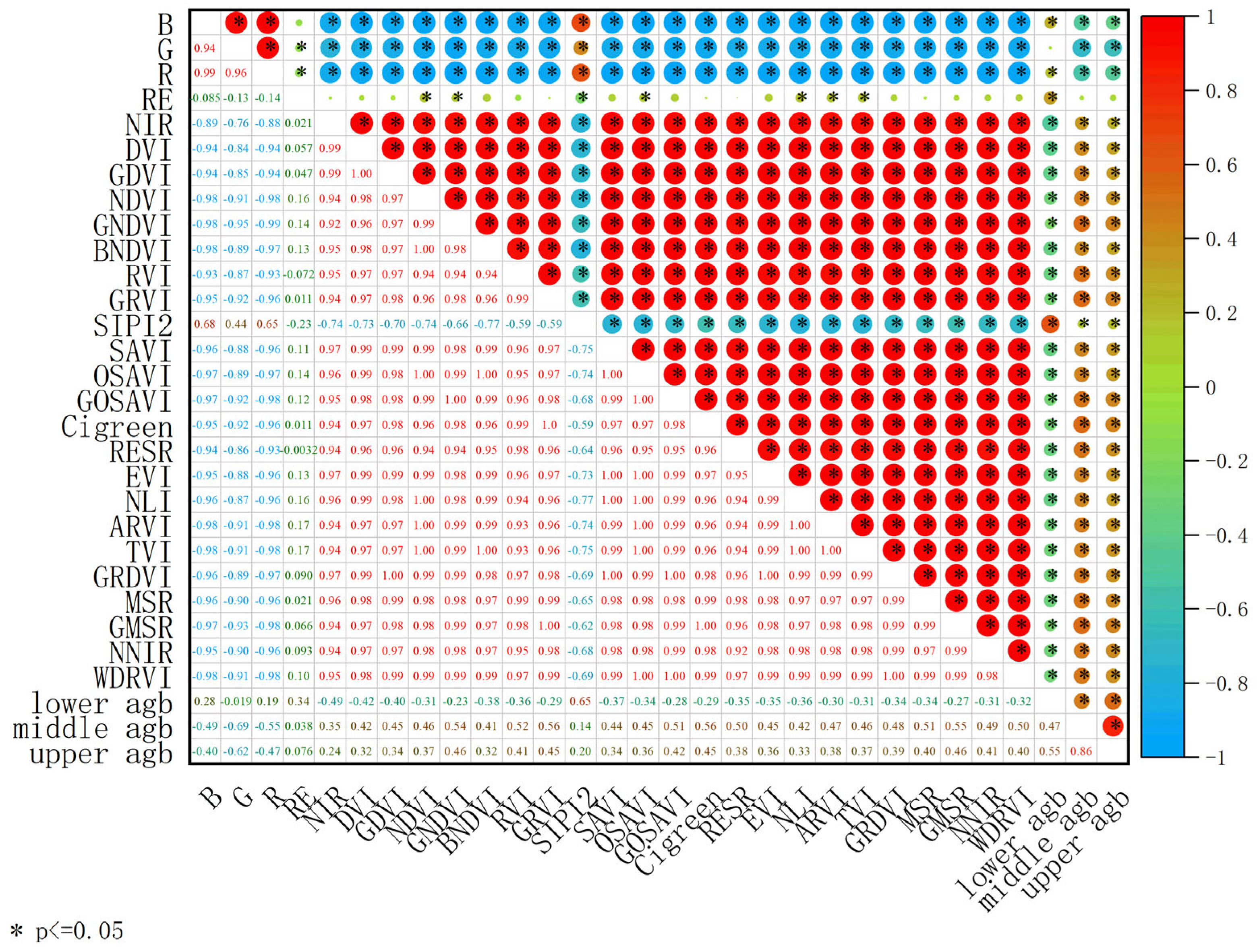
3.2. Correlation Analysis of AGB of Cotton Based on Pearson

A correlation analysis between the spectral characteristics of the cotton canopy and the AGB was carried out, and the results are shown in Figure 3. All vegetation indices were significantly positively correlated with Upper-AGB and Middle-AGB, negatively correlated with Lower-AGB, and only positively correlated with SIPI2. The blue, green, red, and red-edge bands were significantly negatively correlated with the AGB. The spectral characteristics with a high correlation with Upper-AGB were G and NIR, and their correlation coefficients were −0.62 and 0.32. The spectral characteristics with a high correlation with Middle-AGB were G and NIR, and their correlation coefficients were −0.69 and 0.452. The spectral features with a high correlation with Lower-AGB were RESE and NIR, with correlation coefficients of 0.34 and −0.49.

The spectral characteristics of five band images of the cotton canopy, processed using the entropy weight method, were calculated, and a correlation analysis was carried out with the AGB of each layer. As shown in Figure 3, SIPI2 was significantly positively correlated with Lower-AGB (r = 0.65, p < 0.001) and negatively correlated with DVI and GDVI (p < 0.001). The characteristics GNDVI, GRVI, Cigreen, RESR, MSR, GMSR, and GMSR were significantly positively correlated with Middle-AGB (r > 0.50, p < 0.001). There was a significant positive correlation between GNDVI, GRVI, Cigreen, and GMSR (r > 0.45, p < 0.001), and the correlation coefficient between GRVI and Cigreen was the highest with these two levels of AGB.

3.3. Vegetation Index Was Used to Estimate Cotton Biomass at Different Growth Stages

3.3.1. Data Division

The samples screened in the four periods were divided into a training set and test set in a ratio of nearly 7:3. A total of 60 samples were screened at each fertility stage, of which 42 were used in the training set and 18 were used in the test set.

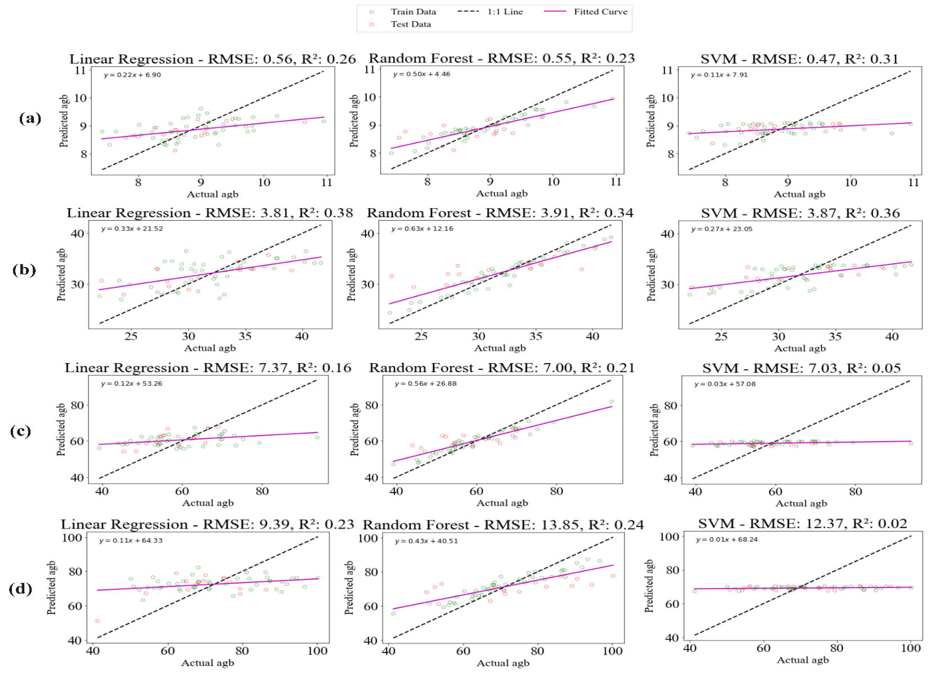
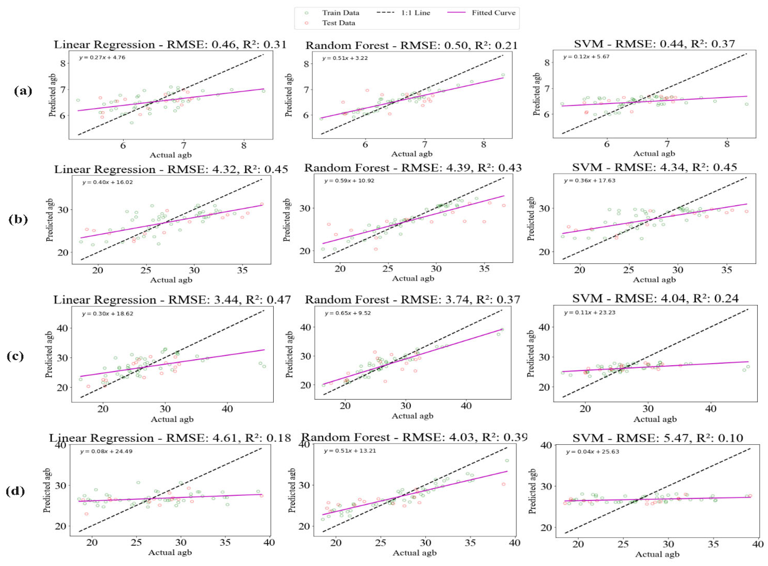
3.3.2. Construction of Upper, Middle, and Lower Inversion Models

In the study of AGB inversion modeling over periods with different levels of cotton growth, our research team applied three algorithm models: RF, LR, and SVR. These algorithms were used to select the characteristics of the cotton AGB, and the importance of the characteristics of the AGB in cotton was evaluated. The spectral characteristic variables with low importance were first excluded, and then the cotton AGB was modeled according to the spectral characteristic variables. Comparing the four growth stages (Figure 4), the three models had slightly better results at only the bud stage and flowering stage, with the highest R² and the lowest RMSE of 3.81 in the LR model. The three models showed different effects in the middle and late stages of growth, where LR and RF showed a slight decrease in R² at the boll setting stage and flocculation stage and SVM decreased greatly, where the R² was as low as 0.02, indicating that the applicability of any model was poor in the middle and late stages of cotton growth. In order to improve the problem of low accuracy in the middle and lower layers of the model, this study divided the cotton field into upper, middle, and lower levels, combined them with ML modeling, and compared how the accuracy of the model and the use of the three levels changed.

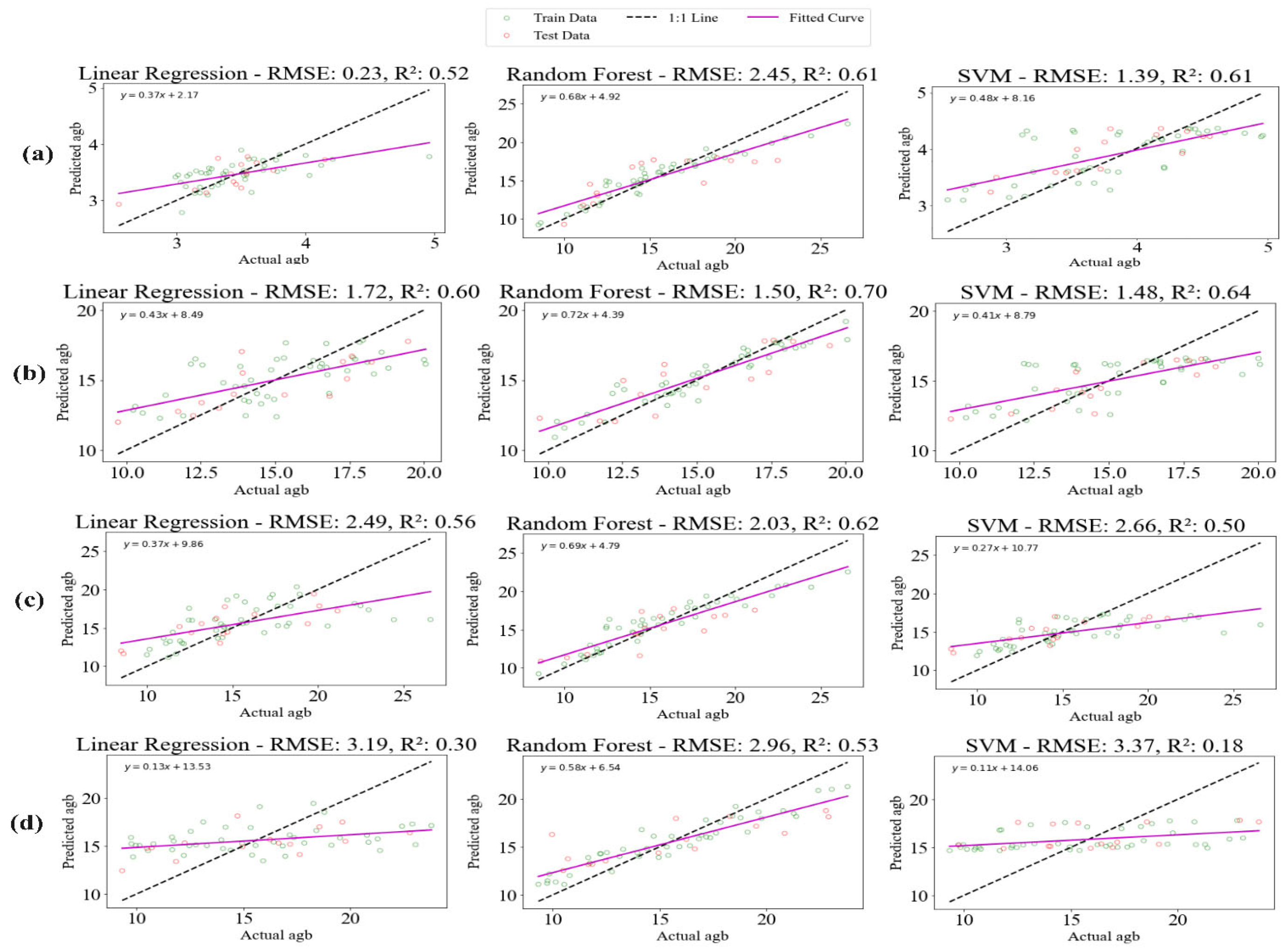
3.3.3. Construction of Upper- and Middle-Level Inversion Models

Figure 5 shows the results of the spectral upper and middle layers of the AGB model of cotton, which showed a certain improvement in prediction accuracy compared with the whole plant model. The accuracy of the model constructed using the whole AGB was poor at the boll setting stage and flocculation stage, which was related to the weak penetration ability of the UAV, as well as the fact that the pictures taken by the UAV could not fully and effectively reflect the biomass composition of the middle layer of the cotton, which was consistent with common sense. In the middle and late stages of cotton growth, the cotton structure became more complex and the canopy was more closed, resulting in a great decrease in drone penetration, so the prediction accuracy of several models was also greatly reduced. To improve the accuracy of the model in estimating cotton, a new model was constructed by combining the upper cotton biomass with the middle cotton biomass, and the three new models were defined as Upper- and Middle-LR, Upper- and Middle-RF, and Upper- and Middle-SVM (Figure 5). At the bud and flowering stages, the R² using the three new models increased by about 10–33%, and the accuracy of the AGB estimation was higher. The estimation of biomass was significantly improved by the improved model, especially during the boll setting stage, where the Upper- and Middle-LR model increased by 0.31 compared with the Whole-LR model R²; the Upper- and Middle-RF model increased by 016. Compared with the original model R², the Upper- and Middle-SVM model increased by 0.19, which shows that the three models can more effectively predict the whole plant biomass of cotton after the introduction of cotton biomass in the upper layer. The nonlinear models (RF and SVM) fit AGBs better than the linear models (LR). Compared with SVM, RF is more stable, the model error is lower, and the RMSE is lower.

3.3.4. Construction of Upper-Layer Inversion Model

Figure 6 shows the results of a spectroscopy-based AGB model for the upper layer of cotton. The experimental results show that the model constructed with the upper AGB provides a significant improvement in model accuracy and performance. Compared with the traditional whole-plant AGB model, the R² using only the upper biomass was increased by 100%, while the Upper-RF did not improve, probably because the RF required a large sample data size. At the flowering stage, the RF model showed an excellent fitting ability for the estimation of the upper biomass at the flowering stage of cotton, with the highest R² value of 0.7 and the lowest RMSE of 1.5, indicating that RF performed well in capturing the complex relationship of the training data. The performance of LR and SVM was slightly worse than that of RF, with R² values of 0.6 and 0.64, respectively, and the three new models improved their R² by 58%, 105%, and 78%, respectively, compared with the whole AGB model. In the bell period, the performance of the three new models modeled with upper-level AGB was significantly improved, and the R² of the three models of Upper-LR, Upper-RF, and Upper-SVM was increased by 19%, 68%, and 108% compared with that of Upper- and Middle-LR, Upper- and Middle-RF, and Upper- and Middle-SVM, respectively, and the RMSE of Upper-RF was 2.03, which was the best among the three models. In the flocculation period, the three new models also improved to a certain extent compared with the models modeled by the upper and middle AGB, with R² increasing by 0.12, 0.18, and 0.08, respectively, and the performance of Upper-RF still being the best, where its R² was as high as 0.53 and RMSE was 2.96. The Upper-SVM was also slightly improved in the flocculent period. This indicates that the RF model has a strong fitting ability for different organs of cotton (The residual analyses of the models can be seen in Figure S2 in the Supplementary Material).

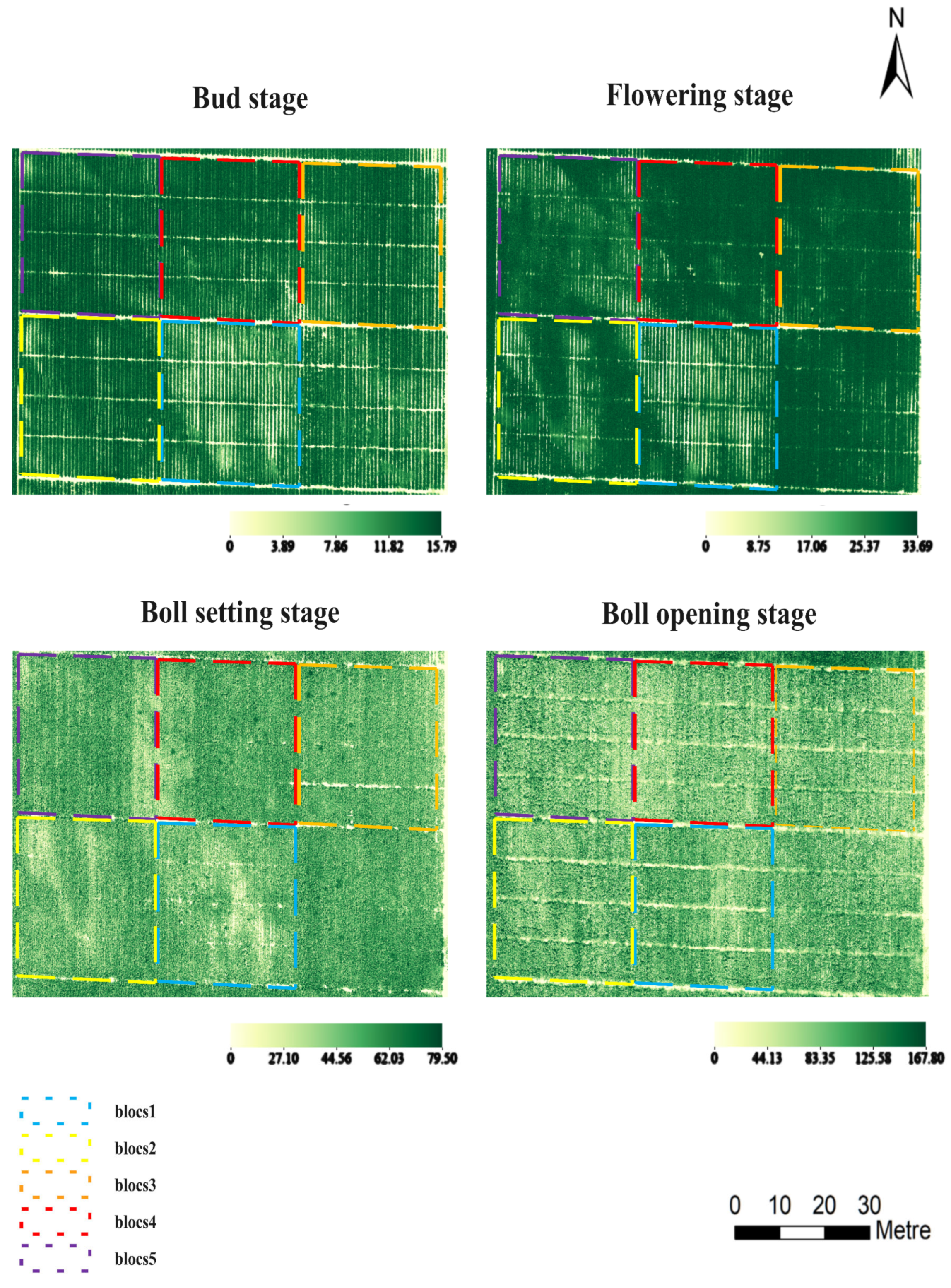
3.4. Above-Ground Biomass Inversion Mapping

Figure 7 shows the AGB inversion spectrum of cotton at different growth stages. The inversion maps were plotted at the pixel level, and the physical length of each pixel was 2 cm. As shown in Figure 7, the darker the color of the inversion map for each period, the higher the quality of the plot to which it belongs. At DAS 58, most of the cotton plants were in the bud stage, and the cotton plants were relatively small. The average AGB of the cotton was 8.88 g/cm². At DAS 84, most of the cotton plants were in the flowering stage, and the average AGB of the cotton was 31.93 g/cm². After rapid growth, the AGB value mainly ranged from 22.23 g/cm² to 41.63 g/cm². At DAS 116, most of the cotton plants were in the boll setting stage. The average AGB of the cotton reached 60.56 g/cm². At DAS 140, most of the cotton plants were in the flocculation stage. The average AGB of the cotton was 71.85 g/cm².

4. Discussion

As an important cash crop, the biomass estimation of cotton during its growth process is of great significance for optimizing agricultural management and increasing yield. Traditional biomass estimation methods often rely on single spectral information and simple statistical models, which often show great limitations in dealing with the complex and dynamic processes of crop growth, especially the stratified biomass estimation of different growth periods and different plant organs. With the advancement of remote sensing technology, multispectral remote sensing provides a richer data source for crop biomass estimation, especially the high-resolution multispectral images obtained through the UAV platform, which can more accurately capture the spectral characteristics of crops at different growth stages.

4.1. Estimation of AGB in Vertical Distribution of Cotton Based on Spectral Characteristics

This study introduces a stratified modeling approach to estimate the vertical distribution of cotton AGB utilizing UAV-based multispectral remote sensing. The results highlight significant spectral reflectance differences across the upper, middle, and lower canopy layers (p < 0.05), with the upper canopy showing the strongest sensitivity to AGB (R² = 0.70 at the flowering stage). The stratified model greatly improved estimation accuracy during the middle-to-late growth stages (boll setting and opening), achieving a maximum R² increase of 0.45 and reducing RMSE by 40% compared to the traditional whole-plant models (Figure 4, Figure 5 and Figure 6). These findings surpass those of Li et al. [1], who employed UAV hyperspectral data for potato AGB estimation but neglected canopy stratification, leading to NDVI saturation under high-biomass conditions (R² dropped to 0.48). In comparison, this study achieved a more significant improvement (R² = 0.55), underscoring the efficacy of stratified models for crops with complex canopy architectures. The results contribute new insights into precision monitoring for high-biomass crops like cotton and sugarcane. Stratified approaches help optimize resource management, such as refining nitrogen applications in dense upper foliage to enhance resource-use efficiency. Additionally, this method compensates for UAV limitations in penetrating dense canopies, offering practical benefits for large-scale field monitoring.

However, this study is limited by the use of a 10-channel multispectral sensor with limited spectral resolution, which may hinder the detection of biochemical parameters like chlorophyll fluorescence, especially when compared to hyperspectral systems [10]. The data acquisition was restricted to clear-sky conditions, which may have affected the model’s generalizability due to spectral fluctuation challenges under cloudy conditions [30]. In conclusion, this research emphasizes the critical role of vertical canopy stratification in cotton AGB estimation, demonstrating how stratified modeling effectively mitigates the saturation issues observed in conventional methods. Despite sensor and weather constraints, this approach offers a cost-effective, high-accuracy solution for dynamic monitoring in precision agriculture.

4.2. Advantages of Constructing AGB Estimation Model for Upper and Middle Layers of Cotton

This study developed stratified models for estimating cotton AGB in the upper and middle canopy layers, which significantly improved prediction accuracy during its high-biomass stages. The upper-layer model (Upper-RF) achieved R² values of 0.70 (flowering) and 0.53 (boll setting stage), with the RMSE reduced to 1.5 g/cm² and 2.03 g/cm², respectively, outperforming the whole-plant models by 58% in R² (Figure 6). The combined upper model (Upper-RF) addresses UAV penetration limitations. This approach outperforms previous methods in maize LAI estimation [33] and soybean modeling [34], reducing RMSE by 51% through improved spectral saturation handling and canopy structural complexity resolution. Additionally, entropy-weighted spectral indices enhanced training efficiency by 30% compared to the texture-based models used in rice (Xu et al., 2022) [7], demonstrating superior feature optimization.

Stratified modeling has practical applications in precision agriculture, including guiding nitrogen reduction in high-biomass upper canopies (R² > 0.65) and optimizing irrigation through middle-layer estimates (RMSE < 2.5 g/cm²). However, the reliance on specific red-edge bands (705–740 nm) may overlook subtle chlorophyll signals [10], and the clear-sky data requirements (illumination > 1000 W/m²) may limit applicability in variable climates [30]. Future improvements should focus on integrating LiDAR-derived 3D point clouds [9] for enhanced vertical resolution, employing attention mechanisms (e.g., Transformer) for dynamic feature weighting, and validating cross-crop adaptability [29].

In conclusion, stratified modeling significantly improves cotton AGB estimation accuracy (ΔR² > 0.55) during its mid-to-late growth stages. Despite the challenges posed by sensor and climatic constraints, this approach provides a cost-effective and scalable framework for precision agriculture in complex canopies, balancing technical feasibility with practical applicability.

4.3. Differences in and Advantages of the New Model

The proposed stratified model enhances the robustness of cotton AGB estimation in complex canopy environments by incorporating a dynamic feature weighting mechanism and a cross-layer data fusion strategy. Compared to traditional whole-plant models, this model achieved a 0.45 improvement in R² during the mid-to-late growth stages (Figure 5). The model also demonstrated improved tolerance to spectral fluctuations under cloudy conditions, with the RMSE increasing by only 12% under ±20% illumination variations, compared to a 28% increase for conventional models.

The model’s innovations lie in two main areas. First, dynamic entropy weighting allows feature weights to adjust according to the canopy growth stages, such as increasing the red-edge band weight to 0.45 during the flowering stage. This boosts R² by 0.18 compared to fixed-weight strategies. Second, the model enhances data fusion efficiency. Unlike methods that use LiDAR to fuse spectra, our model relies only on multispectral data, resulting in significant cost savings. The stratified feature fusion reduces the RMSE to 2.03 g/cm², narrowing the accuracy gap with high-cost LiDAR solutions (RMSE = 1.8 g/cm²) to just 11%. The advantages of the new model have practical value. The model automatically adapts to canopy structural changes by optimizing layer-specific weights. For example, in high-nitrogen treatments, the upper-layer weight increases to 70%, reducing the need for manual parameter tuning. Moreover, hardware costs are reduced by 85% compared to LiDAR-based solutions while maintaining comparable accuracy. This makes the model viable for small- and medium-sized farms. The model also supports seamless integration with satellite data, such as Sentinel-2, providing a foundation for regional-scale AGB monitoring. Despite these advancements, the model has limitations. Real-time constraints exist due to offline layer-specific feature extraction, requiring over 15 min per processing cycle, which limits real-time monitoring, indicating that further optimization is necessary for cross-crop generalization. Additionally, the model’s dependency on RTK drone positioning (error < 2 cm) restricts its use in areas without base station coverage. Future work should focus on integrating edge computing to enable lightweight models on drones for real-time, layer-specific feature extraction. Cross-crop transfer learning could be explored to develop a universal stratification framework, adapting pre-trained cotton models to other crops such as sugarcane and maize. Additionally, multi-source data fusion could be explored to compensate for low-precision GNSS (error < 1 m), expanding the model’s applicability.

By integrating dynamic weight allocation and low-cost stratified fusion, this study addresses the saturation issues in high-biomass stages (R² > 0.55) and overcomes the hardware dependency bottlenecks present in traditional models. Despite real-time and generalization constraints, this model offers a precise and practical solution for monitoring crops with complex canopies, laying a strong foundation for multi-scale agricultural remote sensing.

4.4. Effect of Machine Learning Algorithm on AGB Estimation Model of Cotton at Different Levels

This study evaluated the performance of three algorithm models, RF, LR, and SVR, for estimating AGB at different canopy levels (upper, middle, lower) and growth stages in cotton. RF performed the best at estimating AGB in the upper canopy during the flowering and boll setting stages (R² = 0.70, RMSE = 1.5 g/cm²) but exhibited significant overfitting risks during the seedling stage (R² = 0.32) and in the test set (R² dropped to 0.45). The growth stages significantly impacted algorithm performance. LR and SVR performed stably during the seedling and flowering stages (R² > 0.60), but their performance decreased in the later stages (boll and boll opening), with R² dropping by 0.18 and 0.25, respectively, due to increasing canopy complexity. The middle and lower canopy levels presented significant limitations, with all models showing reduced accuracy (R² < 0.40), especially during boll opening (RMSE > 3.5 g/cm²), related to a limited drone penetration capacity and canopy closure.

Compared to existing studies, this research further highlights the dynamic relationship between algorithm selection and crop growth stages. RF’s strengths and limitations were confirmed, consistent with the study of Yang et al. [25] on rice, where RF excelled in processing high-dimensional spectral data. However, RF’s overfitting issue was more pronounced in this study, with a 35% decrease in R² on the test set, likely due to the higher heterogeneity of the cotton canopy. SVR demonstrated greater stability during the seedling, with its resistance to overfitting aligning consistent with finding from soybean study, as the R² on the test set decreased by only 0.08 [28]. However, SVR’s adaptability to complex canopies was weaker compared to the deep learning models [33]. LR showed the best training efficiency (single iteration < 0.5 min). Its decrease in precision (ΔR² = 0.18) was most pronounced in the later stages of the study, indicating that linear models are less effective at capturing nonlinear canopy features. These findings offer practical guidance for algorithm selection in precision agriculture. RF should be prioritized during the flowering stage to maximize accuracy, while LR or SVR should be employed for rapid monitoring in resource-limited scenarios. For the middle and lower canopy layers, multi-angle drone imaging (e.g., oblique photography) should be considered to improve spectral penetration and model robustness. While RF offers high accuracy, its longer training time (300% longer than LR) makes it more suited to research settings, while LR/SVR is better for real-time field monitoring.

This study’s limitations arise from overfitting risks and data dependency. While RF performed well on the training set, it struggled to generalize on the test set, especially under fluctuating environmental conditions (e.g., light changes). Moreover, model performance is highly reliant on high-quality labeled data, and sampling for the middle and lower canopy layers remains difficult due to the challenges of destructive field sampling. Algorithm generalization under extreme climatic conditions (e.g., drought, flooding) remains unverified, which may affect practical applications. Future research could focus on improving algorithm fusion, enhancing data diversity, and optimizing real-time performance. Specifically, combining RF with deep learning (e.g., RF-CNN) could better capture both spectral features and spatial context; synthetic data (e.g., GAN-generated spectra) could address overfitting risks in the middle and lower layers; and edge computing (e.g., TensorRT acceleration) could reduce RF inference time to under 1 min, supporting real-time field monitoring. This study provides a systematic overview of the performance differences and applicability of machine learning algorithms for cotton AGB layer estimation, offering a technical roadmap for dynamic, stratified crop monitoring algorithms.

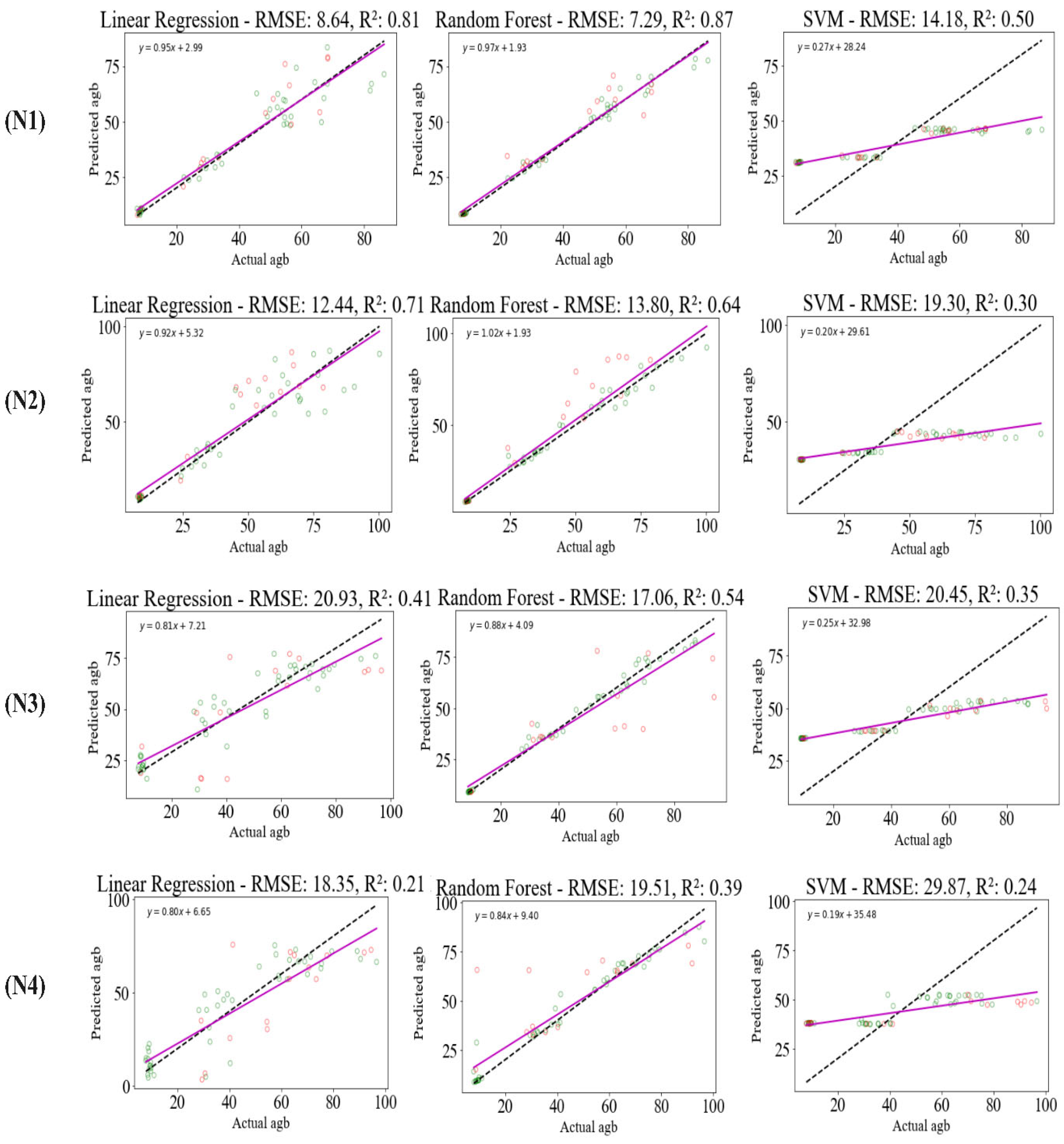
4.5. Effect of Different N Treatments on the Model

From Figure 8, it can be seen that with the increase in N application, the estimation accuracy of AGB by different models shows different effects, but the overall trend is decreasing. When the N level was at a lower level, the R² of the RF model could reach a maximum of 0.87, and the R² of the LR model reached 0.81, which could indicate that these two models had better accuracy in their AGB predictions under the condition of low nitrogen. When the nitrogen was increased to 300–450 kg/hm², the model’s accuracy was significantly reduced, probably due to the promotion of N to the cotton leaves, which made the canopy more depressed, resulting in a significant reduction in the penetration ability of the drone, from which it can be inferred that the lower the N, the stronger the cotton AGB monitoring ability of the drone, though this is not a favorable thing for agricultural production. Therefore, this study does not recommend the use of high nitrogen since the use of a drone to monitor the AGB in cotton fields to improve cotton yield is of great significance. From this, the model constructed by the traditional whole-plant AGB still has the problem that it is greatly affected by canopy closure and spectra, and the model constructed by the two new methods can effectively improve these problems to a certain extent.

4.6. Directions for Improving the AGB Estimation Model

In order to optimize the predictive ability of spectral data for crop AGB, Deery et al. [34,35] found that the predictive accuracy of crop AGB could be effectively improved by introducing ensemble spectral data from elevation data. Tan et al. found that a rubber biomass estimation model constructed using multispectral combined with a deep convolutional neural network (DCNN) (R² = 0.89, RMSE = 6.44 t/ha, MAE = 5.72 t/ha) performed better than a regression model such as random forest (RFR) (R² = 0.81, RMSE = 11.63 t/ha, MAE = 9.27 t/ha) [36]. Follow-up studies could increase the amount of data and introduce deep learning to improve the deep AGB model for cotton. Jing et al. found that the model constructed by combining data measured by UAV-mounted LiDAR with spectral indices could better estimate the AGB of oilseed rape (R² = 0.81) [36], and that LiDAR had a better penetration ability for complex canopy crops, which could subsequently be combined with LiDAR to optimize the layered cotton AGB model for better accuracy and applicability.

Previous studies have shown that significantly outperformed the regression model based on spectral data by constructing a winter wheat and maize (VGC-AGB) model (R² = 0.92 ~ 0.93, RMSE = 68.82 ~ 75. 15 g/m²) [18]. The upper AGB model studied in this article better predicts the AGB composition of this crop at different time subsets compared to winter wheat and maize, which are crops in which the reproductive organs and the stem leaves are not at the same level. Therefore, future research is needed to validate the feasibility of the upper AGB model by combining elevation data, deep learning, and LiDAR. In the future, LIDAR or hyperspectral imaging can be used to further study the complex canopy, and the vertical structure of crops can be analyzed by LIDAR and compared with the method in this paper to optimize the model. This method lays a solid foundation for improving the accuracy of remote sensing models through vertical hierarchical research, thereby contributing to the advancement of digitalization and precision agriculture.

5. Conclusions

Based on UAV remote sensing multispectral images, this study divided cotton into three different layers; studied the distribution and composition factors of AGB in the upper, middle, and lower layers; combined it with ML algorithms to model and compare the AGB of cotton throughout the growth period; and carried out more accurate monitoring. Through the study of the vertical structure of cotton, it was found that the model constructed using any level of AGB had the best performance in the cotton flowering stage, among which the random forest RF model performed the best (R² = 0.7). The accuracy of the model constructed using the wholeplant AGB combined with the three algorithm models showed a significant decrease in the middle and late stages of cotton growth (R² < 0.3), while the model constructed using the upper- and middle-layer AGB combined with the ML algorithms showed a significant improvement in monitoring accuracy during the cotton boll setting stage and flocculation stage. The LR model’s accuracy was the highest in the boll phase (R² = 0.47), and the model accuracy was the highest in the RF phase (R² = 0.39). If only the upper AGB combined with the three algorithms were used to construct the model, the whole growth period of cotton was greatly improved, and the improvement was greater in the middle and late stages, except for the flocculation stage. The R² of the three models in the other growth stages was greater than 0.5, showing good model accuracy and model applicability. Compared with the commonly used methods such as LIDAR and hyperspectral cameras to monitor AGB during the whole growth period of crops, this method greatly saves costs and provides a new idea and method for the low-cost monitoring of other crops.

References

1. Li, B.; Xu, X.; Zhang, L.; Han, J.; Bian, C.; Li, G.; Liu, J.; Jin, L. Above-ground biomass estimation and yield prediction in potato by using UAV-based RGB and hyperspectral imaging. ISPRS J. Photogramm. Remote Sens. 2020, 162, 161–172. [Google Scholar] [CrossRef]
2. Liao, Z.; He, B.; Quan, X.; van Dijk, A.I.J.M.; Qiu, S.; Yin, C. Biomass estimation in dense tropical forest using multiple information from single-baseline P-band PolInSAR data. Remote Sens. Environ. 2019, 221, 489–507. [Google Scholar] [CrossRef]
3. Zhao, L.; Chen, E.; Li, Z.; Zhang, W.; Fan, Y. A New Approach for Forest Height Inversion Using X-Band Single-Pass InSAR Coherence Data. IEEE Trans. Geosci. Remote Sens. 2022, 60, 5206018. [Google Scholar] [CrossRef]
4. Packalen, P.; Strunk, J.; Packalen, T.; Maltamo, M.; Mehtätalo, L. Resolution dependence in an area-based approach to forest inventory with airborne laser scanning. Remote Sens. Environ. 2019, 224, 192–201. [Google Scholar] [CrossRef]
5. Zhang, Y.; Shao, Z. Assessing of Urban Vegetation Biomass in Combination with LiDAR and High-resolution Remote Sensing Images. Int. J. Remote Sens. 2020, 42, 964–985. [Google Scholar] [CrossRef]
6. Yue, J.; Yang, G.; Tian, Q.; Feng, H.; Xu, K.; Zhou, C. Estimate of winter-wheat above-ground biomass based on UAV ultrahigh-ground-resolution image textures and vegetation indices. ISPRS J. Photogramm. Remote Sens. 2019, 150, 226–244. [Google Scholar] [CrossRef]
7. Xu, L.; Zhou, L.; Meng, R.; Zhao, F.; Lv, Z.; Xu, B.; Zeng, L.; Yu, X.; Peng, S. An improved approach to estimate ratoon rice aboveground biomass by integrating UAV-based spectral, textural and structural features. Precis. Agric. 2022, 23, 1276–1301. [Google Scholar] [CrossRef]
8. Yue, J.; Yang, G.; Li, C.; Li, Z.; Wang, Y.; Feng, H.; Xu, B. Estimation of Winter Wheat Above-Ground Biomass Using Unmanned Aerial Vehicle-Based Snapshot Hyperspectral Sensor and Crop Height Improved Models. Remote Sens. 2017, 9, 708. [Google Scholar] [CrossRef]
9. Bareth, G.; Bendig, J.; Tilly, N.; Hoffmeister, D.; Aasen, H.; Bolten, A. A Comparison of UAV- and TLS-derived Plant Height for Crop Monitoring: Using Polygon Grids for the Analysis of Crop Surface Models (CSMs). Photogramm. Fernerkund. Geoinf. 2016, 2016, 85–94. [Google Scholar] [CrossRef]
10. Jay, S.; Baret, F.; Dutartre, D.; Malatesta, G.; Héno, S.; Comar, A.; Weiss, M.; Maupas, F. Exploiting the centimeter resolution of UAV multispectral imagery to improve remote-sensing estimates of canopy structure and biochemistry in sugar beet crops. Remote Sens. Environ. 2019, 231, 110898. [Google Scholar] [CrossRef]
11. Togeirode Alckmin, G.; Lucieer, A.; Rawnsley, R.; Kooistra, L. Perennial ryegrass biomass retrieval through multispectral UAV data. Comput. Electron. Agric. 2022, 193, 106574. [Google Scholar] [CrossRef]
12. Walter, J.D.C.; Edwards, J.; McDonald, G.; Kuchel, H. Estimating Biomass and Canopy Height with LiDAR for Field Crop Breeding. Front. Plant Sci. 2019, 10, 1145. [Google Scholar] [CrossRef] [PubMed]
13. Han, L.; Yang, G.; Dai, H.; Xu, B.; Yang, H.; Feng, H.; Li, Z.; Yang, X. Modeling maize above-ground biomass based on machine learning approaches using UAV remote-sensing data. Plant Methods 2019, 15, 10. [Google Scholar] [CrossRef]
14. Yin, J.; Feng, Q.; Liang, T.; Meng, B.; Yang, S.; Gao, J.; Ge, J.; Hou, M.; Liu, J.; Wang, W.; et al. Estimation of Grassland Height Based on the Random Forest Algorithm and Remote Sensing in the Tibetan Plateau. IEEE J. Sel. Top. Appl. Earth Obs. Remote Sens. 2020, 13, 178–186. [Google Scholar] [CrossRef]
15. Güner, Ş.T.; Diamantopoulou, M.J.; Poudel, K.P.; Çömez, A.; Özçelik, R. Employing artificial neural network for effective biomass prediction: An alternative approach. Comput. Electron. Agric. 2022, 192, 106596. [Google Scholar] [CrossRef]
16. Mansaray, L.R.; Zhang, K.; Kanu, A.S. Dry biomass estimation of paddy rice with Sentinel-1A satellite data using machine learning regression algorithms. Comput. Electron. Agric. 2020, 176, 105674. [Google Scholar] [CrossRef]
17. Wan, L.; Zhang, J.; Dong, X.; Du, X.; Zhu, J.; Sun, D.; Liu, Y.; He, Y.; Cen, H. Unmanned aerial vehicle-based field phenotyping of crop biomass using growth traits retrieved from PROSAIL model. Comput. Electron. Agric. 2021, 187, 106304. [Google Scholar] [CrossRef]
18. Yang, B.; Wu, X.; Hao, J.; Xu, D.; Liu, T.; Xie, Q. Estimation of wood failure percentage under shear stress in bamboo-wood composite bonded by adhesive using a deep learning and entropy weight method. Ind. Crops Prod. 2023, 197, 116617. [Google Scholar] [CrossRef]
19. Chen, M.; Yin, C.; Lin, T.; Liu, H.; Wang, Z.; Jiang, P.; Ali, S.; Tang, Q.; Jin, X. Integration of Unmanned Aerial Vehicle Spectral and Textural Features for Accurate Above-Ground Biomass Estimation in Cotton. Agronomy 2024, 14, 1313. [Google Scholar] [CrossRef]
20. Oteng-Frimpong, R.; Karikari, B.; Sie, E.K.; Kassim, Y.B.; Puozaa, D.K.; Rasheed, M.A.; Fonceka, D.; Okello, D.K.; Balota, M.; Burow, M.; et al. Multi-locus genome-wide association studies reveal genomic regions and putative candidate genes associated with leaf spot diseases in African groundnut (Arachis hypogaea L.) germplasm. Front. Plant Sci. 2023, 13, 107644. [Google Scholar] [CrossRef]
21. Boiarskii, B. Comparison of NDVI and NDRE Indices to Detect Differences in Vegetation and Chlorophyll Content. J. Mech. Contin. Math. Sci. 2019, 4, 20–29. [Google Scholar] [CrossRef]
22. Yang, Z.; Yu, Z.; Wang, X.; Yan, W.; Sun, S.; Feng, M.; Sun, J.; Su, P.; Sun, X.; Wang, Z.; et al. Estimation of Millet Aboveground Biomass Utilizing Multi-Source UAV Image Feature Fusion. Agronomy 2024, 14, 701. [Google Scholar] [CrossRef]
23. Hernandez, A.; Jensen, K.; Larson, S.; Larsen, R.; Rigby, C.; Johnson, B.; Spickermann, C.; Sinton, S. Using Unmanned Aerial Vehicles and Multispectral Sensors to Model Forage Yield for Grasses of Semiarid Landscapes. Grasses 2024, 3, 84–109. [Google Scholar] [CrossRef]
24. Cao, Y.; Li, G.L.; Luo, Y.K.; Pan, Q.; Zhang, S.Y. Monitoring of sugar beet growth indicators using wide-dynamic-range vegetation index (WDRVI) derived from UAV multispectral images. Comput. Electron. Agric. 2020, 171, 105331. [Google Scholar] [CrossRef]
25. Yang, Q.; Shi, L.; Han, J.; Zha, Y.; Zhu, P. Deep convolutional neural networks for rice grain yield estimation at the ripening stage using UAV-based remotely sensed images. Field Crops Res. 2019, 235, 142–153. [Google Scholar] [CrossRef]
26. Putra, A.N.; Kristiawati, W.; Mumtazydah, D.C.; Anggarwati, T.; Annisa, R.; Sholikah, D.H.; Okiyanto, D.; Sudarto. Pineapple biomass estimation using unmanned aerial vehicle in various forcing stage: Vegetation index approach from ultra-high-resolution image. Smart Agric. Technol. 2021, 1, 100025. [Google Scholar] [CrossRef]
27. Shen, Y.; Yan, Z.; Yang, Y.; Tang, W.; Sun, J.; Zhang, Y. Application of UAV-Borne Visible-Infared Pushbroom Imaging Hyperspectral for Rice Yield Estimation Using Feature Selection Regression Methods. Sustainability 2024, 16, 632. [Google Scholar] [CrossRef]
28. Guo, X.-Y.; Li, K.; Shao, Y.; Lopez-Sanchez, J.M.; Wang, Z.-Y. Inversion of Rice Height Using Multitemporal TanDEM-X Polarimetric Interferometry SAR Data. Spectrosc. Spectr. Anal. 2020, 40, 878–884. [Google Scholar] [CrossRef]
29. Killeen, P.; Kiringa, I.; Yeap, T.; Branco, P. Corn Grain Yield Prediction Using UAV-Based High Spatiotemporal Resolution Imagery, Machine Learning, and Spatial Cross-Validation. Remote Sens. 2024, 16, 683. [Google Scholar] [CrossRef]
30. Niu, Q.; Feng, H.; Zhou, X.; Zhu, J.; Yong, B.; Li, H. Combining UAV visible light and multispectral vegetation indices for estimating SPAD value of winter wheat. Trans. Chin. Soc. Agric. Mach 2021, 52, 183–194. [Google Scholar]
31. Rozenstein, O.; Haymann, N.; Kaplan, G.; Tanny, J. Validation of the cotton crop coefficient estimation model based on Sentinel-2 imagery and eddy covariance measurements. Agric. Water Manag. 2019, 223, 105715. [Google Scholar] [CrossRef]
32. Shammi, S.A.; Huang, Y.; Feng, G.; Tewolde, H.; Zhang, X.; Jenkins, J.; Shankle, M. Application of UAV Multispectral Imaging to Monitor Soybean Growth with Yield Prediction through Machine Learning. Agronomy 2024, 14, 672. [Google Scholar] [CrossRef]
33. Liu, S.; Jin, X.; Bai, Y.; Wu, W.; Cui, N.; Cheng, M.; Liu, Y.; Meng, L.; Jia, X.; Nie, C.; et al. UAV multispectral images for accurate estimation of the maize LAI considering the effect of soil background. Int. J. Appl. Earth Obs. Geoinf. 2023, 121, 103383. [Google Scholar] [CrossRef]
34. Deery, D.M.; Rebetzke, G.J.; Jimenez-Berni, J.A.; Condon, A.G.; Smith, D.J.; Bechaz, K.M.; Bovill, W.D. Ground-Based LiDAR Improves Phenotypic Repeatability of Above-Ground Biomass and Crop Growth Rate in Wheat. Plant Phenomics 2020, 2020, 8329798. [Google Scholar] [CrossRef] [PubMed]
35. Jiang, Y.; Wu, F.; Zhu, S.; Zhang, W.; Wu, F.; Yang, T.; Yang, G.; Zhao, Y.; Sun, C.; Liu, T. Research on Rapeseed Above-Ground Biomass Estimation Based on Spectral and LiDAR Data. Agronomy 2024, 14, 1610. [Google Scholar] [CrossRef]
36. Tan, H.; Kou, W.; Xu, W.; Wang, L.; Wang, H.; Lu, N. Improved Estimation of Aboveground Biomass in Rubber Plantations Using Deep Learning on UAV Multispectral Imagery. Drones 2025, 9, 32. [Google Scholar] [CrossRef]
Figure 1. Schematic diagram of the distribution of the test area: (a) The map of China; (b) The map of Xinjiang administrative region; (c) The experimental site of the study area.
Drones 09 00186 g001
Figure 3. Correlation analysis between AGB and canopy spectral characteristics. Asterisks indicate significant differences at the 0.05 level.
Drones 09 00186 g003
Figure 4. Estimated and measured cotton whole plant biomass (AGB, g/cm2): (a) Whole-LR, Whole-RF, and Whole-SVM at bud stage; (b) Whole-LR, Whole-RF, and Whole-SVM at flowering stage; (c) Whole-LR, Whole-RF, and Whole-SVM at boll setting stage; and (d) Whole-LR, Whole-RF, and Whole-SVM at boll opening stage.
Drones 09 00186 g004
Figure 5. Estimated and measured cotton mid-layer biomass (AGB, g/cm2): (a) Middle-LR, Middle-RF, and Middle-SVM at bud stage; (b) Middle-LR, Middle-RF, and Middle-SVM at flowering stage; (c) Middle-LR, Middle-RF, and Middle-SVM at boll setting stage; (d) Middle-LR, Middle-RF, and Middle-SVM in the boll opening stage.
Drones 09 00186 g005
Figure 6. Estimated and measured cotton upper biomass (AGB, g/cm2): (a) Upper-LR, Upper-RF, and Upper-SVM at bud stage; (b) Upper-LR, Upper-RF, and Upper-SVM at flowering stage; (c) Upper-LR, Upper-RF, and Upper-SVM at boll setting stage; and (d) Upper-LR, Upper-RF, and Upper-SVM at boll opening stage.
Drones 09 00186 g006
Figure 7. AGB inversion diagram of cotton at different growth stages.
Drones 09 00186 g007
Figure 8. Estimation of agb at different nitrogen levels: 0 kg/hm2 (N1), 150 kg/hm2 (N2, 0.5× normal rate), 300 kg/hm2 (N3, normal rate), 450 kg/hm2 (N4, 1.5× normal rate).
Drones 09 00186 g008