Two-Step Robust Fault-Tolerant Controller Design Based on Nonlinear Extended State Observer (NESO) for Unmanned Aerial Vehicles (UAVs) with Actuator Faults and Disturbances

Abstract

This paper presents a two-step robust fault-tolerant controller of incorporating disturbances and actuator faults rejection for a UAV flight control system, which is challenging due to its complex and nonlinear dynamics. First, the main controller, which is designed separately, considers all the design parameters giving the desired closed loop system response. Second, a method to design a standalone disturbance/fault compensator is suggested, which is integrated into the original system to ensure stability. The degraded system stability and performance are compensated by the compensator, which comes into effect only after the disturbance/fault residual error increases to a certain level. The disturbance/fault compensator is designed based on a nonlinear extended state observer (NESO), which cannot only estimate the system’s states but also the unknown disturbances and fault. In the faultless system, only the main controller is active. When an actuator fault/disturbance occurs, the compensator is automatically activated. This controller scheme solves the traditional control conflict between high performance and robustness. It also guarantees the stability of the system in the presence of the disturbances/faults. A civil fixed-wing unmanned aerial vehicle (UAV) that is equipped with a thrust vector control (TVC) with actuator faults and disturbance is chosen for the simulations, and the results prove the efficacy of the new approach.

1. Introduction

In recent years, UAV technology has found extensive applications in commercial and scientific research fields. Its exceptional mobility, flexibility, and adaptability have made it increasingly indispensable in executing complex tasks [1,2,3,4]. However, as UAVs rapidly develop, ensuring their stable operation presents significant challenges, particularly concerning the reliability of critical components [5]. No matter how precise the system design is, actuator faults and disturbances remain a critical issue that cannot be ignored. Failures in control surface, such as jamming, damage, or looseness, can lead to degraded control system performance and, in severe cases, mission failure or even aircraft crashes [6,7]. Therefore, flight control systems must be equipped with fault-tolerant capabilities to ensure stability and maintain control performance even in the presence of actuator faults or external disturbances. Additionally, given the often complex and nonlinear dynamics of UAVs, the development of robust controllers capable of effectively mitigating the disturbances is crucial [8,9].

1.1. Related Works

Fault-tolerant control (FTC) is a critical technology in modern control systems, referring to the ability of a system to maintain its required performance level even in the presence of faults. It automatically compensates for faults to preserve stability and ensure system performance [10]. FTC systems are generally classified into two types: passive and active. Passive FTC systems are designed to be inherently robust to a predefined set of faults without the need for real-time fault detection. They ensure system stability and performance through pre-designed robust control laws. In contrast, active FTC systems use fault detection and isolation (FDI) units to identify and isolate faults and then adjust control strategies accordingly to maintain system performance [11,12].

Passive FTC modifies the system structure to enhance robustness against external disturbances, parameter variations, and faults, offering low cost and simplicity of implementation. Reference [13] proposed an innovative passive fault-tolerant control framework based on Lyapunov redesign, integrating sliding mode controllers to improve actuator fault tolerance, reduce chattering, and optimize energy efficiency. Reference [14] compared the performance of a model-free controller (MFC) and a standard PI controller for passive fault tolerance under actuator faults and wind disturbances in fixed-wing UAVs. However, passive FTC has limited fault tolerance and is generally conservative, making it unsuitable for severe faults or complex systems [15]. In contrast, active FTC offers superior fault tolerance due to its ability to monitor and diagnose the system in real time [16]. Reference [17] proposed an active fault-tolerant control system for spacecraft attitude control, addressing actuator faults, estimation errors, and input constraints through fault detection and control reconfiguration. Reference [18] designed a fixed-time active fault-tolerant control method for intermittent faults and input saturation, ensuring system stability through fault diagnosis, compensation, and mode switching. Reference [19] developed a fault-tolerant control approach for unmanned surface vehicles based on deep reinforcement learning, integrating fault estimation and quantum experience replay to achieve trajectory tracking and autonomous decision-making. Reference [20] addressed linear systems with intermittent faults and unknown disturbances using homogeneous observers for fault estimation and a fixed-time fault diagnosis and fault-tolerant framework to ensure global stability.

1.2. Research Motivation

Despite significant research achievements in the field of active FTC, numerous challenges remain in practical applications. Most active fault-tolerant control overly relies on the results of the fault detection and diagnosis unit. For UAVs, which are dynamic, rapidly changing, and highly uncertain nonlinear systems, traditional active FTC methods still face limitations [21].

Many researchers have investigated using fault/disturbance estimation and compensator for issues raised above. Control methods include adaptive control [22,23], sliding mode control [24,25], model predictive control (MPC) [26,27], neural network control [28], uncertainty and disturbance estimator (UDE)-based control [29], and reinforcement learning-based control [30], among others. These methods have made significant strides in tackling complex control issues, but they still face limitations when applied to real-time or resource-constrained systems. The MPC method in reference [26,27] is computationally intensive and needs precise models. Reference [28] proposes an adaptive control method using neural networks, but it requires high computational power. Reference [29] integrates UDE for energy-saving control, but its complex architecture poses real-time challenges. The reinforcement learning control method in reference [30] compensates actuator faults but needs large datasets and resources, limiting its use in resource-constrained or real-time systems.

To address the above issues, this paper proposes a two-step robust fault-tolerant controller design. Unlike tightly integrated compensators, this design allows independent control of the main controller and compensator, with the compensator activating only when faults or disturbances occur. The main controller can use any traditional/modern control method, suitable for resource-constrained environments, combined with a compensator to handle faults. The compensator design emphasizes simplicity and effectiveness, without relying on complex optimization processes, ensuring real-time performance.

In related studies, control methods based on the extended state observer (ESO) have provided an effective approach to active disturbance rejection and have been increasingly applied in control problems [31]. The main idea behind ESO is to treat both internal and external disturbances as an extended state and then estimate and compensate for this extended state within the controller design [32]. The ESO-based compensator estimates the system state, faults, and disturbance via the extended state observer, without complex optimization or strict modeling, ensuring real-time performance.

By integrating ESO technology, researchers have effectively enhanced UAV control accuracy and reliability under faults and disturbances. Reference [33] proposed a novel design method based on a cascaded first-order ESO, which improved tolerance to measurement noise and uncertainty compensation through the introduction of a nonlinear gain mechanism, successfully applying it to suppress the rolling and pitching motions of slender delta wings. Reference [34] introduced a dual-bandwidth extended state observer that dynamically adjusted bandwidth to effectively estimate disturbances and suppress noise, applied to a closed-loop control of structurally damaged aircraft, significantly improving disturbance tracking and control performance. Reference [35] proposed a quadrotor UAV attitude control method based on a model-based extended state observer and disturbance decoupling, which significantly enhanced control performance under strong wind and complete failure of two counter-rotating rotors. Reference [36] developed a nonlinear fixed-wing UAV flight control method based on ESO, effectively addressing uncertainties such as modeling errors, actuator dynamics, and wind disturbances, thereby improving control performance and system stability. Reference [37] proposed a fault-tolerant control scheme based on ESO and nonlinear dynamic inversion for handling sensor and actuator faults in aircraft attitude control.

1.3. Proposed Method and Contributions

In summary, inspired by these advancements, for UAV actuator faults, ESO can be used to model the control surface fault as a system disturbance, rapidly estimate its impact, and compensate for it, without relying on the specific accurate fault detection and diagnosis unit. However, in all the above literature, the compensator is integrated into the fault-tolerant control law. This means the controllers under normal conditions and the compensator cannot be designed separately or switched automatically.

Based on the above approach, this paper proposes a robust controller design method using a two-step approach, which can design the main controller under normal condition and add the compensator automatically under fault. This design enhances system flexibility and resilience while maintaining low computational demands, making it ideal for resource-limited applications. The main contributions are as follows:

• A two-step robust fault-tolerant controller design method is proposed. The idea of independently designing the main controller and the compensating controller is proposed. The main controller can be designed using any existing classical or modern control theory, primarily focusing on the rapid response and stability for a faultless system.
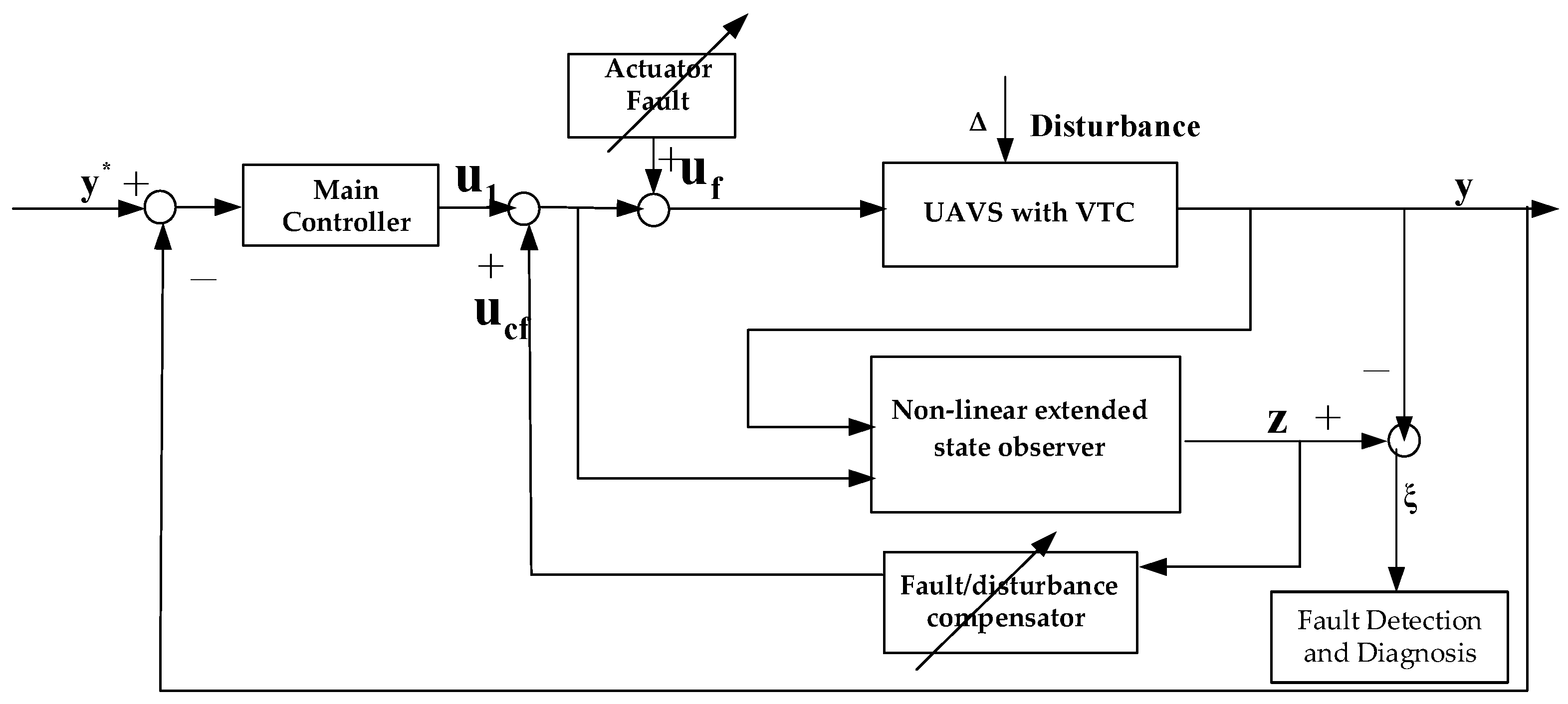
• A fault compensator designed by using the nonlinear extended state observer (NESO) technique. The NESO-based actuator fault/disturbance compensator can quickly estimate their impact and effectively compensate them, ensuring that the system is stable with degraded performance under fault conditions. In the faultless system, only the main controller is active. The compensator is automatically activated when an actuator fault or disturbance occurs.
• To verify the effectiveness of the method proposed in this paper, a UAV equipped with thrust vector control is chosen as the research object. The model is established for both normal and fault conditions. The main controller is designed using classical control theory, followed by the design of a fault compensation controller based on NESO theory. Simulations for different actuator faults confirm the effectiveness of controller.

The rest of the paper is organized as follows: Section 2 defines the problem and reviews relevant background knowledge, together with the formulation of the UAV under normal and actuator faults/disturbances. Section 3 describes the structure of the fault-tolerant controller based on the two-step approach, detailing the design of the main controller and the NESO-based fault compensator. Section 4 validates the proposed method through simulation results. Section 5 concludes the paper.

2. Problem Formulation and Preliminaries

We are considering commercial jet UAVs equipped with axisymmetric thrust vector nozzle, which are installed at the exhaust outlet of the UAV’s tail engine. Thrust vector nozzle can enhance control reconfiguration capabilities and reduce hardware redundancy of actuators. The goal is to develop a self-repairing transitional control law that enables the stability of flight control without waiting for fault detection and isolation results. Indeed, our method can be generalized to any control system with redundancy.

2.1. Dynamic Modeling of a UAV Equipped with Thrust Vectoring

During flight, aerodynamic control surfaces apply forces and moments to the UAV, thereby achieving attitude control and trajectory adjustment. When disturbances or actuator faults occur, these forces and moments change, leading to alterations of the UAV’s states. The first noticeable change is in the angular velocity, which is primarily controlled by the moments, followed by changes in other state variables influenced by aerodynamic forces. However, when comparing the moments and forces generated by aerodynamic control surfaces, the deflection of aerodynamic control surfaces primarily generates moments, whereas the forces they generate are relatively small. Therefore, the changes in the UAV’s state variables due to forces from a faulty actuator or disturbance can be considered negligible. If the angular velocity loop can be quickly stabilized during actuator failure, the UAV can maintain stability before the fault detection and diagnosis.

The angular velocity equation with aerodynamic moments and thrust-vectoring moments as inputs is as follows:

$$\left[\begin{array}{c}\dot{p}\\ \dot{q}\\ \dot{r}\end{array}\right]=h(x)+M\left[\begin{array}{c}l\\ m\\ n\end{array}\right]+M\left[\begin{array}{c}{l}_T\\ m_T\\ n_T\end{array}\right]$$

(1)

$$h(x)=\left[\begin{array}{c}-{\displaystyle \frac{I_{xz}(I_{yy}-I_{xx}-I_{zz})}{I_{xx}{I}_{zz}-I_{xz}^2}}pq-{\displaystyle \frac{{I_{zz}}^2-I_{zz}{I}_{yy}+{I_{xz}}^2}{I_{xx}{I}_{zz}-I_{xz}^2}}qr\\ {\displaystyle \frac{-pr(I_{xx}-I_{zz})-(p^2-r^2)I_{xz}) }{I_{yy}}}\\ -{\displaystyle \frac{I_{yy}{I}_{xx}-{I_{xx}}^2-{I_{xz}}^2}{I_{xx}{I}_{zz}-I_{xz}^2}}pq-{\displaystyle \frac{I_{xz}(I_{zz}-I_{yy}+I_{xx})}{I_{xx}{I}_{zz}-I_{xz}^2}}qr\end{array}\right]$$

(2)

$$M=\left[\begin{array}{ccc}{\displaystyle \frac{I_{zz}}{I_{xx}{I}_{zz}-I_{xz}^2}}& 0& {\displaystyle \frac{I_{xz}}{I_{xx}{I}_{zz}-I_{xz}^2}}\\ 0& {\displaystyle \frac{1}{I_{yy}}}& 0\\ {\displaystyle \frac{I_{xz}}{I_{xx}{I}_{zz}-I_{xz}^2}}& 0& {\displaystyle \frac{I_{xx}}{I_{xx}{I}_{zz}-I_{xz}^2}}\end{array}\right]$$

(3)

where p, q, and r are the roll angular velocity, pitch angular velocity, and yaw angular velocity; $\mathbf{M}$ is the inverse of moment of inertia matrix. l, m, and n are roll, pitch, and yaw aerodynamic moment provided by aerodynamic control surfaces; $l_T$, $m_T$, and $n_T$ are roll, pitch, and yaw moment provided by the thrust vector.

Considering the UAV equipped with a thrust vector nozzle, the nozzle simultaneously deflects up and down to generate lift and pitch moment while deflecting left and right to generate side force and yaw moment. The forces and moments generated by the thrust vector are as follows:

$$\left\{\begin{array}{l}{T}_x=T\cos ({\delta }_z)\cos ({\delta }_y)\approx T\\ T_y=T\cos ({\delta }_z)\sin ({\delta }_y)\approx T{\delta }_y\\ T_z=T\sin ({\delta }_z)\approx T{\delta }_z\end{array}\right.$$

(4)

$$\left\{\begin{array}{l}{l}_T=0\\ m_T=T_z{x}_T\\ n_T=-T_y{x}_T\end{array}\right.$$

(5)

where $T$ represents the thrust generated by thrust vectoring. $T_x$, $T_y$, and $T_z$ are the components of thrust along the coordinate axes. $x_T$ is the distance from the thrust application point to the center of gravity. ${\delta }_y$ and ${\delta }_z$ are the lateral and longitudinal deflection angles of the thrust nozzle. Since both ${\delta }_y$ and ${\delta }_z$ are small and lie between −15 degrees and 15 degrees, we can apply the approximation in Equation (4).

Therefore, Equation (1) can be rewritten as an affine nonlinear equation with aerodynamic control surfaces and thrust vectoring as inputs as follows:

$$\left[\begin{array}{c}\dot{p}\\ \dot{q}\\ \dot{r}\end{array}\right]=f(x)+g(x)u(t)+g_T(x)u_{cfT}(t)$$

(6)

$$f(x)=\left[\begin{array}{c}{f}_p(x)\\ f_q(x)\\ f_r(x)\end{array}\right]=\left[\begin{array}{c}{\displaystyle \frac{I_{zz}\cdot \widehat{l}}{I_{xx}{I}_{zz}-I_{xz}^2}}+{\displaystyle \frac{I_{xz}\cdot \widehat{n}}{I_{xx}{I}_{zz}-I_{xz}^2}}-{\displaystyle \frac{I_{xz}(I_{yy}-I_{xx}-I_{zz})}{I_{xx}{I}_{zz}-I_{xz}^2}}pq-{\displaystyle \frac{{I_{zz}}^2-I_{zz}{I}_{yy}+{I_{xz}}^2}{I_{xx}{I}_{zz}-I_{xz}^2}}qr\\ {I_{yy}}^{-1}(\widehat{m}-pr(I_{xx}-I_{zz})-(p^2-r^2)I_{xz}) \\ {\displaystyle \frac{I_{xz}\cdot \widehat{l}}{I_{xx}{I}_{zz}-I_{xz}^2}}+{\displaystyle \frac{I_{xx}\cdot \widehat{n}}{I_{xx}{I}_{zz}-I_{xz}^2}}-{\displaystyle \frac{I_{yy}{I}_{xx}-{I_{xx}}^2-{I_{xz}}^2}{I_{xx}{I}_{zz}-I_{xz}^2}}pq-{\displaystyle \frac{I_{xz}(I_{zz}-I_{yy}+I_{xx})}{I_{xx}{I}_{zz}-I_{xz}^2}}qr\end{array}\right]$$

(7)

where p, q, and r are roll angular velocity, pitch angular velocity, and yaw angular velocity. $\widehat{l}, \widehat{m}$, and $\widehat{n}$ represent the roll, pitch, and yaw aerodynamic moment when the aerodynamic control surface deflection is zero. $g(x)$ is the coefficient matrix of the known aerodynamic control surface inputs, and $u(t)={\left[\begin{array}{ccccc}{\delta }_{al}& {\delta }_{ar}& {\delta }_{el}& {\delta }_{er}& {\delta }_r\end{array}\right]}^T$ represents the control inputs of the five aerodynamic control surfaces, including the left and right ailerons, the left and right elevators, and the rudder.

$$\mathit{g}\left(\mathit{x}\right)=\left[\begin{array}{ccccc}{g}_{11}& g_{12}& g_{13}& g_{14}& g_{15}\\ g_{21}& g_{22}& g_{23}& g_{24}& g_{25}\\ g_{31}& g_{32}& g_{33}& g_{34}& g_{35}\end{array}\right]$$

(8)

In which,

$$\left[\begin{array}{c}{g}_{11}\\ g_{21}\\ g_{31}\end{array}\right]=\left[\begin{array}{l}{\displaystyle \frac{I_{zz}(QSb{C}_{l\delta al})+I_{xz}(QSb{C}_{n\delta al})}{I_{xx}{I}_{zz}-{I_{xz}}^2}}\\ {\displaystyle \frac{QSC{C}_{m\delta al}}{I_{yy}}}\\ {\displaystyle \frac{I_{xz}(QSb{C}_{l\delta al})+I_{xx}(QSb{C}_{n\delta al})}{I_{xx}{I}_{zz}-{I_{xz}}^2}}\end{array}\right],\left[\begin{array}{c}{g}_{12}\\ g_{22}\\ g_{32}\end{array}\right]=\left[\begin{array}{l}{\displaystyle \frac{I_{zz}(QSb{C}_{l\delta ar})+I_{xz}(QSb{C}_{n\delta ar})}{I_{xx}{I}_{zz}-{I_{xz}}^2}}\\ {\displaystyle \frac{QSC{C}_{m\delta ar}}{I_{yy}}}\\ {\displaystyle \frac{I_{xz}(QSb{C}_{l\delta ar})+I_{xx}(QSb{C}_{n\delta ar})}{I_{xx}{I}_{zz}-{I_{xz}}^2}}\end{array}\right]$$

$$\left[\begin{array}{c}{g}_{13}\\ g_{23}\\ g_{33}\end{array}\right]=\left[\begin{array}{l}{\displaystyle \frac{I_{zz}(QSb{C}_{l\delta el})+I_{xz}(QSb{C}_{n\delta el})}{I_{xx}{I}_{zz}-{I_{xz}}^2}}\\ {\displaystyle \frac{QSC{C}_{m\delta el}}{I_{yy}}}\\ {\displaystyle \frac{I_{xz}(QSb{C}_{l\delta el})+I_{xx}(QSb{C}_{n\delta el})}{I_{xx}{I}_{zz}-{I_{xz}}^2}}\end{array}\right],\left[\begin{array}{c}{g}_{14}\\ g_{24}\\ g_{34}\end{array}\right]=\left[\begin{array}{l}{\displaystyle \frac{I_{zz}(QSb{C}_{l\delta er})+I_{xz}(QSb{C}_{n\delta er})}{I_{xx}{I}_{zz}-{I_{xz}}^2}}\\ {\displaystyle \frac{QSC{C}_{m\delta er}}{I_{yy}}}\\ {\displaystyle \frac{I_{xz}(QSb{C}_{l\delta er})+I_{xx}(QSb{C}_{n\delta er})}{I_{xx}{I}_{zz}-{I_{xz}}^2}}\end{array}\right]$$

$$\left[\begin{array}{c}{g}_{15}\\ g_{25}\\ g_{35}\end{array}\right]=\left[\begin{array}{l}{\displaystyle \frac{I_{zz}(QSb{C}_{l\delta r})+I_{xz}(QSb{C}_{n\delta r})}{I_{xx}{I}_{zz}-{I_{xz}}^2}}\\ 0\\ {\displaystyle \frac{I_{xz}(QSb{C}_{l\delta r})+I_{xx}(QSb{C}_{n\delta r})}{I_{xx}{I}_{zz}-{I_{xz}}^2}}\end{array}\right]$$

where $Q={\displaystyle \frac{1}{2}}\rho V^2$ is the dynamic pressure, $\rho$ is the air density, $V$ is the velocity of the UAV, $S$ is the wing area, $C$ is the aerodynamic chord, and $b$ is the wingspan length. $C_{l{\delta }_i}, C_{m{\delta }_i}, {\mathrm{and} C}_{n{\delta }_i}$ represent the roll moment coefficient, pitch moment coefficient, and yaw moment coefficient corresponding to each control surface respectively.

$u_{cfT}={\left[\begin{array}{cc}{\delta }_z& {\delta }_y\end{array}\right]}^T$ represents the control inputs for thrust vectoring, and $g_T(x)$ is the coefficient matrix for the thrust-vectoring control inputs. Assume that thrust vectoring only generates pitch and yaw moments.

$$g_T(x)=M*\left[\begin{array}{cc}0& 0\\ T{x}_T& 0\\ 0& -T{x}_T\end{array}\right]$$

(9)

The aerodynamic control surfaces can generate roll, pitch, and yaw moments, while the thrust vectoring can also generate pitch and yaw moments. These mechanisms control the UAV’s rotational motion in three degrees of freedom, offering redundancy in control inputs. Under normal conditions, a direct allocation strategy assumes the UAV is controlled solely by aerodynamic control surfaces, without activating thrust vectoring. In cases of actuator failure or disturbances, the thrust vectoring is activated to ensure the UAV’s stable flight.

On the other hand, since the thrust vectoring studied in this paper cannot generate roll moments, actuator faults generally affect moments in all three directions. If the impact of the fault/disturbance on the roll moment is not compensated in time, the UAV’s lateral and directional motion will quickly diverge, which will directly lead to the instability of the entire flight control system. UAV’s ailerons can provide larger roll moments comparing to the elevator and rudder. Therefore, in this paper, aileron failure is not considered. Instead, additional aileron signals are used in cooperation with thrust vectoring to compensate for changes in three-axis moments caused by failures or disturbances.

Therefore, Equation (1) can be rewritten as follows:

$$\left[\begin{array}{c}\dot{p}\\ \dot{q}\\ \dot{r}\end{array}\right]=f(x)+g(x)u(t)+g_c(x)u_{cf}(t)$$

(10)

where redundant control input $u_{cf}={\left[\begin{array}{ccc}\Delta {\delta }_a& {\delta }_z& {\delta }_y\end{array}\right]}^T$, which represents the additional aileron deflection signals and thrust-vectoring deflection signals. $g_c(x)$ is the input coefficient matrix for the redundant control surfaces.

$$g_c(x)=M\times \left[\begin{array}{ccc}QSb{C}_{l{\delta }_a}& 0& 0\\ 0& T{x}_T& 0\\ QSb{C}_{n{\delta }_a}& 0& -T{x}_T\end{array}\right]$$

(11)

Under normal conditions, the redundant control input $u_{cf}$ remains zero and is only activated under the fault/disturbance.

2.2. Modeling of Aircraft with Actuator Faults and Disturbance

For the flight control system, the angular velocity loop equation considering actuator faults and disturbance can be written as follows:

$$\left[\begin{array}{c}\dot{p}\\ \dot{q}\\ \dot{r}\end{array}\right]=f\left(x\right)+g\left(x\right)u_1\left(t\right)+g\left(x\right)u_f\left(t\right)+\Delta \left(x,u_1,t\right)+g_c(x)u_{cf}(t)$$

(12)

where $u_1\left(t\right)\in R^m$ represents the desired actuator command signal provided by the controller that is designed for high performance and a certain level of robustness. $u_f={\left[\begin{array}{ccccc}{\delta }_{alf}& {\delta }_{arf}& {\delta }_{elf}& {\delta }_{erf}& {\delta }_{rf}\end{array}\right]}^T$ represents the actuator failure, and $\Delta \left(x,u,t\right)$ represents the disturbances and system’s uncertainty.

The following describes the expressions of $u_f(t)$ under three common actuator faults.

• Stuck or Jammed Failure: Assuming the $i-\mathrm{th}$ control surface is jammed at an angle of $x$, then $u_f(t)={[0,\dots ,x-u_{1i}(t),\dots ,0]}^T$.
• Partial Damage Failure: Assuming the $i-\mathrm{th}$ control surface, such as the left elevator, is damaged by $x$ percent, then $u_f(t)={[0,\dots ,(x-1)u_{1i}(t),\dots ,0]}^T$.
• Complete Failure: Assuming the $i-\mathrm{th}$ control surface is fluctuating, then $u_f(t)={[0,\dots ,-u_{1i}(t),\dots ,0]}^T$.

By comparing Equations (5) and (7) using the expressions of $u_f(t)$ under different fault conditions, it follows that $u(t)=u_1\left(t\right)+u_f\left(t\right)$.

3. Two-Step Fault-Tolerant Controller Design

3.1. Fault-Tolerant Controller Structure

A robust fault-tolerant controller structure is proposed for linear system [38]. We extend it to nonlinear flight control systems, with the structure shown as follows:

In Figure 1, ${\mathit{y}}^{*}$ represents the given reference signal, $u_1$ represents the output signal of the main controller, which is designed for high performance and a certain level of robustness, $u_f$ and $\Delta$ are the actuator faults and disturbances, which can be considered as the additional input, $u_{cf}$ is the compensator input, $\mathit{y}$ is the system outputs, $z$ is the output of the nonlinear system observer, and $\mathit{\xi }=z-y$ is the residual signal, which can be used for fault detection and diagnosis.

In this structure, the main controller and the compensation controller can be designed independently. When the system is faultless, indicating $u_f=0$, $\mathbf{\xi }$ are approximately zero, and the compensation controller $u_{cf}$ is also approximately zero, meaning that thrust-vectoring and additional aileron deflection are not activated, and only the main controller $u_1$ is active. When the actuator fault or disturbance occurs, the compensation controller is automatically activated, and it mainly ensures the stability of the system and compensates the impact of the fault/disturbance. Normally, system performance will experience significant degradation under faults or disturbances, even with the compensator added.

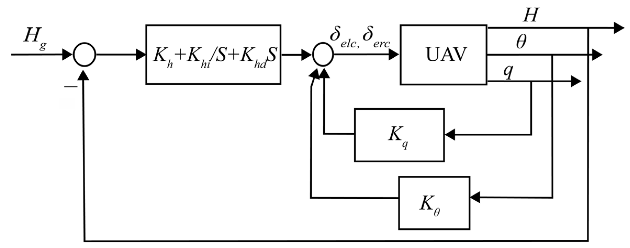
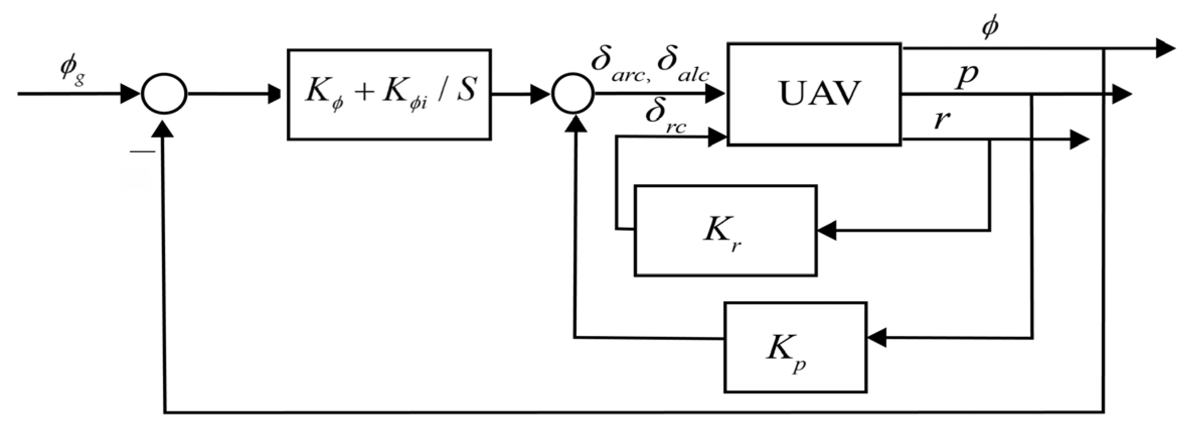
3.2. Main Controller Design

The main controller can be designed using any existing control theories, focusing primarily on the system’s performance. Although there are currently very advanced flight control technologies such as adaptive control, dynamic inversion control, and neural network control to demonstrate the effectiveness of the control structure proposed in this paper, we use the traditional PID method to design the main controller.

The formulas for the position and attitude angles are as follows:

$$\left\{\begin{array}{l}\dot{x}=V\cos \gamma \cos \chi \\ \dot{y}=V\cos \gamma \sin \chi \\ \dot{H}=V\sin \gamma \end{array}\right.$$

(13)

where $x \mathrm{and} y$ represent the position of the UAV along the x-axis and y-axis relative to the ground, $H$ represents altitude, $\chi$ represents track azimuth angle, and $\gamma$ represents track slope angle.

$$\left\{\begin{array}{l}\dot{\varphi }=p+(q\sin \varphi +r\cos \varphi )\tan \theta \\ \dot{\theta }=q\cos \varphi -r\sin \varphi \\ \dot{\psi }=(q\sin \varphi +r\cos \varphi )/\cos \theta \end{array}\right.$$

(14)

where $\varphi ,\theta , \mathrm{and}\psi$ represent roll angle, pitch angle, and yaw angle.

For the UAV, the longitudinal and lateral-directional dynamics are nearly fully decoupled, making it suitable to apply the classical root locus method for designing the autopilot control laws.

The longitudinal control system of a UAV primarily controls the pitch angle, altitude, and speed. Based on the different time-varying variables, the flight control system adopts a control strategy of inner-loop followed by outer-loop control.

A typical PID control law is designed for the UAV’s altitude as follows and the control structure is shown in Figure 2:

$${\delta }_{elc}={\delta }_{erc}=K_{q}q+K_{\theta }\theta +K_{hd}\mathrm{\Delta }\dot{H}+K_h\Delta H+K_{hi}{\displaystyle \int \Delta H}$$

(15)

where ${\delta }_{elc}$ and ${\delta }_{erc}$ are the deflection angles of the left and right elevators, $q$ is the pitch rate, $\theta$ is the pitch angle, $\Delta H=H-H_g$ is the altitude difference relative to the reference altitude $H_g$, and $K_q$, $K_{\theta }$, $K_{hd}$, $K_h$, and $K_{hi}$ are the proportional gains.

Similarly for the lateral-directional control system, the PID control law for the roll angle is as follows and the control structure is shown in Figure 3:

$$\begin{array}{l}{\delta }_{arc}=-{\delta }_{alc}=K_{p}p+K_{\varphi }\Delta \varphi +K_{\varphi i}{\displaystyle \int \Delta \varphi }\\ {\delta }_{rc}=K_{r}r\end{array}$$

(16)

where ${\delta }_{arc}$, ${\delta }_{alc}$, and ${\delta }_{rc}$ are the deflection angles of the left and right aileron and rudder, $\Delta \varphi =\varphi -{\varphi }_g$ is the roll angle difference relative to the reference altitude ${\varphi }_g$, and $K_p$, $K_{\varphi }$, $K_{\varphi i}$, and $K_r$ are the proportional gains.

3.3. Fault Estimation Based on Nonlinear Extended State Observer

In Equation (12), we know that the function including actuator fault and disturbance can be expressed as follows:

$$F(x,t)=g\left(x\right)u_f\left(t\right)+\Delta \left(x,u_1,t\right)$$

(17)

Equation (12) can be rewritten as follows:

$$\left[\begin{array}{c}\dot{p}\\ \dot{q}\\ \dot{r}\end{array}\right]=f\left(x\right)+g\left(x\right)u_1\left(t\right)+F(x,t)+g_c(x)u_{cf}(t)$$

(18)

if we find a solution that can estimate this $F(x,t)$, then let

$$g_c(x)u_{cf}(t)=-F(x,t)$$

(19)

If the right inverse matrix of $g_c(x)$ exists, we can easily obtain

$$u_{cf}(t)=-g_c^{-1}(x)F(x,t)$$

(20)

NESO is a nonlinear observer designed for affine nonlinear systems. The basic idea of NESO is to view the system disturbances and faults as an extended state of the system and then estimate the state and the extended state simultaneously. This paper estimates the faults together with disturbances for multi-input, multi-output nonlinear systems based on three NESOs.

We apply the NESO theory based on the UAV model proposed in Section 2. The UAV model with actuator faults and disturbances without redundant control input is as follows:

$$\begin{array}{cc}\left[\begin{array}{c}\dot{p}\\ \dot{q}\\ \dot{r}\end{array}\right]& =f\left(x\right)+g\left(x\right)u_1\left(t\right)+g(x)u_f(t)+\Delta (x,u_1,t)\\ & =\left[\begin{array}{c}{f}_1(x)\\ f_2(x)\\ f_3(x)\end{array}\right]+\left[\begin{array}{c}{U}_1(x,u_1,t)\\ U_2(x,u_1,t)\\ U_3(x,u_1,t)\end{array}\right]+\left[\begin{array}{c}{F}_1(x,u_f,t)\\ F_2(x,u_f,t)\\ F_3(x,u_f,t)\end{array}\right]\end{array}$$

(21)

$F_i(x,u_f)$ represents the unknown fault function, where $F_i=g_{ij}{u}_f+\Delta$ and $i\in 1,2,3; j\in 1,2,3,4,5$. When an actuator fault or disturbance happens, we can use three NESOs to estimate $F_1(x,u_f)$, $F_2(x,u_f)$, and $F_3(x,u_f)$ corresponding to roll, pitch, and yaw angle rate fault function.

Taking the roll channel as an example, we assume the system experiences a left elevator jam fault. According to the NESO, the extended state $x_{2p}=F_1(x,u_f)$ is selected, and it is assumed that ${\dot{x}}_{2p}(t)=v(t)$. Thus, the roll channel equation is expressed as follows:

$$\left\{\begin{array}{l}\dot{p}=f_1+U_1+F_1\\ {\dot{x}}_{2p}(t)=v(t)\\ y=p\end{array}\right.$$

(22)

The corresponding extended state observer is given as follows:

$$\left\{\begin{array}{l}{e}_p=z_p-p\\ {\dot{z}}_p=z_{2p}+f_1+U_1-{\beta }_1{g}_1(e_p)\\ {\dot{z}}_{2p}=-{\beta }_2{g}_2(e_p)\end{array}\right.$$

(23)

in which,

$$\begin{array}{l}{g}_1(e_p)=e_p\\ g_2(e_p)=fal(e_p,{\displaystyle \frac{1}{2}},\delta )=\left\{\begin{array}{l}{\left|e_p\right|}^{\alpha }sign(e_p)\hspace{1em} \left|e_p\right|>\delta \\ e_p/{\delta }^{1-\alpha }\hspace{1em}\hspace{1em}\hspace{1em}\left|e_p\right|\le \delta \end{array}\right.\end{array}$$

By selecting appropriate parameters ${\beta }_1$, ${\beta }_2$, and $\delta$, the convergence $z_p\to p$ and $z_{2p}\to F_1$ can be achieved. Similarly, extended state observers can be established for the pitch and yaw channels to obtain the fault function estimates $z_{2q}\to F_2$ and $z_{2r}\to F_3$, respectively.

3.4. Fault Compensator Design

By using three separate NESOs to estimate the fault and disturbance functions, the following results can be obtained:

$$\left[\begin{array}{l}{z}_{2p}\\ z_{2q}\\ z_{2r}\end{array}\right]=\left[\begin{array}{c}{F}_1(x,u_f,t)\\ F_2(x,u_f,t)\\ F_3(x,u_f,t)\end{array}\right]=g(x)u_f(t)+\Delta (x,u_1,t)$$

(24)

Therefore, the compensation control law is obtained form (20) as follows:

$$u_{cf}=-g_c^{-1}\left[\begin{array}{l}{z}_{2p}\\ z_{2q}\\ z_{2r}\end{array}\right]$$

(25)

Note that in this paper, since $g_c$ is a square matrix, the compensation control input $u_{cf}$ is unique. However, if the UAV has more control redundancy, i.e., $g_c\in R^{n*m}(m>n)$, control allocation should be performed based on the compensation moment by the redundant control surfaces.

3.5. Closed-Loop Stability

For any fault-tolerant control system, the stability of the closed-loop system is crucial. In this paper, the entire closed-loop system with compensator based on NESO is as follows:

$$\left\{\begin{array}{l}\dot{x}=f\left(x\right)+g\left(x\right)u_1\left(t\right)+g(x)u_f(t)+\Delta (x,t)+g_c(x)u_{cf}(t)\\ {\dot{e}}_1=e_2-{\beta }_1{g}_1(e_1)\\ {\dot{e}}_2=-{\beta }_2{g}_2(e_1)-v(t)\end{array}\right.$$

(26)

where ${\mathrm{e}}_1=\left[\begin{array}{c}{\mathrm{z}}_{\mathrm{p}}\\ {\mathrm{z}}_{\mathrm{q}}\\ {\mathrm{z}}_{\mathrm{r}}\end{array}\right]-\left[\begin{array}{c}\mathrm{p}\\ \mathrm{q}\\ \mathrm{r}\end{array}\right]$ represents the states estimation errors, and ${\mathrm{e}}_2=\left[\begin{array}{c}{\mathrm{z}}_{2\mathrm{p}}\\ {\mathrm{z}}_{2\mathrm{q}}\\ {\mathrm{z}}_{2\mathrm{r}}\end{array}\right]-\left[\begin{array}{c}{\mathrm{x}}_{2\mathrm{p}}\\ {\mathrm{x}}_{2\mathrm{q}}\\ {\mathrm{x}}_{2\mathrm{r}}\end{array}\right]$ represents the extended state estimation errors. The definitions of ${\mathsf{\beta }}_{\mathbf{1}}$, ${\mathsf{\beta }}_{\mathbf{2}}$, ${\mathbf{g}}_{\mathbf{1}}\left({\mathbf{e}}_{\mathbf{1}}\right)$, ${\mathbf{g}}_{\mathbf{2}}\left({\mathbf{e}}_{\mathbf{1}}\right)$, and $\mathbf{v}\left(\mathbf{t}\right)$ are the same as in Equations (22) and (23).

By substituting Equation (25) into Equation (26), we can obtain the following:

$$\begin{array}{l}\dot{x}=f\left(x\right)+g\left(x\right)u_1(t)+g(x)u_f(t)+\Delta (x,t)+g_c(x)*(-{g_c}^{-1}(x)\left[\begin{array}{l}{z}_{2p}\\ z_{2q}\\ z_{2r}\end{array}\right])\\ =f\left(x\right)+g\left(x\right)u_1(t)+\xi \end{array}$$

(27)

where $\mathsf{\xi }=\mathbf{g}(\mathbf{x}){\mathbf{u}}_{\mathbf{f}}\left(\mathrm{t}\right)+\mathsf{\Delta }(\mathbf{x},\mathrm{t}) -\left[\begin{array}{c}{\mathrm{z}}_{2\mathrm{p}}\\ {\mathrm{z}}_{2\mathrm{q}}\\ {\mathrm{z}}_{2\mathrm{r}}\end{array}\right]$.

According to the compensator based on NESO, we know that by selecting appropriate parameters ${\mathsf{\beta }}_{\mathbf{1}} \mathrm{a}\mathrm{n}\mathrm{d} {\mathsf{\beta }}_{\mathbf{2}}$, it is possible to make

$$\left[\begin{array}{l}{z}_{2p}\\ z_{2q}\\ z_{2r}\end{array}\right]\to g(x)u_f(t)+\Delta (x,t)$$

(28)

then $\mathsf{\xi }\to 0$ can be obtained. So, we can give Assumption 1.

Assumption 1

([39]). For the system as shown below in Equation (27), there exists a main controller $u_1\left(t\right)=\beta \left(x\right)$, such that the closed-loop system in Equation (27) is exponentially asymptotically stable.

According to Assumption 1, the closed-loop system is exponentially asymptotically stable under the control law $\beta \left(x\right)$, which means there exists a continuously differentiable Lyapunov function $V_1 > 0$ that satisfies the inequality:

$${\dot{V}}_1={\displaystyle \frac{\partial V_1}{\partial x}}[f(x)+g(x)\beta (x)+\xi ]<-\gamma ‖x‖<0$$

(29)

where $\gamma$ is a small positive number.

Lemma 1

([39]). Define a Lyapunov function $V_2$ for $\left\{\begin{array}{c}{\dot{\mathbf{e}}}_{\mathbf{1}}={\mathbf{e}}_{\mathbf{2}}-{\mathbf{\beta }}_{\mathbf{1}}{\mathbf{g}}_{\mathbf{1}}\left({\mathbf{e}}_{\mathbf{1}}\right)\\ {\dot{\mathbf{e}}}_{\mathbf{2}}=-{\mathbf{\beta }}_{\mathbf{2}}{\mathbf{g}}_{\mathbf{2}}\left({\mathbf{e}}_{\mathbf{1}}\right)-\mathbf{v}\left(\mathbf{t}\right)\end{array}\right.$,

$$V_2={\displaystyle \frac{1}{2}}{H}^2(e_1,e_2)$$

(30)

where

$$H(e_1,e_2)=\left\{\begin{array}{l}\left|h_1(e_1,e_2)\right|, \mathrm{if} \left|h_1(e_1,e_2)\right|>h_2(e_1)\\ h_2(e_1), \hspace{1em} \mathrm{otherwise}\end{array}\right.$$

(31)

$$h_1(e_1,e_2)=e_2-{\beta }_1{g}_1(e_1)+k{h}_2(e_1)sign(e_1),k>1$$

(32)

$$h_2(e_1)={\displaystyle \frac{{\beta }_2}{k{\beta }_1}}\left|g_2(e_1)\right|$$

(33)

If the parameters ${\mathsf{\beta }}_1 \mathrm{and} {\mathsf{\beta }}_2$ are selected appropriately to ensure the condition ${\mathsf{\beta }}_1^2 > 4\mathrm{k}{\mathsf{\beta }}_2\left|{\displaystyle \frac{\mathbf{d}{\mathbf{g}}_2\left({\mathbf{e}}_1\right)}{\mathbf{d}{\mathbf{e}}_1}}\right|$ are satisfied, then ${\dot{V}}_2 < 0$.

Lemma 2

([39]). Defines a Lyapunov function as follows for closed-loop system in Equation (26).

$$V=V_1+V_2>0$$

(34)

If Assumption 1 and Lemma 1 are satisfied, then $\dot{V}={\dot{V}}_1+{\dot{V}}_2 < 0$, the entire closed-loop system in Equation (26) is stable.

4. Simulation Results and Discussion

In this section, we present the results of our simulations to verify the effectiveness of the method presented in this paper. The initial conditions for the simulation are as follows: the flight speed is $264 \mathrm{m}/\mathrm{s}$, and the altitude is $5000 \mathrm{m}$, with the aircraft in a level flight state.

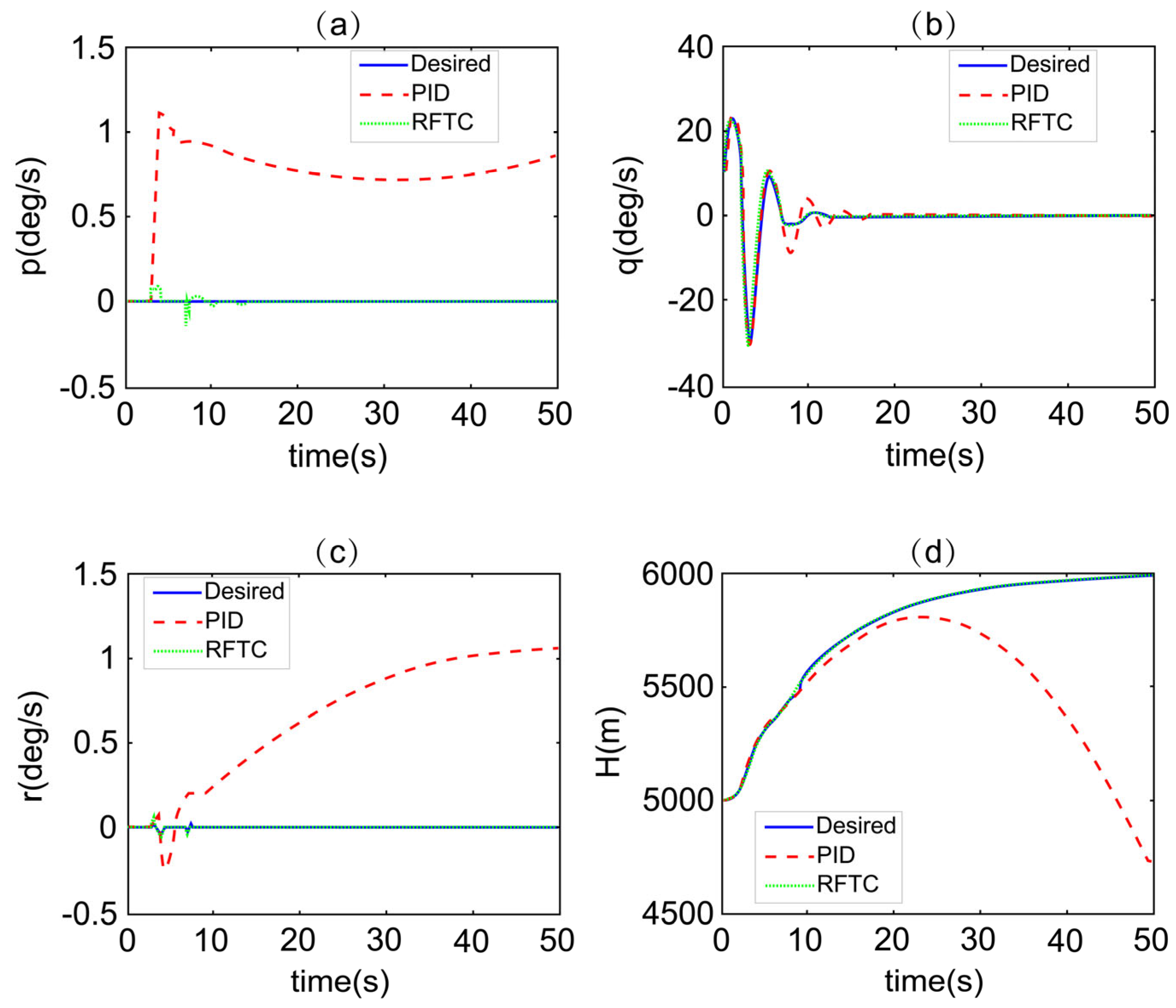
4.1. Case 1: Elevator Fault

During the climbing flight of the UAV at a reference altitude signals $H_g=6000 \mathrm{m}$, the main controller is designed based on Equation (8).

At 3 s, the left elevator gets stuck at its maximum limit of 30 degrees. The simulation results are shown in Figure 4.

Under normal conditions, the UAV’s state responses are shown by the blue solid lines in Figure 4. The UAV demonstrates desired climb performance, smoothly ascending to an altitude of 6000 m.

At 3 s, the left elevator gets stuck at 30 degrees, which is the most severe type of control surface jam failure. The UAV’s response is shown by the red dashed lines in Figure 4 relying only on the PID controller. Due to the fault, the aircraft experiences lateral-directional motion, the roll angular velocity in Figure 4a, and yaw angular velocity in Figure 4c diverges within a short period. At the same time, the flight altitude begins to rapidly decrease, indicating that the aircraft’s longitudinal motion becomes unstable. This shows that under severe failure conditions, if no compensation is added, the primary control alone is insufficient to ensure the stability of the system.

The green dotted lines in Figure 4 represent the aircraft’s responses with the fault compensator employing thrust vectoring and ailerons. After compensation, the oscillations in altitude and angular velocity caused by the failure are suppressed after a short period. The three-axis angular velocity responses and altitude response are almost entirely consistent with the fault-free state responses.

Figure 5 illustrates the fault function estimated by the NESO observer, which models the fault function as an extended state, with the extended state values being nearly zero before 3 s; after the fault happens, the extended state values exhibit a sudden change. It is evident from Figure 5 that the fault occurs at 3 s. The generated extended state values represent the fault estimation value.

$$g(x)u_f(t)+\Delta (x,u_1,t)={\left[\begin{array}{ccc}{F}_1& F_2& F_3\end{array}\right]}^T={[z_{2p},z_{2q},z_{2r}]}^T$$

(35)

where $u_f\left(t\right)={\left[0& \hspace{1em}0& \hspace{1em}30/57.3-{\delta }_{elc}& \hspace{1em}0& \hspace{1em}0\right]}^T$.

Figure 6 illustrates the deflection of control surfaces under the proposed robust fault-tolerant controller. During the initial 3 s of climbing, only the elevator is deflected, while the aileron, rudder, and thrust vectoring remain inactive. After 3 s, the left elevator gets stuck at 30 degrees, producing positive rolling moments, positive yawing moments, and negative pitching moments. By using the compensator, the aileron deflects to generate negative rolling moments, negative yawing moments simultaneously. The yawing moments generated by the ailerons can completely counteract the yaw motion caused by the fault, eliminating the need for the thrust-vectoring system to provide additional yawing moments. Meanwhile, to maintain the aircraft at an altitude of 6000 m, the thrust-vectoring system generates positive pitching moments to raise the aircraft’s nose, counteracting the nose-down pitching moment caused by the fault in the left elevator.

4.2. Case 2: Rudder Fault

The second scenario involved tracking reference roll angle signal, which are given by the following equation: ${\phi }_g={15}^0$. The main controller is designed based on Equation (9).

Under normal conditions, the solid lines in Figure 7 show that the UAV maintains altitude-holding circular flight under the PID control law. The UAV demonstrates excellent tracking performance. At 1 s, the rudder jams at 7 degrees. The dashed lines show the UAV’s state responses under the PID controller alone without the fault compensator. It can be observed that the lateral-directional response especially in Figure 7e rapidly deteriorates, and the UAV becomes unstable within a short period. The dotted lines in Figure 7 represent the aircraft’s response after timely adding the fault compensator. It can be seen that the roll angle in Figure 7e stabilizes around 10 degrees. Compared to faultless conditions, the system’s tracking performance is slightly reduced. However, the system remains stable, achieving the goal of robust control.

Figure 8 illustrates the fault function estimated by the NESO observer. The extended state values are nearly zero before 1 s; after the fault happens, the extended state values exhibit a sudden change. The generated extended state values represent the fault estimation value as follows:

$$g(x)u_f(t)+\Delta (x,u_1,t)={\left[\begin{array}{ccc}{F}_1& F_2& F_3\end{array}\right]}^T={[z_{2p},z_{2q},z_{2r}]}^T$$

(36)

In which, $u_f\left(t\right)={\left[0& \hspace{1em}0& \hspace{1em}0& \hspace{1em}0& \hspace{1em}7/57.3-{\delta }_{rc}\right]}^T$.

When the rudder is stuck at 7 degrees, positive roll moments and negative yaw moments are generated. The ailerons should deflect positively to generate negative roll moments to counteract the positive roll moments caused by the rudder fault, but the positive deflection of the ailerons will create negative yaw moments, which is unsuitable for compensating the yaw moment. If the thrust-vectoring system can simultaneously neutralize the effects of both the fault-induced yaw moment and the yaw moment caused by additional aileron signals, the system can return to a fault-free state. However, if the fault is too severe and the thrust-vectoring system cannot fully counteract the yaw moment’s impact on the aircraft, flight quality will be significantly affected. As shown in Figure 9, the thrust-vectoring deflection ${\delta }_y$ reaches its limit, yet the system state has not returned to a fault-free condition. This indicates that, in this flight state, due to the limited capability of the thrust-vectoring system, the yaw moment generated is insufficient to fully counteract the rudder fault and the additional yaw moment induced by the ailerons. Although complete fault compensation is not achieved, the thrust vectoring effectively suppresses aircraft state divergence and ensures system stability. Furthermore, since the rudder fault has almost no effect on the pitch moment, the thrust vector deflection angle ${\delta }_z=0$ degrees.

The simulation results in this section show that for UAVs with thrust vectoring, the designed two-step robust fault-tolerant control law exhibits good robustness to certain degrees of elevator and rudder failures.

5. Conclusions

We propose a robust fault-tolerant controller structure to address UAV actuator faults and disturbances, which is implemented by using a two-step method. The main controller is focused on system performance and adaptable to various existing control theories, while the fault compensator is designed based on fault estimation using NESO. This controller can balance system performance, robustness, and fault tolerance. Simulation results demonstrate that the controller can act as an emergency transitional control law for a self-repairing flight control system while also providing a foundation for precise fault detection and diagnosis in subsequent stages. This method is only applicable to UAVs with control redundancy. Future research should focus on experimental validation, addressing more faults, and exploring control reconfiguration strategies to further enhance the robustness and applicability of the control framework.

References

1. Doornbos, J.; Bennin, K.E.; Babur, Ö.; Valente, J. Drone Technologies: A Tertiary Systematic Literature Review on a Decade of Improvements. IEEE Access 2024, 12, 23220–23239. [Google Scholar] [CrossRef]
2. Tsouros, D.C.; Bibi, S.; Sarigiannidis, P.G. A Review on UAV-Based Applications for Precision Agriculture. Information 2019, 10, 349. [Google Scholar] [CrossRef]
3. Mohsan, S.A.H.; Khan, M.A.; Noor, F.; Ullah, I.; Alsharif, M.H. Towards the Unmanned Aerial Vehicles (UAVs): A Comprehensive Review. Drones 2022, 6, 147. [Google Scholar] [CrossRef]
4. Zhang, A.; Xu, H.; Bi, W.; Xu, S. Adaptive Mutant Particle Swarm Optimization Based Precise Cargo Airdrop of Unmanned Aerial Vehicles. Appl. Soft Comput. 2022, 130, 109657. [Google Scholar] [CrossRef]
5. Xing, L.; Johnson, B.W. Reliability Theory and Practice for Unmanned Aerial Vehicles. IEEE Internet Things J. 2023, 10, 3548–3566. [Google Scholar] [CrossRef]
6. Hou, D.; Su, Q.; Song, Y.; Yin, Y. Research on Drone Fault Detection Based on Failure Mode Databases. Drones 2023, 7, 486. [Google Scholar] [CrossRef]
7. Zolghadri, A. A Review of Fault Management Issues in Aircraft Systems: Current Status and Future Directions. Prog. Aerosp. Sci. 2024, 147, 101008. [Google Scholar] [CrossRef]
8. Raja, M.S.K.; Ali, Q. Recent Advances in Active Fault-Tolerant Flight Control Systems. Proc. Inst. Mech. Eng. Part G J. Aerosp. Eng. 2022, 236, 2151–2161. [Google Scholar] [CrossRef]
9. Wu, Q.; Zhu, Q. Prescribed Performance Fault-Tolerant Attitude Tracking Control for UAV with Actuator Faults. Drones 2024, 8, 204. [Google Scholar] [CrossRef]
10. Amin, A.A.; Hasan, K.M. A Review of Fault Tolerant Control Systems: Advancements and Applications. Measurement 2019, 143, 58–68. [Google Scholar] [CrossRef]
11. Fekih, A. Fault Tolerant Control Design for Complex Systems: Current Advances and Open Research Problems. In Proceedings of the 2015 IEEE International Conference on Industrial Technology (ICIT), Seville, Spain, 17–19 March 2015; pp. 1007–1012. [Google Scholar] [CrossRef]
12. Jiang, J.; Yu, X. Fault-Tolerant Control Systems: A Comparative Study Between Active and Passive Approaches. Annu. Rev. Control 2012, 36, 60–72. [Google Scholar] [CrossRef]
13. Estrada, M.A.; Fridman, L.; Moreno, J.A. Passive Fault-Tolerant Control via Sliding-Mode-Based Lyapunov Redesign. IEEE Trans. Autom. Control 2024, 69, 6777–6788. [Google Scholar] [CrossRef]
14. Srour, A.; Noura, H.; Theilliol, D. Passive Fault-Tolerant Control of a Fixed-Wing UAV Based on Model-Free Control. In Proceedings of the 5th International Conference on Control and Fault-Tolerant Systems (SysTol), Saint-Raphael, France, 29 September–1 October 2021; pp. 109–114. [Google Scholar] [CrossRef]
15. Wei, Y.; Sheng, L.; Gao, M.; Ma, Y. Anti-Saturation Fault-Tolerant Control for Markov Jump Nonlinear Systems with Unknown Control Coefficients and Unmodeled Dynamics. Nonlinear Anal. Hybrid Syst. 2023, 50, 101384. [Google Scholar] [CrossRef]
16. Ma, Y.; Gao, M.; Sheng, L.; Wei, Y. Active Fault Tolerant Control for Polynomial Nonlinear Systems with Asymmetric State Constraints and Measurement Noise. Nonlinear Dyn. 2023, 111, 14157–14175. [Google Scholar] [CrossRef]
17. Shen, Q.; Yue, C.; Goh, C.H.; Wang, D. Active Fault-Tolerant Control System Design for Spacecraft Attitude Maneuvers with Actuator Saturation and Faults. IEEE Trans. Ind. Electron. 2019, 66, 3763–3772. [Google Scholar] [CrossRef]
18. Cheng, X.; Gao, M.; Sheng, L.; Wei, Y. Fixed-Time Active Fault-Tolerant Control for a Class of Nonlinear Systems with Intermittent Faults and Input Saturation. J. Process Control 2024, 143, 103319. [Google Scholar] [CrossRef]
19. Fan, Z.; Wang, L.; Meng, H.; Yang, C. Data-Based Deep Reinforcement Learning and Active FTC for Unmanned Surface Vehicles. J. Frankl. Inst. 2024, 361, 106960. [Google Scholar] [CrossRef]
20. Cheng, X.; Gao, M.; Huai, W.; Niu, Y.; Sheng, L. Fixed-Time Active Fault-Tolerant Control for Dynamical Systems with Intermittent Faults and Unknown Disturbances. Appl. Math. Comput. 2025, 486, 129054. [Google Scholar] [CrossRef]
21. Mazare, M.; Taghizadeh, M.; Ghaf-Ghanbari, P.; Davoodi, E. Robust Fault Detection and Adaptive Fixed-Time Fault-Tolerant Control for Quadrotor UAVs. Robot. Auton. Syst. 2024, 179, 104747. [Google Scholar] [CrossRef]
22. Liu, S.; Zheng, Z.; Zhu, B.; Guan, Z. Adaptive Fault-Tolerant Control for Attitude Tracking of a Carrier-Based Aircraft Subject to Actuator Faults. IEEE Trans. Aerosp. Electron. Syst. 2024, 60, 6133–6145. [Google Scholar] [CrossRef]
23. Wang, B.; Zhu, D.; Han, L.; Gao, H.; Gao, Z.; Zhang, Y. Adaptive Fault-Tolerant Control of a Hybrid Canard Rotor/Wing UAV Under Transition Flight Subject to Actuator Faults and Model Uncertainties. IEEE Trans. Aerosp. Electron. Syst. 2023, 59, 4559–4574. [Google Scholar] [CrossRef]
24. Chen, Y.; Liang, J.; Wu, Y.; Miao, Z.; Zhang, H.; Wang, Y. Adaptive Sliding-Mode Disturbance Observer-Based Finite-Time Control for Unmanned Aerial Manipulator with Prescribed Performance. IEEE Trans. Cybern. 2023, 53, 3263–3276. [Google Scholar] [CrossRef]
25. Guo, F.; Lu, P. Improved Adaptive Integral-Sliding-Mode Fault-Tolerant Control for Hypersonic Vehicle with Actuator Fault. IEEE Access 2021, 9, 46143–46151. [Google Scholar] [CrossRef]
26. Li, A.; Liu, S.; Hu, X.; Guo, R. Fault-Tolerant Attitude Control for Hypersonic Flight Vehicle Subject to Actuators Constraint: A Model Predictive Static Programming Approach. IEEE J. Miniaturization Air Space Syst. 2023, 4, 136–145. [Google Scholar] [CrossRef]
27. Petrlík, M.; Báča, T.; Heřt, D.; Vrba, M.; Krajník, T.; Saska, M. A Robust UAV System for Operations in a Constrained Environment. IEEE Robot. Autom. Lett. 2020, 5, 2169–2176. [Google Scholar] [CrossRef]
28. Zhou, N.; Kawano, Y.; Cao, M. Neural Network-Based Adaptive Control for Spacecraft Under Actuator faults and Input Saturations. IEEE Trans. Neural Netw. Learn. Syst. 2020, 31, 3696–3710. [Google Scholar] [CrossRef]
29. Wang, Y.; Wang, Y.; Ren, B. Energy Saving Quadrotor Control for Field Inspections. IEEE Trans. Syst. Man Cybern. Syst. 2022, 52, 1768–1777. [Google Scholar] [CrossRef]
30. Liu, X.; Yuan, Z.; Gao, Z.; Zhang, W. Reinforcement Learning-Based Fault-Tolerant Control for Quadrotor UAVs Under Actuator Fault. IEEE Trans. Ind. Informat. 2024, 20, 13926–13935. [Google Scholar] [CrossRef]
31. Kong, C.-Y.; Zhao, D.-J.; Dai, M.-Z.; Liang, B.-G. ESO-Based Event-Triggered Attitude Control of Spacecraft with Unknown Actuator Faults. Adv. Space Res. 2023, 71, 768–784. [Google Scholar] [CrossRef]
32. Gong, L.-G.; Wang, Q.; Dong, C.-Y. Spacecraft Output Feedback Attitude Control Based on Extended State Observer and Adaptive Dynamic Programming. J. Frankl. Inst. 2019, 356, 4971–5000. [Google Scholar] [CrossRef]
33. Ran, M.; Li, J.; Xie, L. A New Extended State Observer for Uncertain Nonlinear Systems. Automatica 2021, 131, 109772. [Google Scholar] [CrossRef]
34. Yang, L.; Liu, L.; Zhang, J. A Bi-Bandwidth Extended State Observer for a System with Measurement Noise and Its Application to Aircraft with Abrupt Structural Damage. Aerosp. Sci. Technol. 2021, 114, 106742. [Google Scholar] [CrossRef]
35. Chen, J.; Zhang, F.; Hu, B.; Lin, Q. Quadrotor Fault-Tolerant Control at High Speed: A Model-Based Extended State Observer for Mismatched Disturbance Rejection Approach. IEEE Control Syst. Lett. 2024, 8, 2895–2900. [Google Scholar] [CrossRef]
36. Kikkawa, H.; Uchiyama, K. Nonlinear Flight Control with an Extended State Observer for a Fixed-Wing UAV. In Proceedings of the 2017 International Conference on Unmanned Aircraft Systems (ICUAS), Miami, FL, USA, 13–16 June 2017; pp. 1625–1630. [Google Scholar] [CrossRef]
37. Ma, X.; Liu, S.; Cheng, H. Civil Aircraft Fault Tolerant Attitude Tracking Based on Extended State Observers and Nonlinear Dynamic Inversion. J. Syst. Eng. Electron. 2022, 33, 180–187. [Google Scholar] [CrossRef]
38. Zhou, K.M. A New Approach to Robust and Fault Tolerant Control. Acta Autom. Sin. 2005, 31, 43–55. [Google Scholar]
39. Ren, Z.; Wang, W.; Shen, Z. New Robust Fault-Tolerant Controller for Self-Repairing Flight Control Systems. J. Syst. Eng. Electron. 2011, 22, 77–82. [Google Scholar] [CrossRef]
Figure 1. Two-step robust fault-tolerant controller design.
Drones 09 00183 g001
Figure 2. Structure of altitude control system.
Drones 09 00183 g002
Figure 3. Structure of the roll angle control system.
Drones 09 00183 g003
Figure 4. UAV state responses of the proposed RFTC (robust fault-tolerant controller) under left elevator stuck at 30 degrees. (a) Roll angular velocity. (b) Pitch angular velocity. (c) Yaw angular velocity. (d) Altitude.
Drones 09 00183 g004
Figure 5. Fault and disturbance estimation by NESO. (a) Fault and disturbance estimation of roll angular acceleration. (b) Fault and disturbance estimation of pitch angular acceleration. (c) Fault and disturbance estimation of yaw angular acceleration.
Drones 09 00183 g005
Figure 6. Actuator deflection under RFTC. (a) Left elevator and right elevator deflection. (b) Left aileron and right aileron deflection. (c) Rudder deflection. (d) Thrust-vectoring deflection.
Drones 09 00183 g006
Figure 7. UAV state response responses of the proposed RFTC under rudder stuck at 7 degrees. (a) Roll angular velocity. (b) Pitch angular velocity. (c) Yaw angular velocity. (d) Yaw angle. (e) Roll angle. (f) Altitude.
Drones 09 00183 g007
Figure 8. Fault and disturbance estimation by NESO. (a) Fault and disturbance estimation of roll angular acceleration. (b) Fault and disturbance estimation of pitch angular acceleration. (c) Fault and disturbance estimation of yaw angular acceleration.
Drones 09 00183 g008
Figure 9. Actuator deflection under RFTC. (a) Left elevator and right elevator deflection. (b) Left aileron and right aileron deflection. (c) Rudder deflection. (d) Thrust-vectoring deflection.
Drones 09 00183 g009
Disclaimer/Publisher’s Note: The statements, opinions and data contained in all publications are solely those of the individual author(s) and contributor(s) and not of MDPI and/or the editor(s). MDPI and/or the editor(s) disclaim responsibility for any injury to people or property resulting from any ideas, methods, instructions or products referred to in the content.