Measurement and Analysis of the Rician K-Factor for Low-Altitude UAV Air-to-Ground Communications at 2.5 GHz

Abstract

The research and development of unmanned aerial vehicles (UAVs) is progressing rapidly, and they are expected to be used in a wide range of applications. In this paper, we evaluated the propagation characteristics of air-to-ground (A2G) communications used by UAVs. Specifically, we investigated the Rician K-factor, which is one of the indicators representing the impact on communication quality. We carried out radio wave propagation measurements for A2G communications at low altitudes in propagation environments with simple (S environment) and complex (C environment) structures within the measurement area and then performed a detailed evaluation of the effect of the distance from buildings, UAV altitude, and antenna installation on the Rician K-factor and propagation characteristics. The measurement and analytical results reveal that the Rician K-factor in an S environment was observed to be high due to the strong dominance of the direct wave. On the other hand, the Rician K-factor in a C environment decreased because of complex multiple reflected and diffracted waves caused by surrounding buildings. In addition, dummy fading signals generated from the useful path calculated with the ray-tracing method using a simple 3D analytical model showed a high degree of agreement with the experimental results. These outcomes provide key parameters for the optimal design of UAV-based A2G communication systems, contributing to the practical application of UAV operations.

1. Introduction

Highly maneuverable unmanned aerial vehicles (UAVs) are expected to be utilized across a wide range of fields [1,2]. Recent advances have led to a reduction in the cost and size of UAVs, making them more efficient and safer to deploy in a variety of commercial applications, such as surveillance, agriculture, infrastructure inspection, and transportation [3,4]. In particular, their use for infrastructure inspection and transportation is anticipated to experience the most significant growth in the future [5]. Infrastructure inspection has a significant impact on the safety, efficiency, and sustainability of society. UAVs can also be used as an alternative to perform more dangerous missions and tasks without putting the operator’s life at risk [6,7,8]. In the transport sector, there is particular interest in last-mile delivery and the emergency transport of medical supplies. For last-mile delivery, narrow alleys and traffic congestion in urban areas can be a bottleneck, but UAVs can avoid these restrictions and deliver efficiently [9]. They also have the advantage of being able to transport medical supplies quickly and safely to remote areas and disaster zones where ground transport is difficult [10].

These operations often require UAVs to be near buildings. Such environments create multiple signal paths, commonly referred to as multipath environments due to reflected and diffracted waves from surrounding structures, which then cause significant fluctuations in received signal power. Consequently, even when UAVs are flying in a line-of-sight (LOS) environment with no obstructions between the transmitting and receiving antennas, communications may be temporarily interrupted due to the propagation environment or antenna directivity, posing a significant risk to the safe operation of UAVs. Therefore, a thorough understanding of the radio propagation characteristics along a UAV’s flight path is crucial to its reliable operation.

UAV wireless communications include two types: air-to-air (A2A) communications between UAVs in flight and air-to-ground (A2G) communications between the UAV and a ground pilot or base station (BS). In particular, Wi-Fi 5 (IEEE 802.11ac) [11] and Wi-Fi 6 (IEEE 802.11ax) [12], which are often used for A2G communications, can provide convenient and high-speed communication for UAV operations and short-range data transmission. Organizations such as the International Telecommunication Union (ITU), the Unmanned Aircraft Systems International Association (UASIA), and the Federal Aviation Administration (FAA) have initiated several research projects to establish international standards and regulations for UAV communications [13]. These standards and regulations are concerned with UAV communications technology, protocols, and the use of frequency bands. The frequency bands allocated for A2G communications vary between countries and regions, but the 2.4 GHz band is widely used for remote control and data transmission of small UAVs [14].

To evaluate the quality of UAV-based A2G communications, it is essential to perform A2G channel measurements and develop A2G channel models [15,16,17]. The third-generation partnership project (3GPP) technical report (TR) 38.901 [18] and 36.777 [19] has performed detailed studies on channel models for frequencies from 0.5 to 100 GHz and enhanced long-term evolution (LTE) support for aerial vehicles, respectively. It is known that A2G communication is significantly affected by the following factors: UAV altitude [20,21,22], movement speed [23,24], LOS and non-line-of-sight (NLOS) conditions [25,26,27], and surrounding objects, such as buildings or trees and geographical features [28,29]. Especially in LOS environments, the propagation loss of radio waves is relatively small, whereas, in NLOS environments, the shielding effect of buildings and obstacles is strong, causing significant degradation of communication quality [30,31].

Table 1. A2G UAV channel measurement campaigns.

Reference	Frequency [GHz]	Sampling Interval of Each Snapshot	UAV Speed [m/s]	Altitude [m]	Channel Modeling	Channel Characteristics
[32]	27/38	500 ms	—	16, 19, 50	—	Path loss, direction
[33]	1.2/4.2	100 ms	0.7, 1.2	0–100	FE2R	Path loss, Rician K-factor
[34]	3.95	100 ns	6.1	10, 20, 30	Ray tracing	Rician K-factor, direction
[35]	2.5	40 ns	5.6	15, 30, 50, 75, 100	SAGE	Path loss, Rician K-factor
[36]	1.2–6	12.5 μs	—	80	—	Path loss
[37]	2.4/3.5	10.24 μs	2	0–60	SAGE	Path loss, Rician K-factor
[38]	3.9	2 μs	—	0–40	Ray tracing	Path loss
[39]	2.5	—	5	15–105	—	Path loss, Rician K-factor
[40]	6.5	—	—	0–30	SAGE	Rician K-factor
Our work	2.5	10 ms	0.3	10, 15, 20, 25, 30	Ray tracing	Rician K-factor

presents a comparative summary of recent UAV-based A2G communication channel measurement campaigns, highlighting key aspects such as frequency, sampling intervals, UAV speed, flight altitude, channel modeling methods, and channel characteristics [32,33,34,35,36,37,38,39,40]. In these studies, the measurement frequencies ranged from 1.2 to 38 GHz, whilst the sampling interval of the measurement data ranged from nanoseconds to milliseconds. UAV speeds ranged from 0.7 to 6.1 m/s and included cases of acceleration as high as 5.6 m/s². Flight altitudes vary from near-ground up to 105 m. Channel modeling methods included ray tracing and clustering, focusing on metrics for evaluating communication performance such as path loss and Rician K-factor, with some using advanced techniques such as the space-alternating generalized expectation-maximization (SAGE) for detailed analysis. This paper evaluates communication stability at a frequency of 2.5 GHz in a university environment. By flying the UAV at a very low speed to minimize the Doppler effect, the estimated Rician K-factor from the measured data at a low sampling rate allows for a more accurate evaluation of different propagation environments than previous studies.

This paper presents the measurement and analysis of the Rician K-factor, which indicates the stability of communication in an LOS environment, i.e., the Nakagami–Rice environment, at any point during low altitude A2G communications. In our previous work, we evaluated the Rician K-factor in a complex propagation environment [41]. To discuss the mechanism of change in the Rician K-factor, in this paper we extended the evaluation of that by performing the radio wave propagation measurements in a simple propagation environment. We conducted a detailed analysis of the changes in the Rician K-factor due to the complexity of the surrounding buildings and differences in the directivity and polarization of the transmitting and receiving antennas. The remainder of this paper is structured as follows: Section 2 describes the measurement environment and methodology and the directivity measurements of the antenna used in the anechoic chamber. Section 3 describes the method of generating dummy fading data and estimating the Rician K-factor. Section 4 shows the results of the Rician K-factor in various real radio propagation environments. Section 5 concludes this paper.

2. Radio Propagation Measurement Method

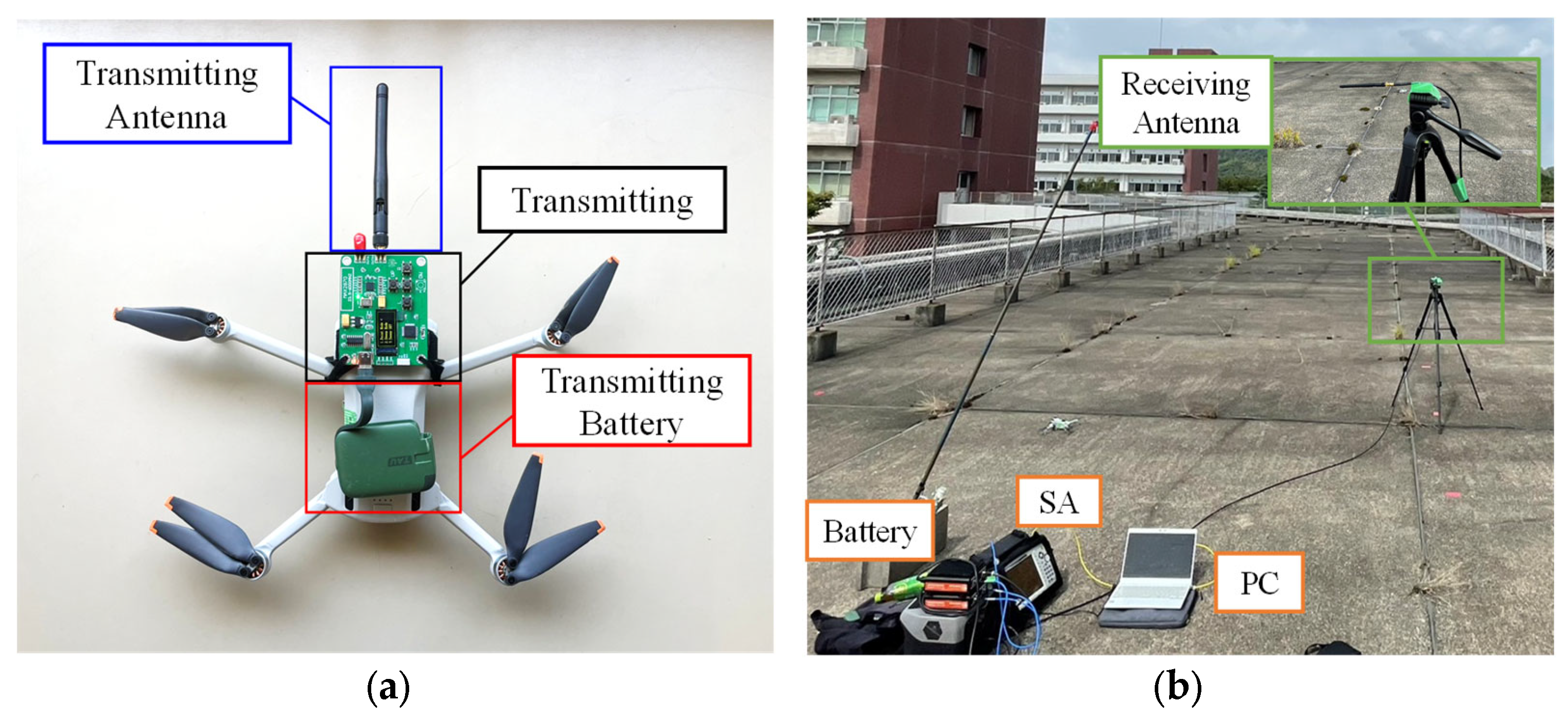
2.1. Radio Propagation Measurement Setup

As the 2.4 GHz band is widely used for UAV control, we measured the received power from the UAV to the ground at 2.5 GHz and evaluated the propagation characteristics. We introduce the configuration of the propagation measurement equipment in A2G communication using the UAV. Figure 1a shows the small UAV (DJI Mavic Mini 3) [42] used in this study. In this study, this UAV was used as a transmitter station and was equipped with a transmitter, a transmitter battery, and a half-wavelength dipole antenna as the transmitting antenna. To ensure the safety of the surrounding area, the UAV flew while tethered to a fishing line.

Figure 1b shows the receiver system on the ground. A half-wavelength dipole antenna was used as the receiving antenna, and a standard spectrum analyzer (SA) was used to measure the received power. The results measured by the SA were imported into a personal computer (PC), and the radio wave propagation characteristics, such as the cumulative distribution function (CDF) characteristics of measured instantaneous response and the Rician K-factor, were analyzed.

2.2. Radio Propagation Measurement Environment

In this study, to clarify the propagation characteristics of A2G communication in different environments, we selected two propagation environments on the campus of the University of Toyama. Figure 2 shows two environments using aerial imagery from Google Earth [43]. The simple propagation environment (S environment) is an area with a building but almost no obstructions in the surrounding area. In contrast, the complex propagation environment (C environment) is an area surrounded by buildings that have balconies and windows in the wall facing the propagation environment. These two environments were chosen to clearly evaluate the differences in propagation characteristics between S and C environments.

To accurately understand the propagation characteristics, measurement settings were made according to each environment as detailed in

Table 2. Radio propagation measurement parameters.

Parameter	Simple Propagation Environment		Complex Propagation Environment
Measurement time	5 s		10 s
Migration length L	1.5 m		3 m
Movement speed of UAV v	0.3 m/s
UAV altitude H	10–30 m
Distance between the nearest building and transmitting antenna (UAV) Dt	5 m	10 m	5 m
Distance between the nearest building and receiving antenna Dr	5 m	10 m	15 m
Frequency f	2.5 GHz
Transmitting antenna	Half-wavelength dipole antenna
Receiving antenna	Half-wavelength dipole antenna
Antenna arrangement	Horizontal installation		Horizontal installation	Vertical installation

. Radio wave propagation measurements are performed in a static environment without people or other moving objects, which ensures that the propagation paths are generally consistent. Changes in UAV attitude and position due to wind will cause changes in the scattered path power, so the received signal may fluctuate slightly, but drastic changes such as fading are not expected. In such cases, the Rician K-factor cannot be accurately estimated from the measurement data. To cause fading at these points, either the transmitting or receiving station would have to be moved, so to simulate this, the UAV was flown. In each environment, the distance between the transmitting antenna mounted on the UAV and the nearest building was defined as D_t, whereas the distance between the receiving antenna on the ground and the nearest building was defined as D_r.

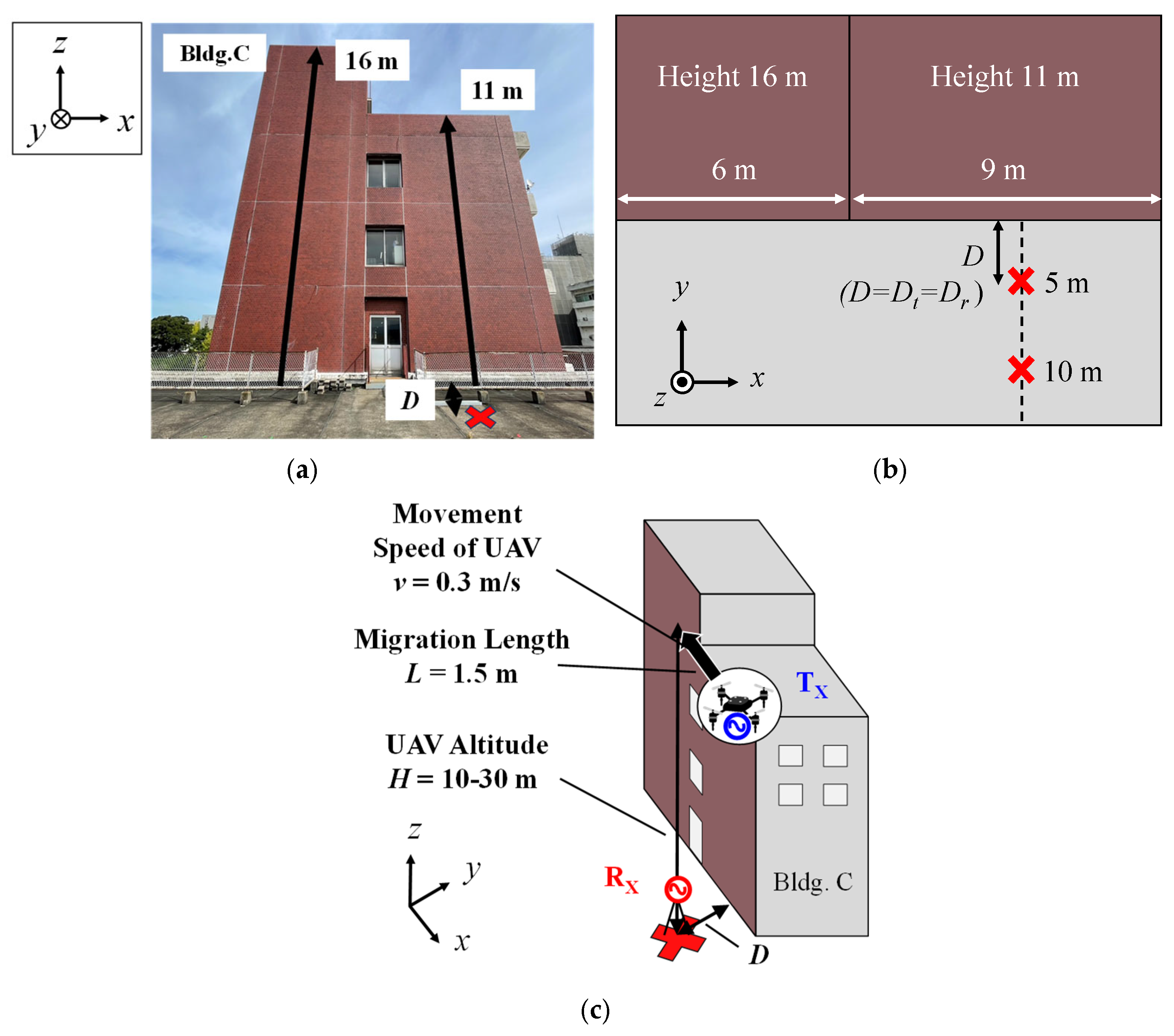
2.2.1. Simple Measurement Environment

Figure 3a shows a photograph of the selected S environment, where there is only one building. The building has different heights on the left (16 m) and right (11 m) sides. As shown in Figure 3a, the wall of Building C is made of brick, and there is one door and two windows in the center of Building C, but the overall structure of the walls is flat with few bumps and hollows. The location where the receiving antenna was placed is the rooftop of another building which is concrete.

Figure 3b depicts the top view of the measurement environment with a detailed diagram of each parameter. The distance D_t between the transmitting antenna and Building C and the distance D_r between the receiving antenna and Building C were set to the same distance, D. The transmitting and receiving points were located 5 m and 10 m from the center of the right-hand building as shown by the X marks in the figure. The receiving antenna was placed 1 m above the rooftop of another building. Half-wavelength dipole antennas were used for the transmitting and receiving antennas.

Figure 3c illustrates the flight path of the UAV which was moved along an axis parallel to the ground and Building C, i.e., the x-axis. The UAV flew at 5 m intervals from 10 m to 30 m above the ground. The migration length of the UAV was set to 1.5 m to reduce the variation in the spatial propagation loss component of the received signal during movement, and the movement speed of the UAV v was set to 0.3 m/s to eliminate as much as possible the effect of Doppler frequency.

2.2.2. Complex Measurement Environment

Figure 4a shows the photograph of the selected C environment, which is surrounded by buildings on all sides. The height of each building is as follows: Building A is 26 m, Building B is 18 m, Building C is 18 m, and Building D is 8 m. As shown in Figure 4a, these buildings have balconies and windows, and thus the diversity of the wall surface shapes is expected to cause complex reflections and scattering that will affect the propagation characteristics.

Figure 4b shows two antenna arrangements to achieve the different directivity characteristics in terms of the radiation pattern and the polarization. Horizontal installation is when the antenna elements are set parallel to the ground and Building A, resulting in a horizontal polarization of omnidirectional nature, whilst vertical installation is when the antenna elements are set perpendicular to the ground, resulting in a vertical polarization of figure-8 shape. In this way, it is possible to evaluate in detail the effects of the directivity and polarization characteristics of the antenna on the propagation characteristics.

Figure 4c depicts the top view of the measurement environment with a detailed diagram of each parameter. If the transmitting and receiving antennas have been set up for the vertical installation and D_t = D_r, the radiation gain of the transmitting and receiving antennas in the direction of the direct path decreases rapidly, as can be seen from the directivity of the transmitting and receiving antennas drawn in Figure 4b, so D_t and D_r were set to different distances. The UAV equipped with the transmitting antenna was flown parallel to Building A, and the center of its path was 15 m from Building B and 5 m from Building A. The receiving antenna was placed at a height of 1 m above the concrete pavement surface, 15 m from Building B, and at a distance of D_r = 15 m from Building A. Half-wavelength dipole antennas were used for the transmitting and receiving antennas.

Figure 4d illustrates the flight path of the UAV parallel to Building A at a flight distance of L = 3 m centered at D_t. This migration length was set to twice that of the defined S environment to consider the effect of the C environment on the propagation characteristics. The UAV altitude was changed in 5 m increments between 10 m and 30 m above the ground. The movement speed of the UAV v was set to 0.3 m/s.

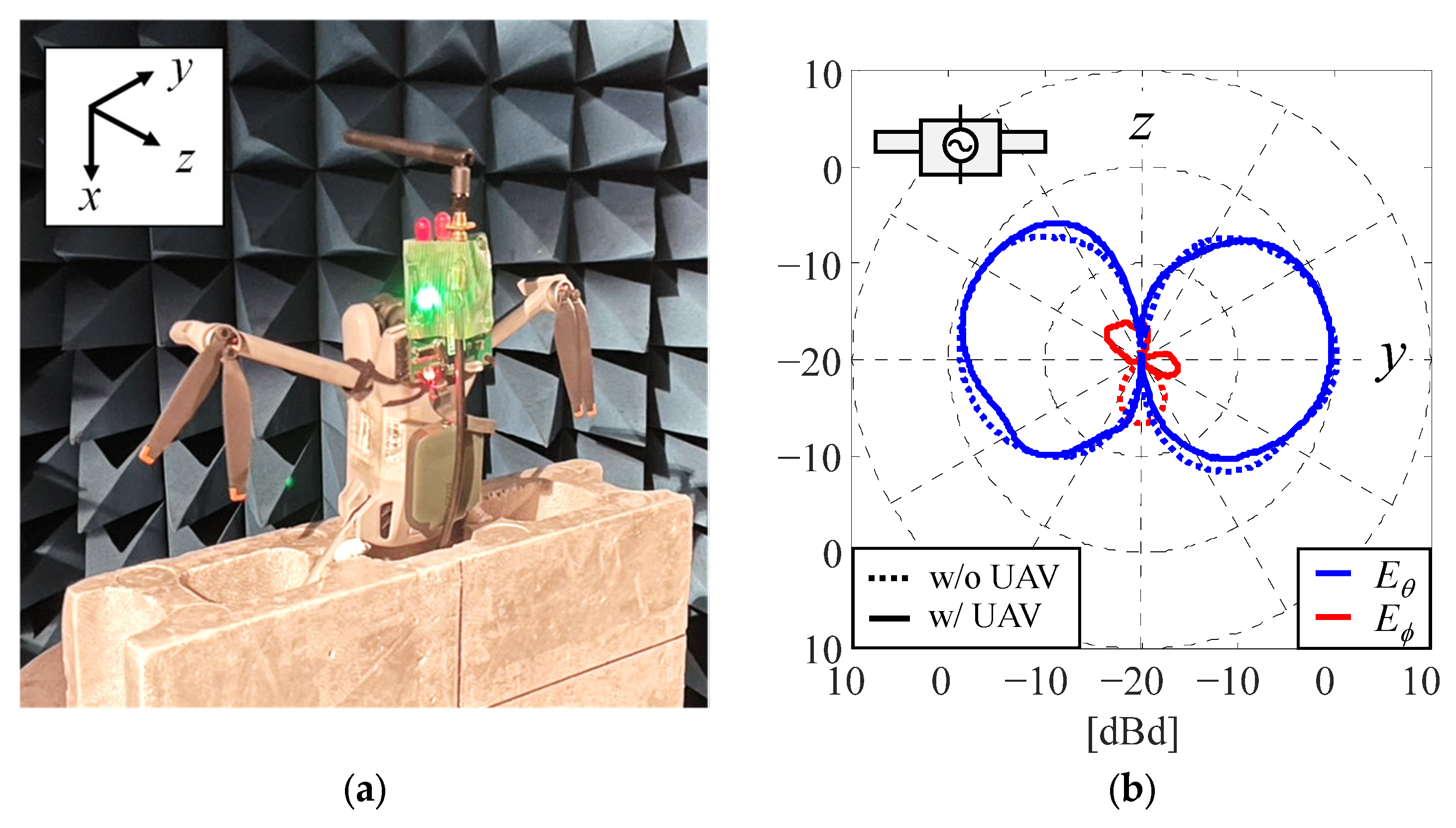
2.3. Directivity Evaluation Considering the UAV

To evaluate the effect of the UAV on the amplitude radiation pattern of the antenna when the transmitting antenna is mounted on the UAV, the directivity of the transmitting antenna was measured in an anechoic chamber. To assess the impact of building reflections on propagation, the directivity in the zy-plane of the used half-wave dipole antenna was measured. Figure 5 shows the amplitude radiation pattern of the antenna for a horizontal installation, while Figure 6 shows that for a vertical installation. Figure 6a and Figure 7a show the photograph of the measurement setup, while Figure 6b and Figure 7b show the measured radiation pattern in the zy-plane. The solid and dashed lines represent the radiation patterns with and without the UAV, respectively. The blue and red lines represent the E_θ and E_Φ components, respectively.

As can be seen from Figure 5, comparing the measured radiation pattern with and without the UAV, the E_θ and E_Φ components are generally the same. In addition, the E_Φ component is omnidirectional in the zy-plane, so communication is possible both in the air and the ground directions, i.e., the z-axis.

As shown in Figure 6, the radiation pattern with the UAV matches that without the UAV. However, communication in the air and the ground directions is not possible because the radiation pattern of the E_θ component is a figure-8 shape. From the measurement results shown in Figure 5 and Figure 6, the UAV used for the measurements did not affect the directivity of the transmitting antenna.

3. Radio Wave Propagation Analysis

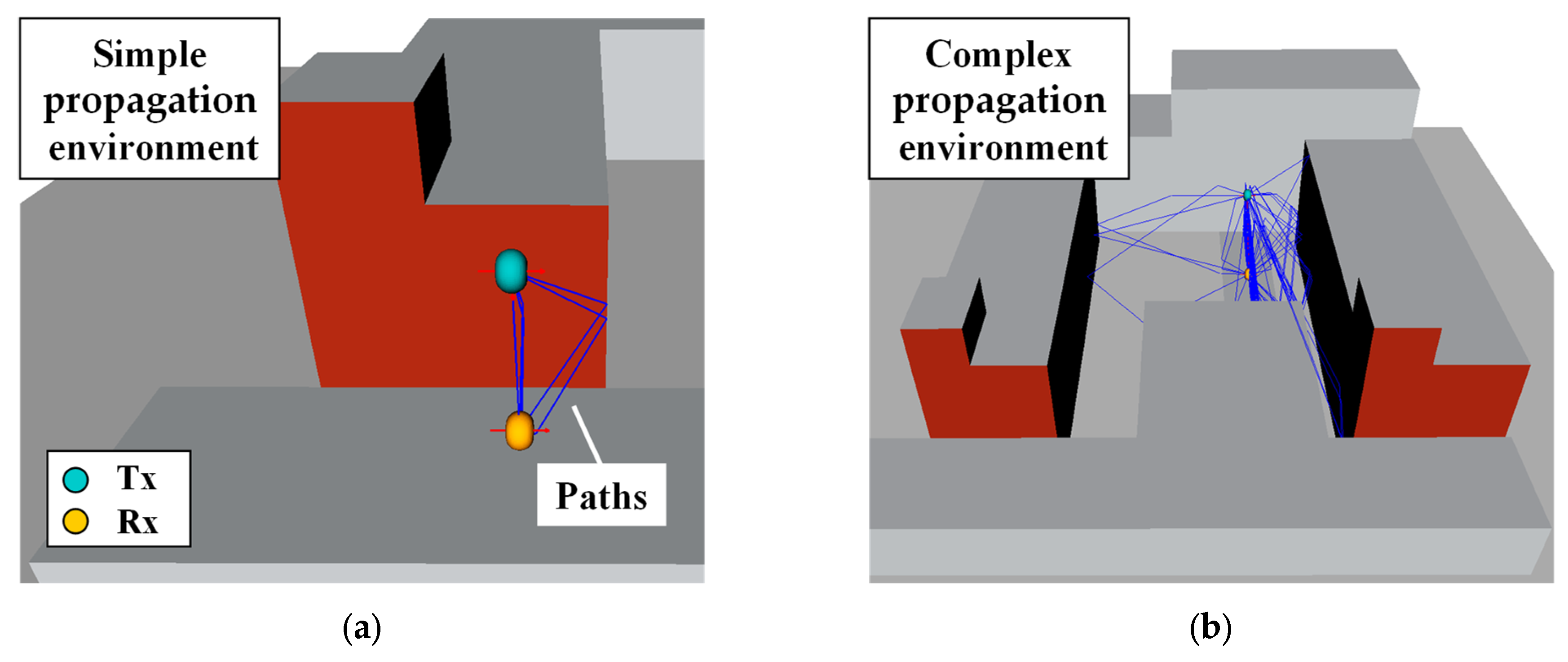
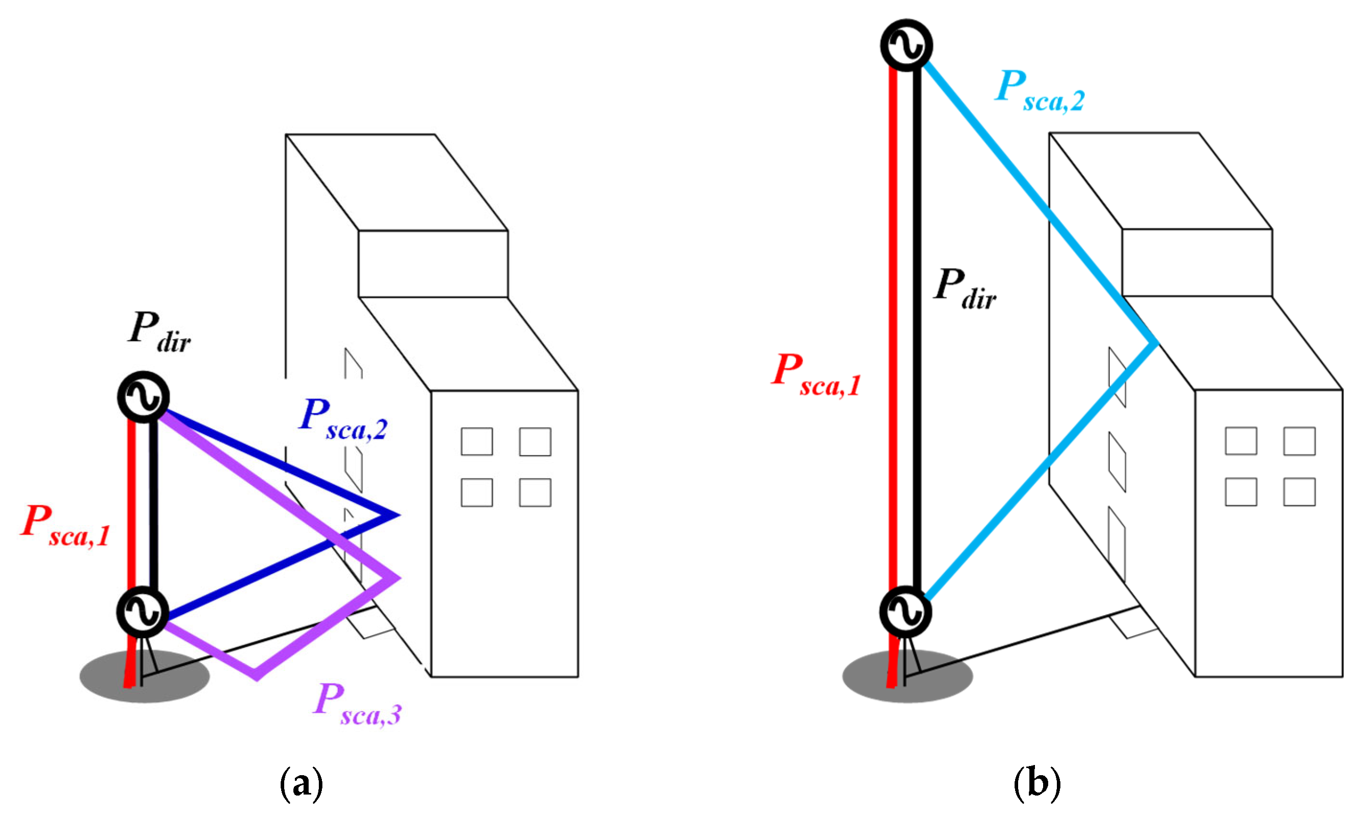
3.1. Channel Analysis Based on the Ray-Tracing Method

Figure 7 shows a simple 3D analytical model in which the rectangular parallelepipeds were combined to simulate S and C environments. Figure 7a,b are the analytical models of S and C environments, respectively. As shown in Figure 3a, the wall in the C environment has both a door and windows, but these are not considered in the analytical model. The wall painted red in the figure was made of bricks, and the other walls and the ground were made of concrete. As shown in Figure 4a, the buildings have many balconies and windows, but these are not considered in the analytical model, and the walls were modeled flat, so the path analysis does not account for building penetration losses. In addition, the trees between the measurement point and Building C are not considered. All the walls of the buildings and the ground were made of concrete.

The analytical parameters are shown in

Table 3. Configurations of the analysis.

Parameter	Simple Propagation Environment	Complex Propagation Environment
Frequency f	2.5 GHz
Transmitting antenna	Half-wavelength dipole antenna
Receiving antenna	Half-wavelength dipole antenna
Ground material	Concrete
Relative permittivity εr	5.31
Conductivity ρ [S/m]	0.194
Wall material	Brick	Concrete
Relative permittivity εr	3.91	5.31
Conductivity ρ [S/m]	0.024	0.194
Maximum number of reflections	3
Maximum number of diffractions	1

. The relative permittivity ε_r of the brick was set to 3.91, and the conductivity ρ was set to 0.024 S/m, based on the ITU-R recommendation [44]. The relative permittivity ε_r and conductivity ρ of the concrete were set to 5.31 and 0.194 S/m, respectively. The maximum number of reflections and diffraction were set to three and one, respectively. The frequency in the analysis was 2.5 GHz, and half-wave dipole antennas were used as the transmitting and receiving antennas.

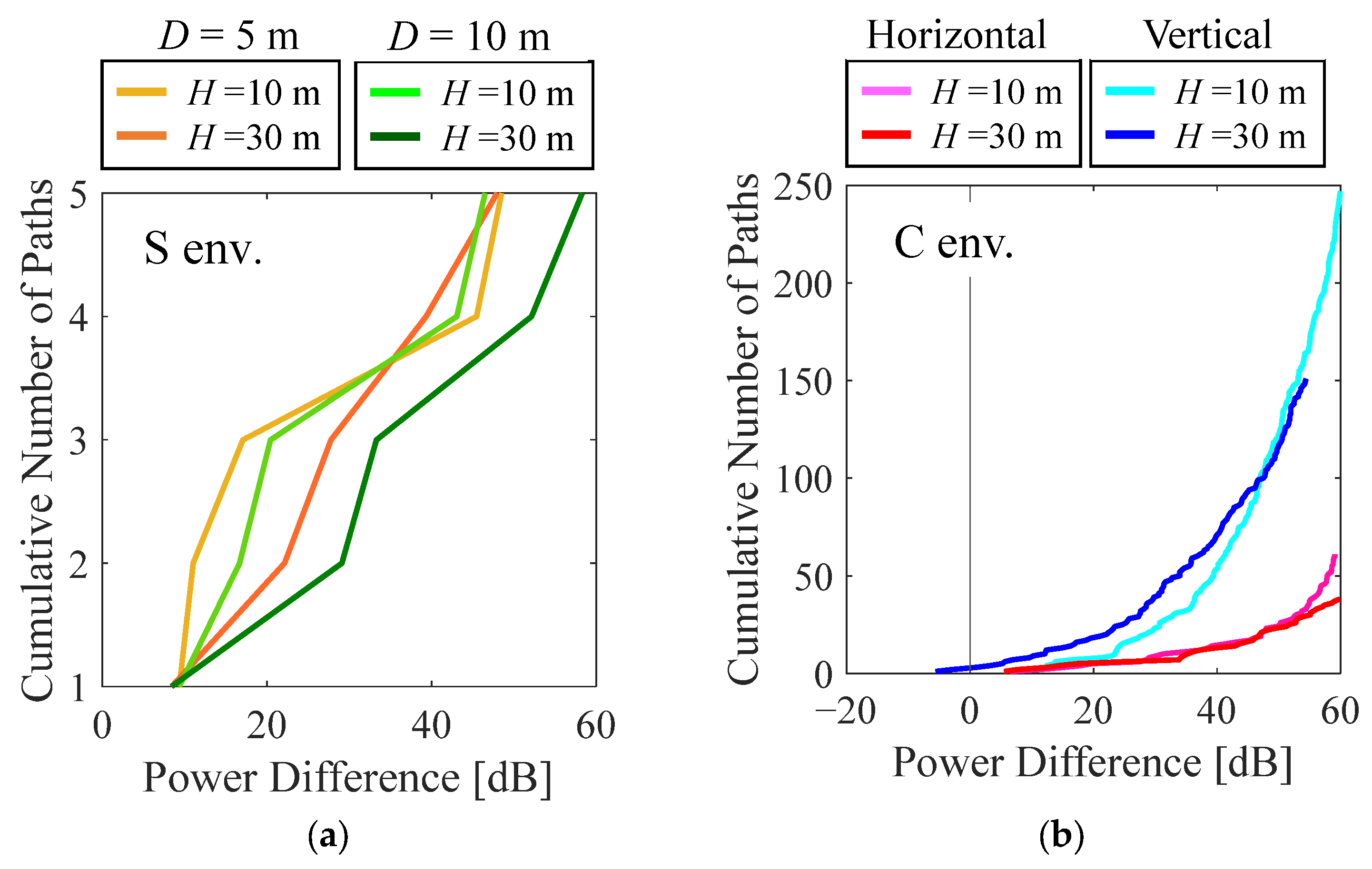
3.2. Results of the Channel Analysis

We performed radio wave propagation analysis using the ray-tracing method of RapLab (Kozo Keikaku Engineering Inc., Tokyo, Japan) [45] using the created model. The transmitting and receiving antennas in the analysis were placed in the same locations as in the measurements. Among the calculation results using the ray-tracing method, we focused mainly on the following items: the received level between both ends of the transmitting and receiving antennas, the direction and path power of the direct wave, and the direction and path power of each scattered wave. Here, the received level and path power include spatial loss and the radiation gain in the direction of the incoming wave in the transmitting and receiving antennas.

As an example of the analytical results, the path for D = 5 m and H = 10 m in the S environment is shown in Figure 7a, while the path for horizontal installation and H = 10 m in the C environment is shown in Figure 7b. The shapes drawn in green and yellow show the directivity of the transmitting and receiving antennas which are the half-wavelength dipole antennas. The blue lines show the paths with a power difference of less than 60 dB from the direct wave. It can be seen from Figure 7a that the number of paths shown is very small because there is only one building in the propagation environment. In contrast, as shown in Figure 7b, there are a lot of scattered waves through surrounding buildings. Hence, it is expected that the received power will vary greatly depending on the environment.

Figure 8 shows the cumulative number of paths up to the power difference defined as that between the direct wave and each scattered wave. This analysis focused on the cases with the shortest and longest distance between the UAV and the receiving antenna, at altitudes of H = 10 m and H = 30 m. Figure 8a,b show the results for the S and C environments, respectively.

To support the results of Figure 7, the cumulative number of paths up to the power difference in Figure 8b is quite a bit larger than that in Figure 8a regardless of the analysis conditions. A possible reason for this trend is that there are many scattered waves caused by surrounding buildings.

As shown in Figure 8a, the cumulative number of paths up to the power difference of H = 10 m (yellow and yellow-green lines) is greater than that of H = 30 m (orange and green lines) regardless of the distance between the antenna and Building C. The reason is that when H = 10 m, the scattered waves arriving at the receiving antenna, except for the single reflection from the ground which has the largest path power, are the reflected waves through Building C. In contrast, when H = 30 m, the scattered waves, except for the single reflection from the ground, are the diffracted waves through Building C because the UAV altitude is more than twice the height of Building C, so the reflected waves through Building C do not impact the receiving antenna. Therefore, it can be considered that the diffraction loss is greater than the reflection loss.

As shown in Figure 8b, it was confirmed that the number of paths with a power difference of less than 60 dB from the direct wave in the vertical installation (light blue and blue lines) was much higher than that in the horizontal installation (pink and red lines). This is due to the fact that in vertical installation, the radiation gain of the transmitting and receiving antennas is high, and the pattern in the direction of the surrounding buildings is omnidirectional, i.e., the horizontal plane, so the receiving antenna is more likely to receive scattered waves generated by buildings. On the other hand, in the horizontal installation, the radiation gain of the transmitting and receiving antennas is small in the direction of Buildings B and C, so the receiving antenna is not expected to receive the scattered waves from Buildings B and C.

Moreover, there are paths with power greater than the direct wave at H = 30 m in the vertical installation. A possible cause of this phenomenon is that the direction of the transmitting antenna relative to the receiving antenna increases in elevation angle with increasing the UAV altitude. In the vertical installation, the radiation gain of the direction of the direct path is very small in both transmitting and receiving antennas, resulting in lower path power, whereas, in horizontal installation, it is large because of the omnidirectional pattern, resulting in higher path power. Therefore, it is expected that the Rician K-factor will decrease in the vertical installation because the combined path power of the scattered waves will be greater than the path power of the direct wave.

3.3. Dummy Fading Signal Generation Based on the Static Paths

The ray-tracing method via RapLab analyzes the incoming signals at the receiving antenna for each path generated by the reflections and diffraction and then calculates the received signal by combining these paths. Since the phase fluctuations that occur over time in each path are not taken into consideration, the received signal has static characteristics, and a fading signal cannot be obtained. To address this, the dummy fading signal was generated by combining the signals taking into account the phase fluctuation generated using uniform random numbers for each path between the transmitting and receiving antennas [46,47]. Although the speed of the UAV is slow, the fading signal including the Doppler effect was still calculated using the following equation:

$$e\left(t\right)=\mathrm{Re}\left[{\displaystyle \sum _{i=1}^{N}r}i(t)\exp \left(j\left\{2\pi {\displaystyle \frac{vt}{\lambda }}\cos \alpha i+\theta i\right\}\right)\right]$$

(1)

where r_i denotes the amplitude of each path calculated using the ray-tracing method; v indicates the movement speed of the UAV; λ is the wavelength; α_i signifies the angle between the movement direction of the UAV and the arrival direction of the path; and θ_i is the random initial phase of [0, 2π).

There are many scattered paths with a power difference of 60 dB or more from the direct wave power, but it has been confirmed that the combined received power does not change significantly when the signal of these paths is added to the combined received power. Therefore, the combining received signal was calculated using N paths whose power difference from the direct wave was 60 dB or less. The dummy fading signal data were generated by performing this method at the same point and the same number of times as the sample points in the actual measurement.

As an example of the generated dummy fading signal, Figure 9 shows the received level at H = 10 m in the horizontal installation in the C environment. The red-purple line shows the result of the ray tracing according to the movement of the UAV, the black line shows the result of the dummy fading signal generated with Equation (1), and the blue line shows the measurement result.

As shown in Figure 9, the measurement result shows a large drop in received power, indicating that fading is occurring. The ray-tracing result shows no large drop in received power, and the received power fluctuates slightly around −60 dB, indicating that fading cannot be reproduced. In contrast, the dummy fading signal shows a large drop in received power, indicating that fading is being simulated.

The received power of the ray-tracing result and the dummy fading signal are roughly consistent with that of the measurement results but slightly higher. The reason for this difference in received power is that the radio propagation analysis was performed using a simplified 3D model shown in Figure 7, so it is assumed that the propagation environment was not sufficiently reproduced. However, it was found that the radio wave propagation analysis using a simplified 3D model was useful. A more detailed 3D model needs to be created and analyzed as a future research task.

3.4. Estimation of the Ricean K-Factor

All measurement environments of this study were LOS environments, so the Nakagami–Rice distribution is used to understand small-scale fading. The Rician K-factor, which evaluates fading behavior, can be used to evaluate communication stability. The Rician K-factor for the measurement results or analytical data generated with Equation (1) is estimated using the moment method expressed by the following equation [48]:

$$K={\displaystyle \frac{{\left|V\right|}^2}{{\left|v\left(t\right)\right|}^2}}={\displaystyle \frac{\sqrt{G{a}^2-G{v}^2}}{Ga-\sqrt{G{a}^2-G{v}^2}}}$$

(2)

where K indicates the estimated Rician K-factor; V denotes the direct wave signal; v(t) indicates the total scattered wave signal; G_a is the first moment of the power gain; and G_v is the second moment of the power gain about G_a, which is the root mean square (RMS) fluctuation. G_a and G_v are calculated from the measured and the analytical data generated with Equation (1).

Using the Rician K-factor estimated with Equation (2), the cumulative probability distribution curve was calculated from the following equation:

$$F\left(x;K\right)=1-Q_1\left(\sqrt{2K},\sqrt{2\left(1+K\right)x}\right)$$

(3)

where Q₁ is the Markov-Q function, which represents the Nakagami–Rice n distribution and can be expressed as follows:

$$Q_1\left(a,b\right)={\displaystyle {\int }_b^{\infty }x\exp \left(-\frac{x^2+a^2}{2}\right)I_0\left(ax\right)dx}$$

(4)

The zeroth-order Bessel function I₀ is expressed as follows:

$$I_0\left(z\right)={\displaystyle \sum _{k=0}^{\infty }\frac{1}{{\left(k!\right)}^2}}{\left({\displaystyle \frac{z}{2}}\right)}^{2k}$$

(5)

Figure 10 shows the CDF characteristics of the received power data in Figure 9 normalized by each median. The red-purple line shows the results of the ray-tracing analysis, the black line shows the outcome of the dummy fading signal generated with Equation (1), the blue line shows the measured data, and the gray line shows the cumulative probability distribution curve based on the Rayleigh distribution, which is an NLOS environment. The solid line is the CDF characteristic, and the dashed curve is the characteristic calculated with Equation (3) with the Rician K-factor estimated using the moment method.

As shown in Figure 10, the CDF characteristic of the measured data has a steeper slope than that of the Rayleigh distribution, so the estimated Rician K-factor is 4.94 dB, indicating that the effect of the direct wave can be confirmed. The ray-tracing result shows that the slope of the cumulative probability distribution is extremely steep and inconsistent with the measured results because the fading in the actual environment is not sufficiently reproduced, as seen in Figure 9. In addition, the estimated Rician K-factor is 14.54 dB, which is higher than that of the measured data. In contrast, the cumulative probability distribution of the dummy fading signal generated based on the path information calculated with the ray-tracing method is very similar to that of the measured data, indicating that the estimated Rician K-factor agrees with that of the experimental results.

The cumulative probability distribution of the measured and analytical data (solid line) generally agrees with the theoretical characteristic (dashed curve) based on the estimated Rician K-factor. But there is some discrepancy in the low signal power region. This discrepancy is due to the fact that when estimating the Rician K-factor using the first moment and RMS, if the number of sample points is small, the estimation error can be large for small values of the cumulative probability distribution value [48].

4. Rician K-Factor Characteristics

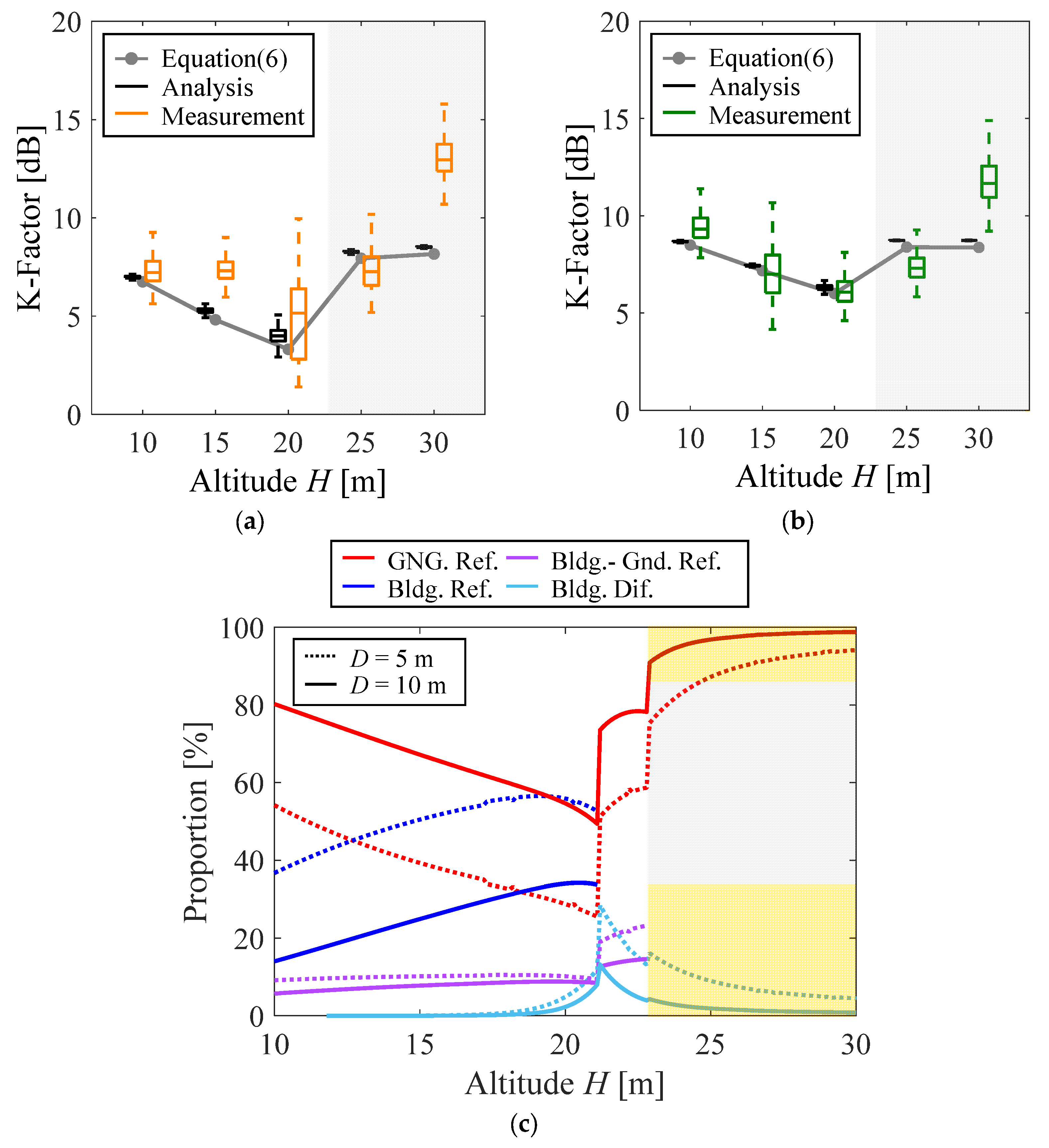
4.1. Rician K-Factor in Simple Propagation Environment

Figure 11 shows the difference in the main paths with high path power calculated using the ray-tracing method according to the UAV altitude in the S environment. Figure 11a,b show the results at H = 10 m and H = 30 m, respectively. The black line is the direct wave, the red line is the ground reflection wave, the blue line is the building reflection wave, the purple line is the building–ground reflection wave, and the light blue line is the building diffraction wave.

Comparing Figure 11a,b, the result for H = 10 m shows that the scattered waves include the reflected waves from the building and the ground, while the results for H = 30 m show that there are no reflected waves from the building, and the scattered waves have turned into the diffracted waves from the building.

Figure 12 shows the characteristics of the Rician K-factor in the S environment as a function of the UAV altitude. Figure 12a,b show the estimated Rician K-factors using the moment method with the measured data and the dummy fading data, depicted as box-and-whisker plots, for D = 5 m and 10 m, respectively. The orange or green colors are the measured data, the black color is the analytical outcomes, and the gray line is the static Rician K-factor using the ray-tracing method.

The static Rician K-factor is calculated by adding up the power of each path obtained by the ray-tracing method, and it can be expressed based on the following equation:

$$K={\displaystyle \frac{P_{dir}}{{\displaystyle \sum _{i=1}^N{P}_{sca,i}}}}={\displaystyle \frac{P_{dir}}{{\displaystyle \sum _{i=1}^N{\left|r_i\right|}^2}}}$$

(6)

where P_dir is the direct wave power, and P_sca,i is the power of each scattered wave at the point where the distance between the UAV and the receiving antenna is the shortest along the moving path.

Figure 12c shows the contribution rate of maximum path power among the paths of each scattering type as seen in Figure 11 based on the ray-tracing results as a function of the UAV altitude. The red line shows the contribution rate of the ground reflection wave. The blue line shows the contribution rate of the building reflection wave. The purple line shows the contribution rate of the building and ground reflection wave. The light blue line shows the contribution rate of the scattered wave with building diffraction. The solid and dashed lines are the results at D = 10 m and 5 m, respectively. In the figure, there are no reflected waves from the building at the UAV altitudes shown in yellow (H > 22.8 m).

First, looking at the static Rician K-factor using the ray-tracing method, those are generally smaller than the median of the Rician K-factor estimated from the analytical results. This is because the denominator in Equation (6) represents the maximum power that can be calculated with the scattered waves, and since this power is reduced by considering the phase of each path, the Rician K-factor necessarily increases as the denominator becomes smaller. Therefore, the static Rician K-factor obtained using the ray-tracing method tends to be an underestimate.

Comparing Figure 12a,b, the Rician K-factor increases with increasing the distance between the antenna and the building. The path length of the ground-reflected wave is the same regardless of the distance D, but the contribution rate of the ground-reflected wave at D = 10 m is higher than that at D = 5 m, as shown in Figure 12c. This means that the path power of other scattered waves is low at D = 10 m. Therefore, the Rician K-factor becomes higher as the distance D increases, so stable A2G communication can be expected.

The Rician K-factors of the measured and analytical results decrease between H = 10 m and 20 m regardless of the distance from the building. Then, the contribution rate of building reflection also increases with increasing the UAV altitude. On the other hand, the Rician K-factor increases above H = 21 m because building reflections shown as the blue line in Figure 12c do not reach the receiving point. Moreover, the Rician K-factor increases above H = 25 m because the reflection waves through the building shown as the blue and purple lines in Figure 12c do not reach the receiving point, and then the contribution rate of the diffraction wave also decreases. This indicates that, as the UAV altitude increases, the contribution rate of ground reflection becomes very high, and the Rician K-factor increases and approaches a constant value. On the other hand, the received power decreases with increasing distance between the transmitting and receiving antennas. Therefore, it is essential to consider the trade-off between UAV altitude and received power when designing the communication system.

However, the Rician K-factor of the measured results at an H = 30 m is significantly higher than that of the analytical value. Moreover, it can be confirmed that the variance of the Rician K-factor of the measured values is larger than that of the analytical values, as shown in the box-and-whisker plots in Figure 12a,b. It has been suggested that various factors such as the surface properties of buildings, the reflective properties of the ground, and the vibration of the UAV can affect the propagation of the direct and scattered waves in real environments. Further verification is required to determine whether this is due to local variations in the scattered wave or measurement error.

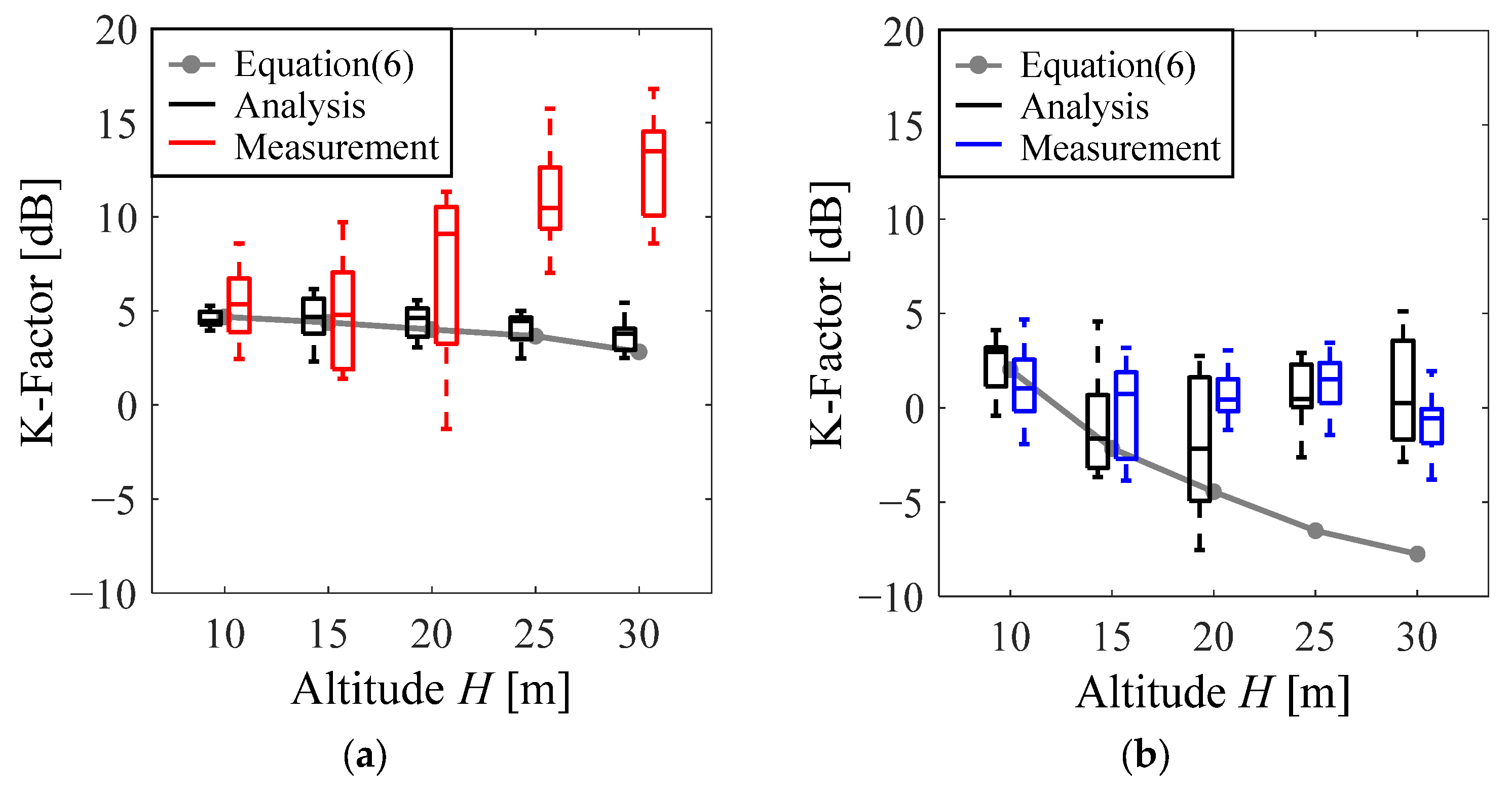
4.2. Rician K-Factor in Complex Propagation Environment

Figure 13 shows the Rician K-factor characteristics in the C environment as a function of the UAV altitude. Figure 13a,b show the results for horizontal and vertical installation, respectively. The estimated Rician K-factors using the moment method with the measured data and the dummy fading data are depicted as box-and-whisker plots with 12 data points for each altitude. The red or blue colors are the measured data, the black color is the analytical outcomes, and the gray line is the static Rician K-factor using the ray-tracing method.

As shown in Figure 13a, the Rician K-factors of the measured and analytical results decrease with UAV altitude from H = 10 m to 15 m. However, above H = 20 m, the Rician K-factor of the measured data increases, while the Rician K-factor of the analytical outcome decreases. A possible reason for this is that, as the UAV altitude increases, the incidence angle of the building reflection path increases. In measurement experiments, it is assumed that reflected waves through buildings can be attenuated or lost due to unevenness in the building walls, such as balconies and windows. As a result, the contribution rate of the scattered wave power is believed to have decreased, and the Rician K-factor has increased.

As shown in Figure 13b, the Rician K-factors of the measured and analytical results are the same regardless of the UAV altitude. The Rician K-factors of the measured and analytical results of the vertical installation are smaller than those of the horizontal installation, and more that of the variation of the analytical outcome is large. The reason for this will be explained in detail later using Figure 14.

Finaly, looking at the static Rician K-factor using the ray-tracing method, the results in the S environment are underestimated, just like those in the C environment. In particular, the static Rician K-factor using the ray-tracing method for vertical installations decreases significantly with increasing the UAV altitude, falling below 0 dB. In contrast, the values obtained from the simulation and measurements remain relatively constant at approximately 0 dB. This discrepancy is likely due to the limitations of the moment method used to estimate the Rician K-factor. Specifically, the moment method relies solely on the first moment, G_a, and the RMS, G_v, as defined in Equation (2). Consequently, it does not fully account for the power distribution between the direct wave and the scattered waves. A critical issue arises when the power of the direct path is less than the power of some scattered path, as shown in Figure 8b, so that the Rician K-factor becomes inaccurate.

Figure 14 shows a schematic diagram of the directivity of the transmitting and receiving antennas in horizontal and vertical installations at the zy-plane in the C environment. The red directivity is the E_Φ component in horizontal installation, while the blue directivity is the E_θ component in vertical installation. The black and gray lines indicate the direct wave at H = 30 m and H = 10 m, respectively. The light blue and green lines are the reflected wave from Building A at H = 30 m and H = 10 m, respectively.

It can be seen from Figure 14 that when the antenna is set to horizontal installation, the directivity is omnidirectional in the zy-plane, and the direct wave and the reflected wave from Building A are transmitted and received with the same radiation gain. However, the path power of the reflected wave from Building A is less than the power of the direct wave due to spatial losses along the path and losses due to reflection. Also, although not shown in the figure, the radiation gain of the transmitting and receiving antennas in the x-axis direction, where Buildings B and C are located, is very small, so the effect of the reflected waves from Buildings B and C is suppressed. Therefore, as shown in Figure 13a, it can be confirmed that the Rician K-factor is large, and the variation in the Rician K-factor by multiple measurements is small. In addition, it can be confirmed that the difference in path length between the direct wave and the reflected wave from Building A at H = 30 m is shorter than that at H = 10 m, indicating that the difference in path power between the direct wave and the reflected wave from Building A at H = 30 m is small. As a result, as shown in Figure 13a, it is considered that the Rician K-factor gradually decreases with the increase in the UAV altitude.

On the other hand, when the antenna is set to vertical installation, the directivity is a Figure 8 shape in the zy-plane. Since the transmitting and receiving directions change significantly depending on the UAV altitude, the radiation gain also changes. At H = 10 m, the direct wave and the reflected wave from Building A can be transmitted and received with relatively high radiation gain. In contrast, at H = 30 m, the radiation gain in the direction of both the direct wave and the reflected wave from Building A is small, so the received power of the direct wave and the reflected wave from Building A is low, even though the path is the same as in the horizontal installation. In addition, since the directivity in the xy-plane is omnidirectional and the radiation gain is high, the path power of the reflected waves not only from Building A but also from Buildings B and C increases, so the effect of the reflected waves from Buildings B and C is large. This makes the Rician K-factor extremely low.

It is concluded from these results that stable communication can be expected by setting to horizontal installation rather than vertical installation because the Rician K-factor is high.

5. Conclusions

In this paper, we conducted a detailed evaluation of the propagation characteristics of low-altitude A2G communication using UAVs. We clarified the effect of differences in the environment and the directivity characteristics of the antenna on the propagation characteristics. We conducted radio wave propagation measurements in a simple propagation environment (S environment) and a complex propagation environment (C environment). The following results were obtained, which will contribute to the establishment of optimal design guidelines for A2G communications.

The Rician K-factor was high in the S environment, reflecting the high stability of communication. In the C environment, the effects of multiple reflections and scattering were large, decreasing the Rician K-factor. This clearly showed the effect of the complexity of the environment on the propagation characteristics. In addition, we were able to specifically understand the impact of distance from the building and the UAV altitude on communication performance, highlighting the importance of this research.

By comparing horizontal and vertical installation of the antennas, we were able to accurately capture the changes in propagation characteristics due to the environmental conditions of radio wave propagation. Especially in the C environment, the communication performance was very stable with a horizontal installation, so it is important to pay attention to the antenna directivity. This finding will serve as a guideline for selecting the optimal polarization conditions for each environment in future communication system designs.

The results of this research can not only improve the performance of A2G communications using UAVs but also provide an important foundation for a variety of practical applications, such as ensuring communication during disasters and building effective networks in urban areas. However, this research was limited to evaluations in the 2.5 GHz, and an analysis of other frequency bands, more complex urban environments, and the dynamic characteristics of moving UAVs remain future challenges. It is expected that overcoming these challenges will further improve the versatility of UAV-based communication systems.

References

1. Zeng, Y.; Zhang, R.; Lim, T.J. Wireless Communications with Unmanned Aerial Vehicles: Opportunities and Challenges. IEEE Commun. Mag. 2016, 54, 36–42. [Google Scholar] [CrossRef]
2. Valavanis, K.P.; Vachtsevanos, G.J. (Eds.) Handbook of Unmanned Aerial Vehicles; Springer: Dordrecht, The Netherlands, 2015; ISBN 978-90-481-9706-4. [Google Scholar]
3. Mohsan, S.A.H.; Othman, N.Q.H.; Li, Y.; Alsharif, M.H.; Khan, M.A. Unmanned Aerial Vehicles (UAVs): Practical Aspects, Applications, Open Challenges, Security Issues, and Future Trends. Intel. Serv. Robot. 2023, 16, 109–137. [Google Scholar] [CrossRef] [PubMed]
4. Telli, K.; Kraa, O.; Himeur, Y.; Ouamane, A.; Boumehraz, M.; Atalla, S.; Mansoor, W. A Comprehensive Review of Recent Research Trends on Unmanned Aerial Vehicles (UAVs). Systems 2023, 11, 400. [Google Scholar] [CrossRef]
5. Höhrová, P.; Soviar, J.; Sroka, W. Market Analysis of Drones for Civil Use. LOGI Sci. J. Transp. Logist. 2023, 14, 55–65. [Google Scholar] [CrossRef]
6. Outay, F.; Mengash, H.A.; Adnan, M. Applications of Unmanned Aerial Vehicle (UAV) in Road Safety, Traffic and Highway Infrastructure Management: Recent Advances and Challenges. Transp. Res. Part A Policy Pract. 2020, 141, 116–129. [Google Scholar] [CrossRef]
7. Butilă, E.V.; Boboc, R.G. Urban Traffic Monitoring and Analysis Using Unmanned Aerial Vehicles (UAVs): A Systematic Literature Review. Remote Sens. 2022, 14, 620. [Google Scholar] [CrossRef]
8. Ham, Y.; Han, K.K.; Lin, J.J.; Golparvar-Fard, M. Visual Monitoring of Civil Infrastructure Systems via Camera-Equipped Unmanned Aerial Vehicles (UAVs): A Review of Related Works. Vis. Eng. 2016, 4, 1. [Google Scholar] [CrossRef]
9. Bruni, M.E.; Khodaparasti, S.; Perboli, G. Energy Efficient UAV-Based Last-Mile Delivery: A Tactical-Operational Model with Shared Depots and Non-Linear Energy Consumption. IEEE Access 2023, 11, 18560–18570. [Google Scholar] [CrossRef]
10. Sarvesh, E.; Jose, J.; Chitrakala, S. MedUAV: Drone-Based Emergency Medical Supply System Using Decentralized Autonomous Organization (DAO). Procedia Comput. Sci. 2023, 230, 737–748. [Google Scholar] [CrossRef]
11. 802.11-2012; IEEE Standard for Information Technology–Telecommunications and Information Exchange Between Systems Local and Metropolitan Area Networks—Specific Requirements Part 11: Wireless LAN Medium Access Control (MAC) and Physical Layer (PHY) Specifications; 802.11-2012 (Revision of IEEE Std 802.11-2007). IEEE: New York, NY, USA, 2012; pp. 1–2793. [CrossRef]
12. 802.11-2020; IEEE Standard for Information Technology–Telecommunications and Information Exchange Between Systems—Local and Metropolitan Area Networks—Specific Requirements—Part 11: Wireless LAN Medium Access Control (MAC) and Physical Layer (PHY) Specifications—Redline; 802.11-2020 (Revision of IEEE Std 802.11-2016). IEEE: New York, NY, USA, 2021; pp. 1–7524.
13. Abdalla, A.S.; Marojevic, V. Communications Standards for Unmanned Aircraft Systems: The 3GPP Perspective and Research Drivers. IEEE Commun. Stand. Mag. 2021, 5, 70–77. [Google Scholar] [CrossRef]
14. Characteristics of Unmanned Aircraft Systems and Spectrum Requirements to Support Their Safe Operation in Non-Segregated Airspace. Available online: https://store.accuristech.com/standards/itu-r-report-m-2171?product_id=2824436&srsltid=AfmBOopUhuKXUvApb7cuZ-5l_olP0K_5Xo1QmBwM_WWJOUIIMR-Tqe1k (accessed on 23 December 2024).
15. Khawaja, W.; Guvenc, I.; Matolak, D.W.; Fiebig, U.-C.; Schneckenburger, N. A Survey of Air-to-Ground Propagation Channel Modeling for Unmanned Aerial Vehicles. IEEE Commun. Surv. Tutor. 2019, 21, 2361–2391. [Google Scholar] [CrossRef]
16. Mao, K.; Zhu, Q.; Wang, C.-X.; Ye, X.; Gomez-Ponce, J.; Cai, X.; Miao, Y.; Cui, Z.; Wu, Q.; Fan, W. A Survey on Channel Sounding Technologies and Measurements for UAV-Assisted Communications. IEEE Trans. Instrum. Meas. 2024, 73, 1–24. [Google Scholar] [CrossRef]
17. Mozaffari, M.; Saad, W.; Bennis, M.; Nam, Y.-H.; Debbah, M. A Tutorial on UAVs for Wireless Networks: Applications, Challenges, and Open Problems. IEEE Commun. Surv. Tutor. 2019, 21, 2334–2360. [Google Scholar] [CrossRef]
18. 3GPP. Study on Channel Model for Frequencies from 0.5 to 100 GHz; Technical Report (TR) 38.901, Version 14.0.0; 3rd Generation Partnership Project (3GPP). 2017. Available online: https://www.3gpp.org/ftp/specs/archive/38_series/38.901/ (accessed on 10 January 2025).
19. 3GPP. Enhanced LTE Support for Aerial Vehicles; Technical Report (TR) 36.777, Version 15.0.0; 3rd Generation Partnership Project (3GPP). 2017. Available online: https://www.3gpp.org/ftp/specs/archive/36_series/36.777/ (accessed on 10 January 2025).
20. Al-Hourani, A.; Kandeepan, S.; Lardner, S. Optimal LAP Altitude for Maximum Coverage. IEEE Wirel. Commun. Lett. 2014, 3, 569–572. [Google Scholar] [CrossRef]
21. Lin, X.; Yajnanarayana, V.; Muruganathan, S.D.; Gao, S.; Asplund, H.; Maattanen, H.-L.; Bergstrom, M.; Euler, S.; Wang, Y.-P.E. The Sky Is Not the Limit: LTE for Unmanned Aerial Vehicles. IEEE Commun. Mag. 2018, 56, 204–210. [Google Scholar] [CrossRef]
22. Mozaffari, M.; Saad, W.; Bennis, M.; Debbah, M. Unmanned Aerial Vehicle with Underlaid Device-to-Device Communications: Performance and Tradeoffs. IEEE Trans. Wirel. Commun. 2016, 15, 3949–3963. [Google Scholar] [CrossRef]
23. Wu, Q.; Zeng, Y.; Zhang, R. Joint Trajectory and Communication Design for UAV-Enabled Multiple Access. In Proceedings of the GLOBECOM 2017—2017 IEEE Global Communications Conference, Singapore, 4–8 December 2017; pp. 1–6. [Google Scholar]
24. Leite, D.L.; Alsina, P.J.; de Medeiros Campos, M.M.; de Sousa, V.A.; de Medeiros, A.A.M. Unmanned Aerial Vehicle Propagation Channel over Vegetation and Lake Areas: First- and Second-Order Statistical Analysis. Sensors 2022, 22, 65. [Google Scholar] [CrossRef]
25. Alzenad, M.; Yanikomeroglu, H. Coverage and Rate Analysis for Unmanned Aerial Vehicle Base Stations with LoS/NLoS Propagation. In Proceedings of the 2018 IEEE Globecom Workshops (GC Wkshps), Abu Dhabi, United Arab Emirates, 9–13 December 2018; pp. 1–7. [Google Scholar]
26. Al-Hourani, A.; Kandeepan, S.; Jamalipour, A. Modeling Air-to-Ground Path Loss for Low Altitude Platforms in Urban Environments. In Proceedings of the 2014 IEEE Global Communications Conference, Austin, TX, USA, 8–12 December 2014; pp. 2898–2904. [Google Scholar]
27. Michailidis, E.T.; Nomikos, N.; Trakadas, P.; Kanatas, A.G. Three-Dimensional Modeling of mmWave Doubly Massive MIMO Aerial Fading Channels. IEEE Trans. Veh. Technol. 2020, 69, 1190–1202. [Google Scholar] [CrossRef]
28. Matolak, D.W.; Sun, R. Air–Ground Channel Characterization for Unmanned Aircraft Systems—Part III: The Suburban and Near-Urban Environments. IEEE Trans. Veh. Technol. 2017, 66, 6607–6618. [Google Scholar] [CrossRef]
29. Lyu, Y.; He, Y.; Liang, Z.; Wang, W.; Yu, J.; Shi, D. Measurement-Based Tapped Delay Line Channel Modeling for Fixed-Wing Unmanned Aerial Vehicle Air-to-Ground Communications at S-Band. Drones 2024, 8, 492. [Google Scholar] [CrossRef]
30. Cui, Z.; Briso-Rodríguez, C.; Guan, K.; Calvo-Ramírez, C.; Ai, B.; Zhong, Z. Measurement-Based Modeling and Analysis of UAV Air-Ground Channels at 1 and 4 GHz. IEEE Antennas Wirel. Propag. Lett. 2019, 18, 1804–1808. [Google Scholar] [CrossRef]
31. Bithas, P.S.; Nikolaidis, V.; Kanatas, A.G.; Karagiannidis, G.K. UAV-to-Ground Communications: Channel Modeling and UAV Selection. IEEE Trans. Commun. 2020, 68, 5135–5144. [Google Scholar] [CrossRef]
32. Fuschini, F.; Barbiroli, M.; Vitucci, E.M.; Semkin, V.; Oestges, C.; Strano, B.; Degli-Esposti, V. An UAV-Based Experimental Setup for Propagation Characterization in Urban Environment. IEEE Trans. Instrum. Meas. 2021, 70, 1–11. [Google Scholar] [CrossRef]
33. Qiu, Z.; Chu, X.; Calvo-Ramirez, C.; Briso, C.; Yin, X. Low Altitude UAV Air-to-Ground Channel Measurement and Modeling in Semiurban Environments. Wirel. Commun. Mob. Comput. 2017, 2017, 1587412. [Google Scholar] [CrossRef]
34. Khawaja, W.; Ozdemir, O.; Erden, F.; Guvenc, I.; Matolak, D.W. Ultra-Wideband Air-to-Ground Propagation Channel Characterization in an Open Area. IEEE Trans. Aerosp. Electron. Syst. 2020, 56, 4533–4555. [Google Scholar] [CrossRef]
35. Cai, X.; Rodríguez-Piñeiro, J.; Yin, X.; Wang, N.; Ai, B.; Pedersen, G.F.; Yuste, A.P. An Empirical Air-to-Ground Channel Model Based on Passive Measurements in LTE. IEEE Trans. Veh. Technol. 2019, 68, 1140–1154. [Google Scholar] [CrossRef]
36. Ning, B.; Li, T.; Mao, K.; Chen, X.; Wang, M.; Zhong, W.; Zhu, Q. A UAV-Aided Channel Sounder for Air-to-Ground Channel Measurements. Phys. Commun. 2021, 47, 101366. [Google Scholar] [CrossRef]
37. Mao, K.; Zhu, Q.; Qiu, Y.; Liu, X.; Song, M.; Fan, W.; Kokkeler, A.B.J.; Miao, Y. A UAV-Aided Real-Time Channel Sounder for Highly Dynamic Nonstationary A2G Scenarios. IEEE Trans. Instrum. Meas. 2023, 72, 1–15. [Google Scholar] [CrossRef]
38. Cui, Z.; Briso, C.; Guan, K.; Matolak, D.W.; Calvo-Ramírez, C.; Ai, B.; Zhong, Z. Low-Altitude UAV Air-Ground Propagation Channel Measurement and Analysis in a Suburban Environment at 3.9 GHz. IET Microw. Antennas Propag. 2019, 13, 1503–1508. [Google Scholar] [CrossRef]
39. Rodríguez-Piñeiro, J.; Domínguez-Bolaño, T.; Cai, X.; Huang, Z.; Yin, X. Air-to-Ground Channel Characterization for Low-Height UAVs in Realistic Network Deployments. IEEE Trans. Antennas Propag. 2021, 69, 992–1006. [Google Scholar] [CrossRef]
40. Cui, Z.; Guan, K.; Oestges, C.; Briso-Rodríguez, C.; Ai, B.; Zhong, Z. Cluster-Based Characterization and Modeling for UAV Air-to-Ground Time-Varying Channels. IEEE Trans. Veh. Technol. 2022, 71, 6872–6883. [Google Scholar] [CrossRef]
41. Aoki, K.; Honda, K. K-Factor Characteristics According to the Polarizations of Drone-to-Ground Communication. In Proceedings of the 2024 International Conference on Emerging Technology for Communications (ICETC), Kitakyushu, Japan, 25–27 November 2024. [Google Scholar] [CrossRef]
42. DJI Mini 3. So Fly. Available online: https://www.dji.com/global/mini-3?site=brandsite&from=landing_page (accessed on 23 December 2024).
43. Overview. Available online: https://www.google.com/earth/about/ (accessed on 23 December 2024).
44. P.2040: Effects of Building Materials and Structures on Radiowave Propagation above about 100 MHz. Available online: https://www.itu.int/rec/R-REC-P.2040-2-202109-S/en (accessed on 23 December 2024).
45. KKE―Innovating for a Wise Future. Available online: https://www.kke.co.jp/en/ (accessed on 23 December 2024).
46. Jakes, W.C. Microwave Mobile Communications; IEEE: New York, NY, USA; Wiley-Interscience: Hoboken, NJ, USA, 1994; ISBN 978-0-7803-1069-8. [Google Scholar]
47. Rappaport, T.S. Wireless Communications: Principles and Practice, 2nd ed.; Prentice Hall: Upper Saddle River, NJ, USA, 2001; ISBN 978-0-13-042232-3. [Google Scholar]
48. Greenstein, L.J.; Michelson, D.G.; Erceg, V. Moment-Method Estimation of the Ricean K-Factor. IEEE Commun. Lett. 1999, 3, 175–176. [Google Scholar] [CrossRef]
Figure 1. Radio propagation measurement setup: (a) UAV equipped with transmitter and antenna and (b) receiver system on the ground.
Drones 09 00086 g001
Figure 2. Radio propagation measurement environment from Google earth [43].
Drones 09 00086 g002
Figure 3. Simple measurement environment: (a) photograph of measurement environment; (b) top view of the analytical model and (c) flight path of the UAV.
Drones 09 00086 g003
Figure 4. Complex measurement environment: (a) photograph of measurement environment; (b) two antenna arrangements; (c) top view of the analytical model and (d) flight path of the UAV.
Drones 09 00086 g004
Figure 5. Directivity of the transmitting antenna in horizontal installation: (a) photograph of the UAV with the transmitting antenna and (b) amplitude radiation pattern in the zy-plane.
Drones 09 00086 g005
Figure 6. Directivity of the transmitting antenna in vertical installation: (a) photograph of the UAV with the transmitting antenna and (b) amplitude radiation pattern in the zy-plane.
Drones 09 00086 g006
Figure 7. 3D analytical model for the radio wave propagation simulation: (a) simple propagation environment and (b) complex propagation environment.
Drones 09 00086 g007
Figure 8. Cumulative number of paths for the power difference between the direct wave and each scattered wave: (a) simple propagation environment and (b) complex propagation environment.
Drones 09 00086 g008
Figure 9. Instantaneous received power for the horizontal installation at H = 10 m in a complex propagation environment.
Drones 09 00086 g009
Figure 10. Estimated Rician K-factor and cumulative distribution function for the horizontal installation at H = 10 m in a complex propagation environment.
Drones 09 00086 g010
Figure 11. Main paths in a simple propagation environment: (a) H = 10 m and (b) H = 30 m.
Drones 09 00086 g011
Figure 12. Radio propagation characteristics in a simple propagation environment: (a) estimated Rician K-factor at D = 5 m; (b) estimated Rician K-factor at D = 10 m and (c) proportion of each type of scattered wave.
Drones 09 00086 g012
Figure 13. Estimated Rician K-factor in a complex propagation environment: (a) horizontal installation and (b) vertical installation.
Drones 09 00086 g013
Figure 14. Radiation pattern of two antenna installations for each path angle in a complex propagation environment.
Drones 09 00086 g014