Abstract
In order to solve the problem of detecting, tracking and estimating the size of “low, slow and small” targets (such as UAVs) in the air, this paper designs a single-photon LiDAR imaging system based on Geiger-mode Avalanche Photodiode (Gm-APD). It improves the Mean-Shift algorithm and proposes an automatic tracking method that combines the weighted centroid method to realize target extraction, and the principal component analysis (PCA) method of the adaptive rotating rectangle is realized to fit the flight attitude of the target. This method uses the target intensity and distance information provided by Gm-APD LiDAR. It addresses the problem of automatic calibration and size estimation under multiple flight attitudes. The experimental results show that the improved algorithm can automatically track the targets in different flight attitudes in real time and accurately calculate their sizes. The improved algorithm is stable in the 1250-frame tracking experiment of DJI Elf 4 UAV with a flying speed of 5 m/s and a flying distance of 100 m. Among them, the fitting error of the target is always less than 2 pixels, while the size calculation error of the target is less than 2.5 cm. This shows the remarkable advantages of Gm-APD LiDAR in detecting “low, slow and small” targets. It is of practical significance to comprehensively improve the ability of UAV detection and C-UAS systems. However, the application of this technology in complex backgrounds, especially in occlusion or multi-target tracking, still faces certain challenges. In order to realize long-distance detection, further optimizing the field of view of the Gm-APD single-photon LiDAR is still a future research direction.
1. Introduction
In the field of aerospace monitoring and target tracking, precise detection, automatic tracking and accurate positioning of “low, slow and small” targets is a critical technical problem, especially in the environment of dynamic target movement; the complexity of this process is further increased [1,2]. The traditional target tracking algorithm (such as the Mean-Shift algorithm, the Particle-Filtering algorithm and the Sparse-Representation tracking algorithm) performs well in calculation speed and convergence [3,4,5,6]. However, many things could still be improved in its practical application. For example, this algorithm usually needs to select the target in the first frame manually. It cannot automatically adjust the tracking window and needs to show apparent improvements in the dynamic adjustment of target attitude and size [7,8]. At the same time, the existing detection technologies (including active radar early warning, electro-optical and infrared passive imaging cameras, acoustic and LiDAR) also have limitations in detecting “low, slow and small” targets. It is difficult to fully meet the needs of accurate positioning and size estimation [9,10,11,12].
Radar has strong penetration and long-distance detection ability. However, its spatial resolution is low, especially at low altitudes and close range, so it is difficult to provide enough details to locate small targets accurately [13,14,15]. Moreover, the detection performance of radar for slow or stationary targets could be better, and it is easily interfered with by background noise and clutter, thus affecting the accuracy of detection. With the outstanding performance of deep learning in various computer vision tasks and the widespread use of high-resolution cameras, it is now feasible to detect low-altitude UAVs based on passive imaging detection technology [16,17,18]. However, under insufficient, intense, or complex lighting, the detection effect will be reduced, and the accuracy and robustness of target detection are difficult to guarantee. Among them, the electro-optical camera can not directly provide the distance information of the target, which increases the difficulty of size estimation. Although the infrared camera can work effectively in low-light environments, its imaging resolution and details are often not as good as those of visible light cameras, and the detection effect is also lacking for low-speed small targets with weak infrared characteristics [19,20]. Acoustic detection uses acoustic sensors to search for acoustic waves (specific acoustic signals in the range of 0.3–20 kHz) generated by motors, propellers and other devices when the target flies and then compares them with the database’s audio to realize the target’s detection and classification [21,22,23]. The detection method based on acoustic waves has high robustness, but the detection distance is close (less than 200 m). It cannot be used in noisy environments, and its anti-interference ability is weak, so it is difficult to target micro and silent drones. Compared with radar and optical sensors, LiDAR has higher angular accuracy and distance accuracy, which can provide three-dimensional information about the target through laser beam scanning [24,25,26].
Abir, Tasnim Azad of the University of Texas, and others used a COTS lidar-based system (Livox Mid-40) to detect UAVs in airspace [27]. It successfully detected DJI Elf 4 UAV and DJI Inspire 2 UAV at 80 m and 50 m, respectively. This system’s longest detection distance for UAVs is 80 m. However, the ability of LiDAR to track UAVs in an extensive speed range is verified by the frame extraction method.
Sedat Dogru and Lino Marques used 3D LiDAR (16 vertical beams, 2 degrees apart, horizontal resolution ranging from 0.1 to 0.4 degrees, and corresponding frame rate ranging from 5 to 20 Hz) to obtain a sparse sample [25]. The system tracks the UAV with a size of 45 cm within 70 m in the airspace, and outputs the measurement value to compensate for the lost tracking through the tracking filter. The estimated tracking value of the system highly coincides with the real-time trajectory of UAV provided by the GNSS system, which verifies the possibility of LiDAR working all day to track UAV and LiDAR multi-system composite detection.
LiDAR has the ability to detect unmanned aerial vehicles all day and is not affected by environmental illumination. However, limited by short wavelength and the principle of multi-photon detection, the laser is affected by atmospheric absorption and scattering during its propagation, resulting in exponential attenuation of laser energy with propagation distance. On the one hand, water droplets in clouds, fog and rain will cause laser refraction and reflection, causing interference. On the other hand, due to less reflection of long-distance signals, the data are submerged in a lot of background noise, and the signal-to-noise ratio is extremely low, which also makes it difficult for LiDAR to effectively detect “low, slow and small” targets in a long distance.
Compared with the above methods, single-photon LiDAR has obvious technical advantages in detecting “low, slow and small” targets [28,29,30]. With the development of single-photon detector (SPD) and precision electronic timing technology, LiDAR based on time-correlated single-photon counting (TCSPC) was created [31]. Single-photon LiDAR is famous for its unique ability to detect and count a single-photon and has reached the theoretical detection limit. Unlike the traditional LiDAR, the single-photon LiDAR recovers the discrete waveform of the echo signal by time accumulation, thus obtaining the range and reflectivity information of the target. It has the advantages of high time resolution, high range resolution, anti-jamming ability, low energy consumption and long-distance detection, and can accurately measure the distance, shape and dynamic changes of the target, which is very suitable for real-time tracking and tracking of dynamic “low, slow and small” targets [32,33,34]. Compared with the electro-optical and infrared cameras, ambient illumination does not affect single-photon LiDAR. It can provide a stable monitoring effect during the day and night, in shadow areas, or during strong light interference [35].
Based on this background, this paper designs a single-photon LiDAR imaging system based on area array Geiger-mode avalanche photodiode (Gm-APD) [36,37], optimizes the Mean-Shift tracking algorithm [4], and proposes a tracking algorithm that combines the weighted centroid target extraction method and the principal component analysis (PCA) adaptive rotating rectangular frame fitting method to solve the problem of target attitude change and dynamic size adjustment [38]. This method not only realizes the automatic extraction and tracking of the target but also realizes the size estimation of the target through the high-precision ranging ability of the LiDAR, thus providing strong technical support for the accurate detection and automatic tracking of low-slow and small targets such as UAVs. Compared with the traditional sensor system, applying the improved algorithm to single-photon LiDAR shows the ability to detect and accurately track “low, slow and small” targets in real-time. We have also realized detection and tracking of the UAV at 1 km. Due to the large field of view of this radar, the optimized tracking algorithm in this paper realizes long-term and stable tracking.
The structure of this paper is as follows: Section 1 introduces the background of “low, slow and small” target detection and tracking in aerospace, Section 2 introduces a single-photon LiDAR imaging system based on area array Gm-APD designed by this paper, Section 3 introduces the improved tracking algorithm based on the Mean-Shift, Section 4 analyzes the improved algorithm’s dection and tracking results, and finally, the conclusion and prospects are presented.
2. Design of Single-Photon LiDAR Imaging System Based on Gm-APD
In order to realize the detection of “low, slow and small” targets (such as UAVs) in the air and space backgrounds, we designed and built an imaging system based on area array GM-APD LiDAR. The system consists of five subsystems: transmitting optical system, receiving optical system, GM-APD detector, data acquisition and processing system and servo system. Its design features are simple optical path, flexible operation and adjustment, which are suitable for detecting dynamic targets.
The core technical parameters of the system are as follows: the field of view of the LiDAR is 1.8°; the wavelength of the emitted laser is 1064 nm, output peak power is less than 10 W, and the repetition frequency is 20 kHz; The pixel number of the GM-APD detector is 64 × 64. Its workflow is divided into the following stages:
- Laser emission: Gm-APD LiDAR emits a high-power and narrow pulse laser, which is shaped by the optical launch system and accurately pointed at the target UAV;
- Echo signal reception: the echo photons reflected by the target are collected by the receiving optical system to the GM-APD detector, and the avalanche effect is triggered;
- Signal recording and transmission: GM-APD detector captures and records echo signals and transmits data to the data acquisition and processing system;
- Data processing and image reconstruction: The data acquisition and processing system processes the received signals and reconstructs the target’s intensity image and range image.
- Target tracking: An algorithm is applied based on image reconstruction results to realize target tracking.
In order to further highlight the insensitivity of active detection of single photon LiDAR in ambient illumination, the experimental time was cloudy and foggy in the morning, the illumination was 2219 lux, and the visibility was less than 3 km. Figure 1 shows the experimental test scene of Gm-APD single photon LiDAR detection, and the LiDAR is placed at a height of about 50 m (on the 16th floor). Figure 2 shows the detection and imaging results of DJI Elf 4 UAV in this airspace by the Gm-APD single photon LiDAR imaging system, in which the flying distance of Elf 4 UAV is less than 100 m, the flying height is less than 100 m and the flying speed is less than 5 m/s. The surface material of the fuselage is polycarbonate, and its fuselage size is 289.5 mm × 180 mm. The surface material of the wing is polypropylene, and the deployment size is 490 mm × 194 mm.
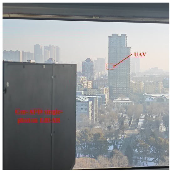
Figure 1.
The experimental test scene of Gm-APD single-photon LiDAR detection.
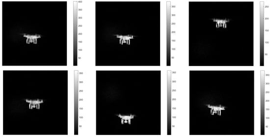
Figure 2.
Intensity imaging results of UAV detected by Gm-APD LiDAR.
Although the system has realized the actual imaging of UAV targets, as shown in Figure 2, due to the frequent dynamic changes in the UAV’s attitude during flight, the position and shape of the target fluctuate significantly in the intensity image, which makes tracking a problem. The fluctuation of imaging can be measured by the Euclidean distance between the real centroid position of the target and the centroid position fitted by the algorithm after imaging. The advantage of a target tracking algorithm based on Mean-Shift is that it needs few parameters, converges quickly in the iterative process, and does not require an exhaustive search [39]. However, the initial target area needs to be marked manually, and the search window is fixed, so it can not adapt to the spatial scale change of the target. The particle filter algorithm needs to build the state transition model of the target (such as speed, position change, etc.), which requires a large amount of computation and makes it difficult to meet the real-time requirements [40]. At the same time, if the motion characteristics of the target are inconsistent with the model assumptions (such as sudden acceleration or nonlinear motion), the tracking effect of the particle filter will be significantly reduced.
Therefore, we optimize the Mean-Shift tracking algorithm, use the weighted centroid method to extract the target, and combine the attitude estimation technology to improve the tracking accuracy, accurately estimate the actual size of the target, and finally realize automatic tracking.
3. Design of Automatic Tracking Algorithm Based on Mean-Shift
3.1. Principle of Mean-Shift Algorithm
The Mean-Shift algorithm is one of the most commonly used algorithms in target tracking. The local extremum is found in the density distribution of a data set through an iterative process. Because we do not need to know the probability density distribution function of the sample data, we only calculate the sample points. This function will converge when sampling is sufficient, so it has a relatively stable tracking effect [41]. Tracking steps include target model construction, candidate model construction, target similarity measurement, and Mean-Shift vector iteration [42].
3.1.1. Construction of Target Model
At the beginning of tracking, we must manually select the target in the Mean-Shift algorithm, build the target model, and select the appropriate parameters. Based on the LiDAR’s intensity image, we choose grey space to calculate the histogram of the target template, and n represents the number of pixels in the target template. At the same time, we choose the Epanechikov kernel function to calculate the kernel color histogram.
Therefore, the probability density estimation of the target template can be expressed as:
where k is the weighted sum profile function; h is the radius of the nuclear section; u is the color index corresponding to the histogram; is the normalized target position based on the target center; is the Kronecker function, which is used to determine whether the pixel value of is the u-th bin in the feature space; C is the standard normalized constant.
3.1.2. Construction of Candidate Target Model
In the subsequent frame of the target motion, the region that may contain the target is called the candidate region. Assuming that the target’s center position in the previous frame is , taking as the iterative starting point of the algorithm in the current frame, the center position y of the candidate target area is obtained, and the color feature distribution histogram of the current candidate area is calculated.
The candidate region centered on y has pixels, and each pixel is represented by , and the probability density of the candidate template is estimated as
3.1.3. Target Similarity Measurement
Similarity describes the degree of matching between the target and candidate areas after they are constructed. We use the Bhattacharyya coefficient [43,44] to measure the similarity between the candidate template and the target template, and its calculation formula is:
The Bhattacharyya distance is expressed as
The Bhattacharyya distance ranges from 0 to 1, and the larger the value, the more similar the two templates are. When the algorithm iteratively calculates to get the maximum value, the target’s actual position is the position at this time.
3.1.4. Mean-Shift Vector Iteration
We set the target center of the previous frame as the iteration starting point of the current frame as , iterate to find the best match from this point, and set the center position of the best matching area as y. The Formula (3) is expanded by the Taylor series at [45], and the Bhattacharyya coefficient can be approximately expressed as:
where represents the weight coefficient, which is determined by the size of the search window and the target position.
We can obtain the iterative formula of Mean-Shift as follows:
Among it, . The Mean-Shift algorithm starts from and calculates the Bhattacharyya coefficients of the target model and candidate model. The search box will grow to a new position of along the direction in which the density of the target pixel increases. After many iterations, until the moving distance is less than the set threshold, the actual position of the target in the current frame can be obtained, and tracking can be realized.
3.2. Algorithm Improvement
Because the Mean-Shift algorithm needs to manually extract and identify the target at the beginning of tracking, it is only suitable for semi-automatic systems. However, manual selection will seriously affect the algorithm’s real-time accuracy for a UAV target with a fast-moving speed and various state changes.
In addition, the principle of the Mean-Shift algorithm is mainly based on the grey feature distribution of images, that is, the intensity distribution information provided by the Gm-APD LiDAR, which also has the ability to obtain accurate three-dimensional spatial information of the target and provide the distance information of the target.
Therefore, we improve the Mean-Shift algorithm in this section, as shown in Figure 3, and propose a tracking method suitable for Gm-APD LiDAR. This method not only realizes the automatic calibration of the target but also accurately estimates the target size through its strength and distance information. At the same time, combined with the dynamic adjustment of the adaptive rotating rectangular frame, it can effectively solve the size estimation problem caused by target rotation and attitude change.
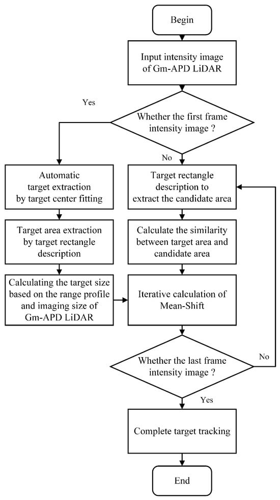
Figure 3.
Improvement of Mean-Shift tracking algorithm based on Gm-APD LiDAR.
The improved tracking method in this paper includes the following three main contents:
- Target center fitting algorithm;
- Drawing the target rectangle algorithm;
- Target size calculation algorithm.
These three algorithms will be described in detail below.
3.2.1. Target Center Fitting Algorithm
Based on the intensity imaging of the Gm-APD LiDAR, the laser echo signal contains complete information about the target, accompanied by some background stray light and noise. The existing methods of obtaining a target center can be roughly divided into two types: edge-based and gray-based.
As shown in Figure 4, we compare the fitting results of several methods for obtaining the target center. As shown in Figure 4a,b, edge-based methods (such as edge circle fitting [46] and Hough transform [47]) are suitable for large targets. These methods mainly rely on the contour information of the target and are insensitive to the grey distribution of the target. Therefore, when dealing with targets with small or large noise, its effect could be better, quickly leading to significant positioning error [48].
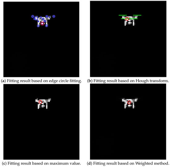
Figure 4.
Results of different center fitting methods based on Gm-APD LiDAR intensity imaging.
In contrast, the fitting methods based on the grey distribution (such as the maximum value method [49] and weighted centroid method [50,51]) are more suitable for dealing with small and relatively uniform grey distribution targets. This kind of method can capture the local grey features of the target, provide more accurate center positioning, and effectively improve the stability and accuracy of positioning, especially when dealing with an environment with intense noise. Among them, the maximum method is simple, but it relies too much on intensity information and ignores the target’s spatial structure and geometric distribution. Due to the sparsity of LiDAR data, substantial noise interference and uneven surface reflection, the maximum method (as shown in Figure 4c) often cannot provide accurate target center positioning. The weighted centroid method (as shown in Figure 4d) can make full use of the target’s grey level (intensity) information and combine the target’s spatial position to show better accuracy and robustness in small target locations and high noise environments.
Therefore, we use the weighted centroid method based on gray level (intensity) information and calculate the center of the target by giving weight to the intensity distribution of the imaging results, which effectively reduces the noise influence and improves the accuracy of extracting the center of the target. The calculation flow is shown in Figure 5.
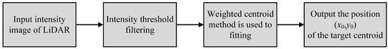
Figure 5.
Calculation flow of target centroid fitting.
The centroid calculation formula is as follows [52]:
where is the coordinate of a pixel of the intensity image of the LiDAR; is the intensity value corresponding to the pixel coordinate.
3.2.2. Drawing the Target Rectangle Algorithm
After the target center is obtained, we take this center as the rectangular center of the target rectangular frame and establish the circumscribed rectangular frame. Rectangular size directly affects the evaluation of target location, size, and threat level. The traditional rectangular frame with fixed size or simple minimum bounding rectangle makes it difficult to effectively deal with the target’s rotation, deformation, and size change at different angles and flight attitudes. Especially in the dynamic flight scene, the attitude change of the target will lead to the nonlinear transformation of its projection in the image, such as rotation and scaling.
In order to accurately describe the size and direction of the tracking rectangle, we propose an adaptive rotating rectangle fitting algorithm based on principal component analysis and weighted centroid calculation. By analyzing the edge point set of the target area, the algorithm accurately calculates its central direction. It dynamically adjusts the rotation angle of the rectangular frame, thus ensuring that the rectangular frame can be aligned with the actual shape and direction of the target. This can improve the accuracy of boundary fitting and maintain the stability and robustness of tracking when the target rotates or changes its attitude. The specific process is shown in Figure 6.
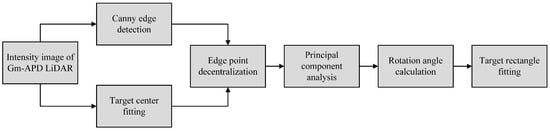
Figure 6.
Rectangular drawing algorithm flow.
- Firstly, the Canny edge detection algorithm [53,54] is used to extract the edge of the intensity image of Gm-APD LiDAR, and multi-level filtering and gradient calculation are carried out. Edge points can be accurately detected while reducing noise. The calculation flow is as shown in Figure 7.
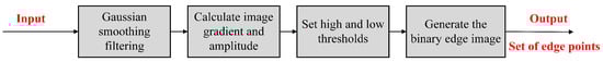 Figure 7. Calculation flow of edge fitting of intensity image.
- (a)
- Gaussian smoothing: The original intensity image is smoothed by a Gaussian filter to reduce the influence of noise on edge detection, and its mathematical expression is:where is a Gaussian filter and * is a convolution operation.
- (b)
- Gradient calculation: Calculate the gradient (amplitude and direction) of the image by the following formula to identify the target edge:where and represent the gradients of the midpoint in the X and Y directions, respectively.
- (c)
- Edge image: processing the gradient amplitude by setting high and low thresholds to generate a binary edge image of the LiDAR intensity image.
- To further analyze the spatial distribution characteristics of the target edge point set in the intensity image, the PCA method is introduced to accurately estimate the rotation angle of the rectangular box by calculating the principal direction of the edge point set [38,55]. The calculation flow is as shown in Figure 8.
 Figure 8. Calculation flow chart of PCA.
- (a)
- Constructing a centralization matrix D: decentralizing the edge points according to the weighted centroid fitted in the previous section further to determine the main direction of the edge points, and constructing a centralization matrix D:
- (b)
- Calculating covariance matrix ∑: the covariance matrix ∑ of matrix D is:
- (c)
- Eigenvalue decomposition: eigenvalue decomposition is performed on the covariance matrix ∑ to obtain the eigenvector corresponding to the maximum eigenvalue , the principal direction vector of the target edge point set. Therefore, the rotation angle in the main direction can be calculated by the following formula:
- After obtaining the central direction angle, the edge point set of the target is fitted by a rotating rectangle. The center of the fitted rectangle is still , and the width and height of the fitted rectangle are determined by the coordinate range of the edge points :
- Finally, use the rotation matrix R to rotate the corners of the fitted rectangle around the center of mass to the main direction:The corner coordinate of the fitted rectangle after rotation is:
This ensures the rectangle is aligned along the main direction of the target edge point set, that is, the moving direction of the target.
3.2.3. Target Size Calculation Algorithm
After calibrating the target center and drawing the adaptive rotating rectangular frame, we calculate the target’s actual size using the distance information provided by the range imaging of the Gm-APD LiDAR, the imaging size of the intensity image of the Gm-APD LiDAR and the LiDAR’s field of view angle (FOV) [56,57]. Because of the low spatial resolution of the radar, it is difficult to estimate the geometric size of the target accurately. At the same time, passive optical imaging technology (such as visible light camera and infrared camera, etc.) can only obtain two-dimensional image information and depend on external lighting conditions, which can not directly provide the depth information of the target. Therefore, the size estimation ability of these technologies in dynamic and complex scenes is limited. In contrast, single-photon LiDAR has high detection sensitivity at the photon level, which can emit a laser and receive feeble echo signals, accurately measure the distance between the target and the LiDAR, and obtain the three-dimensional spatial information of the target.
The FOV of the single photon LiDAR, the effective scanning angle, determines the spatial area that the Gm-APD detector can cover. The angular resolution represents the angular size of each pixel in the detector [58]. It determines the number of samples that can be returned in one scan and the minimum obstacle size that the LiDAR can detect. As shown in Figure 9, set the FOV as and the number of pixels as M × N. The corresponding angular resolution of each pixel can be expressed as:
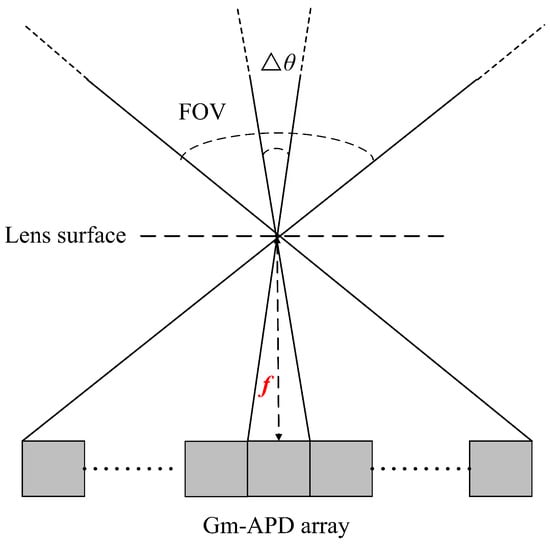
Figure 9.
Schematic diagram for calculating the FOV and angular resolution of LiDAR.
The Gm-APD detector we use satisfies M = N, so .
When the laser scans the target, the imaging size of the target is the projection of the actual size of the target in the LiDAR field of view. As shown in Figure 10, it is an imaging simulation diagram of a LiDAR detection target [59]. Set the focal length of the LiDAR receiving optical system as f and the detection distance from the target to the LiDAR as d.
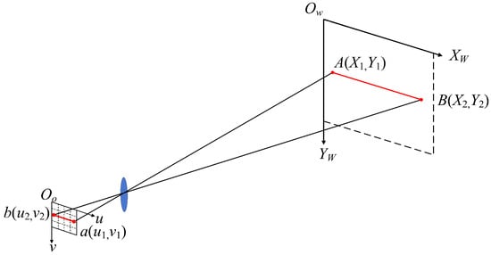
Figure 10.
Simulation diagram of LiDAR detection target.
For the world coordinate system and the detector coordinate system , the coordinates of any point and of the target in the world coordinate system are mapped to the coordinate and of the detector coordinate system through the projection relation, and the projection formula is:
When the target is located on a plane parallel to the optical axis of the LiDAR, that is , the projection relation section is further simplified as:
Correspondingly, the imaging size of the target on the detector is:
The total imaging size of the target on the detector can be expressed as:
From the proportional relationship between the imaging size of the detector and the imaging size of the world coordinate system, we can obtain the following:
Besides the formula for calculating the angular resolution of the detector mentioned above, it can also be expressed as the angle covered by each pixel on the detector. Defined as:
where is the physical size of each pixel on the detector.
Therefore, the imaging size of the target on the detector can be expressed as the product of the number of pixels and the size of a single pixel :
Substituting Equation (24) into the above formula, we can obtain:
The dimension calculation equation brought into the world coordinate system can be obtained:
When it is necessary to consider the nonlinear effect of high-order projection further and synchronize it with the drawing of the target rectangle algorithm, the distance d corresponding to the pixel point of the weighted centroid of the target is measured according to the LiDAR.
After changing the angular resolution from angle to radian information, the imaging size of the target in the Gm-APD LiDAR is through the target rectangular frame drawing, then the actual size of the target is further optimized as follows:
4. Analysis of Experimental Results
In this chapter, based on the Gm-APD single-photon LiDAR imaging system, we detect and image the DJI Elf-4 UAV in the airspace within 100 m (the flight speed is less than 5 m/s, and the flight attitude is dynamic hovering within the range of 50–100 m) and collect 1250 frames of image data to analyze the performance of the improved algorithm in this paper and the stability and accuracy of automatic tracking. The following items analyze the experimental results.
4.1. Analysis of the Results of Target Center Fitting Algorithm
In the target center positioning experiment, we intercepted 100 consecutive intensity images of the UAV’s level flying state (that is, the UAV’s motion posture is stable) and manually marked the center position of each frame of the target in this group of intensity images. The marking process is shown in Figure 11.
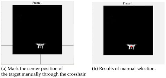
Figure 11.
Manual marking of target center position process.
At the same time, the improved centroid method proposed in Section 3.2.1 is compared with the traditional Hough transform method, the edge circle fitting method, the centroid method, and the maximum value method for target center fitting, and the fitting and manual marking results are shown in Figure 12.
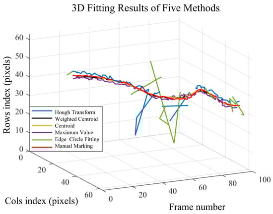
Figure 12.
Distribution of results based on various fitting methods of the target center position.
The imaging of Gm-APD LiDAR in 40 to 60 frames is shown in Figure 13. At this time, the corresponding UAV moves to the edge of the LiDAR’s field of view. In the imaging area of Gm-APD LiDAR, the effective signal (target signal) accounts for a small proportion, and the noise is more significant, thus affecting the accuracy of edge detection. The fitting method based on the Hough transform and edge circle is sensitive to noise, and the small imaging size is more easily disturbed by background noise, which leads to a significant fluctuation of fitting results. Therefore, these two methods have a significant deviation in this frame segment.
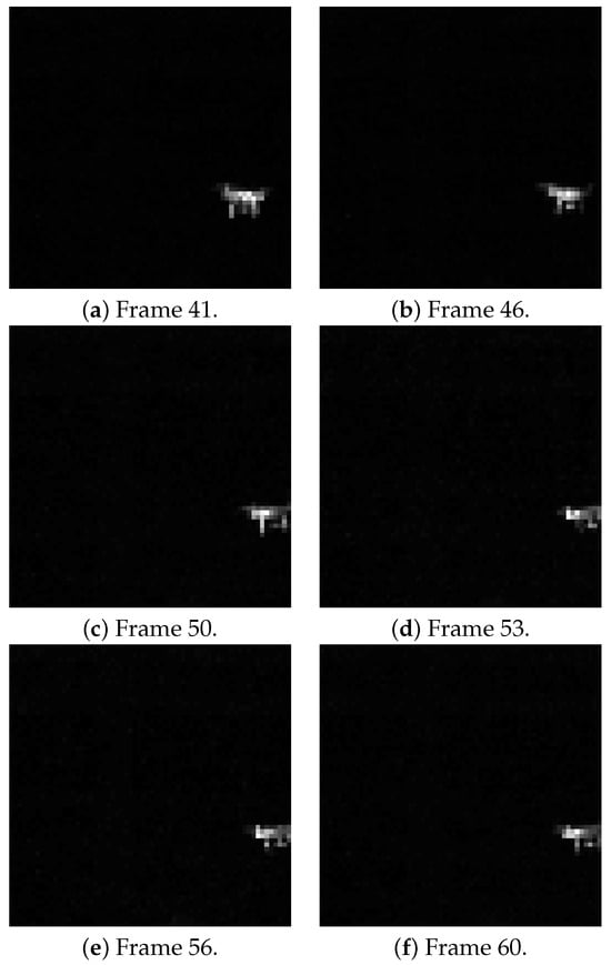
Figure 13.
Intensity imaging results of Gm-APD LiDAR in 40–60 frames.
At the same time, from the fitting effect, it can be intuitively seen that the maximum method, weighted centroid method, and centroid method have better fitting effects and can strike a balance between accuracy and stability, which conforms to the characteristics of the fitting method based on gray distribution mentioned in Section 3.2.1.
We further calculated the center location error (CLE) of the manual marking results corresponding to the centroid weighting method based on gray distribution, the maximum value method, and the centroid method, and the results are shown in Figure 14.
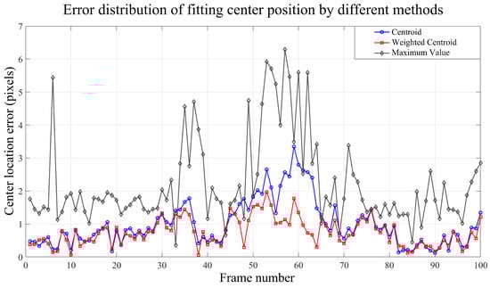
Figure 14.
Error distribution of multi-frame center positioning based on gray distribution fitting method.
Because the intensity image of LiDAR is influenced by the target material, surface characteristics, and distance of the UAV, the signal distribution is uneven and irregular. The maximum method only uses the highest intensity point, so it is more likely to be misled when the signal distribution is uneven, which makes its error fluctuate considerably. However, when the target boundary is blurred, the centroid method will be affected by the deviation of surrounding noise and deviate from the direction of noise concentration.
The previous description defines the imaging fluctuation as the Euclidean distance of the centroid position offset. During the dynamic flight of a UAV, the change in attitude may lead to the fluctuation of imaging results and cause the deviation of centroid fitting. In an ideal state, the centroid should accurately correspond to the center position of the UAV fuselage, and the center of the imaged rectangular frame is set as the projection position of the centroid. The centroid deviation will directly affect the measurement accuracy of the target size, so the centroid fitting error is strictly limited to one-fifth of the target size. At this flight distance of the UAV, this limit corresponds to an error range of about 3 pixels.
In most frames, the center positioning error value of the weighted centroid method is kept below 2 pixels. Compared with other methods, the weighted centroid method uses the intensity weight, which counteracts the influence of noise and background and shows high stability and accuracy.
4.2. Analysis of the Results of Drawing the Rectangular Frame of the First Frame Target
From the intensity imaging results of multi-frame LiDAR, we select the intensity imaging corresponding to the UAV’s oblique flight state (that is, the imaging results corresponding to the transformation of the UAV’s motion posture). Figure 15 and Figure 16 show the process and results of the rectangular box drawing algorithm based on Section 3.2.2.
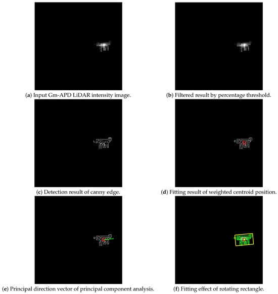
Figure 15.
The fitting results of the algorithm when the UAV changes its flight direction (flying to the left).
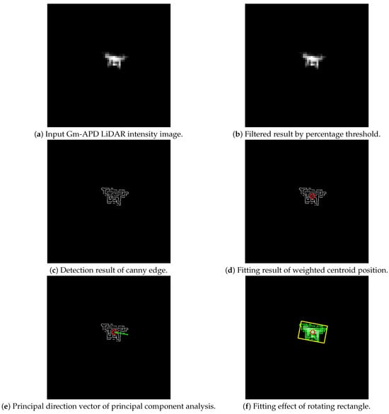
Figure 16.
The fitting results of the algorithm when the UAV changes its flight direction (flying to the right).
Figure 15d and Figure 16d show the target center fitting results when the UAV flies to the left and right, respectively. Even when the UAV’s attitude changes frequently, the target center acquisition algorithm can still maintain high stability and accurately capture the target’s center position, which shows that the algorithm has strong robustness in a dynamic environment.
Secondly, in the drawing of the rectangular frame, based on the center position of the target, the size (as shown in Figure 15e and Figure 16e) and direction (as shown in Figure 15f and Figure 16f) of the rectangular frame are dynamically adjusted by combining the PCA method to ensure that the rectangular frame can match the posture and shape of the UAV. The experimental results show that when the UAV changes its flight direction, the size and direction of the rectangular frame can well reflect the genuine attitude of the UAV, and it can adjust the angle adaptively and always keep alignment with the main direction of the target.
4.3. Analysis of Target Automatic Tracking Results
We apply the improved Mean-Shift tracking algorithm to realize the real-time automatic tracking of the UAV for 1250 consecutive frames. The tracking results are shown in Figure 17. The improved Mean-Shift algorithm can better characterize the target size and locate the tracking center accurately.
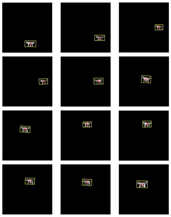
Figure 17.
Multi-frame tracking results based on improved Mean-Shift algorithm.
To evaluate the algorithm’s performance, we randomly selected 200 consecutive frames from the total number of frames collected and manually marked the center position of the UAV in these frames as the benchmark of the tracking algorithm. On this basis, we used the Kalman filter tracking algorithm [60,61], the algorithm combining Camshift and Kalman filter [62,63], and the improved algorithm proposed in this paper to track the target. The tracking center curve of each algorithm is shown in Figure 18.
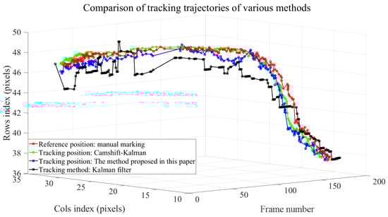
Figure 18.
Comparison of tracking trajectories of various methods.
The tracking results show that the Kalman filter (black) shows good stability in the stationary scene, but its effect is insufficient in the scene where the UAV is in nonlinear motion. Combining the adaptability of Camshift with the smoothness of the Kalman filter, this method can achieve relatively stable tracking in dynamic scenes, but its computational complexity is high. In contrast, the algorithm proposed in this paper only performs iterative calculations through MeanShift, which has the least computational burden. When the speed of the UAV is close to 5 m/s, due to the lack of Kalman filtering or other prediction methods to predict the target position, there will be some delay in the tracking process, resulting in a slight deviation compared with the Camshift and Kalman filtering method. However, the overall error is still within the acceptable range, which proves that this method has a good balance between accuracy and calculation efficiency.
Based on Section 3.2.1 and Section 3.2.2, Figure 19 shows the algorithm flow for obtaining the center of the first frame target of the LiDAR and drawing the rectangular frame, and Table 1 shows the specific distribution of the rectangular frame information.
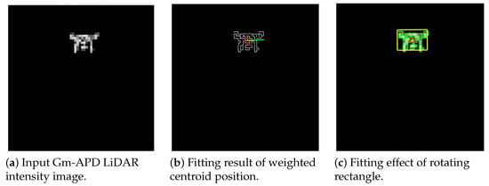
Figure 19.
First frame detection results based on improved Mean-Shift tracking algorithm.

Table 1.
Parameter distribution of tracking rectangular box.
At the same time, Figure 20 shows the range image corresponding to the first frame measured by the Gm-APD LiDAR system. According to the imaging results, the target distance is 51 m.
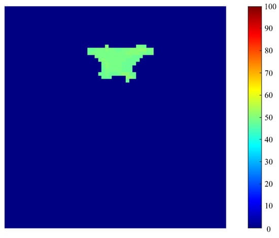
Figure 20.
The first frame range profile of Gm-APD LiDAR.
The field of view of the Gm-APD LiDAR designed in this paper is 1.8° × 1.8°, and the number of pixels of the Gm-APD detector is 64 × 64. Calculated by Equation (18), the corresponding field of view angle of each pixel is about 0.028°. The system allows the confidence interval of UAV tracking and rectangle drawing to be less than two pixels. Substituting the above parameters into Equation (28), the size of the target is calculated as 298.9 mm × 195.5 mm (W = 298.9 mm and H = 195.5 mm).
As shown in Figure 21, the physical object of DJI’s Elf 4 UAV is 289.5 mm × 180 mm, and its deployed size is 490 mm × 194 mm.
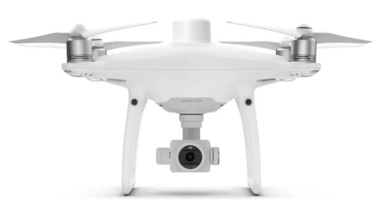
Figure 21.
Physical picture of DJI’s Elf 4 UAV.
The calculation result of the target size is between the UAV itself and the deployed size. The calculated dimensional error is within the confidence interval we set (less than 2.5 cm when converted to the dimensional dimension). As can be seen from the physical map, the paddle of DJI Elf-4 UAV has certain bending and flat characteristics. During the deployment process, the paddle may interfere with the laser light’s reflection characteristics, resulting in the LiDAR not accurately capturing every detail of the paddle. This phenomenon makes the propeller wing part show local expansion in laser imaging, which leads to the size obtained by LiDAR being between the size of the UAV itself and the expanded size of the propeller wing.
Therefore, this difference reflects the possible limitations of LiDAR in imaging complex geometric objects, especially when the detection target has a curved and thin structure.
The FOV of the single photon LiDAR built in this paper is fixed at 1.8 degrees, and the receiving optical system cannot zoom automatically with the flight distance of the target. With the increased flight distance of UAV, its imaging size in single photon LiDAR decreases significantly. Further, we have added a long-distance UAV flight experiment, where the flight distance of the UAV is between 700 and 1500 m and the flight speed is 10 m/s. The experimental time is 4 pm, the weather is cloudy, the visibility is 4 km, and the illumination is 3600 lux.
When the flight distance is 789 m, the imaging result of a single photon LiDAR is shown in Figure 22.
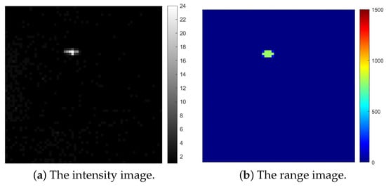
Figure 22.
Long-distance imaging results of single photon LiDAR (789 m).
When the flight distance is 949 m, the imaging result is as shown in Figure 23.
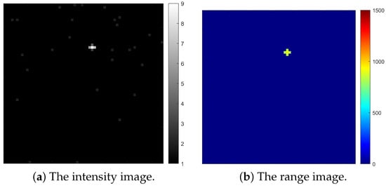
Figure 23.
Long-distance imaging results of single photon LiDAR (949 m).
When the flight distance exceeds 1.2 km, the imaging results are also shown in Figure 24.
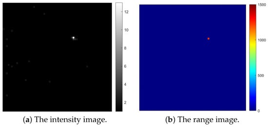
Figure 24.
Long-distance imaging results of single photon LiDAR (>1 km).
When the flight distance of the UAV exceeds 700 m, the tracking algorithm proposed in this paper can detect the imaging rectangular frame of the target and realize effective tracking. However, the intensity imaging information of the single photon LiDAR only appears as an effective pixel. With the further increase in flight distance, this phenomenon is more apparent, and the imaging result is always only a single pixel. Although the system can effectively detect the flight distance of a UAV, it can not obtain the specific imaging information of the UAV. The multi-frame results of tracking with the tracking algorithm proposed in this paper are shown in Figure 25.
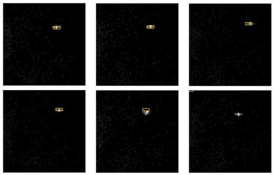
Figure 25.
Multi-frame tracking results based on improved Mean-Shift algorithm.
The tracking results show that the algorithm proposed in this paper can still track effectively in the first four frames, with a decrease in imaging pixels. At the beginning of the fifth frame, the tracking frame is off target, and the target tracking is lost. The single photon LiDAR system built in this paper can still effectively detect the UAV on long-distance flight. However, because there are too few imaging pixels and the target features are not obvious, the improved automatic tracking and size estimation algorithm based on Mean-Shift proposed in this paper can not track the UAV target. Moreover, due to the limitation of imaging information, the algorithm can not achieve accurate size estimation.
Therefore, the algorithm proposed in this paper is more suitable for UAVs flying at close range (less than 100 m) to ensure the effectiveness of the imaging and size calculation. In order to realize effective detection and imaging at a longer distance, the field of view angle of single photon LiDAR should be further reduced to ensure the number of pixels for UAV imaging.
5. Conclusions and Future Work
In this paper, a Gm-APD single-photon LiDAR imaging system is designed, and an improved automatic tracking and size estimation algorithm based on Mean-Shift is proposed. By optimizing the Mean-Shift algorithm, combining the weighted centroid method and the PCA method, the detection, tracking and size estimation of targets in dynamic scenes are realized. The experimental results show that the improved algorithm shows high fitting accuracy and tracking robustness in different flight attitudes of UAV, and can realize automatic acquisition, tracking and accurate size measurement of targets in the air and space background.
Compared with the traditional low-altitude detection methods, Gm-APD LiDAR has shown remarkable advantages in imaging and tracking low-slow small targets with its high detection sensitivity and high resolution. At present, the target region extraction of the algorithm is mainly based on the centroid method, which shows good performance when dealing with aerospace backgrounds or a single target. However, its applicability and robustness are significantly reduced in complex background conditions (such as urban and forest environments) and dealing with multi-target situations such as drone bee colonies. Therefore, introducing deep learning technology into target region extraction has become an important direction for future development. We plan to use deep learning methods, such as the Convolutional Neural Network (CNN) and Generative Countermeasure Network (GAN), to improve the detection accuracy of the algorithm for UAV targets. By labeling the imaging results of various UAVs and targets with “low and slow” characteristics (such as kites, birds, balloons, etc.), the accuracy of target recognition and classification of the system is further improved, thus significantly enhancing the robustness and practicability of the system.
The system has verified the feasibility of single-photon LiDAR in long-distance UAV detection. In the future, we will focus on optimizing the receiving optical system of single-photon LiDAR and ensuring that the UAV has enough pixels when imaging by reducing the system’s field of view to obtain more target information. These improvements will provide more reliable and accurate technical support for long-range UAV detection in complex scenes.
Author Contributions
Conceptualization, D.G. and Y.Q.; methodology, Y.Q. and X.Z.; software, J.L. and F.L.; validation, Y.Q., D.G. and S.Y.; formal analysis, D.G.; investigation, J.L. and F.L.; resources, D.G.; data curation, J.S. and X.Z.; writing—original draft preparation, D.G.; writing—review and editing, Y.Q. and J.S.; visualization, J.S.; supervision, Y.Q. and X.Z.; project administration, D.G. and J.S.; funding acquisition, J.S. All authors have read and agreed to the published version of the manuscript.
Funding
This research received no external funding.
Data Availability Statement
The original contributions presented in the study are included in the article, further inquiries can be directed to the corresponding author.
Conflicts of Interest
Authors Jie Lu and Feng Liu were employed by the company the 44th Research Institute of China Electronics Technology Group Corporation. The remaining authors declare that the research was conducted in the absence of any commercial or financial relationships that could be construed as a potential conflict of interest.
References
- Wang, D.; Ali, Z.A. Advances in UAV Detection, Classification and Tracking; Editorial of Special Issue; MDPI: Basel, Switzerland, 2023. [Google Scholar]
- Wang, B.; Li, Q.; Mao, Q.; Wang, J.; Chen, C.P.; Shangguan, A.; Zhang, H. A Survey on Vision-Based Anti Unmanned Aerial Vehicles Methods. Drones 2024, 8, 518. [Google Scholar] [CrossRef]
- Cheng, Y. Mean shift, mode seeking, and clustering. IEEE Trans. Pattern Anal. Mach. Intell. 1995, 17, 790–799. [Google Scholar] [CrossRef]
- Comaniciu, D.; Meer, P. Mean shift: A robust approach toward feature space analysis. IEEE Trans. Pattern Anal. Mach. Intell. 2002, 24, 603–619. [Google Scholar] [CrossRef]
- Mei, X.; Ling, H. Robust visual tracking and vehicle classification via sparse representation. IEEE Trans. Pattern Anal. Mach. Intell. 2011, 33, 2259–2272. [Google Scholar]
- Kumar, M.; Mondal, S. Recent developments on target tracking problems: A review. Ocean. Eng. 2021, 236, 109558. [Google Scholar] [CrossRef]
- Comaniciu, D.; Meer, P. Mean shift analysis and applications. In Proceedings of the Seventh IEEE International Conference on Computer Vision, Corfu, Greece, 20–27 September 1999; Volume 2, pp. 1197–1203. [Google Scholar]
- Carreira-Perpinán, M.A. A review of mean-shift algorithms for clustering. arXiv 2015, arXiv:1503.00687. [Google Scholar]
- Harvey, B.; O’Young, S. Acoustic detection of a fixed-wing UAV. Drones 2018, 2, 4. [Google Scholar] [CrossRef]
- Yang, F.; Xu, F.; Yang, X.; Liu, Q. DDMA MIMO radar system for low, slow, and small target detection. J. Eng. 2019, 2019, 5932–5935. [Google Scholar] [CrossRef]
- Alhaji Musa, S.; Raja Abdullah, R.S.A.; Sali, A.; Ismail, A.; Abdul Rashid, N.E. Low-slow-small (LSS) target detection based on micro Doppler analysis in forward scattering radar geometry. Sensors 2019, 19, 3332. [Google Scholar] [CrossRef]
- Pang, D.; Shan, T.; Ma, P.; Li, W.; Liu, S.; Tao, R. A novel spatiotemporal saliency method for low-altitude slow small infrared target detection. IEEE Geosci. Remote Sens. Lett. 2021, 19, 1–5. [Google Scholar] [CrossRef]
- Farlik, J.; Kratky, M.; Casar, J.; Stary, V. Radar cross section and detection of small unmanned aerial vehicles. In Proceedings of the 2016 17th International Conference on Mechatronics-Mechatronika (ME), Prague, Czech Republic, 7–9 December 2016; pp. 1–7. [Google Scholar]
- Mehta, S.; Rastegari, M.; Caspi, A.; Shapiro, L.; Hajishirzi, H. Espnet: Efficient spatial pyramid of dilated convolutions for semantic segmentation. In Proceedings of the European Conference on Computer Vision (ECCV), Munich, Germany, 8–14 September 2018; pp. 552–568. [Google Scholar]
- Shi, X.; Yang, C.; Xie, W.; Liang, C.; Shi, Z.; Chen, J. Anti-drone system with multiple surveillance technologies: Architecture, implementation, and challenges. IEEE Commun. Mag. 2018, 56, 68–74. [Google Scholar] [CrossRef]
- Unlu, E.; Zenou, E.; Riviere, N.; Dupouy, P.E. Deep learning-based strategies for the detection and tracking of drones using several cameras. IPSJ Trans. Comput. Vis. Appl. 2019, 11, 7. [Google Scholar] [CrossRef]
- Dadrass Javan, F.; Samadzadegan, F.; Gholamshahi, M.; Ashatari Mahini, F. A modified YOLOv4 Deep Learning Network for vision-based UAV recognition. Drones 2022, 6, 160. [Google Scholar] [CrossRef]
- Li, Y.; Fan, Q.; Huang, H.; Han, Z.; Gu, Q. A modified YOLOv8 detection network for UAV aerial image recognition. Drones 2023, 7, 304. [Google Scholar] [CrossRef]
- Al-Emadi, S.; Al-Ali, A.; Mohammad, A.; Al-Ali, A. Audio based drone detection and identification using deep learning. In Proceedings of the 2019 15th International Wireless Communications & Mobile Computing Conference (IWCMC), Tangier, Morocco, 24–28 June 2019; pp. 459–464. [Google Scholar]
- Fang, H.; Xia, M.; Zhou, G.; Chang, Y.; Yan, L. Infrared small UAV target detection based on residual image prediction via global and local dilated residual networks. IEEE Geosci. Remote Sens. Lett. 2021, 19, 1–5. [Google Scholar] [CrossRef]
- Kersta, L.G. Voiceprint identification. J. Acoust. Soc. Am. 1962, 34, 725. [Google Scholar] [CrossRef]
- Ohlenbusch, M.; Ahrens, A.; Rollwage, C.; Bitzer, J. Robust drone detection for acoustic monitoring applications. In Proceedings of the 2020 28th European Signal Processing Conference (EUSIPCO), Amsterdam, The Netherlands, 18–21 January 2021; pp. 6–10. [Google Scholar]
- Yaacoub, M.; Younes, H.; Rizk, M. Acoustic drone detection based on transfer learning and frequency domain features. In Proceedings of the 2022 International Conference on Smart Systems and Power Management (IC2SPM), Beirut, Lebanon, 10–12 November 2022; pp. 47–51. [Google Scholar]
- Wojtanowski, J.; Zygmunt, M.; Drozd, T.; Jakubaszek, M.; Życzkowski, M.; Muzal, M. Distinguishing drones from birds in a UAV searching laser scanner based on echo depolarization measurement. Sensors 2021, 21, 5597. [Google Scholar] [CrossRef]
- Dogru, S.; Marques, L. Drone detection using sparse lidar measurements. IEEE Robot. Autom. Lett. 2022, 7, 3062–3069. [Google Scholar] [CrossRef]
- Hasan, M.; Hanawa, J.; Goto, R.; Suzuki, R.; Fukuda, H.; Kuno, Y.; Kobayashi, Y. LiDAR-based detection, tracking, and property estimation: A contemporary review. Neurocomputing 2022, 506, 393–405. [Google Scholar] [CrossRef]
- Abir, T.A.; Kuantama, E.; Han, R.; Dawes, J.; Mildren, R.; Nguyen, P. Towards robust lidar-based 3D detection and tracking of UAVs. In Proceedings of the Ninth Workshop on Micro Aerial Vehicle Networks, Systems, and Applications, Helsinki, Finland, 18 June 2023; pp. 1–7. [Google Scholar]
- McCarthy, A.; Ren, X.; Della Frera, A.; Gemmell, N.R.; Krichel, N.J.; Scarcella, C.; Ruggeri, A.; Tosi, A.; Buller, G.S. Kilometer-range depth imaging at 1550 nm wavelength using an InGaAs/InP single-photon avalanche diode detector. Opt. Express 2013, 21, 22098–22113. [Google Scholar] [CrossRef]
- Pawlikowska, A.M.; Halimi, A.; Lamb, R.A.; Buller, G.S. Single-photon three-dimensional imaging at up to 10 kilometers range. Opt. Express 2017, 25, 11919–11931. [Google Scholar] [CrossRef] [PubMed]
- Liu, D.; Sun, J.; Gao, S.; Ma, L.; Jiang, P.; Guo, S.; Zhou, X. Single-parameter estimation construction algorithm for Gm-APD ladar imaging through fog. Opt. Commun. 2021, 482, 126558. [Google Scholar] [CrossRef]
- Zhang, H.; Zhao, X.; Zhang, Y.; Zhang, L.; Sun, M. Review of advances in single-photon LiDAR. Chin. J. Lasers 2022, 49, 1910003. [Google Scholar]
- Zhou, H.; He, Y.; You, L.; Chen, S.; Zhang, W.; Wu, J.; Wang, Z.; Xie, X. Few-photon imaging at 1550 nm using a low-timing-jitter superconducting nanowire single-photon detector. Opt. Express 2015, 23, 14603–14611. [Google Scholar] [CrossRef]
- Liu, B.; Yu, Y.; Chen, Z.; Han, W. True random coded photon counting Lidar. Opto-Electron. Adv. 2020, 3, 190044-1–190044-6. [Google Scholar] [CrossRef]
- Ding, Y.; Qu, Y.; Zhang, Q.; Tong, J.; Yang, X.; Sun, J. Research on UAV detection technology of Gm-APD Lidar based on YOLO model. In Proceedings of the 2021 IEEE International Conference on Unmanned Systems (ICUS), Beijing, China, 15–17 October 2021; pp. 105–109. [Google Scholar]
- Tachella, J.; Altmann, Y.; Mellado, N.; McCarthy, A.; Tobin, R.; Buller, G.S.; Tourneret, J.Y.; McLaughlin, S. Real-time 3D reconstruction from single-photon lidar data using plug-and-play point cloud denoisers. Nat. Commun. 2019, 10, 4984. [Google Scholar] [CrossRef]
- Zhang, Y.; Li, S.; Sun, J.; Liu, D.; Zhang, X.; Yang, X.; Zhou, X. Dual-parameter estimation algorithm for Gm-APD Lidar depth imaging through smoke. Measurement 2022, 196, 111269. [Google Scholar] [CrossRef]
- Zhou, X.; Sun, J.; Jiang, P.; Qiu, C.; Wang, Q. Improvement of detection probability and ranging performance of Gm-APD LiDAR with spatial correlation and adaptive adjustment of the aperture diameter. Opt. Lasers Eng. 2021, 138, 106452. [Google Scholar] [CrossRef]
- Greenacre, M.; Groenen, P.J.; Hastie, T.; d’Enza, A.I.; Markos, A.; Tuzhilina, E. Principal component analysis. Nat. Rev. Methods Prim. 2022, 2, 100. [Google Scholar] [CrossRef]
- Yang, J.; Rahardja, S.; Fränti, P. Mean-shift outlier detection and filtering. Pattern Recognit. 2021, 115, 107874. [Google Scholar] [CrossRef]
- Gustafsson, F. Particle filter theory and practice with positioning applications. IEEE Aerosp. Electron. Syst. Mag. 2010, 25, 53–82. [Google Scholar] [CrossRef]
- Zhou, H.; Yuan, Y.; Shi, C. Object tracking using SIFT features and mean shift. Comput. Vis. Image Underst. 2009, 113, 345–352. [Google Scholar] [CrossRef]
- Leichter, I.; Lindenbaum, M.; Rivlin, E. Mean shift tracking with multiple reference color histograms. Comput. Vis. Image Underst. 2010, 114, 400–408. [Google Scholar] [CrossRef]
- Choi, E.; Lee, C. Feature extraction based on the Bhattacharyya distance. Pattern Recognit. 2003, 36, 1703–1709. [Google Scholar] [CrossRef]
- Bi, S.; Broggi, M.; Beer, M. The role of the Bhattacharyya distance in stochastic model updating. Mech. Syst. Signal Process. 2019, 117, 437–452. [Google Scholar] [CrossRef]
- Vojir, T.; Noskova, J.; Matas, J. Robust scale-adaptive mean-shift for tracking. Pattern Recognit. Lett. 2014, 49, 250–258. [Google Scholar] [CrossRef]
- Liu, D.; Wang, Y.; Tang, Z.; Lu, X. A robust circle detection algorithm based on top-down least-square fitting analysis. Comput. Electr. Eng. 2014, 40, 1415–1428. [Google Scholar] [CrossRef]
- Hassanein, A.S.; Mohammad, S.; Sameer, M.; Ragab, M.E. A survey on Hough transform, theory, techniques and applications. arXiv 2015, arXiv:1502.02160. [Google Scholar]
- Mukhopadhyay, P.; Chaudhuri, B.B. A survey of Hough Transform. Pattern Recognit. 2015, 48, 993–1010. [Google Scholar] [CrossRef]
- Shi, Y.; Zhao, G.; Wang, M.; Xu, Y.; Zhu, D. An algorithm for fitting sphere target of terrestrial LiDAR. Sensors 2021, 21, 7546. [Google Scholar] [CrossRef]
- Fu, Z.; Han, Y. Centroid weighted Kalman filter for visual object tracking. Measurement 2012, 45, 650–655. [Google Scholar] [CrossRef]
- Sun, T.; Xing, F.; Bao, J.; Zhan, H.; Han, Y.; Wang, G.; Fu, S. Centroid determination based on energy flow information for moving dim point targets. Acta Astronaut. 2022, 192, 424–433. [Google Scholar] [CrossRef]
- Wang, J.; Urriza, P.; Han, Y.; Cabric, D. Weighted centroid localization algorithm: Theoretical analysis and distributed implementation. IEEE Trans. Wirel. Commun. 2011, 10, 3403–3413. [Google Scholar] [CrossRef]
- Rong, W.; Li, Z.; Zhang, W.; Sun, L. An improved CANNY edge detection algorithm. In Proceedings of the 2014 IEEE International Conference on Mechatronics and Automation, Tianjin, China, 3–6 August 2014; pp. 577–582. [Google Scholar]
- Xuan, L.; Hong, Z. An improved canny edge detection algorithm. In Proceedings of the 2017 8th IEEE International Conference on Software Engineering and Service Science (ICSESS), Beijing, China, 24–26 November 2017; pp. 275–278. [Google Scholar]
- Kherif, F.; Latypova, A. Principal component analysis. In Machine Learning; Elsevier: Amsterdam, The Netherlands, 2020; pp. 209–225. [Google Scholar]
- Zhu, J.; Zeng, Q.; Han, F.; Jia, C.; Bian, Y.; Wei, C. Design of laser scanning binocular stereo vision imaging system and target measurement. Optik 2022, 270, 169994. [Google Scholar] [CrossRef]
- Cossio, T.K.; Slatton, K.C.; Carter, W.E.; Shrestha, K.Y.; Harding, D. Predicting small target detection performance of low-SNR airborne LiDAR. IEEE J. Sel. Top. Appl. Earth Obs. Remote Sens. 2010, 3, 672–688. [Google Scholar] [CrossRef]
- Yang, D.; Liu, Y.; Chen, Q.; Chen, M.; Zhan, S.; Cheung, N.k.; Chan, H.Y.; Wang, Z.; Li, W.J. Development of the high angular resolution 360° LiDAR based on scanning MEMS mirror. Sci. Rep. 2023, 13, 1540. [Google Scholar] [CrossRef]
- Dai, Z.; Wolf, A.; Ley, P.P.; Glück, T.; Sundermeier, M.C.; Lachmayer, R. Requirements for automotive lidar systems. Sensors 2022, 22, 7532. [Google Scholar] [CrossRef]
- Chen, S.Y. Kalman filter for robot vision: A survey. IEEE Trans. Ind. Electron. 2011, 59, 4409–4420. [Google Scholar] [CrossRef]
- Gunjal, P.R.; Gunjal, B.R.; Shinde, H.A.; Vanam, S.M.; Aher, S.S. Moving object tracking using kalman filter. In Proceedings of the 2018 International Conference On Advances in Communication and Computing Technology (ICACCT), Sangamner, India, 8–9 February 2018; pp. 544–547. [Google Scholar]
- Exner, D.; Bruns, E.; Kurz, D.; Grundhöfer, A.; Bimber, O. Fast and robust CAMShift tracking. In Proceedings of the 2010 IEEE Computer Society Conference on Computer Vision and Pattern Recognition-Workshops, San Francisco, CA, USA, 13–18 June 2010; pp. 9–16. [Google Scholar]
- Guo, D.; Qu, Y.; Zhou, X.; Sun, J.; Yin, S.; Lu, J.; Liu, F. Research on Cam–Kalm Automatic Tracking Technology of Low, Slow, and Small Target Based on Gm-APD LiDAR. Remote Sens. 2025, 17, 165. [Google Scholar] [CrossRef]
Disclaimer/Publisher’s Note: The statements, opinions and data contained in all publications are solely those of the individual author(s) and contributor(s) and not of MDPI and/or the editor(s). MDPI and/or the editor(s) disclaim responsibility for any injury to people or property resulting from any ideas, methods, instructions or products referred to in the content. |
© 2025 by the authors. Licensee MDPI, Basel, Switzerland. This article is an open access article distributed under the terms and conditions of the Creative Commons Attribution (CC BY) license (https://creativecommons.org/licenses/by/4.0/).