Article

An Efficient and Accurate UAV State Estimation Method with Multi-LiDAR–IMU–Camera Fusion

1
School of Artificial Intelligence and Automation, Huazhong University of Science and Technology, Wuhan 430074, China
2
School of Electronic Information and Communications, Huazhong University of Science and Technology, Wuhan 430074, China
3
National Key Laboratory of Science and Technology on Electromagnetic Energy, Naval University of Engineering, Wuhan 430033, China
4
Institute of Computer Application, China Academy of Engineering Physics, Mianyang 621900, China
5
Qingjiang Research Center, Wuhan 430200, China
*
Author to whom correspondence should be addressed.
Drones 2025, 9(12), 823; https://doi.org/10.3390/drones9120823 (registering DOI)
Submission received: 10 September 2025 / Revised: 25 November 2025 / Accepted: 26 November 2025 / Published: 27 November 2025
(This article belongs to the Special Issue Advances in Guidance, Navigation, and Control)

Highlights

What are the main findings?
  • The proposed DLIC method reformulates the complex, coupled UAV state estimation problem in multi-LiDAR–IMU–camera systems as an efficient distributed subsystem optimization framework. The designed feedback mechanism effectively constrains and optimizes the UAV state using the estimated subsystem states.
  • Extensive experiments demonstrate that DLIC achieves superior accuracy and efficiency on a resource-constrained embedded UAV platform equipped with only an 8-core CPU. It operates in real time while maintaining low memory usage.
What are the implications of the main finding?
  • This work demonstrates that the challenging, coupled UAV state estimation problem in multi-LiDAR–IMU–camera systems can be effectively addressed through distributed optimization techniques, paving the way for scalable and efficient estimation frameworks.
  • The proposed DLIC method offers a promising solution for real-time state estimation in resource-limited UAVs with multi-sensor configurations.

Abstract

State estimation plays a vital role in UAV navigation and control. With the continuous decrease in sensor cost and size, UAVs equipped with multiple LiDARs, Inertial Measurement Units (IMUs), and cameras have attracted increasing attention. Such systems can acquire rich environmental and motion information from multiple perspectives, thereby enabling more precise navigation and mapping in complex environments. However, efficiently utilizing multi-sensor data for state estimation remains challenging. There is a complex coupling relationship between IMUs’ bias and UAV state. To address these challenges, this paper proposes an efficient and accurate UAV state estimation method tailored for multi-LiDAR–IMU–camera systems. Specifically, we first construct an efficient distributed state estimation model. It decomposes the multi-LiDAR–IMU–camera system into a series of single LiDAR–IMU–camera subsystems, reformulating the complex coupling problem as an efficient distributed state estimation problem. Then, we derive an accurate feedback function to constrain and optimize the UAV state using estimated subsystem states, thus enhancing overall estimation accuracy. Based on this model, we design an efficient distributed state estimation algorithm with multi-LiDAR-IMU-Camerafusion, termed DLIC. DLIC achieves robust multi-sensor data fusion via shared feature maps, effectively improving both estimation robustness and accuracy. In addition, we design an accelerated image-to-point cloud registration module (A-I2P) to provide reliable visual measurements, further boosting state estimation efficiency. Extensive experiments are conducted on 18 real-world indoor and outdoor scenarios from the public NTU VIRAL dataset. The results demonstrate that DLIC consistently outperforms existing multi-sensor methods across key evaluation metrics, including RMSE, MAE, SD, and SSE. More importantly, our method runs in real time on a resource-constrained embedded device equipped with only an 8-core CPU, while maintaining low memory consumption.

1. Introduction

State estimation aims to determine a UAV’s position, pose, velocity, and other motion states in real time [1,2]. It serves as a critical prerequisite for perception and localization in UAV systems [2,3,4]. With advances in manufacturing technology, the cost and size of sensors have decreased sharply. Consequently, state estimation using multi-sensor systems has attracted increasing attention [5,6], as such systems can greatly enlarge the field of view (FoV) and reduce the measurement noise inherent to single-sensor configurations [7]. This facilitates more accurate navigation and mapping in complex environments. Typical sensor combinations include light detection and ranging (LiDAR), camera, and inertial measurement unit (IMU) [8]. LiDAR and cameras collect distance and texture information of the surrounding environment, respectively, while IMUs provide measurements of the UAV’s motion dynamics. Thus, the multi-sensor-based state estimation method has wide application in UAV navigation and perception.
In general, multi-sensor configurations can be categorized into three cases: single-sensor-multi-type, multi-sensor-single-type, and multi-sensor-multi-type. The first case employs multiple sensors, with one sensor per type (e.g., single LiDAR + single IMU + single camera) [6,9,10]. The second case uses multiple sensors of the same type (e.g., multi-LiDAR) [11,12,13]. The third case combines multiple sensor types, where each type includes at least one sensor (e.g., single IMU + multi-LiDAR [14,15,16,17], or single IMU + single camera + multi-LiDAR [5]).
For general multi-sensor-based state estimation, state errors mainly arise from measurement errors of individual sensors, such as 3D point position errors from LiDARs, 2D pixel intensity errors from cameras, and acceleration and angular velocity errors from IMUs. Ensuring accurate and reliable state estimation remains a critical challenge in most UAV-based applications. It is well known that multiple measurements of the same physical quantity can significantly reduce measurement errors. Based on this fact, incorporating multiple IMUs, LiDARs, and cameras can effectively suppress measurement errors compared with using a single sensor [13]. Moreover, a multi-sensor-multi-type system is a feasible and practical configuration. On the one hand, the prices and weights of LiDARs and cameras have both decreased in recent years, enabling commercial UAVs to be equipped with multiple LiDARs and cameras [18]. On the other hand, IMU sensors are commonly embedded into LiDAR units to correct motion distortions in LiDAR scans [18], making multi-IMU configurations prevalent in real-world applications. Therefore, it is essential to study state estimation methods tailored for general multi-sensor-multi-type systems.
Although state estimation has achieved notable progress in single-sensor-multi-type and multi-sensor-single-type systems, few studies have explored state estimation in general multi-sensor-multi-type systems. Existing methods [5,14,15,16,17] primarily consider multi-sensor systems with a single IMU. Consequently, state estimation on general multi-sensor-multi-type systems remains a significant challenge. The major bottleneck lies in the optimization of multiple IMUs. According to the IMU pre-integration theory [19], IMU biases have a dominant influence on pre-integration accuracy. In multi-IMU scenarios, the biases of multiple IMUs are mutually coupled, and the IMU measurements received from multiple IMUs are often unordered. These two issues lead to an extremely complex Jacobian matrix for multi-IMU biases, which seriously impedes the efficiency of mainstream state estimation frameworks such as sliding window-based methods [20,21] and error state iterated Kalman filter (ESIKF)-based methods [22]. Furthermore, in practical applications, most UAVs have limited computational resources. Hence, performing efficient and accurate state estimation for general multi-sensor-multi-type embedded systems remains an urgent yet underexplored problem.
To address the aforementioned challenge, we observe that a multi-sensor-multi-type system can be decomposed into a series of single-sensor-multi-type subsystems. In this way, the original complex problem is reformulated as a distributed and low-complexitystate estimation problem. Distributed state estimation is well-suited for embedded systems, as multi-core CPUs in such systems can process each low-complexity sub-problem in parallel. Lin et al. [13] developed a distributed state estimation method based on extended Kalman filter (EKF), but their method was typically designed for multi-LiDAR setups and does not fully exploit measurement constraints from multiple IMUs and multiple cameras. To this end, we propose an efficient and accurate distributed state estimation method with multi-LiDAR–IMU–Camera fusion. First, we construct an efficient distributed state estimation model. It decomposes the multi-LiDAR–IMU–camera system into a series of single LiDAR–IMU–camera subsystems, reformulating the complex coupling problem into multiple simple sub-state estimation problems that can be solved efficiently in parallel. Next, we analyze the inter-relations among subsystem states and derive a feedback function based on IMU pre-integration theory [19], which constrains and optimizes the UAV state using estimated subsystem states. Based on this model, we propose an efficient and accurate distributed state estimation method in a multi-LiDAR–IMU–camera system, termed DLIC. DLIC achieves robust multi-sensor data fusion through a shared feature map, effectively improving both estimation accuracy and robustness. Furthermore, to accelerate state estimation, we design an efficient LiDAR–IMU-assisted image-to-point cloud registration (A-I2P) module. This module establishes high-quality 2D–3D correspondences based on sparse LiDAR depth, thereby constructing reliable visual measurements efficiently. Extensive experiments are conducted on 18 real-world indoor and outdoor scenes from the public NTU VIRAL dataset [18]. The results demonstrate that DLIC consistently outperforms existing multi-sensor methods across key evaluation metrics, including root mean square error (RMSE), mean absolute error (MAE), standard deviation (SD), and the sum of squares due to error (SSE). Moreover, resource consumption tests on an embedded device equipped with only an 8-core CPU show that DLIC achieves real-time performance while maintaining low memory usage. In all, the core contributions are:
  • We propose an efficient and accurate distributed state estimation method, DLIC, which fuses data from multiple LiDARs, IMUs, and cameras to achieve accurate UAV state estimation.
  • DLIC decomposes the complex, coupled multi-LiDAR–IMU–camera system into a series of single LiDAR–IMU–camera subsystems. A feedback function is then derived to effectively constrain and optimize the global UAV state based on the estimated subsystem states.
  • To further accelerate state estimation, we develop an efficient I2P module that establishes high-quality 2D–3D correspondences and constructs reliable visual measurements efficiently.
The remainder of this paper is organized as follows. First, the related works of multi-sensor-based state estimation methods are illustrated in Section 2. The bottleneck of current methods is analyzed in Section 3. After that, the proposed DLIC is discussed with details in Section 4. Extensive experiments are shown in Section 5. Finally, this work is concluded in Section 6.

2. Related Works

As discussed in Section 1, most current multi-sensor-based SLAM methods can be classified into three cases: single-sensor-multi-type, multi-sensor-single-type, and multi-sensor-multi-type.

2.1. Single-Sensor-Multi-Type Case

LiDAR–IMU is the most common and convenient system in the single-sensor-multi-type case [23]. It has three reasons. At first, the mainstream LiDAR manufacturer embeds the low-cost IMU into the commercial LiDAR sensor, because the IMU eliminates motion blur in the LiDAR scan. Second, the LiDAR–IMU system does not need the strict extrinsic parameters. In most cases, only the rotation from LiDAR to IMU coordinate system needs to be calibrated [22]. Third, IMU decreases the drift (especially in the Z-axis) of LiDAR mapping [24], as IMU provides the pose prior for LiDAR scan-to-map registration. To fuse information from IMU and point cloud, loosely-coupled fusion is the naive solution. In LeGO-LOAM [24], Shan and Englot integrated the gyroscope data to calculate the coarse rotation for point cloud registration. Recently, tightly coupled fusion is the mainstream trend, for it estimates the IMU basis during the state optimization, thus achieving a more precise mapping result. Qin et al. [25] proposed a complete framework of an error state Kalman filter to estimate the IMU basis and the robot state. Based on their work [25], Xu et al. [22] found the complexity of the Kalman filter to be quadratic to the feature measurements. They designed a new formula for Kalman gain where the complexity only depends on the state dimension. Thus, Fast-LIO [22] can use more LiDAR features to estimate accurate odometry in real time. Another scheme is sliding window-based optimization. The error state Kalman filter is a special case in which the window size is only 1. Ye et al. [26] designed a fixed-lag smoother with prior marginalization. A rotational constraint is utilized to refine the global map. Shan et al. [20] presented a traditional framework, LIO-SAM. The fixed-lag smoothing problem is solved by factor graph optimization. In the factor graph, a factor of closed-loop detection or GPS can be added for accurate state estimation. In all, LiDAR–IMU-based SLAM has matured in recent years; its state estimation schemes (i.e., filter-based and sliding window-based) have a profound impact on multi-sensor fusion-based SLAM [27].
The LiDAR–IMU–Camera system has attracted attention [6]. Its core problem is to fuse the visual measurement into the tightly coupled optimization framework. In the branch of filter-based framework, Zheng et al. [6] added the visual measurement into Fast-LIO [22] and presented Fast-LIVO. Following Forster et al. [28] work, SVO, they built a visual global map, maintained by updating LiDAR points that fell into the camera field of view (FoV). Visual constraint is built by minimizing the photometric error of the feature pixels in the current image and the global map. Based on previous work [22], Lin et al. [10,29] designed a filter-based framework R3live. In their VIO subsystem, they aimed to minimize both the frame-to-frame and frame-to-map photometric error. In their current work, R3live++ [29], Lin et al. considered the covariance of measurement errors carefully, and online-calibrated time-offset of LiDAR and camera. In the branch of the sliding window-based optimization, Lin et al. [9] used both ESIKF and the sliding window-based optimization. In their VIO subsystem, a fixed-lag smoother [30] is leveraged to optimize the pose. Then, they compute the pixel reprojection error using the optimized pose. After that, ESIKF exploits the reprojection error as the visual measurement to estimate the state. Based on LIO-SAM [20], Shan et al. [21] proposed a refined version, LVI-SAM. It contains the VIO subsystem based on VINS [30]. In this system, they aligned the depth of 2D keypoints via projecting the reconstructed LiDAR map, thus enhancing the accuracy of the state estimated from VIO. Then, the odometry factor provided by the VIO system is added to the factor graph. Recently, Lv et al. [5] designed a continuous-time fixed-lag smoothing. In their factor graph optimization, they used B-spline [31] to represent the trajectory so that control points need to be estimated. Further, the visual factor built by structure from motion (SFM) is independent of the LiDAR factor. In all, following the optimization scheme of the LiDAR-IMU case, SLAM with IMU, LiDAR, and camera emphasizes the scheme of establishing visual measurements.

2.2. Multi-Sensor-Single-Type and Multi-Sensor-Multi-Type Case

To deal with SLAM with multi-sensor-single-type or multi-sensor-multi-type cases, researchers extend the method of state estimation in the single-sensor-multi-type case. Multi-LiDAR is the most common multi-sensor-single-type system. Jiao et al. [11] presented a framework, M-LOAM, for multi-LiDAR. First, they utilized a hand–eye calibration-based method to estimate the rigid translation between the auxiliary LiDAR and the primary LiDAR sensor. After initialization, they used a sliding window-based optimization scheme to estimate odometry and calibration parameters between the auxiliary and primary LiDARs. Lin et al. [13] designed an SLAM method for the decentralized LiDARs. The state of each LiDAR is estimated by one extended Kalman filter (EKF). The author claimed that multiple EKFs run in parallel. All EKFs share the robot state after the state optimization. These decentralized EKFs decrease the computation cost per onboard computer. These decentralized EKFs give us inspiration in designing DLIC. The difference between decentralized EKFs and DLIC is discussed in Section 2.3.
Recently, there have been some works for multi-sensor-multi-type-based SLAM. Wang et al. [12] leveraged sliding window-based optimization to add LiDAR, odometry, IMU, and GPS factors for SLAM on rail vehicles. Wang et al. [16] used the factor graph to process multi-LiDAR and single IMU data. The factor of LiDAR is derived by considering the occupancy probability, and the gravity factor is also added to the factor graph. Jung et al. [17] extended Fast-LIO [22] for the multi-LiDAR single-IMU case. They utilized B-spline interpolation to undistort the motion blur for multi-LiDAR. Nguyen et al. [15] designed a general sliding window-based SLAM framework, MILIOM. It contains one IMU factor and multiple LiDAR factors. The LiDAR factor is constructed by registering the current LiDAR point cloud to every keyframe. In 2023, Nguyen et al. [14] extended their previous work MILIOM [15] and presented SLICT. The major difference of SLICT is the usage of an octree-based surfel map [32]. The advantage of the surfel map is that it represents the planarity of planar features, so that it filters out low-quality 3D–3D correspondences. Moreover, the work of Lv et al. [5] can be used for the case of a single IMU, a single camera, and multi-LiDAR. With the help of B-Spline interpolation, point clouds from the other LiDARs are undistorted to build LiDAR factors directly. In all, the mainstream methods tend to utilize a sliding window-based optimization scheme, for it can be easily extended from multi-sensor-single-type to multi-sensor-multi-type.

2.3. Discussions

From the above discussion, current multi-sensor-based state estimation methods have made a lot of progress. However, there are still several open problems to be addressed. The first is the state estimation in the general multi-sensor-multi-type system with limited computational resources. Current optimization frameworks [5,14] cannot deal with the multi-IMU inputs, due to the extremely high complexity of multi-IMU biases optimization, as discussed in Section 1. The second problem is to explore an efficient and accurate way to construct the visual measurement. Current methods tend to embed a VIO-based sub-system into their state estimation frameworks [5,6,9,10,21,29]. But it suffers from the robustness and overlarge CPU computation resources in practical applications. In this paper, we propose an efficient and accurate distributed state estimation method, DLIC, to deal with the first problem, and then present a scheme, A-I2P, to address the second problem. Details are illustrated in Section 4.

3. Problem Statement

We briefly introduce the optimization framework of state estimation, and then analyze the challenge of state estimation in the general multi-sensor-multi-type case. The symbols’ notation is presented in Table 1. Overview of the problem analysis is shown in Figure 1.

3.1. Basic State Estimation Model

For clarity, we first illustrate the state estimation in a general multi-sensor-single-type system (i.e., IMU+Camera+LiDAR). Two coordinate systems are used, like the UAV coordinate system (marked as I ) and the world coordinate system (marked as G ). More specifically, I is the coordinate system of the main IMU in the UAV. G is the coordinate system of LiDAR at the initial time k = 0 . State estimation is to estimate the UAV state x by fusing the measurements of all sensors. State x is defined as:
x [ p I T G , v I T G , ξ I T G , b W T , b A T , g T G ] T R 18
where p I T G R 3 , v I T G R 3 , and ξ I T G so ( 3 ) represent 3D position, velocity, rotation vector of UAV on the world coordinate system. b W T R 3 and b A T R 3 are gyroscope and accelerometer bias of IMU. g T G R 3 is the gravity vector on the world coordinate system. In the k-th time, the state of UAV is marked as x k . The mainstream methods estimate the UAV state with Kalman filter [6,10,16,22,29]. As the core of Kalman filter is the Maximum A Posteriori (MAP), the computation of x k contains two steps. The first step is to calculate the initial state, marked as x ^ k . x ^ k is computed with x k 1 via IMU pre-integration from the ( k 1 ) -th to k-th time. The second step is to estimate the error of the initial state, marked as x ˜ k . x ˜ k is optimized by minimizing the cost function F ( x ˜ k ) . In all, the computation of x k is represented by the following equations:
x k = x ^ k + x ˜ k ,
min x ˜ k F ( x ˜ k ) = J k x ˜ k P ^ k 1 2 + i = 1 y i k + H i k x ˜ k R i 1 2 + j = 1 z j k + L j k x ˜ k Q j 1 2
where J k denotes the Jacobian matrix of pre-integration on x ^ k ; P ^ k means a pre-integration covariance matrix on x ^ k . y i k and z j k are the measurements of point-to-point correspondence in the LiDAR point cloud and image, respectively. H i k and L j k are Jacobian matrices of LiDAR and visual measurements on x ^ k . R i and Q j mean the covariance matrices of the corresponding measurements. The analytic formulas of J k , P ^ k , y i k , z j k , R i , and Q j can refer to previous works [6,22,29]. In Equation (3), x ˜ k can be estimated via F ( x ˜ k ) / x ˜ k = 0 . It means that x ˜ k is solved by a linear equation:
A imu k A lidar k A cam k x ˜ k = b imu k b lidar k b cam k A k x ˜ k = b k
where ( A imu k , b imu k ) , ( A lidar k , b lidar k ) , ( A cam k , b cam k ) are computed from J k , ( H i k , y i k ), and ( L j k , z j k ) via F ( x ˜ k ) / x ˜ k = 0 . The analytic formulae of them can refer to previous works [6,22,29]. In the actual application, x ˜ k is solved iteratively via Equation (2).

3.2. Challenge in Multi-Sensor-Multi-Type Case

State estimation in Equation (3) faces a challenge when it comes to the multi-sensor-multi-type case. Suppose that this system has multiple IMUs, cameras, and LiDARs, where the number of IMUs is L. State x of this system is rewritten as:
x [ p I T G , v I T G , ξ I T G , b W , 1 T , b A , 1 T , , b W , L T , b A , L T g T G ] T
where b W , i T and b A , i T mean the gyroscope and accelerometer bias of the i-th IMU. x is a ( 12 + 3 L ) × 1 vector. Specifically, Equation (3) suffers from two problems. Firstly, as IMU data flows into the system with unknown data sources, the Jacobian matrix of multi-IMU J k has the unknown and complex analytic structure [19]. Second, as J k is a matrix with a complicated structure, there is a complex coupled relation between the UAV state and multi-IMU biases, causing the difficulty of optimizing Equation (3) in a multi-sensor-multi-type case. Also, the practical embedded system has limited computation resources, which makes it difficult to optimize the state in Equation (5) with lots of coupled variables. Thus, it is essential to explore an efficient state estimation method on the general multi-sensor-multi-type-based embedded system.

4. Proposed Method DLIC

In this paper, we observe that a multi-sensor-multi-type system can be decomposed into a series of multi-sensor-single-type subsystems. For example, a system with L LiDARs, L cameras, and L IMUs can be decomposed as L subsystems with a single LiDAR, a single camera, and a single IMU ( L 2 ). Then, state estimation in multi-sensor-multi-type system can be relaxed as a distributed state estimation problem in multiple multi-sensor-single-type subsystems. Based on this observation, we propose an efficient distributed state estimation method, DLIC.

4.1. Efficient Distributed State Estimation Model

We develop an efficient distributed state estimation model on a general multi-sensor-multi-type system. Unlike in Lin et al. [13], the proposed DLIC method is suitable for a general multi-sensor system, and not limited to multi-LiDAR sensors.
To establish this model, we first define a distributed sensor system. A multi-sensor-multi-type system consists of L groups of subsystems with a single LiDAR, IMU, and camera. And each subsystem maintains state x l ( l = 1 , , L ) where x l is defined in Equation (3). The rotation, position, and velocity in x l are on the UAV coordinate system. In the actual application, we use the position in x 1 to represent the UAV trajectory. Extending to Equations (2) and (3), an efficient distributed state estimation model is established as:
x k l = x ^ k l + x ˜ k l , l = 1 , , L ,
min x ˜ k l F ( x ˜ k l ) + z = 1 , z l L G ( x ˜ k l | x ˜ k z , Δ t z l ) · 1 ( Δ t z l ( τ , τ ) ) .
We illustrate the Equations (6) and (7) with details. Extending from Equation (2), x k l = x ^ k l + x ˜ k l denotes the state computation of the l-the subsystem. x ^ k l is computed by IMU pre-integration on the l-th subsystem where the detail is similar to Equation (2). x ˜ k l is the error of initial state x ^ k l . A naive way of computing x ˜ k l is to minimize the cost function of F ( x ˜ k l ) . However, we find that x k l has the strong constraint with x k z where z = 1 , , L and z l . In the ideal situation, the rotation, position, and velocity in x k l are equal to x k z . Based on this observation, we construct a self-defined feedback function G in Equation (7) to constrain x k l with states from the other subsystems. In all, Equation (7) provides an efficient way to optimize the residual error by fusing the measurements from the l-th subsystem (i.e., F ( x ˜ k l ) , defined in Equation (3)), and measurements from other subsystems (i.e., G ( x ˜ k l | x ˜ k z , Δ t z l ) ).
From the system viewpoint, G in Equation (7) serves as a feedback to correct x k l with x ˜ k z ( z [ 1 , L ] , z l ). In this context, we name G ( x ˜ k l | x ˜ k z , Δ t z l ) as a self-defined feedback function. Δ t z l is the time offset between the time of optimizing x ˜ k z and the time of optimizing x ˜ k l . To ensure the model stability, only the measurements received in a short time interval ( τ , τ ) are used for the estimation of x ˜ k l . To achieve this goal, we use an indicator function 1 ( Δ t z l ( τ , τ ) ) to filter the measurements from other subsystems.
We then illustrate the theoretical solution of Equation (7). Similar to Equation (4), we first linearize the function F ( x ˜ k l ) as A k x ˜ k l = b k by Taylor expansion on x ˜ k l = 0 . In the same way, we can linearize the function G ( x ˜ k l | x ˜ k z , Δ t z l ) by Taylor expansion on x ˜ k l = 0 , and obtain that G z l x ˜ k l = g z l . Hence, Equation (7) can be linearized as the below equation of x ˜ k l :
A k α 1 l G 1 l α L l G L l x ˜ k = b k α 1 l g 1 l α L l g L l A ˜ k x ˜ k = b ˜ k
where α 1 l = 1 ( Δ t z l ( τ , τ ) ) . From Equation (8), x ˜ k = ( A ˜ k T A ˜ k ) 1 A ˜ k T b ˜ k . As A ˜ k T A ˜ k is a 18 × 18 matrix, the complexity of Equation (7) is O ( L ) . With the multi-thread technique in the modern CPU, all states x l ( l = 1 , , L ) in Equation (7) can be solved in a distributed manner. Thus, the complexity of the theoretical distributed state estimation model is O ( L ) , friendly to the efficient multi-sensor-multi-type system.

4.2. Feedback Function in Distributed State Estimation

G ( x ˜ k l | x ˜ k z , Δ t z l ) leads an important role in Equation (7). To ensure the stability of optimizing Equation (7), it should be an accurate and robust feedback function. Before designing G ( x ˜ k l | x ˜ k z , Δ t z l ) , we need to study the relationship between x ˜ k l and x ˜ k z . As IMU in the different subsystems are independent of each other, IMU biases in x ˜ k l and x ˜ k z are independent. While other parameters, including the rotation, position, and velocity in x ˜ k l and x ˜ k z are correlated, because they all reflect the UAV on the world coordinate system. It means that we can leverage the IMU pre-integration theory [19] to propagate the state error x ˜ k z to constrain x ˜ l z . Based on this observation, we design G ( x ˜ k l | x ˜ k z , Δ t z l ) as:
G ( x ˜ k l | x ˜ k z , Δ t z l ) = E x ˜ k l A k z x ˜ k z A k z ( P k z ) 1 ( A k z ) T 2 ,
E = I 9 × 9 0 6 × 6 I 3 × 3 ,
A k z = I I Δ t z l 0 0 0 0 0 I R a V a Δ t z l 0 R a Δ t z l I Δ t z l 0 0 R w I Δ t z l 0 0 0 0 0 0 0 0 0 0 0 0 0 0 0 0 0 0 0 I ,
V a = ( a b A z ) ,
R a = exp ( ( ξ k z ) ) , R w = exp ( ( w b W z ) Δ t k l )
where ∧ is a function of generating the anti-symmetric matrix from a vector. I n × n and 0 n × n denote n × n identity and zero matrices. I = I 3 × 3 and 0 = 0 3 × 3 . ξ k z , b W z , and b A z belong to state x k z , where x k z is obtained via Equation (6). P k z is the covariance matrix of x k z . As τ is very small (set as 0.05 s ) and the UAV is not moving violently in this short time, a and w are the average acceleration and angular velocity of the z-th IMU in Δ t z l . The detail of A k z refers to work [19]. For better understanding, we provide an intuitive explanation of A k z here. The computations of x ˜ k l and x ˜ k z are performed at different times, where the time interval is Δ t z l . Thus, we need to propagate the state error x ˜ k z with Δ t z l . As the position, rotation, and velocity satisfy the kinematic constraint, the first three rows in A k z are designed as shown in Equation (11). More derivation of Equations (12) and (13) refer to the classic literature [19]. As the IMU intrinsic parameters are independent of each other, the fourth and fifth rows in A k z are zero matrices. As the error of gravity is constant with time, the last row in A k z contains a 3 × 3 identity matrix.

4.3. Distributed State Estimation in a Multi-LiDAR–IMU–Camera System

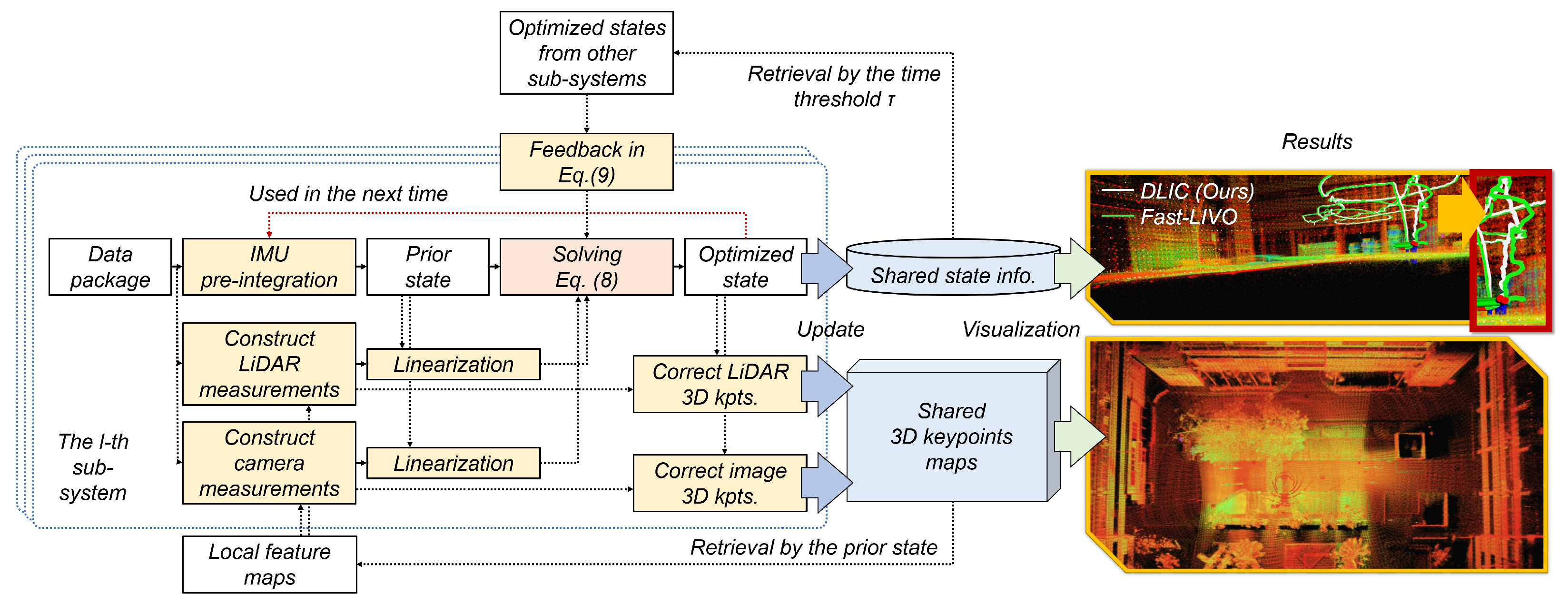
To implement the optimization model in Equation (7), we propose a distributed state estimation method, DLIC, in a multi-LiDAR–IMU–camera system. The DLIC pipeline is provided in Figure 2. The core is to optimize x k l with Equation (8). It mainly has three steps: (i) preparation of Equation (8), (ii) solving Equation (8), and (iii) post-processing.
The first is the preparation of Equation (8). As IMU has a higher publishing rate (≥100 Hz) than other sensors, we follow the previous work [6] to package the LiDAR–IMU–camera data in a time interval. IMU pre-integration is to calculate the prior state x ^ k l and P ^ k from x k 1 l . With x ^ k l , LiDAR measurements contain 3D–3D correspondences between LiDAR scan and the shared LiDAR feature map M lid . They construct ( y i k , H i k ) in Equation (3). Visual measurements denote 2D–3D correspondences from image keypoints to the shared camera feature map M cam (details will be shown in Section 4.4). They construct ( z j k , L j k ) in Equation (3). We retrieve the optimized state from other subsystems with the condition Δ t z l ( τ , τ ) , and construct the feedback constraint via Equation (9).
The second step is to solve Equation (8). With the help of C++ matrix operation library Eigen, x ˜ k l is quickly solved, and x k l is obtained via Equation (6).
The third step is the post-processing. x k l is added into the shared state information with its timestamp. With x k l , we can transform the LiDAR scan into the world coordinate system as S k l and back-projected image keypoints with LiDAR depth (detail is in Section 4.4) into the world coordinate system as V k l . Then, M lid and M cam is updated as:
M lid M lid Down - sample ( S k l ) , M cam M cam V k l
where Down - sample ( · ) is a downsampling operation with voxel resolution of 0.1 m. With the shared feature maps, correspondences of 3D–3D and 2D–3D are stable and precise, ensuring an accurate state estimation result. For better understanding, we illustrate Equation (14) with details. M lid Down - sample ( S k l ) means that the LiDAR feature map is enlarged by merging the point cloud S k l measured by the current scan. To avoid the LiDAR feature map being overly large, the common trick is to downsample S k l . M cam V k l means that the camera feature map is merged with the new keypoints V k l . As the number of visual keypoints (nearly 10 2 ) is smaller than the LiDAR points (nearly 10 4 ), it is not essential to downsample V k l .

4.4. Assisted Image-to-Point-Cloud Registration

From the discussions in Section 2.3, the current approach exploits the VIO subsystem to establish the visual measurement. However, this system fails to work if the initialization is not successful or keypoint tracking fails. Also, the VIO sub-system needs a much greater computational burden for the extra state optimization.
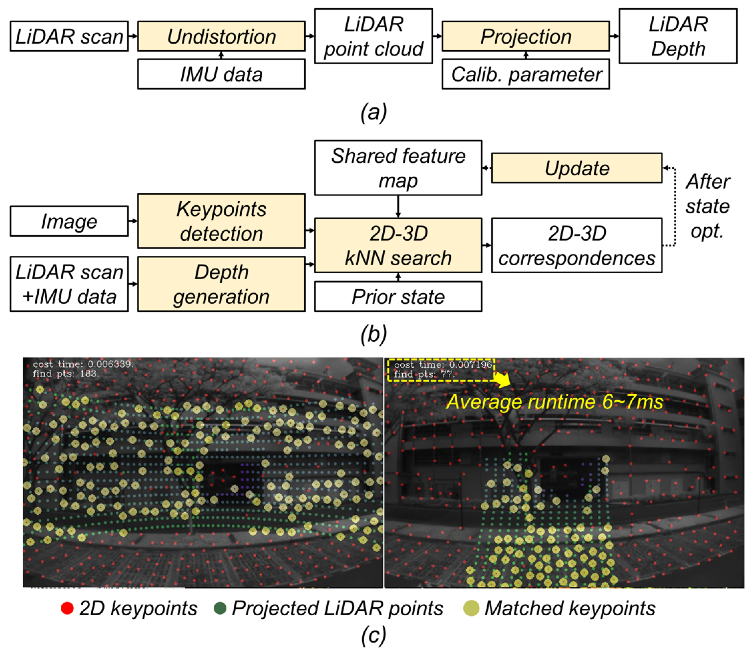
To deal with this issue, we present A-I2P without initialization and extra state optimization. A-I2P needs a shared feature map M cam with the lightweight maintaining cost. A-I2P aims to extract 2D–3D correspondences from image I l and M cam with the aid of P l and IMU data. The procedure is shown in Figure 3. It contains four steps: keypoint detection, depth generation, kNN search, and map update. First, Shi–Tomasi keypoint detector [33] is used to extract { I k } k = 1 K keypoints, as presented as red points in Figure 3c. Second, depth generation aims to project the LiDAR scan, undistorted by IMU data, into the image plane. It obtains the sparse depth, shown as the green points { L s } s = 1 S in Figure 3c. Each pixel L s has depth.
The third step, 2D–3D kNN search, aims to establish 2D–3D correspondences from { I k } k = 1 K , { L s } s = 1 S , M cam . It is a crucial step of A-I2P. For each I k , we search L k { L s } s = 1 S with the nearest distance to I k . We align the depth of I k from L k , when two constraints are satisfied: (i) pixel distance of I k and L k is below τ 2 D where τ 2 D is empirically set as 5 pixels in the actual applications; (ii) gray-scale intensity of I k and L k is below τ I where τ I is empirically set as 24. Keypoints with the aligned depths are marked as { I a } a = 1 A , as presented as the yellow points in Figure 3c. For each I a , we back-project it with its depth to 3D space as 3D point P a . With the initial estimated state x ^ k l , we transform P a from the camera coordinate system to G as P a G . Then, we search a 3D point Q a G M cam with the closest distance to P a G using iKd-Tree [34]. If the distance of P a G and Q a G is below τ 3 D ( τ 3 D is empirically set as 5 cm for optimal performance), pair I a , Q a G is a valid 2D–3D correspondence, and can be used as the visual measurement. As the final estimated state x k l has a slight difference from the initial estimated state x ^ k l , the above correspondence construct scheme with x ^ k l is relatively accurate. After the state optimization, the fourth step is the feature map update, shown in Equation (14). From the above discussion, A-I2P acts like a plug-and-play module. To ensure the correctness of 2D–3D correspondences, it leverages the LiDAR depth to convert 2D–3D correspondence to 3D–3D correspondence, and uses the 3D distance threshold to filter out incorrect 2D–3D correspondences. A-I2P only maintains a feature map with 3D keypoints. It exploits the current LiDAR scan with IMU data, so that A-I2P has a low computational burden. More analysis of DLIC is provided in the Appendix A.

5. Experiments and Discussions

5.1. Dataset Configuration

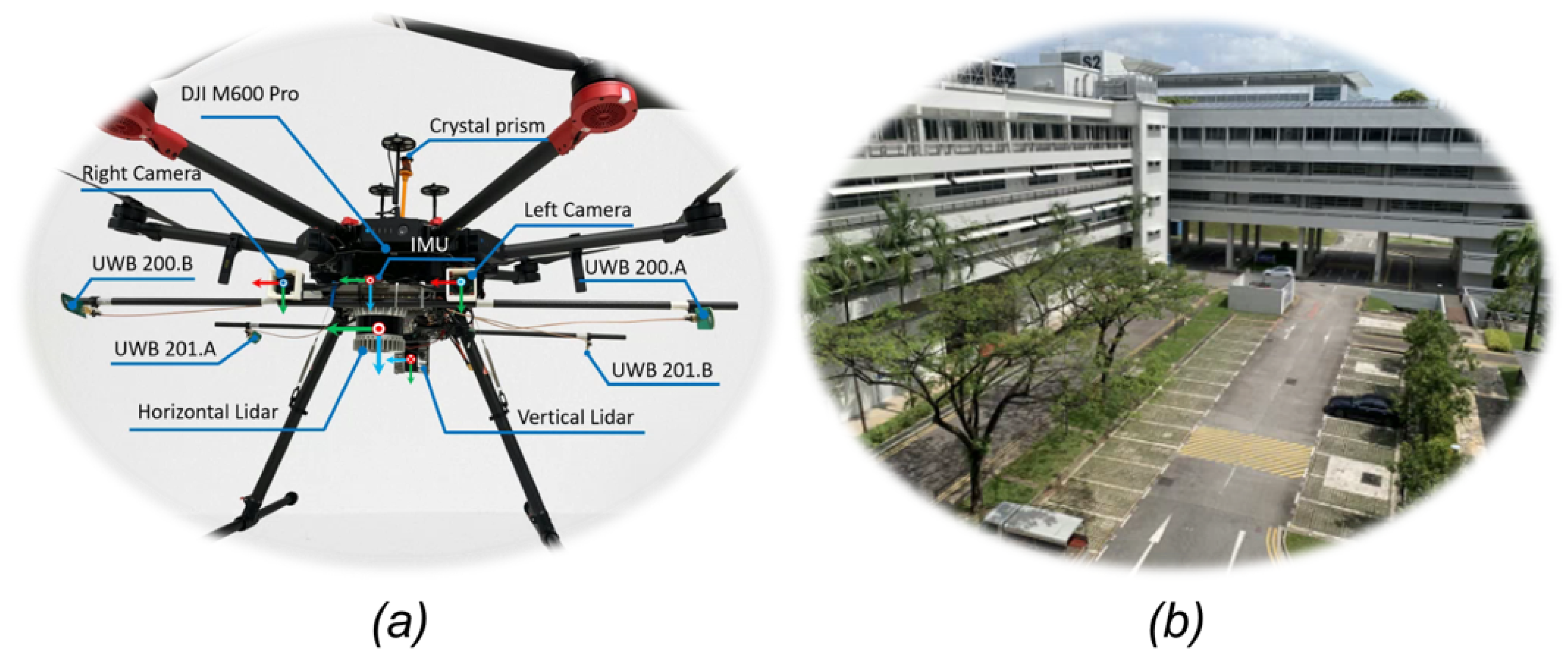
To investigate the performance of multi-sensor-multi-type SLAM methods, we conduct extensive experiments on the public NTU VIRAL [18] dataset, as shown in Figure 4. The NTU VIRAL dataset is selected for three main reasons. First, to the best of our knowledge, it is the first real-world dataset that provides multi-LiDAR–IMU–camera data collected on a single UAV platform equipped with multiple LiDARs, IMUs, and cameras. Second, it includes 18 diverse indoor and outdoor scenes, enabling a comprehensive performance evaluation under varying conditions. Third, this dataset has been widely adopted in previous studies for comparison; however, most existing works utilize only one IMU and conduct evaluations on the first 9 scenes [5,6,11]. In contrast, our experiments demonstrate that by effectively fusing data from multiple sensors, the proposed DLIC achieves superior performance across all 18 scenarios. Notably, we further evaluate DLIC on the remaining 9 scenes for a more complete and rigorous assessment.
Specifically, in the VIRAL dataset, the UAV is equipped with two 16-beam Ouster LiDARs (refresh rate is 10 Hz) and two monocular camera sensors (refresh rate is 10 Hz). Each LiDAR unit integrates an IMU (refresh rate is 100 Hz). The cameras capture 640 × 480 gray-scale images, and their intrinsic parameters are carefully calibrated in advance. Consequently, the UAV constitutes a typical multi-sensor-multi-type system. To obtain the ground truth (GT) position of the UAV, the dataset employs ultra wide band (UWB) technique and a 3D laser tracking system [18]. All sensor data in the NTU VIRAL dataset are recorded using the robot operating system (ROS, an open-source C++ robot platform) and saved as ROS bag files. During the evaluation of state estimation methods, these ROS bags are replayed to reproduce real-time data streams from all sensors. To ensure accurate and synchronized data acquisition, we construct C++ queues that store incoming sensor measurements with their corresponding timestamps.
For the proposed DLIC method, two LiDAR-camera-IMU subsystems are configured ( L = 2 ). The first subsystem consists of the horizontal LiDAR, its associated IMU, and the left camera; the second subsystem includes the vertical LiDAR, its IMU, and the right camera. IMU calibration is performed offline using the parameters provided by the NTU VIRAL dataset, including the extrinsic transformations between the IMU and the LiDAR/camera, as well as intrinsic gyroscope and accelerometer biases. For each subsystem, IMU initialization follows the classical open-source work, FAST-LIO [22]. Data synchronization among LiDAR, IMU, and camera also follows the FAST-LIO, using a first-in-first-out (FIFO) queue strategy. The hyperparameters in the ESIKF are kept consistent with those in Fast-LIVO [6]. To simulate the condition of a commercial UAV onboard system, DLIC is compiled with C++ on an Ubuntu 20.04 Linux system, and tested on a CPU with 8 cores and 8 GB memory.
To evaluate the accuracy of the estimated UAV position, we mainly use RMSE, MAE, SD, and SSE metrics. RMSE and MAE are evaluated in the following manner:
RMSE = 1 U i U T gt , i T i 2 2 , MAE = 1 U i U T gt , i T i 2
where T gt , i and T i are the GT and estimated UAV 3D positions at the i-th time. U is the total time. T gt , i T i 2 2 is the 3D position error at the i-th time. To evaluate the overall trajectory error, RMSE and MAE compute the position error with the different manners. Following the guidance [18], we adjust the temporal difference between the estimated and GT trajectories for the real metric estimation. Metrics SD and SSE are computed from the set { T gt , i T i 2 } i = 1 U . Units of RMSE and MAE are meter. In the following experiments, we utilize EVO (https://github.com/MichaelGrupp/evo (accessed on 24 November 2025)) to compute the above metrics.

5.2. Comparison Results

This experiment investigates the performance of DLIC and existing methods across 18 real-world scenes. The compared approaches contain visual-inertial methods (SVO [28], VINS-Fusion [30]), LiDAR-inertial methods (Fast-LIO [22], D-EKF [13], IGE-LIO [7]), multi-LiDAR method M-LOAM [11], LiDAR-inertial-visual methods (Fast-LIVO [6], R2live [9]). Considering the restricted computational resource of UAVs, only the above methods are included in the comparison, as they have relatively lightweight computational complexity. Since the proposed method can also work in a multi-LiDAR–IMU configuration, we mark it as DLI in this special case. The main quantitative comparison results on the first nine scenes are presented in Table 2. It can be observed that visual-inertial methods [28,30] exhibit unsatisfactory performance compared to other approaches. With the addition of Lidar sensor, the performance improves notably. This contrast is primarily attributed to the high noise and instability of visual measurements in complex environments, which are less reliable than LiDAR data. In particular, the NYA_03 sequence, an indoor scene with weak texture features, further highlights this limitation. Similarly, without IMU assistance, DVL-SLAM [35] suffers from the largest localization errors, as its state estimation is highly sensitive to outliers in visual keypoint matching. These results collectively indicate that leveraging multi-sensor data can significantly enhance overall performance. In contrast, our proposed methods, DLI and DLIC, achieve superior robustness and accuracy by effectively fusing measurements from multiple sensors. This enables them to maintain stable estimation even in noisy or texture-degraded environments, achieving significantly lower RMSE values than competing approaches.
Then, we analyze the performance of state estimation methods with LiDAR-based multi-sensor. From Table 2, the overall RMSE metrics of proposed DLIC and DLI are smaller than current methods, such as R2live [9], R3live [10], M-LOAM [11], IGE-LIO [7], and SR-LIVO [36]. The reasons are illustrated in depth. First, the proposed method utilizes multi-LiDAR, so that it can receive LiDAR measurements with the larger FoVs. Second, DLIC is more robust to IMU measurement noise, for it leverages the multi-IMU to decrease acceleration and angular velocity noises. Third, the proposed method can construct the visual measurement by matching the image and the local feature map. It increases the accuracy and efficiency of visual measurement construction.
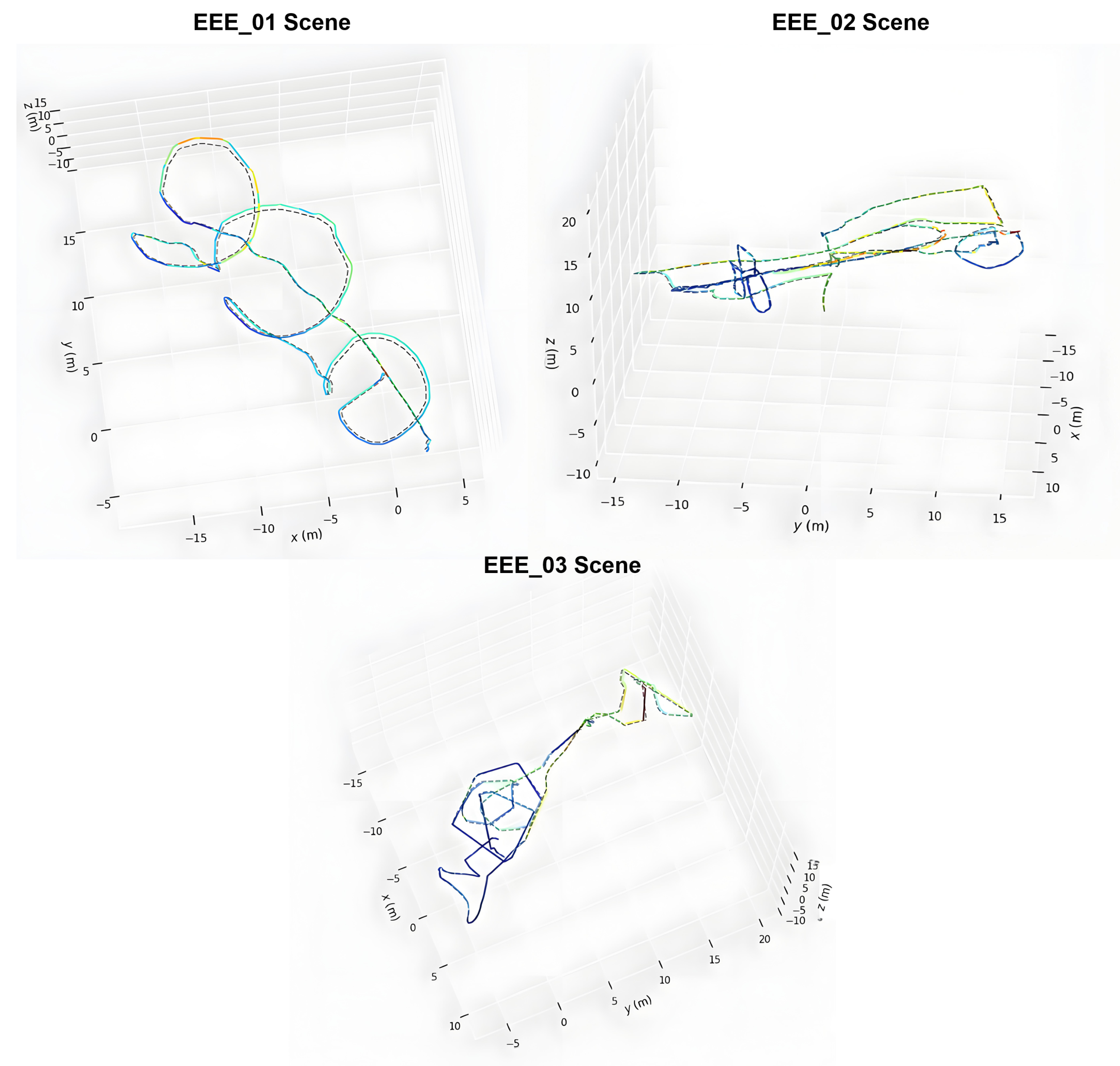
From Table 2, it is observed that some methods, including Fast-LIO [22], Fast-LIVO [6], and D-EKF [13], achieve competitive performance with the proposed DLI and DLIC methods. These methods are further compared where the results are provided in Table 3 and Table 4. In Table 3, we analyze the maximum RMSE and MAE metrics of these methods in the first nine scenes on the NTU VIRAL dataset [18]. Maximum RMSE is an important metric to reflect the stability of state estimation methods. The maximum RMSE of DLIC is always smaller than that of others. It suggests that the proposed distributed state estimation method is robust to multi-sensor measurement noise. MAE is another common metric to evaluate the UAV positional error. MAE of DLI and DLIC is smaller than that of others. Combining the results in Table 2 and Table 3, as well as the visualization of estimated trajectories in Figure 5, the proposed DLIC method has achieved an accurate state estimation result in the various scenes.
In Table 4, we further investigate the generalization ability of these methods in the last nine scenes of the NTU VIRAL dataset [18]. Most methods do not report their performance in these scenarios [6,13,22]. For a fair comparison, we fix the hyper-parameters of all methods and test their generalization ability in unseen scenarios. In the RTP scene, camera images are not saved during the dataset collection, so Fast-LIVO and DLIC cannot work. The results in Table 4 indicate that the proposed DLI and DLIC methods outperform existing methods in the overall metrics (i.e., RMSE, max RMSE, and MAE). The reason is analyzed in-depth. Compared with Fast-LIO and Fast-LIVO, the proposed DLI and DLIC can make use of the measurements from multiple LiDARs, multiple cameras, and multiple IMUs in a distributed estimation manner, thus increasing the robustness to sensor measurement noise. Compared with D-EKF, the proposed method considers the fine-grained multi-IMU measurements. It makes DLI and DLIC more accurate than D-EKF in most scenes. In all, from the results in Table 4, the proposed method achieves a higher generalization ability than existing methods.
Furthermore, to better evaluate the error turbulence caused by multi-sensor-multi-type noise during UAV state estimation, we use other metrics, such as standard deviation (SD) and the sum of squares due to error (SSE), and the result is provided in Table 5. SD and SSE of DLIC are smaller than those of others, for the proposed method makes full use of the multi-sensor-multi-type measurements.
After that, we aim to evaluate the robustness of the proposed DLIC method under different noise levels. Specifically, the sensor noise (i.e., Gaussian random noise with the standard deviation σ LiDAR ) is mainly added into the LiDAR point cloud, which is used to test the stability of multi-sensor-based state estimation methods. σ LiDAR [ 0 , 0.5 ] is divided into five noise levels. RMSE results are provided in Table 6. It is observed that, with the proposed distributed state estimation method, the estimated state is more robust to the sensor noise than other methods.
From the above experiments in the 18 scenes, it is concluded that the proposed DLIC makes full use of the multi-LiDAR–IMU–camera measurements, so that it achieves a more accurate and robust localization performance than current methods in most scenes.

5.3. Visualization Verifications

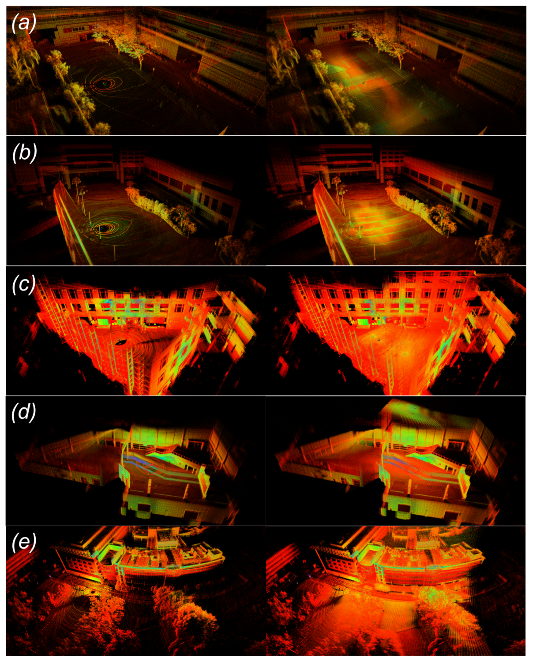
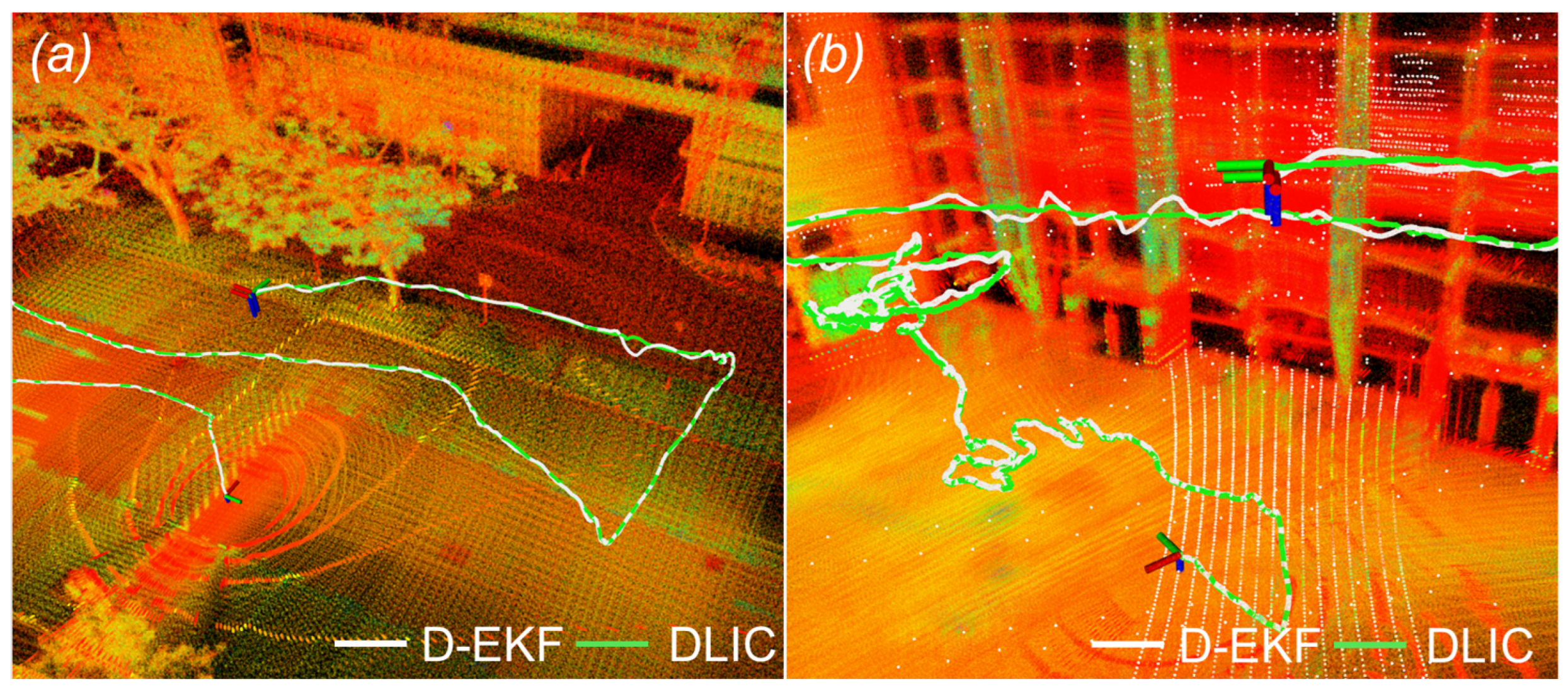
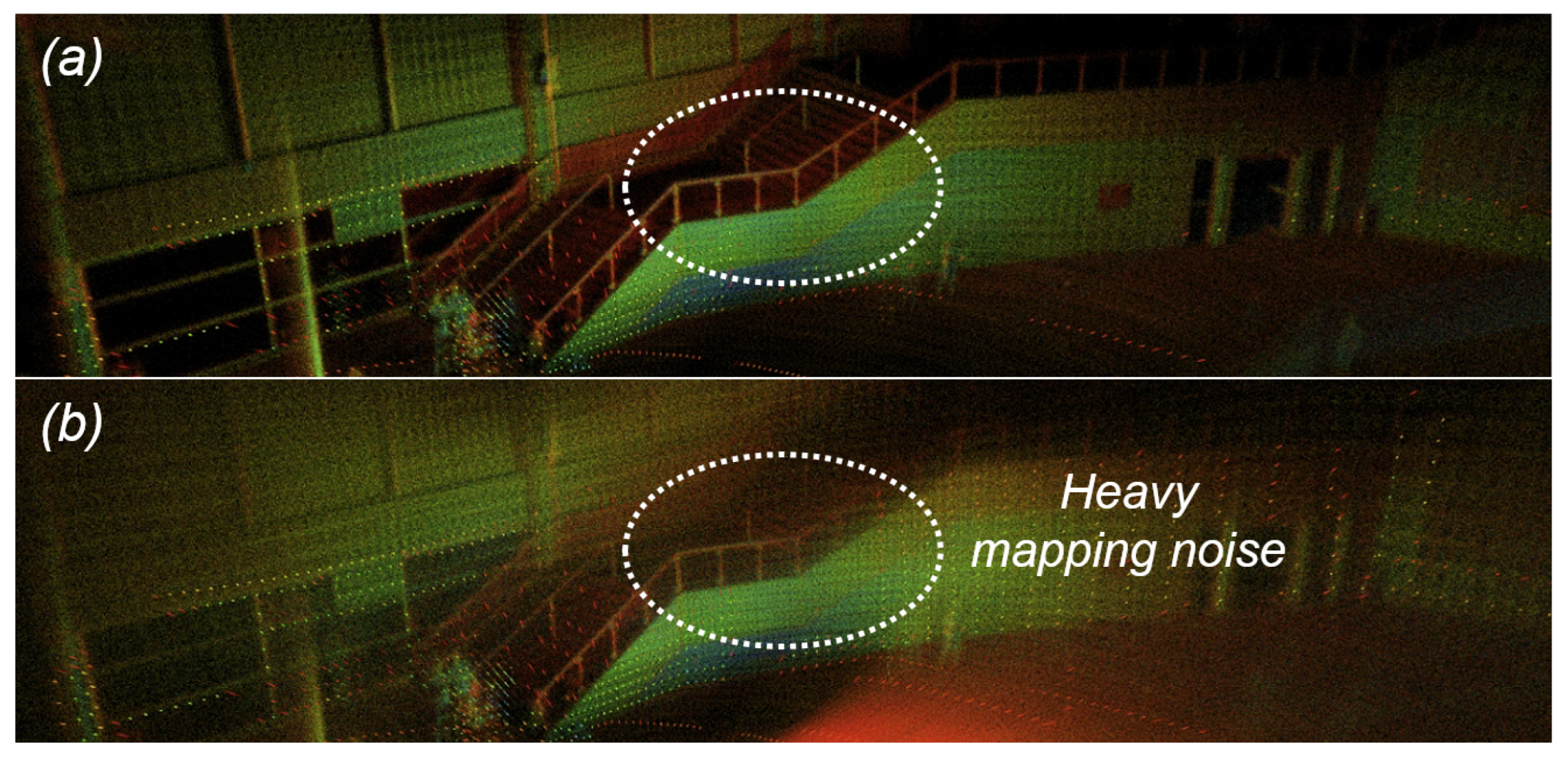
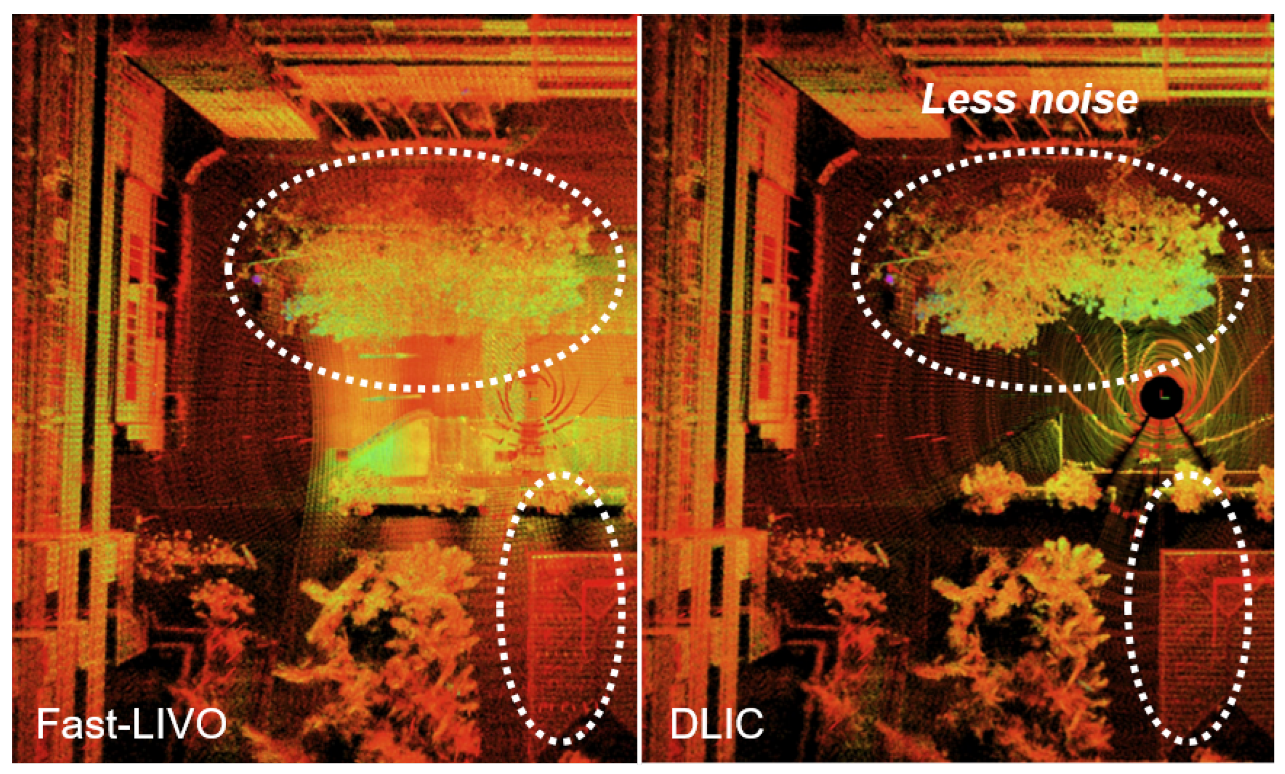
This experiment investigates the reconstruction performance of the proposed method. As the NTU VIRAL dataset [18] does not contain the GT of reconstruction results, we compare the mapping detail as well as visualize the trajectory difference of each approach. As Fast-LIVO [6], DLI, and DLIC have the closest performance in Table 2 and Table 4, these methods are compared in this experiment. The overall mapping results are shown in Figure 6. It is found that the proposed method has a scanning area larger than Fast-LIVO, for the proposed method utilizes the multi-sensor-multi-type information. From Figure 7, it is observed that the trajectory of DLIC is relatively smoother than D-EKF [13], so that DLIC has a smaller RMSE than D-EKF. From Figure 8, the local mapping details show that the reconstruction result by DLIC has less noise than D-EKF [13]. Mapping results of Fast-LIVO [6] and DLIC are provided in Figure 9. The reason why the left image is more blurred than the right one is that the point cloud reconstructed by Fast-LIVO has much greater noise than the proposed method. It indicates that the UAV trajectory estimated by the proposed DLIC method is more accurate than Fast-LIVO. After discussing the mapping results, it is concluded that the proposed DLIC method uses the multi-LiDAR–IMU–camera measurements effectively to obtain the fine-grained 3D mapping results.

5.4. Ablation Studies

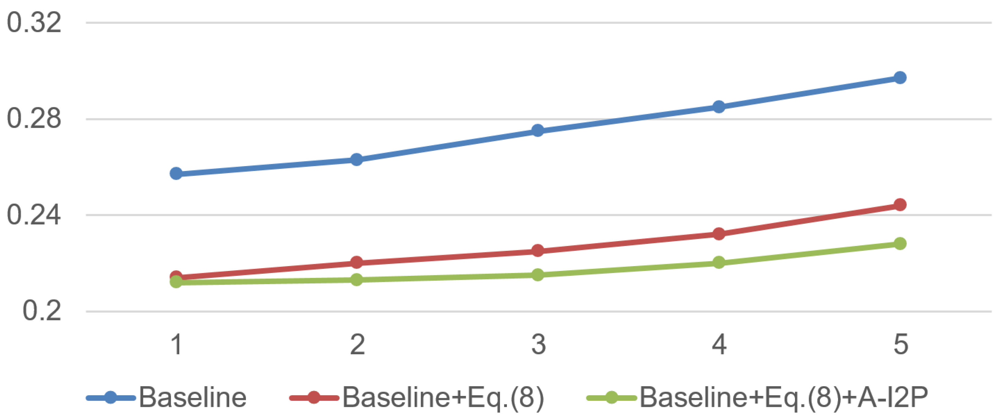
This experiment investigates the performance of each module inside DLIC, with the result provided in Table 7. Baseline means Fast-LIO [22]. Baseline-1 or Baseline-2 means the usage of the horizontal or vertical LiDAR. In the outdoor scene, the horizontal LiDAR sensor has a wide FoV, so that Baseline-1 is more accurate than Baseline-2. Baseline+A-I2P is to add visual measurements in the ESIKF framework. With the usage of A-I2P, the localization accuracy of Baseline-1 and 2 is enhanced, because the 2D–3D correspondences can decrease the negative impact of the noisy 3D–3D correspondences in state estimation. On the other hand, it is found that DLIC also improves the performance of Baseline-1, for it makes use of the observations from Baseline-1 and 2. With the usage of Equation (9) and the A-I2P module, the proposed DLIC has achieved a significant improvement over Baseline-1. In all, the experiment demonstrates that the proposed modules are effective for multi-sensor-multi-type-based SLAM.
To further investigate the robustness of the methods in Table 7, we follow the experimental setting in Table 6 and conduct the noise experiments in Figure 10. With the proposed A-I2P and distributed state estimation model in Equation (8), the proposed method is more robust to sensor noise.
Further, we conduct an experiment to investigate the hyper-parameters τ 2 D , τ I , and τ 3 D of A-I2P on the performance of Baseline+A-I2P. The results are presented in Table 8. τ 2 D [ 1 , 9 ] , τ I [ 6 , 30 ] , τ 3 D [ 2.5 , 12.5 ] . At first, we check τ 2 D , while τ I and τ 3 D are set to default values of 6 and 2.5 cm, respectively. If τ 2 D 5 , RMSE begins to increase, for the large 2D search region causes the inaccuracy of keypoint depth. τ 2 D = 5 has the best RMSE. Then, we fix τ 2 D = 5 and check τ I , while τ 3 D is at the default value. When τ I 30 , the alignment error of LiDAR point and keypoint is increasing, causing the large RMSE error. τ I = 30 is optimal. After that, we fix τ 2 D and τ I , and then study τ 3 D . If τ 3 D is set too large, 3D–3D correspondence searched by kNN is not accurate, causing inaccuracy of mapping. Thus, τ 2 D = 5 , τ I = 24 , τ 3 D = 5.0 cm are the best hyper-parameters in A-I2P.
Moreover, we conduct the runtime analysis, and the result is provided in Table 9. Baseline is Fast-LIO [22]. Compared with Fast-LIO [22], the additional cost of DLIC is mainly the updating of the sharing feature map. Due to the multi-threading technique, solving Equation (8) does not need double the runtime, so that DLI has the closest runtime to Fast-LIO [22]. As A-I2P is an efficient module, the runtime of DLIC is ≈25 ms. Although the state-of-the-art D-EKF method [16] is faster than the proposed methods, it does not fully use the multi-LiDAR–IMU–camera sensor data, so that its state estimation accuracy is less then DLIC. The core of DLIC is the distributed state estimation in Equation (7) and A-I2P. From Table 9, it is found that the Equation (7) costs nearly 1.24 ms and A-I2P costs nearly 5.99 ms. This means that the proposed method is efficient in the actual applications.
We also analyze the peak memory usage of the proposed method. In this test, the memory of visualization from ROS RVIZ is not included. In an SLAM system, it is noted that the memory usage is related to the mapping area, because the feature map storage is the dominant factor in memory usage. In the EEE_03 scene, the result of peak memory usage is presented in Table 10. For a fair comparison, Fast-LIVO denotes the combination of two groups of LiDAR–camera–inertial system, in the meantime, as DLIC does. As DLIC can filter the overlapped 3D keypoints during the updating of iKd-Tree [34], DLIC saves nearly 0.5 GB of memory compared to Fast-LIVO . Further, we also investigate the effect of the voxel size of the proposed method and the results are shown in Table 11. The default map voxel size is 0.050 m in the experiments. We test the performance of DLIC if the voxel size is 0.025 m and 0.100 m. When the voxel size is decreased to 0.025 m, the mapping resolution is enlarged with the overlarge CPU memory cost. If the voxel size is enlarged as 0.100 m, most mapping details are lost, such that the RMSE error is larger than 0.35 m. Thus, it is recommended to set the proper voxel size in the actual applications. From the above experiments, DLIC is a real-time state estimation method with light memory usage.

5.5. Limitations and Future Works

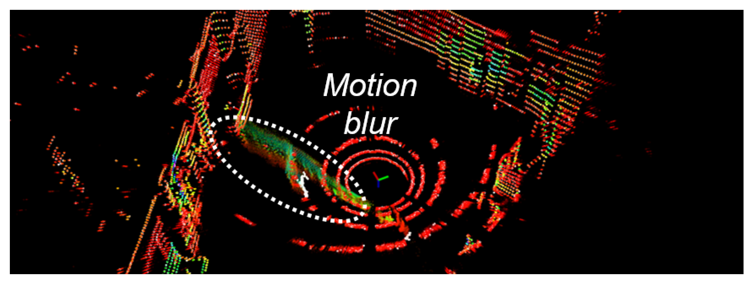
From the above method comparisons, visualization analysis, and ablation studies, it is found that DLIC has made a certain amount of progress in the various scenarios. However, there are still some potential improvements for DLIC. First, since DLIC is not equipped with a loop closure detection and optimization module, this issue may limit the performance of DLIC in long-range state estimation. We will design a specific loop closure module for the multi-sensor-multi-type system. Second, moving objects have a certain negative impact (i.e., motion blur) in the proposed method, as shown in Figure 11. We will address this issue in future work. Third, although our current fusion strategy demonstrates reasonable performance, it remains handcrafted. Exploring deep learning or AI-driven adaptive fusion techniques may better handle complex environments and further enhance both robustness and efficiency. We will pursue this direction in future work. Fourth, as there are few datasets that support state estimation on multi-sensor-multi-type-based systems, it is essential to establish a simulation environment on ROS to collect the multi-sensor-multi-type measurements in future work. It will greatly benefit the algorithm development of state estimation on multi-sensor-multi-type-based systems.

6. Conclusions

We propose an efficient and accurate distributed state estimation method, DLIC, which effectively fuses data from multi-LiDAR–IMU–camera sensors and estimates the UAV’s state. At first, we develop a theoretical state estimation model. It decomposes the original complex estimation problem into multiple low-complexity optimization sub-problems, which can be easily solved with a modern embedded system with a multi-core CPU. The proposed distributed state estimation model has a feedback function that serves as a bridge to interact with state estimation results from all subsystems. After that, we implement the above theoretical model and propose a method, DLIC, for a system with multi-LiDAR–IMU–camera sensors. In DLIC, we propose an A-I2P module to construct accurate 2D–3D correspondences with the aid of LiDAR depth. Extensive experiments on the public real-world NTU VIRAL dataset demonstrate the effectiveness of the proposed DLIC method. Thus, we believe that the proposed DLIC method benefits the development of multi-sensor autonomous systems.

Author Contributions

Conceptualization, J.D. and P.A.; methodology, J.D. and P.A.; software, T.M.; validation, J.D.; formal analysis, K.Y. and B.F.; investigation, T.M.; resources, P.A.; data curation, J.D.; writing—original draft preparation, J.D. and P.A.; writing—review and editing, J.M.; visualization, K.Y. and B.F.; supervision, P.A. and T.M.; project administration, J.M.; funding acquisition, P.A. All authors have read and agreed to the published version of the manuscript.

Funding

This work is partially supported by National Key R&D Program of China (Grant ID: 2024YFC3015303), National Science Foundation of China (Grand ID: 62502171, 62201536), National Key Laboratory of Electromagnetic Energy (Grant ID: 6142217242040101), and China Postdoctoral Science Foundation (Grand ID: 2024M761014).

Data Availability Statement

The NTU VIRAL dataset can be found at https://ntu-aris.github.io/ntu_viral_dataset/ (accessed on 24 November 2025).

Conflicts of Interest

The authors declare no conflicts of interest.

Abbreviations

The following abbreviations are used in this manuscript:
UAVUnmanned aerial vehicle
FoVField of view
RGBRed, green, blue
LiDARLight detection and ranging
IMUInertial measurement unit
CPUCentral processing unit
I2PImage-to-point cloud
LIVOLiDAR-inertial-visual odometry
LIOLiDAR-inertial odometry
ESIKFError state iterative Kalman filter
SDStandard deviation
SSESum of squared errors
RMSERoot mean square error
MAEMean absolute error
SLAMSimultaneous localization and mapping
UWBUltra wide band
GTGround truth
kNNk-nearest neighbor
MAPMaximum a posterior
EKFExtended Kalman filter
GPSGlobal positioning system

Appendix A. Further Discussion of DLIC

The effectiveness of multi-LiDAR–IMU-based state estimation methods has been analyzed in previous work [13]. In this appendix, we focus on discussing the effectiveness of the proposed multi-LiDAR–IMU–Camera-based state estimation method, DLIC.
First, measurements from multiple IMUs can alleviate the white noise inherent in a single IMU. If the intrinsic parameters (i.e., accelerometer and gyroscope biases of each IMU) and extrinsic parameters (i.e., rigid transformations between IMUs) are accurately calibrated, the combined measurements of multiple IMUs can approximate those of a single IMU with a higher sampling frequency, thereby reducing the negative impact of noise in IMU pre-integration [19]. Consequently, using multiple IMUs improves the accuracy of the 6-DoF pose estimated from IMU data.
Second, employing multiple LiDARs and cameras increases the number of 2D–3D and 3D–3D correspondences, significantly mitigating the negative effects of correspondence noise on state estimation. In DLIC, camera measurements are constructed through I2P registration. Multiple LiDARs and cameras enhance the field of view (FoV) of perception and enlarge the FoV overlap between LiDARs and cameras. Furthermore, multiple LiDARs alleviate the sparsity of point clouds captured by a single LiDAR. These factors collectively improve correspondence accuracy, ensuring the construction of reliable camera and LiDAR measurements.
Based on the above discussions, a general multi-sensor-multi-type system can effectively suppress noise in each sensor type. As a result, it achieves more accurate state estimation performance compared with other multi-sensor-based methods, as shown in Table 2, Table 3 and Table 4.

References

  1. Cui, J.; Niu, J.; He, Y.; Liu, D.; Ouyang, Z. ACLC: Automatic Calibration for Nonrepetitive Scanning LiDAR-Camera System Based on Point Cloud Noise Optimization. IEEE Trans. Instrum. Meas. 2024, 73, 5001614. [Google Scholar] [CrossRef]
  2. Zhou, Y.; Li, J.; Ou, C.; Yan, D.; Zhang, H.; Xue, X. Open-Vocabulary Object Detection in UAV Imagery: A Review and Future Perspectives. Drones 2025, 9, 557. [Google Scholar] [CrossRef]
  3. Lv, M.; Zhang, B.; Duan, H.; Shi, Y.; Zhou, C. Unmanned Aerial Vehicles Formation Control and Safety Guarantee; Springer Nature: Singapore, 2025. [Google Scholar]
  4. Li, K.; Bu, S.; Li, J.; Xia, Z.; Wang, J.; Li, X. Distributed Relative Pose Estimation for Multi-UAV Systems Based on Inertial Navigation and Data Link Fusion. Drones 2025, 9, 405. [Google Scholar] [CrossRef]
  5. Lv, J.; Lang, X.; Xu, J.; Wang, M.; Liu, Y.; Zuo, X. Continuous-Time Fixed-Lag Smoothing for LiDAR-Inertial-Camera SLAM. IEEE/ASME Trans. Mechatronics 2023, 28, 2259–2270. [Google Scholar] [CrossRef]
  6. Zheng, C.; Zhu, Q.; Xu, W.; Liu, X.; Guo, Q.; Zhang, F. FAST-LIVO: Fast and Tightly-coupled Sparse-Direct LiDAR-Inertial-Visual Odometry. In Proceedings of the IEEE/RSJ International Conference on Intelligent Robots and Systems, Kyoto, Japan, 23–27 October 2022; pp. 4003–4009. [Google Scholar]
  7. Chen, Z.; Zhu, H.; Yu, B.; Jiang, C.; Hua, C.; Fu, X.; Kuang, X. IGE-LIO: Intensity Gradient Enhanced Tightly Coupled LiDAR-Inertial Odometry. IEEE Trans. Instrum. Meas. 2024, 73, 8506411. [Google Scholar] [CrossRef]
  8. Zhao, X.; Wen, C.; Prakhya, S.M.; Yin, H.; Zhou, R.; Sun, Y.; Xu, J.; Bai, H.; Wang, Y. Multimodal Features and Accurate Place Recognition with Robust Optimization for Lidar-Visual-Inertial SLAM. IEEE Trans. Instrum. Meas. 2024, 73, 5033916. [Google Scholar] [CrossRef]
  9. Lin, J.; Zheng, C.; Xu, W.; Zhang, F. R2LIVE: A Robust, Real-Time, LiDAR-Inertial-Visual Tightly-Coupled State Estimator and Mapping. IEEE Robot. Autom. Lett. 2021, 6, 7469–7476. [Google Scholar] [CrossRef]
  10. Lin, J.; Zhang, F. R3LIVE: A Robust, Real-time, RGB-colored, LiDAR-Inertial-Visual tightly-coupled state Estimation and mapping package. In Proceedings of the IEEE International Conference on Robotics and Automation, Philadelphia, PA, USA, 23–27 May 2022; pp. 10672–10678. [Google Scholar]
  11. Jiao, J.; Ye, H.; Zhu, Y.; Liu, M. Robust Odometry and Mapping for Multi-LiDAR Systems with Online Extrinsic Calibration. IEEE Trans. Robot. 2022, 38, 351–371. [Google Scholar] [CrossRef]
  12. Wang, Y.; Song, W.; Lou, Y.; Huang, F.; Tu, Z.; Zhang, S. Simultaneous Localization of Rail Vehicles and Mapping of Environment with Multiple LiDARs. IEEE Robot. Autom. Lett. 2022, 7, 8186–8193. [Google Scholar] [CrossRef]
  13. Lin, J.; Liu, X.; Zhang, F. A decentralized framework for simultaneous calibration, localization and mapping with multiple LiDARs. In Proceedings of the IEEE/RSJ International Conference on Intelligent Robots and Systems, Las Vegas, NV, USA, 24 October 2020–24 January 2021; pp. 4870–4877. [Google Scholar]
  14. Nguyen, T.; Duberg, D.; Jensfelt, P.; Yuan, S.; Xie, L. SLICT: Multi-Input Multi-Scale Surfel-Based Lidar-Inertial Continuous-Time Odometry and Mapping. IEEE Robot. Autom. Lett. 2023, 8, 2102–2109. [Google Scholar] [CrossRef]
  15. Nguyen, T.; Yuan, S.; Cao, M.; Lyu, Y.; Nguyen, T.H.; Xie, L. MILIOM: Tightly Coupled Multi-Input Lidar-Inertia Odometry and Mapping. IEEE Robot. Autom. Lett. 2021, 6, 5573–5580. [Google Scholar] [CrossRef]
  16. Wang, Z.; Zhang, L.; Shen, Y.; Zhou, Y. D-LIOM: Tightly-Coupled Direct LiDAR-Inertial Odometry and Mapping. IEEE Trans. Multim. 2023, 25, 3905–3920. [Google Scholar] [CrossRef]
  17. Jung, M.; Jung, S.; Kim, A. Asynchronous Multiple LiDAR-Inertial Odometry Using Point-Wise Inter-LiDAR Uncertainty Propagation. IEEE Robot. Autom. Lett. 2023, 8, 4211–4218. [Google Scholar] [CrossRef]
  18. Nguyen, T.; Yuan, S.; Cao, M.; Lyu, Y.; Nguyen, T.H.; Xie, L. NTU VIRAL: A visual-inertial-ranging-lidar dataset, from an aerial vehicle viewpoint. Int. J. Robot. Res. 2022, 41, 270–280. [Google Scholar] [CrossRef]
  19. Forster, C.; Carlone, L.; Dellaert, F.; Scaramuzza, D. On-Manifold Preintegration for Real-Time Visual-Inertial Odometry. IEEE Trans. Robot. 2017, 33, 1–21. [Google Scholar] [CrossRef]
  20. Shan, T.; Englot, B.J.; Meyers, D.; Wang, W.; Ratti, C.; Rus, D. LIO-SAM: Tightly-coupled Lidar Inertial Odometry via Smoothing and Mapping. In Proceedings of the IEEE/RSJ International Conference on Intelligent Robots and Systems, Las Vegas, NV, USA, 24 October 2020–24 January 2021; pp. 5135–5142. [Google Scholar]
  21. Shan, T.; Englot, B.J.; Ratti, C.; Rus, D. LVI-SAM: Tightly-coupled Lidar-Visual-Inertial Odometry via Smoothing and Mapping. In Proceedings of the IEEE International Conference on Robotics and Automation, Xi’an, China, 30 May–5 June 2021; pp. 5692–5698. [Google Scholar]
  22. Xu, W.; Zhang, F. FAST-LIO: A Fast, Robust LiDAR-Inertial Odometry Package by Tightly-Coupled Iterated Kalman Filter. IEEE Robot. Autom. Lett. 2021, 6, 3317–3324. [Google Scholar] [CrossRef]
  23. Zhang, J.; Singh, S. Low-drift and real-time lidar odometry and mapping. Auton. Robot. 2017, 41, 401–416. [Google Scholar] [CrossRef]
  24. Shan, T.; Englot, B.J. LeGO-LOAM: Lightweight and Ground-Optimized Lidar Odometry and Mapping on Variable Terrain. In Proceedings of the IEEE/RSJ International Conference on Intelligent Robots and Systems, Madrid, Spain, 1–5 October 2018; pp. 4758–4765. [Google Scholar]
  25. Qin, C.; Ye, H.; Pranata, C.E.; Han, J.; Zhang, S.; Liu, M. LINS: A Lidar-Inertial State Estimator for Robust and Efficient Navigation. In Proceedings of the IEEE International Conference on Robotics and Automation, Paris, France, 31 May–31 August 2020; pp. 8899–8906. [Google Scholar]
  26. Ye, H.; Chen, Y.; Liu, M. Tightly Coupled 3D Lidar Inertial Odometry and Mapping. In Proceedings of the IEEE International Conference on Robotics and Automation, Montreal, QC, Canada, 20–24 May 2019; pp. 3144–3150. [Google Scholar]
  27. Li, T.; Pei, L.; Xiang, Y.; Zuo, X.; Yu, W.; Truong, T. P3-LINS: Tightly Coupled PPP-GNSS/INS/LiDAR Navigation System with Effective Initialization. IEEE Trans. Instrum. Meas. 2023, 72, 8501813. [Google Scholar] [CrossRef]
  28. Forster, C.; Zhang, Z.; Gassner, M.; Werlberger, M.; Scaramuzza, D. SVO: Semidirect Visual Odometry for Monocular and Multicamera Systems. IEEE Trans. Robot. 2017, 33, 249–265. [Google Scholar] [CrossRef]
  29. Lin, J.; Zhang, F. R3LIVE++: A Robust, Real-time, Radiance reconstruction package with a tightly-coupled LiDAR-Inertial-Visual state Estimator. IEEE Trans. Pattern Anal. Mach. Intell. 2024, 46, 11168–11185. [Google Scholar] [CrossRef]
  30. Qin, T.; Li, P.; Shen, S. VINS-Mono: A Robust and Versatile Monocular Visual-Inertial State Estimator. IEEE Trans. Robot. 2018, 34, 1004–1020. [Google Scholar] [CrossRef]
  31. Furgale, P.T.; Tong, C.H.; Barfoot, T.D.; Sibley, G. Continuous-time batch trajectory estimation using temporal basis functions. Int. J. Robot. Res. 2015, 34, 1688–1710. [Google Scholar] [CrossRef]
  32. Duberg, D.; Jensfelt, P. UFOMap: An Efficient Probabilistic 3D Mapping Framework That Embraces the Unknown. IEEE Robot. Autom. Lett. 2020, 5, 6411–6418. [Google Scholar] [CrossRef]
  33. Shi, J.; Tomasi, C. Good features to track. In Proceedings of the IEEE Conference on Computer Vision and Pattern Recognition, Seattle, WA, USA, 21–23 June 1994; pp. 593–600. [Google Scholar]
  34. Cai, Y.; Xu, W.; Zhang, F. ikd-Tree: An Incremental K-D Tree for Robotic Applications. arXiv 2021, arXiv:2102.10808. [Google Scholar]
  35. Shin, Y.; Park, Y.S.; Kim, A. DVL-SLAM: Sparse depth enhanced direct visual-LiDAR SLAM. Auton. Robot. 2020, 44, 115–130. [Google Scholar] [CrossRef]
  36. Yuan, Z.; Deng, J.; Ming, R.; Lang, F.; Yang, X. SR-LIVO: LiDAR-Inertial-Visual Odometry and Mapping with Sweep Reconstruction. IEEE Robot. Autom. Lett. 2024, 9, 5110–5117. [Google Scholar] [CrossRef]
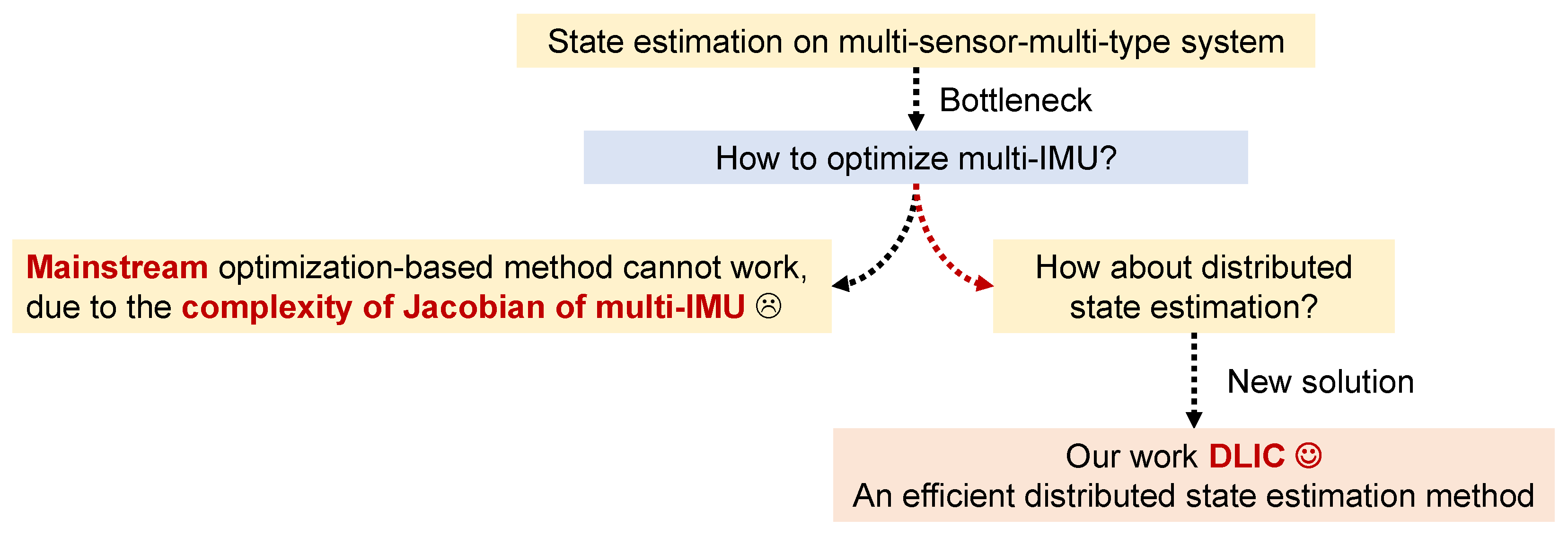
Figure 1. Illustration of the bottleneck of current methods and the new solution proposed in this paper.
Drones 09 00823 g001
Figure 2. DLIC pipeline. The core step is to optimize the state via Equation (8). The inputs of Equation (8) are the prior state, LiDAR measurements, visual measurements, and feedback, respectively. The prior state is estimated with IMU pre-integration. LiDAR and visual measurements are constructed with local feature maps. After optimization, DLIC maintains the shared state information and 3D keypoint maps, which are crucial to construct LiDAR, visual measurements, and feedback for the next time. Compared with Fast-LIVO [6], DLIC can obtain a stable and accurate flight trajectory, as well as a high-quality reconstruction scene.
Drones 09 00823 g002
Figure 3. Procedure of A-I2P. (a) Depth generation is to project the undistorted LiDAR point cloud into the image plane as the LiDAR depth. (b) A-I2P contains four steps, including keypoint detection, depth generation, kNN search, and update. (c) Visualization of A-I2P. A-I2P is very fast in practical applications.
Drones 09 00823 g003
Figure 4. Details of the NTU VIRAL dataset [18]. (a) UAV equipped with two LiDARs, two cameras, and multiple IMUs. (b) Experiment sites are used to evaluate the proposed state estimation method.
Drones 09 00823 g004
Figure 5. Visualization of the estimated trajectories of UAV in EEE_01, EEE_02, and EEE_03 scenes on the NTU VIRAL dataset [18]. In most cases, the positions estimated by DLIC have relatively small errors. Black dotted line is the GT trajectory while the color line is the trajectory computed by our method.
Drones 09 00823 g005
Figure 6. Visualization of Fast-LIVO (Up) [6] and proposed DLIC (Down) in the different scenarios from (ae). Pseudo color reflects the value of LiDAR intensity. DLIC utilizes the multi-sensor with large FoVs, so that it reconstructs a 3D scene more completely than Fast-LIVO.
Drones 09 00823 g006
Figure 7. Trajectory visualization of the proposed DLIC and D-EKF [13]. (a) EEE scene. (b) TNP scene. When the UAV moves fast, the trajectory of D-EKF tends to fluctuate, while the trajectory of DLIC is still smooth and accurate.
Drones 09 00823 g007
Figure 8. Mapping details of the different methods. (a) DLIC. (b) D-EKF [13]. The proposed method reconstructs the buildings with less noise.
Drones 09 00823 g008
Figure 9. Mapping results of Fast-LIVO (left) and DLIC (right). Compared with Fast-LIVO, DLIC achieves more accurate state estimation results, so that it reconstructs the 3D outdoor scene with less noise than Fast-LIVO.
Drones 09 00823 g009
Figure 10. RMSE of the different methods on EEE_03 scene with the various sensor noise levels (from 1 to 5). DLI is the baseline + Equation (8) and DLIC is the baseline + Equation (8) + A-I2P.
Drones 09 00823 g010
Figure 11. Moving objects have a certain negative impact (i.e., motion blur) in the proposed method. We will address this issue in future work.
Drones 09 00823 g011
Table 1. Main symbols notation.
SymbolMeaning
x , x ^ , x ˜ State of ground truth, estimation, residual error
I , W , A , k subscript: IMU coordinate system, gyroscope, accelerometer, timestamp
p I , v I , ξ I 3D position, velocity, rotation vector
b W , b A , g IMU basis of gyroscope and accelerometer, gravity vector
J k , P ^ k Jacobian, covariance matrix of pre-integration on x ^ k
M l Feature map of the l-th Kalman filter
P l 3D point at the current LiDAR coordinate system
P l G 3D point at the global coordinate system G
I2D pixel coordinate in the image
y i , z j correspondence: LiDAR point, image point
Table 2. RMSE results of the compared methods on the first nine scenes in the NTU VIRAL dataset. L, I, C means the usage of LiDAR, IMU, and camera. L1 and L2 mean the usage of single LiDAR and double LiDAR. Red bold is 1st, and blue bold is 2nd.
RMSE MetricSensor UsageEEE_01EEE_02EEE_03NYA_01NYA_02NYA_03SBS_01SBS_02SBS_03
Fast-LIO [22]L1+I10.5400.2200.2500.2400.2100.2300.2500.2600.240
Fast-LIVO [6]L1+I1+C10.2800.1700.2300.1900.1800.1900.2900.2200.220
DVL-SLAM [35]L1+C12.8801.6503.0802.0901.4501.8201.0802.3102.230
SVO [28]I1+C1FailFail4.1202.2902.9103.3207.840FailFail
VINS-Fusion [30]I1+C10.6080.5060.4940.3970.4240.7870.5080.5640.878
R2Live [9]L1+I1+C10.4500.2100.9700.1900.6300.3100.5600.2400.440
M-LOAM [11]L20.2490.1660.2320.1230.1910.2260.1730.1470.153
D-EKF [13]L2+I20.2690.1640.2200.2290.1780.2070.2080.2200.244
IGE-LIO [7]L1+I10.2090.1970.2170.2310.1950.1940.2070.2190.212
R3Live [10]L1+I1+C11.6900.6400.6300.3500.2300.4000.2700.210
SR-LIVO [36]L1+I1+C10.2100.2300.2200.1800.1900.2000.1200.2200.210
DLI (Our)L2+I20.2560.1520.2110.1960.1660.1830.1850.1810.182
DLIC (Our)L2+I2+C20.2370.1460.2080.1660.1430.1700.1620.1600.173
Table 3. Other metrics of the compared methods on the first nine scenes in the NTU VIRAL dataset. Red bold is 1st, and blue bold is 2nd.
MAX RMSE MetricEEE_01EEE_02EEE_03NYA_01NYA_02NYA_03SBS_01SBS_02SBS_03
Fast-LIO [22]0.6330.7320.6380.6490.4630.5420.6540.5870.513
Fast-LIVO [6]0.5860.6280.5820.6410.4590.4880.5880.5560.492
D-EKF [13]1.0120.6210.4380.5880.4690.6300.7090.4920.504
DLI (Our)0.9730.5410.4110.5200.5450.4660.4390.4350.491
DLIC (Our)0.5190.4070.3640.6080.4430.4550.4200.4150.464
MAE MetricEEE_01EEE_02EEE_03NYA_01NYA_02NYA_03SBS_01SBS_02SBS_03
Fast-LIO [22]0.2770.1520.2310.2100.1910.1970.2310.2540.231
Fast-LIVO [6]0.2480.1360.2190.2150.1840.1750.2610.2010.205
D-EKF [13]0.2520.1410.2080.1900.1610.1810.1980.2070.232
DLI (Our)0.2420.1290.1990.1670.1340.1500.1650.1590.163
DLIC (Our)0.2240.1260.1960.1350.1130.1440.1340.1420.151
Table 4. Results of the compared methods on the last nine scenes in the NTU VIRAL dataset. Red bold is 1st, and blue bold is 2nd.
RMSE MetricRTP_01RTP_02RTP_03TNP_01TNP_02TNP_03SPMS_01SPMS_02SPMS_03
Fast-LIO [22]0.4020.2400.6360.1380.1590.1740.6352.2161.595
Fast-LIVO [6]0.1140.1070.1950.9751.2112.043
D-EKF [13]0.2980.1650.6330.0960.1090.1780.3632.0471.505
DLI (Our)0.2160.1570.5720.0950.1040.1440.3011.8980.684
DLIC (Our)0.0880.0980.1110.2851.1981.328
MAX RMSE MetricRTP_01RTP_02RTP_03TNP_01TNP_02TNP_03SPMS_01SPMS_02SPMS_03
Fast-LIO [22]1.6670.7411.9910.3920.3280.4224.3767.0465.250
Fast-LIVO [6]0.3040.4210.3772.1654.6074.631
D-EKF [13]1.9020.4982.0030.3320.4850.6041.9578.0555.695
DLI (Our)0.7820.3391.9760.3100.4010.4211.1125.4323.305
DLIC (Our)0.2510.2950.5111.0624.1613.574
MAE MetricRTP_01RTP_02RTP_03TNP_01TNP_02TNP_03SPMS_01SPMS_02SPMS_03
Fast-LIO [22]0.3180.1960.5780.1260.1480.1430.4891.6411.405
Fast-LIVO [6]0.0960.0970.1810.8970.9891.779
D-EKF [13]0.2870.1500.5630.0780.1210.1520.2871.5541.318
DLI (Our)0.2520.1430.5170.0750.0930.1020.2601.3880.464
DLIC (Our)0.0680.0790.0760.2510.9471.240
Table 5. State error turbulence evaluation of current state estimation methods on EEE_03 scene. Red bold is 1st.
MetricsFast-LIO [22]Fast-LIVO [6]D-EKF [13]DLIC
SD0.1010.0710.0680.062
SSE12.33810.21210.0759.241
Table 6. Robustness evaluation of the current state estimation methods on EEE_01 scene. Red bold is 1st.
Noise LevelsFast-LIO [22]Fast-LIVO [6]D-EKF [13]DLIC
00.5400.2800.2690.237
10.5480.2850.2720.241
20.5520.2880.2780.242
30.5630.2910.2800.245
40.5780.2930.2840.247
50.5830.2980.2900.256
Table 7. Ablation study of DLIC on EEE_03 scene. Red bold is 1st.
MethodRMSE MetricMAE Metric
Baseline-10.2500.210
Baseline-20.2840.233
Baseline-1+A-I2P0.2190.207
Baseline-2+A-I2P0.2310.211
Baseline + Equation (8) (DLI)0.2110.199
Baseline + Equation (8) + A-I2P (DLIC)0.2080.196
Table 8. Ablation study of hyper-parameters of A-I2P on EEE_03 scene. Red bold is 1st.
τ 2 D 13579
RMSE0.2480.2450.2440.2510.254
τ I 612182430
RMSE0.2440.2410.2340.2210.238
τ 3 D 2.55.07.510.012.5
RMSE0.2210.2190.2280.2310.234
Table 9. Runtime analysis of DLIC on EEE_03 scene.
MethodAverage Runtime per Loop
D-EKF18.89 ms
Baseline18.32 ms
Baseline + A-I2P24.31 ms
Baseline + Equation (9) (DLI)19.56 ms
Baseline + Equation (9) + A-I2P (DLIC)25.86 ms
Table 10. Peak memory usage of DLIC on EEE_03 scene. denotes different sensor configurations.
MethodSensor UsagePeak Memory Usage
Fast-LIVO [6]L1+C1+I11821 MB
Fast-LIVO [6]L2+C2+I23277 MB
DLICL2+C2+I22741 MB
Table 11. RMSE and peak memory usage of DLIC on EEE_03 scene under different voxel size.
Voxel Size0.025 m0.050 m0.100 m
RMSE0.201 m0.208 m0.352 m
Peak memory usage8421 MB2741 MB723 MB
Disclaimer/Publisher’s Note: The statements, opinions and data contained in all publications are solely those of the individual author(s) and contributor(s) and not of MDPI and/or the editor(s). MDPI and/or the editor(s) disclaim responsibility for any injury to people or property resulting from any ideas, methods, instructions or products referred to in the content.