A Mission-Oriented Autonomous Missile Evasion Maneuver Decision-Making Method for Unmanned Aerial Vehicle

Highlights

What are the main findings?

• Agents trained using the algorithm proposed in this paper are deployed to operate two distinct unmanned aerial vehicle (UAV) platforms in air-to-air game scenarios. Under head-on and parallel initial configurations, the evasion success rates of the UAVs are comparable. In the tail-chase scenario, the evasion success rates reach 90% and 85%, respectively. This demonstrates that the decision-making model constructed in this paper exhibits a degree of platform transferability.
• To enhance the decision model’s applicability across diverse scenarios, a training mechanism with randomized initial scenarios is designed. When the missile initially positions itself ahead, behind, or to the side of the UAV, the UAV’s missile evasion success rates reach 70%, 85%, and 95%, respectively. This demonstrates that the aforementioned training methodology for the decision model effectively enhances its adaptability to multiple scenarios.

What are the implications of the main findings?

• The hierarchical maneuver decision model for UAV evasion against incoming missiles exhibits transferability across multiple UAV platforms and applicability across diverse scenarios. This decision model can be trained for different UAV platforms and scenarios, with the resulting trained model then applied to various types of real UAV platforms.
• Employ the decision-making method described in this paper to drive multiple virtual UAVs of different types. Then integrate these virtual UAVs into the training system of real UAVs to construct a complex, heterogeneous multi-UAV game environment, thereby enhancing the real UAV’s threat avoidance capabilities.

Abstract

The aerial game environment is complex. To enhance mission success rates, UAVs must comprehensively consider threats from various directions and distances, as well as autonomous evasion maneuver decision-making methods for multiple UAV platforms, rather than solely focusing on threats from specific directions and distances or decision-making methods for fixed UAV platforms. Accordingly, this study proposes an autonomous missile evasion maneuver decision-making method for UAVs, suitable for multi-scenario and multi-platform transferable mission requirements. A three-dimensional UAV-missile pursuit-evasion model is established, along with state-space, hierarchical maneuver action space and reward function models for autonomous missile evasion. The auto-regressive multi-hybrid proximal policy optimization (ARMH-PPO) algorithm is proposed for this model, integrating autoregressive network structures and utilizing long short-term memory (LSTM) networks to extract temporal features. Drawing on exploration curriculum learning principles, temporal fusion of process and event reward functions is implemented to jointly guide the agent’s learning process through human experience and strategy exploration. Additionally, a proportion integration differentiation (PID) method is introduced to control the UAV’s maneuver execution, reducing the coupling between maneuver control quantities and the simulation object. Simulation experiments and result analysis demonstrate that the proposed algorithm ranks first in both average reward value and average evasion success rate metrics, with the average evasion success rate approximately 8% higher than the second-ranked algorithm. In the three initial scenarios where the missile is positioned laterally, head-on, and tail-behind the UAV, the UAV’s missile evasion success rates are 95%, 70%, and 85%, respectively. Multi-platform simulation results demonstrate that the decision model constructed in this paper exhibits a certain degree of multi-platform transferability.

1. Introduction

UAVs possess the characteristics of excellent real-time decision-making capabilities and high precision in maneuver control, making them an increasingly vital force in future aerial games. The primary principle for UAVs conducting air-to-air missions is to accomplish the mission while ensuring their own safety, with safeguarding their own security being the prerequisite for executing any air-to-air mission. In complex air-to-air missions, UAVs face significant threats. Implementing evasive maneuvers to escape incoming air-to-air missiles is crucial for enhancing UAV survivability.

Research methodologies related to air-to-air game evasion maneuver decision-making include numerical simulation [1], optimal control methods [2,3,4], differential game approaches [5], and intelligent algorithms [6,7]. Reference [1] employs numerical simulation to analyze the characteristics and effects of maneuver parameters for maximum-G lateral turns evading air-to-air missiles. The solution obtained by this method is an open-loop solution for a specific evasion maneuver, making it difficult to adapt to the dynamic evasion requirements of UAVs against incoming air-to-air missiles. Reference [2] employs rolling time domain methods to compute current control inputs online, yielding approximate optimal evasion strategies. Reference [3] utilizes nonlinear model prediction control to solve fighter evasion strategies, aiming to reduce air-to-air missile hit probability. The essence of optimal control methods lies in transforming problems into nonlinear programming problems for solution, requiring strict specification of performance metrics, indicator parameters, and initial conditions, resulting in limited scalability. Reference [5] solves for a feasible set of evasion maneuver strategies based on a missile-aircraft pursuit differential game model. However, due to the “dimension catastrophe” inherent in differential game methods, this approach is only applicable to highly simplified air-to-air game evasion maneuver decision-making models.

Currently, intelligent algorithms are widely employed in addressing autonomous decision-making for UAVs. Examples include expert systems [8,9], Bayesian inference [10], and neural networks [11]. These algorithms fall under supervised learning methods, requiring substantial amounts of expert-labeled confrontation data. Acquiring such datasets is challenging and costly, limiting their practical application scenarios. Furthermore, supervised learning methods are prone to overfitting and insufficient generalization capabilities, resulting in trained agents that struggle to effectively handle complex and dynamic mission environments [12]. Deep reinforcement learning (DRL) has demonstrated decision-making capabilities surpassing humans in video games, poker, multiplayer games, autonomous driving, and complex board games [13]. For instance, AlphaGo defeated the world Go champion with a score of 4:1 [14,15], while AlphaStar defeated professional StarCraft players with a score of 10:1 [16]. OpenAI Five defeated the TI champion team OG, the highest competitive tier in DOTA2, with a score of 2:0 [17]. Lockheed employed a method based on hierarchical architecture and maximum entropy reinforcement learning in the Defense Advanced Research Projects Agency (DARPA) AlphaDogfight Trials (ADT). This approach ranked second in the final ADT competition, outperforming graduates of the U.S. air force F-16 weapons instructor course [18,19]. These examples demonstrate the tremendous potential of DRL in terms of decision-making speed and accuracy, prompting many researchers to explore its application in air-to-air mission scenarios. Reference [20] proposes a maneuver decision method based on DRL and Monte Carlo Tree Search (MCTS), which effectively addresses autonomous maneuver decision-making for agents. However, its real-time performance for autonomous maneuver decisions is suboptimal, and the agent training process is relatively complex. Reference [21] proposes a maneuver decision method for UAV air-to-air missions based on the PPO algorithm. It designs a reward function incorporating situational reward shaping to address slow algorithm convergence caused by sparse rewards. To further enhance the computational performance of the PPO algorithm, Reference [22] optimizes the algorithm through approaches such as refining the network structure and modifying the traditional model training process, followed by experimental validation. Reference [23] proposes a hierarchical reinforcement learning framework for multi-objective UAV path planning. This framework integrates an enhanced PPO algorithm and adopts a two-level hierarchical structure with a first-in-first-out (FIFO) memory buffer. It achieves path optimization and communication coverage management while avoiding restricted zones. Experimental results demonstrate the framework’s robust scalability and significant advantages in dynamic environments. Reference [24] constructs a hierarchical reinforcement learning-based decision framework for multi-channel parallel trajectory processing and task offloading in UAVs, addressing task conflicts and resource wastage caused by sequential service assumptions. This framework decouples UAV trajectory planning and task offloading into two sub-tasks, each optimized via appropriate reinforcement learning methods. Simulation results validate the superiority of this decision framework in terms of reward, delay, and convergence. Building upon the above literature and considering the inherent characteristics of UAV missile evasion maneuver decision-making, this study proposes applying an improved hierarchical PPO algorithm to solve UAV evasion maneuver strategies. The following measures are adopted to address the limitations of existing UAV missile evasion decision-making methods regarding multi-scenario applicability and multi-platform transferability.

(1)

To address the issue of insufficient multi-platform transferability in decision models, we first construct a hierarchical maneuver space comprising a discrete maneuver action set and continuous maneuver control variables, dividing the policy network into maneuver decision and maneuver control decision branches. Next, we introduce an autoregressive structure into the algorithm’s network architecture and employ an LSTM network to extract UAV evasion maneuver feature sequences. Then, feature concatenation is performed between the outputs of the maneuver decision network and the LSTM feature extraction network, which serves as input to the maneuver control variable decision network. Finally, the output of the maneuver control variable decision network is fed into a PID controller. This controller calculates the rudder deflection and throttle stick displacement for the 6-degree-of-freedom (6-DOF) UAV model, driving the UAV to execute corresponding evasive maneuvers.

(2)

To address the limited multi-scenario applicability of the decision model, a random initialization mechanism for UAV-missile evasion maneuver game scenarios is employed during training. This involves randomly initializing the state parameters of both the UAV and missile in each training episode, thereby mitigating the issue where the decision model performs well in specific scenarios but exhibits significant degradation when initial conditions change.

(3)

To accelerate convergence and enhance stability, a process reward function is constructed under expert guidance and integrated with sparse event rewards. This approach mitigates the slow convergence and excessive blind exploration during early training phases that occur when relying solely on event rewards to guide agent training.

The remainder of this paper is organized as follows. Section 2 focuses on the maneuvering game scenario where UAVs evade incoming missiles. It models the three-dimensional missile pursuit of the UAV, the UAV motion model, and the missile motion model; designs a PID controller; and introduces the overall framework of the hierarchical maneuver decision-making model. Section 3 first introduces the fundamental architecture of the PPO algorithm. Subsequently, it details key algorithmic enhancements, primarily focusing on the hierarchical maneuver action space, state space, reward function, and network structure. It then elaborates on the training process, hierarchical maneuver decision flow, and hyperparameter selection for the UAV missile evasion hierarchical maneuver decision model. Section 4 presents the training results of the hierarchical maneuver decision model for UAV missile evasion. It then conducts ablation experiments on the reward function, hierarchical maneuver action space, and network architecture of the ARMH-PPO algorithm. Subsequently, algorithm performance comparison experiments are performed. Finally, simulation experiments are conducted to evaluate UAV evasion maneuvers against incoming missiles under various initial scenarios, as well as simulations involving different aircraft and missile platforms. The experimental results are used to demonstrate the effectiveness and superiority of the proposed method. Conclusions are presented in Section 5.

2. Problem Statement

The UAV evasion maneuver against air-to-air missiles primarily involves the UAV and the missile. First, this section establishes a three-dimensional model for UAV missile evasion and introduces the motion models of both the UAV and the missile. Second, a PID controller is designed to control the UAV in executing corresponding evasive maneuvers. Then, an overall framework for the hierarchical maneuver decision-making model of UAV missile evasion is established to demonstrate the logical relationships among the various research components.

2.1. UAV-Missile Three-Dimensional Pursuit and Interception Model

To facilitate analysis of relative position and attitude changes during UAV evasion maneuvers against missiles, a three-dimensional model of an air-to-air missile pursuing a UAV is established. Their relative motion geometry is illustrated in Figure 1. In the figure, o$x_{\mathrm{g}}{y}_{\mathrm{g}}{z}_{\mathrm{g}}$ denotes the inertial coordinate reference system; $V_u$,${\theta }_u$,${ \psi }_u$ represent the UAV’s velocity, pitch angle, and yaw angle, respectively; $V_m$,${ \theta }_m$,${ \psi }_m$ denote the missile’s velocity, pitch angle, and yaw angle, respectively; $r$ is the line-of-sight (LOS) vector, i.e., the line connecting the centers of mass of the missile and UAV, with the positive direction pointing from the missile’s center of mass toward the UAV’s center of mass; and ${\beta }_r \mathrm{a}\mathrm{n}\mathrm{d} {\epsilon }_r$ represent the LOS declination angle and LOS inclination angle between the missile and UAV, respectively.

(1)

UAV motion model

In the study of hierarchical maneuver decision-making for UAVs evading incoming missiles, consider a 6-DOF UAV model [25]. The control inputs for this model are throttle stick deflection, elevator, aileron, and rudder deflection. The mathematical model of the 6-DOF UAV is described as follows:

$$\left\{\begin{array}{l}{\dot{x}}_u=u\cos \theta \cos \psi +v\left(\sin \theta \sin \varphi \cos \psi -\cos \varphi \sin \psi \right)+\omega (\sin \varphi \sin \psi +\cos \varphi \sin \theta \cos \psi )\\ {\dot{y}}_u=u\cos \theta \sin \psi +v\left(\sin \theta \sin \varphi \sin \psi +\cos \varphi \cos \psi \right)+\omega (-\sin \varphi \cos \psi +\cos \varphi \sin \theta \sin \psi )\\ {\dot{z}}_u=u\sin \theta -v\sin \varphi \cos \theta -\omega \cos \varphi \cos \theta \\ \dot{V}={\displaystyle \frac{u\dot{u}+v\dot{v}+\omega \dot{\omega }}{V}}\\ \dot{\alpha }={\displaystyle \frac{u\dot{\omega }-\omega \dot{u}}{u^2+{\omega }^2}}\\ \dot{\beta }={\displaystyle \frac{\dot{v}V-v\dot{V}}{V^2\cos \beta }}\\ \dot{\varphi }=p_u+(r_u\cos \varphi +q_u\sin \varphi )\tan \theta \\ \dot{\theta }=q_u\cos \varphi -r_u\sin \varphi \\ \dot{\psi }={\displaystyle \frac{1}{\cos \theta }}(r_u\cos \varphi +q_u\sin \varphi )\\ {\dot{p}}_u={\displaystyle \frac{1}{I_x{I}_z-I_{xz}^2}}[I_{z}L+I_{xz}N+(I_x-I_y+I_z)I_{xz}{p}_u{q}_u+(I_y{I}_z-I_z^2+I_{xz}^2)q_u{r}_u]\\ {\dot{q}}_u={\displaystyle \frac{1}{I_y}}[M-I_{xz}({p_u}^2-{r_u}^2)]\\ {\dot{r}}_u={\displaystyle \frac{1}{I_x{I}_y-I_{xz}^2}}\end{array}\right.$$

(1)

where $x_u$,${ y}_u$,$z_u$ denote the position coordinates of the UAV in the inertial reference frame, and $V$, $\alpha$, $\beta$ are the ground velocity, the attack angle, and the sideslip angle, respectively. $\varphi$, $\theta$, $\psi$ denote the roll, pitch, and yaw angles. $I_x$, $I_y$, $I_z$ denote the coordinate components of rotational inertia. $L$, $M$, $N$ are the forces along the body-fixed reference frame. Furthermore, $u$, $v$, $\omega$ are the velocities in the longitudinal, lateral, and normal projections of the aircraft in the inertial reference frame, respectively. The units of them are all in m/s. They provide support for calculating the motion of the aircraft in the body-fixed reference frame. $p_u$,$q_u$,${ r}_u$ are the roll, pitch, and yaw angular rates in the body-fixed reference frame. The units of them are all in deg/s. By deflecting ailerons, elevators, and the rudder to control the numerical changes in the above variables.

In equation system (1), the first three equations are the displacement velocity of the aircraft in the inertial reference frame, which is used to dynamically update the position coordinates of the aircraft. The fourth, fifth, and sixth equations represent the velocity, attack angle, and sideslip angle change rate in the inertial reference frame. Equations (7)–(9) denote the roll, pitch, and yaw angle change rate in the inertial reference frame. The last three equations are the roll, pitch, and yaw angle change rate in the body-fixed reference frame.

(2)

Missile motion model

To meet the requirements for computational real-time performance and accuracy, a three-degree-of-freedom particle model is adopted for the missile motion model.

The kinematic equations for the missile are

$$\left\{\begin{array}{l}{\dot{x}}_m=V_m\mathit{cos}{\theta }_m\mathit{cos}{\psi }_m\\ {\dot{y}}_m={-V}_m\mathit{cos}{\theta }_m\mathit{sin}{\psi }_m\\ {\dot{z}}_m=V_m\mathit{sin}{\theta }_m\end{array}\right.$$

(2)

In the equation, $x_m,{ y}_m,{ z}_m$ represent the position coordinates of the missile in the inertial reference frame.

The missile dynamics equation is

$$\left\{\begin{array}{l}{\dot{V}}_m={\displaystyle \frac{\left(P_m-Q_m\right)g}{G_m}}-g\sin {\theta }_m\\ {\dot{\psi }}_m=-{\displaystyle \frac{n_{my}g}{V_m\cos {\theta }_m}}\\ {\dot{\theta }}_m={\displaystyle \frac{n_{mz}g}{V_m}}-{\displaystyle \frac{g\cos {\theta }_m}{V_m}}\end{array}\right.$$

(3)

In the equation, $n_{my},{ n}_{mz}$ represent the yaw and pitch turn control overloads of the missile, respectively; $P_m,{ Q}_m$ denote thrust and aerodynamic drag, respectively; $G_m$ is the gravitational force acting on the missile.

$$P_m=\left\{\begin{array}{c}{P}_0 t\le t_w\\ 0 t>t_w\end{array}\right.$$

(4)

$$Q_m={\displaystyle \frac{1}{2}}\rho V_m^2{s}_m{C}_{Dm}$$

(5)

$$G_m=\left\{\begin{array}{c}{G}_0-G_{t}t t\le t_w\\ G_0-G_t{t}_w t>t_w\end{array}\right.$$

(6)

$t_w$ denotes the missile engine operating time; $\rho$ represents air density; $S_m$ indicates the missile reference cross-sectional area; $C_{Dm}$ denotes the drag coefficient; $P_0$ signifies the mean thrust; $G_0$ represents the initial gravitational force acting on the missile; $G_t$ denotes the fuel consumption rate.

The missile’s turn control g-loads $n_{my} \mathrm{a}\mathrm{n}\mathrm{d}{ n}_{mz}$ can be expressed as

$$\left\{\begin{array}{l}{n}_{my}=K\cdot {\displaystyle \frac{V_m\cos {\theta }_u}{g}}[{\dot{\beta }}_r+(\tan {\epsilon }_r)\cdot {\dot{\epsilon }}_r\cdot \tan ({\beta }_r-{\epsilon }_r)]\\ n_{mz}={\displaystyle \frac{V_m}{g}}{\displaystyle \frac{K}{\cos ({\beta }_r-{\epsilon }_r)}}{\dot{\epsilon }}_r\end{array}\right.$$

(7)

$$\left\{\begin{array}{l}{\beta }_r=atan2\left(r_y/r_x\right)\\ {\epsilon }_r=atan2\left(r_z/\sqrt{r_x^2+r_y^2}\right)\end{array}\right.$$

(8)

$$\left\{\begin{array}{l}{\dot{\beta }}_r=({\dot{r}}_y{r}_x-r_y{\dot{r}}_x)/(r_x^2+r_y^2)\\ {\dot{\epsilon }}_r={\displaystyle \frac{(r_x^2+r_y^2){\dot{r}}_z-r_z({\dot{r}}_x{r}_x+{\dot{r}}_y{r}_y)}{{\mathrm{R}}_{gm}^2\sqrt{r_x^2+r_y^2}}}\end{array}\right.$$

(9)

$K$ is the proportional guidance coefficient; $r_x,{ r}_y,{ r}_z$ are the projections of the LOS vector $r$ onto the three axes, respectively; $r_x=x_u-x_m$, $r_y=y_u-y_m$, $r_z=z_u-z_m$, and $R_{um}=‖r‖=\sqrt{r_x^2+r_y^2+r_z^2}$.

2.2. PID Controller

The actual maneuver control inputs for the UAV are $u_c=[{\delta }_T,{\delta }_e,{\delta }_a,{\delta }_r]$, where ${\delta }_T,{ \delta }_e,{ \delta }_a$, and ${\delta }_r$ represent the throttle stick deflection, elevator, aileron, and rudder deflection, respectively. However, the results computed by the evasive maneuver decision algorithm yield $u_{init}=\left[ctrl\_head,ctrl\_alt,{\delta }_{init\_T}\right]$, where $ctrl\_head,ctrl\_alt,$ and ${\delta }_{init\_T}$ represent heading, altitude, and throttle stick deflection, respectively. Directly using $u_{init}$ as the maneuver control input for the UAV model clearly fails to achieve the desired trajectory [26]. Therefore, based on the algorithm’s output, a transformation is performed to obtain the planned trajectory $s_p=[p\_head,p\_alt,{\delta }_p]$, where $p\_head, p\_alt,$ and ${\delta }_p$ represent the planned flight heading, altitude, and throttle stick deflection in the trajectory coordinate reference frame. Consider both the planned trajectory $s_p$ and the current actual trajectory $s_c=[c\_head,c\_alt,{\delta }_c]$, where $c\_head, c\_alt,$ and ${\delta }_c$ represent the current actual flight heading, altitude, and throttle stick offset in the trajectory coordinate reference frame. This yields the trajectory deviation $s_d=[d\_head, d\_alt,{\delta }_d]$ that must be achieved via the PID controller, where $d\_head, d\_alt,$ and ${\delta }_d$ denote the deviation in flight heading, altitude, and throttle stick offset relative to the trajectory coordinate reference frame.

The trajectory deviation $s_d$ is used as the controller input. A PID method [27] is employed to generate rudder deflection control commands, which are then utilized to achieve tracking control of the trajectory deviation. The operational workflow of the maneuvering controller is illustrated in Figure 2.

This paper addresses the rudder control commands for UAVs using PID methods across three control loops: longitudinal, velocity, and lateral. Based on the trajectory deviation $s_d$, the UAV’s actual state parameters, and the state parameters preset according to the UAV’s flight performance envelope, the corresponding control command calculation functions are entered to obtain the required control commands.

Based on the UAV’s track pitch angle deviation information, the maneuver controller first calculates the required normal overload. It then utilizes the deviation between the required normal overload and the preset normal overload, along with the pitch angle change rate $q_u$, to determine the elevator deflection amount according to the control coefficients.

The longitudinal control loop is as follows:

$$\left\{\begin{array}{l}{\delta }_e=K_{nz}(nz-{nz}_g)+K_q{q}_u\\ nz=K_{\theta }({\theta }_g-\theta )+K_{i\theta }\int ({\theta }_g-\theta )dt\end{array}\right.$$

(10)

$nz$ represents normal overload, and $q_u$ indicates pitch angular velocity. ${nz}_g$ and ${\theta }_g$ are the set normal overloads and track pitch angles; $K_{nz}$, $K_q$, and $K_{\theta }$ are proportional coefficients, and $K_{i\theta }$ is the integral coefficient.

Velocity control loop:

$${\delta }_T=K_V\left(V_g-V\right)+K_{iV}\int \left(V_g-V\right)dt+K_{dV}{\displaystyle \frac{d(V_g-V)}{dt}}$$

(11)

$V_g-V$ represents the velocity deviation, where $V_g$ is the setpoint velocity; $K_V$ denotes the proportional coefficient; $K_{iV}$ represents the integral coefficient, and $K_{dV}$ is the derivative coefficient.

By extracting the UAV’s roll angle $\varphi$ information and incorporating it into the aileron channel, a roll hold control loop is established. Yaw angle change rate $r_u$ and sideslip angle $\beta$ serve as inputs to the rudder channel. These inputs are multiplied by their respective proportional coefficients and then summed to form the heading stabilization control loop.

Lateral control loop:

$$\left\{\begin{array}{l}{\delta }_a=K_{\varphi }(\varphi -{\varphi }_g)+K_p{p}_u\\ {\delta }_r=K_r{r}_u+K_{\beta }\beta \end{array}\right.$$

(12)

$p_u$ is the roll angular velocity, $\varphi$ is the roll angle, $r_u$ denotes the yaw angular velocity, and $\varphi -{\varphi }_g$ represents the roll angle deviation, where ${\varphi }_g$ is the setpoint roll angle. $K_{\varphi }$, $K_p$, $K_r$, and $K_{\beta }$ are all proportional coefficients.

Flight simulation is employed to determine the fundamental control parameters for the three PID control loops. Specifically, the process for determining PID control parameters primarily involves the following steps: (1) Specify the initial state of the UAV; (2) Set the planned flight path; (3) Calculate the control inputs and observe the UAV’s flight state; (4) If the deviation of the UAV’s flight path remains within the error tolerance, save the PID control parameters; otherwise, adjust the PID control parameters and repeat step (3). The specific parameters of the PID controller are shown in

Table 1. Basic parameter settings of the controller.

Longitudinal control loop	Parameter	Value	Velocity control loop	Parameter	Value	Lateral control loop	Parameter	Value
	$K_{nz}$	0.25		$K_{dV}$	0.1		$K_{\varphi }$	2
	$K_{i\theta }$	0.01		$K_{iV}$	0.0004		$K_p$	0.5
	$K_q$	0.5		$K_V$	0.2		$K_{\beta }$	0.2
	$K_{\theta }$	1					$K_r$	1.5

[27].

During the flight simulation process described above for determining PID control parameters, UAV performance constraint parameters are obtained based on publicly available information for PID calibration, as shown in

Table 2. UAV performance constraint parameters.

Longitudinal control loop	Parameter	Value	Velocity control loop	Parameter	Value	Lateral control loop	Parameter	Value
	${nz}_{min}$	−5 g		$V_{min}$	0.1 Ma		$p_{u\_min}$	−45°/s
	${nz}_{max}$	8 g		$V_{max}$	1.2 Ma		$p_{u\_max}$	+45°/s
	$q_{u\_min}$	−30°/s		$z_{u\_min}$	2.5 km		${\varphi }_{u\_min}$	−180°
	$q_{u\_max}$	+30°/s		$z_{u\_max}$	12 km		${\varphi }_{u\_max}$	+180°
	${\theta }_{u\_min}$	−90°					$r_{u\_min}$	−60°/s
	${\theta }_{u\_max}$	+90°					$r_{u\_max}$	+60°/s

.

In the specific implementation of UAV maneuver control, based on the aerodynamic data of the F-16 aircraft, a 6-DOF flight dynamics model is constructed. Using a Python 3.12.3 simulation platform and employing the PID method, the actual evasive maneuver control variables for the UAV are calculated. These variables are then fed into the F-16 6-DOF flight dynamics model to drive the UAV to perform a series of evasive maneuvers.

2.3. The Overall Framework of the Hierarchical Maneuver Decision-Making Model for UAVs Evading Incoming Missiles

This paper employs a hierarchical maneuver decision model to derive evasion maneuvers for UAVs against missiles. First, based on the characteristics of UAV-missile evasion maneuvering, the maneuver action space is hierarchically considered, proposing a hierarchical maneuver action space. Second, building upon the PPO algorithm framework, targeted improvements are made to key elements, including the reward function, network architecture, and state space. Then, based on the improved PPO algorithm, a hierarchical maneuver decision model for UAV missile evasion is constructed. Next, a simulation environment for UAV-missile maneuvering game is established, and the decision model is trained using initial scene randomization. Subsequently, the training results of the decision model are saved, and its performance is evaluated within the simulation environment. Finally, three initial scenarios are selected to conduct multi-scenario simulation experiments, and multi-platform simulation experiments are implemented across different aircraft and missile platforms. This is done to verify the applicability of the decision-making model developed in this paper to multiple scenarios and its transferability across various platforms. The overall framework of the hierarchical maneuver decision model for UAV evasion of incoming missiles is shown in Figure 3.

In particular, the decision model’s output serves as input to a PID controller, which then directs the UAV to execute sequential evasive maneuvers. This approach reduces the coupling between maneuver control variables and the UAV/missile platforms, allowing the decision model to focus on optimizing maneuver strategy while the PID controller handles the specific execution of evasive actions. This separation provides the technical foundation for enabling the decision model’s transferability across multiple platforms.

3. Hierarchical Maneuver Decision-Making for UAV Evasion of Incoming Missiles Based on ARMH-PPO

First, this section introduces the fundamental structure of the PPO algorithm. Next, the key improvements to the algorithm are presented, specifically detailing the design of the ARMH-PPO algorithm. Subsequently, the training process of the decision model is described. Following this, the hierarchical maneuver decision-making process for UAV evasion of incoming missiles based on ARMH-PPO is elaborated. Finally, parameter analysis simulations are conducted to determine the algorithm’s key parameters.

3.1. Design of the ARMH-PPO Algorithm

Since the ARMH-PPO algorithm is an enhancement of the basic PPO algorithm framework, to improve the comprehensiveness of the ARMH-PPO algorithm description, its fundamental structure and key improvements will be introduced below.

3.1.1. The Basic Structure of the PPO Algorithm

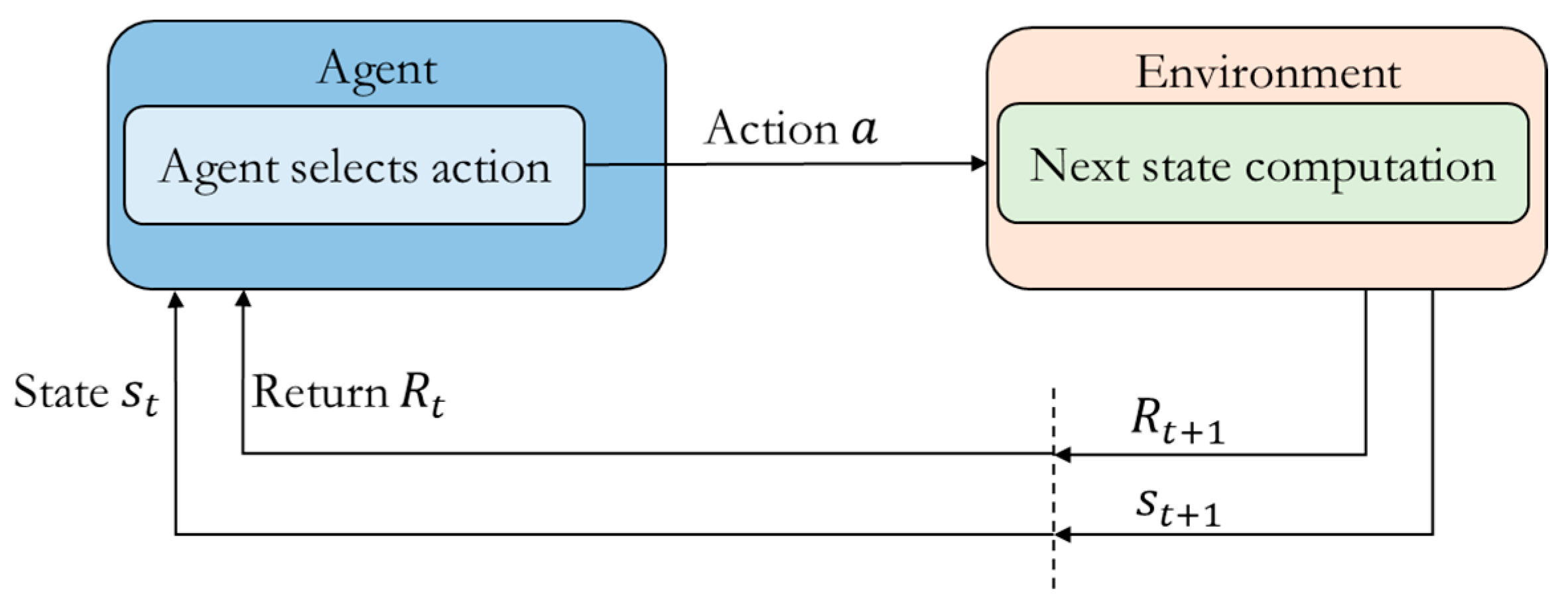
Reinforcement learning (RL) algorithms consist of five main components: the agent, the environment, the state, the action A, and the observation R. At time step t, the agent generates action $a$ and interacts with the environment. After executing the action, the agent’s state transitions from $s_t$ to $s_{t+1}$, and the agent receives an environment return value $R_{t+1}$. Through this process, the agent dynamically modifies its data during interactions with the environment. After a sufficient number of interactions, the agent acquires an optimized action policy. The agent-environment interaction process is illustrated in Figure 4 below.

The computational process of RL is an ongoing exploration to optimize strategies. The aforementioned strategy refers to the mapping from states to actions. The following formula provides the probability of selecting action $a$ for state $s$:

$$\pi \left(a\right|s)=p[A_t=a|S_t=s]$$

(13)

By employing RL algorithms, our objective is to maximize the action value of the corresponding state:

$${\pi }^{*}\left(a|s\right)=\underset{a\in A}{\mathit{argmax}}{Q}^{*}\left(a|s\right)$$

(14)

Traditional RL methods store state and action value function values in tabular form. While this approach enables rapid acquisition of required state and action values for simple problems, it struggles with complex scenarios. Deep learning integrates feature learning into the model, endowing it with self-learning capabilities and robustness to environmental changes, making it suitable for nonlinear models. However, deep learning cannot achieve unbiased estimation of data rules. Moreover, this approach requires large labeled datasets and repeated computations to achieve high prediction accuracy. Based on the above analysis, when tackling complex nonlinear problems, it is feasible to construct DRL algorithms by combining deep learning with RL algorithms and applying them to solve complex issues.

PPO stands as one of the most widely employed DRL algorithms today. Building upon the trust region policy optimization (TRPO) algorithm, it optimizes the following objective function:

$${\mathcal{L}}^{CLIP}\left(\theta \right)={\mathbb{E}}_t\left[min\left\{r_t\left(\theta \right)A_t, clip\left(r_t\right(\theta ),1-\epsilon ,1+\epsilon )A_t\right\}\right]$$

(15)

Among these, $r_t\left(\theta \right)$ represents the probability ratio between the old and new strategies introduced by importance sampling, calculated as follows:

$$r_t(\theta )={\displaystyle \frac{{\pi }_{\theta }\left(a_t\right|s_t)}{{\pi }_{old}\left(a_t\right|s_t)}}$$

(16)

$A_{\pi }(s,a)$ represents the dominance function, indicating how much the value of choosing action $a$ is higher than the average value under the current state $s$. Its calculation method is as follows:

$$A_{\pi }\left(s,a\right)=Q_{\pi }\left(s,a\right)-V_{\pi }\left(s\right)$$

(17)

Since the true value of the advantage function is unknown, an appropriate method must be employed to estimate it. References [28,29] utilize the state value function $V\left(s_t\right)$ and apply generalized advantage estimation (GAE) techniques to estimate the advantage function. Reference [30] employs finite-horizon estimators (FHE) for advantage function estimation. Considering the characteristics of sample sequences and network update mechanisms, this paper utilizes GAE to pre-estimate the action advantage function, with the calculation method outlined below:

$${\widehat{A}}_t={\sum }_{l=0}^{\infty }{\left(\gamma \lambda \right)}^l{\delta }_{t+l}^V$$

(18)

When $\gamma =1$, the calculation methods for the estimated advantage function in GAE and FHE are equivalent. ${\delta }_{t+l}^V$ represents the one-step temporal differential error, calculated as follows:

$${\delta }_{t+l}^V=r_t+\gamma V\left(s_{t+1}\right)-V\left(s_t\right)$$

(19)

Incorporating policy entropy into the optimization function of the PPO algorithm [30,31,32] enhances the agent’s exploration capability for unknown policies. Policy entropy is defined as follows:

$$\mathcal{H}\left(\pi \right)={\mathbb{E}}_{\pi }\left[-log\pi \left(a\right|s)\right]$$

(20)

The optimization function for increasing strategy entropy is as follows:

$$J_{\theta }={\mathcal{L}}_{\theta }^{CLIP}+{\beta }_E\mathcal{H}\left({\pi }_{\theta }\right)$$

(21)

where ${\beta }_E$ is the temperature coefficient.

Reference [33] proposes an improved PPO algorithm that constructs an objective function integrating policy network optimization, value network optimization, and policy entropy. It employs a parameter-sharing mechanism between the policy and value networks to enhance algorithmic efficiency. Experimental results demonstrate that the proposed algorithm inherits the advantages of TRPO while offering simpler implementation and greater generalization capability. Drawing upon the network parameter sharing mechanism and objective function construction methods from the aforementioned literature, this paper establishes the following objective function based on the constructed policy network optimization function:

$$J_{\theta }^{AC}={\mathcal{L}}_{\theta }^{CLIP}+{\beta }_E\mathcal{H}\left({\pi }_{\theta }\right)+{\mathcal{L}}_{\theta }^{VF}$$

(22)

Among these, ${\mathcal{L}}_{\theta }^{VF}$ denotes the squared-error loss, representing the optimization objective function for the value network. Its calculation method is as follows:

$${\mathcal{L}}_{\theta }^{VF}={\mathbb{E}}_t\left[{(r_t+\gamma V\left(s_{t+1}\right)-V\left(s_t\right))}^2\right]$$

(23)

Assuming PPO uses a trajectory sequence with a fixed time step T to update its network structure, the algorithm’s workflow is as follows. First, in each episode, each actor network receives data over a time step T with a network size of N. Next, based on this data, the agent loss function $J_{\theta }^{AC}$ is constructed and optimized using the Adam optimizer [34] for k epochs. Then, in the subsequent episode, the updated network parameters are used to generate an action policy, and the iterative cycle continues. The pseudocode for PPO is shown in Algorithm 1.

Algorithm 1 PPO, actor-critic style
1	for episode = 1,2,$\cdots$do
2	for actor = 1,2,$\cdots$N do
3	Implementation strategy ${\pi }_{old}$, cumulative time step T;
4	Using GAE technology to calculate advantage estimates ${\widehat{A}}_1, {\widehat{A}}_2, \cdots$, ${\widehat{A}}_T$;
5	end for
6	Optimize the loss function $J_{\theta }^{AC}$ using the Adam optimizer to obtain new network parameters;
7	Update the parameters of the policy network and value network ${\theta }_{old}\leftarrow \theta$;
8	end for

3.1.2. ARMH-PPO Algorithm

Building upon the fundamental architecture of the PPO algorithm and considering the characteristics of UAV evasion maneuvers against missiles as well as the requirements of actual missions, targeted improvements are made to the PPO algorithm. These modifications encompass the action space, state space, reward function, and network architecture.

(1)

Hierarchical maneuver action space

The action space of classical DRL algorithms encompasses types such as discrete action space, continuous action space, multidimensional discrete action space, and hybrid action space. Drawing on action space modeling methods for air-to-air mission agents, we model the action space for UAV missile evasion. Common approaches to air-to-air mission action space modeling include the following:

The action space in the air-to-air mission exhibits continuous characteristics. Some studies utilize aircraft control stick and throttle stick deflections as maneuver control variables, solving for these variables via intelligent algorithms. In the AlphaDogFight competition, Lockheed Martin employed aircraft stick and throttle deflection as agent action parameters, solving these parameters using a DRL algorithm that outputs deflections for elevator, rudder, aileron, and throttle [35]. References [36,37] selected tangential overload, normal overload, and roll angle as the agent’s action control variables. Since this paper employs a 6-DOF UAV dynamics model, the action space modeling method from [35] can be adapted, and the proposed algorithm can be used to solve for the UAV’s maneuver control variables. However, the aforementioned action space modeling method has the following shortcomings: Since existing flight control knowledge is not integrated into the algorithm, it must learn both maneuver strategies and flight control; that is, the decision-making performance of the algorithm is tightly coupled with the UAV platform. This hinders stable aircraft control and makes the agent training process difficult to converge.

To enhance agent training efficiency, some studies have discretized the action space for air-to-air mission and modeled it as a discrete action space. This approach first constructs a maneuver action set, from which the agent selects the optimal maneuver action during each decision-making instance. Reference [38] proposes a matrix game algorithm to address autonomous maneuver decision-making in air-to-air mission. The discrete action space constructed in this work comprises seven fundamental maneuvers: constant velocity, maximum acceleration climb, maximum acceleration descent, maximum G-load left turn, maximum G-load right turn, maximum G-load climb, and maximum G-load dive. These basic maneuvers are simple to implement, and the agent can achieve complex maneuvers by selecting different combinations of actions. However, these basic actions primarily consider the extreme cases of aircraft flying at maximum acceleration and maximum g-load, which do not align with the actual air-to-air mission process.

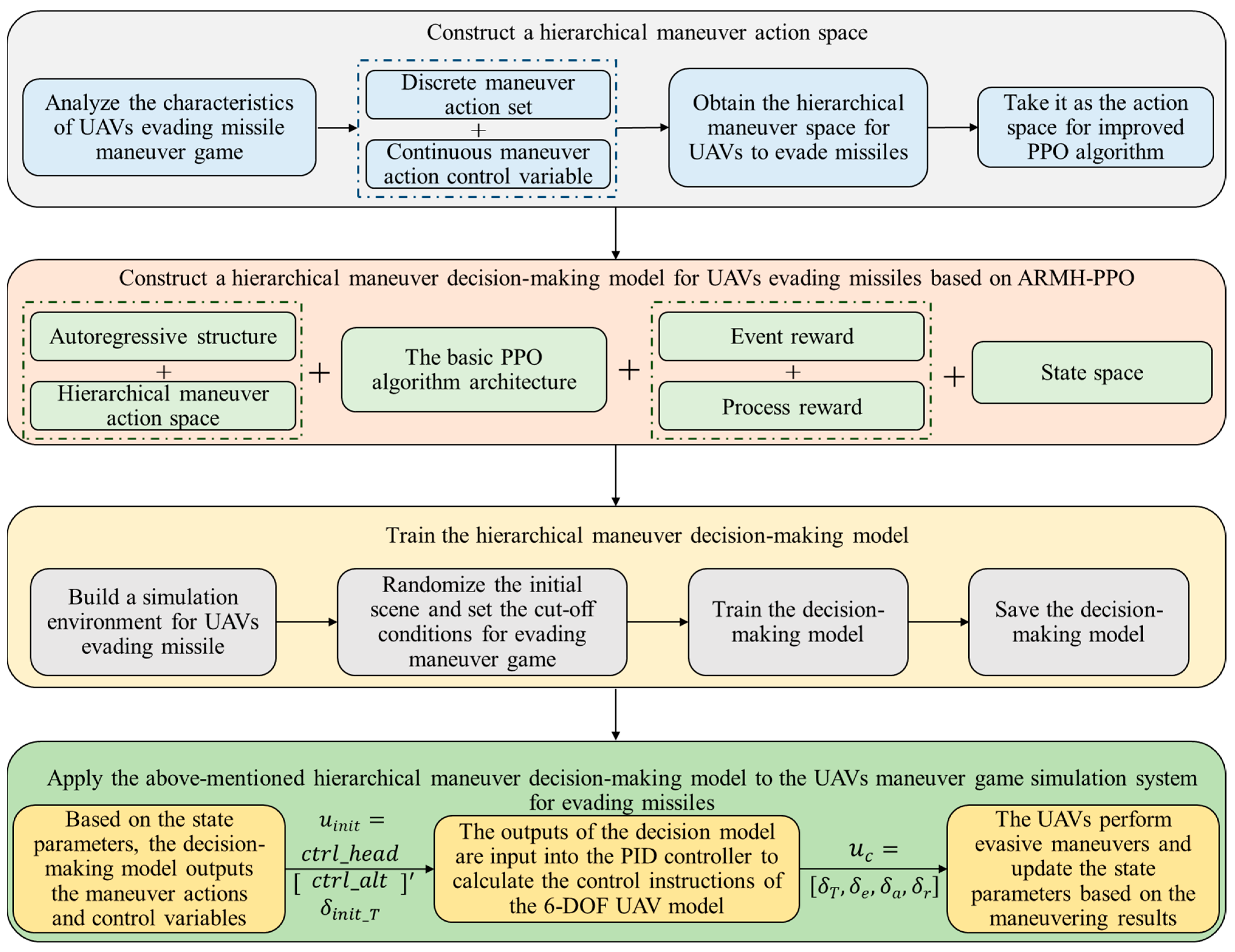
Based on the aforementioned research and considering the practical requirements of UAV evasion maneuvers against missiles as well as the need for multi-platform transferability of decision models, this paper constructs a hierarchical maneuver action space as shown in

Table 3. Hierarchical maneuver action space.

Number	Action	Control Variables
0	pull up	heading, altitude, throttle stick deflection
1	circling	heading, altitude, throttle stick deflection
2	steep turn	heading, altitude, throttle stick deflection
3	loop	heading, altitude, throttle stick deflection
4	level flight	heading, altitude, throttle stick deflection
5	s-maneuver	heading, altitude, throttle stick deflection
6	climb	heading, altitude, throttle stick deflection
7	dive	heading, altitude, throttle stick deflection

. Since this maneuver space incorporates both discrete action sets and continuous maneuver control variables, it constitutes a hybrid action space. As shown in Table 3, the discrete action set comprises eight maneuvers [39]: pull-up, turn, sharp turn, barrel roll, level flight, S-maneuver, climb, and dive. The pull-up maneuver is introduced to prevent the UAV from breaching minimum altitude restrictions, while the dive maneuver is employed to lure the missile into lower altitude layers. This strategy leverages the increased aerodynamic drag at lower altitudes to dissipate the missile’s kinetic energy, thereby mitigating the threat posed by the missile. Based on the above eight fundamental maneuvers, the agent selects appropriate combinations of different actions to drive the UAV to execute complex evasive maneuvers.

The control variables in the action space are heading, altitude, and throttle stick deflection. During training episodes, at each decision point, the UAV evasion missile hierarchical maneuver decision model selects optimized control variables from the continuous maneuver control variables based on current state features and the chosen maneuver type. The continuous maneuver control variable ranges are shown in

Table 4. Control variable value range.

Control Variable Type	Value Range
heading	[−1, 1]
altitude	[−1, 1]
throttle stick deflection	[0, 1]

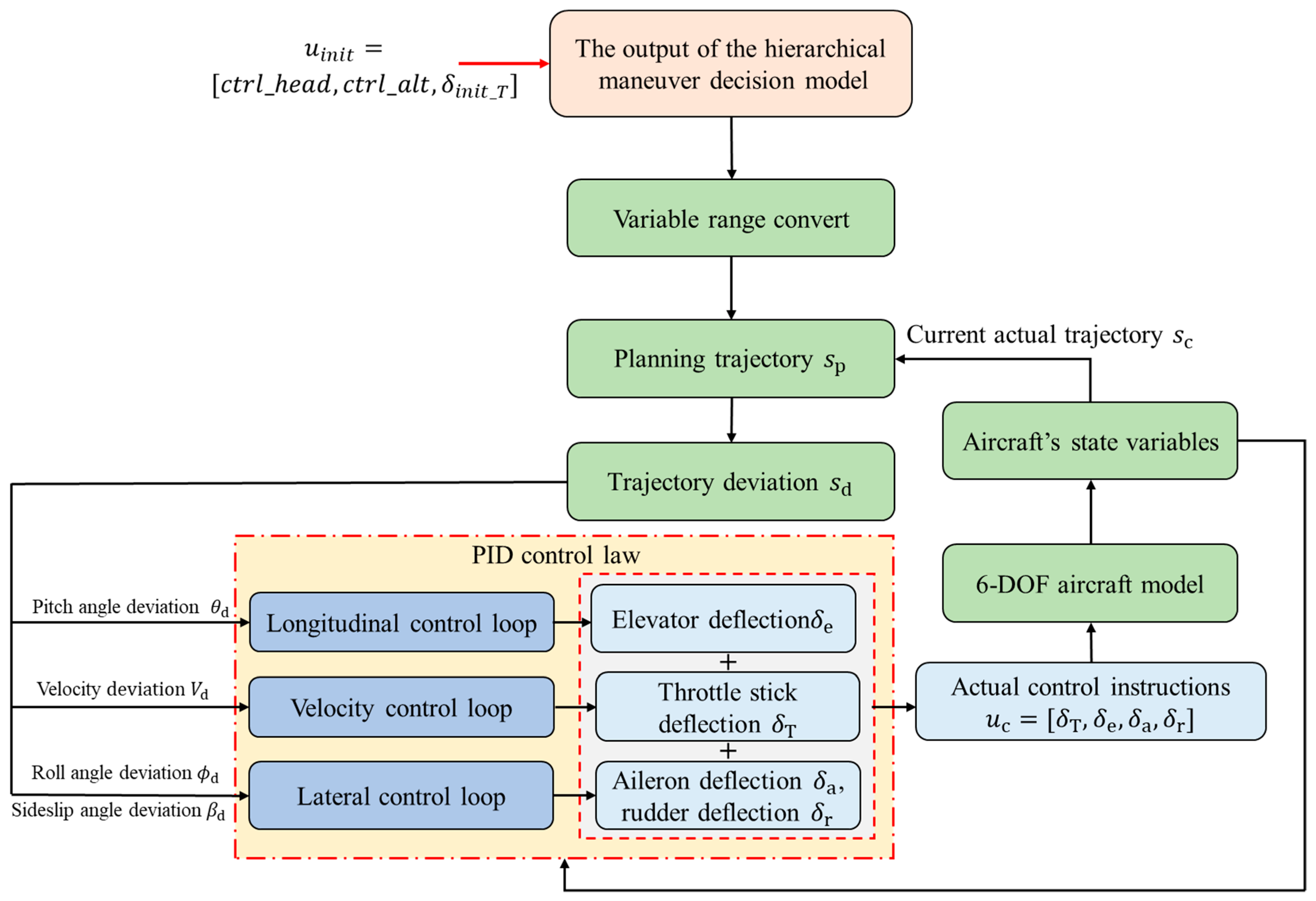
. The control variable ranges in Table 4 are normalized. First, the agent solves for heading, altitude, and throttle stick control variables via the evasion maneuver decision algorithm. Next, a transformation function converts these into planned heading, altitude, and throttle stick deflection values. Then, a PID controller [27] solves for elevator, rudder, aileron, and throttle stick deflections. Finally, the resulting stick and throttle deflections are input to the 6-DOF UAV motion model to drive the execution of evasive maneuvers.

This paper constructs a hierarchical maneuver space to decouple the decision algorithm from the simultaneous learning of flight control and evasive maneuver strategies. This approach not only reduces the complexity of evasive maneuver decision-making but also addresses the issue of limited model transferability across platforms. Furthermore, by normalizing the range of maneuver control inputs, the approach prevents extreme scenarios where the aircraft frequently operates at maximum acceleration and overload due to control values exceeding preset limits. This ensures the UAV’s maneuvering actions align with real-world capabilities.

(2)

State space

During UAV missile evasion, the state space in DRL is constructed by extracting partial UAV state variables and the relative motion characteristics between the missile and UAV. To capture the dynamic evolution of the evasion maneuvering game between the UAV and missile, the following 10 state variables are employed to construct the algorithm’s state space [40]: relative distance between UAV and missile $R_{um}$, missile elapsed time $t_m$, relative heading angle ${\psi }_u-{\psi }_m$, UAV’s velocity $V_u$, UAV’s altitude $z_u$, UAV’s yaw angle ${\psi }_u$, missile’s velocity $V_m$, missile’s altitude $z_m$, missile-to-UAV LOS inclination angle change rate ${\dot{\epsilon }}_r$, and LOS declination angle change rate ${\dot{\beta }}_r$.

To eliminate the adverse effects of differing ranges for these 10 state variables on algorithm training performance, each state variable must undergo normalization processing before inputting them into the evasion missile hierarchical maneuver decision model for training. This ensures consistent input parameter ranges for the model. The expressions for normalizing each state variable are as follows.

$$S_i^{normal}=\left(2\cdot {\displaystyle \frac{S_i-S_i^{min}}{S_i^{max}-S_i^{min}}}\right)-1, iϵ\{\mathrm{1,2},3,\cdots ,10\}$$

(24)

Here, $i$ represents the status variable type identifier, which follows the same sequence as the order of status variables in the state space; $S_i$ denotes the status variable type currently undergoing normalization processing; $S_i^{min}$ and $S_i^{max}$, respectively, indicate the minimum and maximum values of the current status variable; and $S_i^{normal}$ is the normalized value of the current status variable.

(3)

Reward function

The reward function plays a crucial role in DRL algorithms. The inherent reward function for the UAV missile evasion problem provides a reward at the end of each round based on the outcome of that round. However, such rewards are overly sparse, making it difficult to guide the agent toward learning an optimal strategy. To address the issue of reward sparsity, ref. [41] employs reward-shaping techniques. This approach introduces process rewards to guide the agent’s training process. Based on [39,42], a reward function for the UAV missile evasion problem is designed as shown in

Table 5. Reward function for UAV missile evasion.

Type	Name	Value
Event Rewards	UAV crashes to ground	−1
	UAV hit by missile	−1
	UAV’s speed below set minimum	−1
	Missile crashes to ground	+1
	Missile’s speed below set minimum	+1
	UAV performs close-range evasion maneuver	+1
	Exceeded maximum simulation time	+1
	Missile loses target	+1
Process Rewards	Relative distance between missile and UAV	$R_{redist}$
	UAV’s altitude	$R_{reheight}$
	LOS declination angle between missile and UAV	$R_{losdeclin}$
	LOS inclination angle between missile and UAV	$R_{losinclin}$

.

This paper categorizes rewards into event-based and process-based rewards. Event-based rewards are sparse, granted only upon the occurrence of specific events. Process-based rewards are dense and calculated at every time step. This category includes UAV altitude, missile-to-UAV relative distance, missile-to-UAV LOS declination angle, and LOS inclination angle. The UAV altitude reward reflects the aircraft’s potential energy advantage. This reward incentivizes the agent to execute climb maneuvers, thereby accumulating higher terminal energy. This approach enables the UAV to prioritize its own safety while leveraging its energy advantage, providing essential support for subsequent air-to-air missions. The calculation method for the UAV altitude reward is as follows.

$$R_{reheight}=c_1{\displaystyle \frac{z_u\left(t\right)}{z_u\left(t_0\right)}}$$

(25)

$z_u\left(t\right)$ and $z_u\left(t_0\right)$ denote the UAV’s altitude at time t and its initial altitude, respectively; $c_1$ is a positive coefficient primarily used to adjust the range of values for the altitude reward function.

The relative distance between the missile and the UAV refers to the distance between the UAV and the missile, which is updated at each time step. When the relative distance is less than or equal to the missile’s kill radius $r_d$, the UAV is hit by the missile, and the agent receives a penalty. When the relative distance exceeds the missile’s kill radius $r_d$, the agent receives a reward proportional to the magnitude of the distance between the UAV and the missile. This incentivizes the agent to execute tailing maneuvers or tangential maneuvers, thereby increasing the relative distance or slowing the rate of approach, thus enhancing the UAV’s survivability. The calculation method for the missile-UAV relative distance reward is as follows.

$$R_{redist}=\left\{\begin{array}{l}{c}_2‖r\left(t\right)‖/‖r\left(t_0\right)‖ ‖r\left(t\right)‖>r_d\\ -1 ‖r\left(t\right)‖\le r_d\end{array}\right.$$

(26)

$‖r\left(t\right)‖$ and $‖r\left(t_0\right)‖$ denote the relative distance and initial relative distance between the UAV and missile at time t, respectively; $c_2$ is a positive coefficient primarily used to adjust the value range of the relative distance reward function.

The LOS declination angle between the missile and the UAV refers to the angle between the horizontal projection of the LOS vector and the horizontal coordinate axis. As the LOS declination angle increases, the missile is forced to turn to maintain tracking of the UAV, consuming missile energy and increasing the UAV’s success rate in evading the missile. Under the aforementioned conditions of increased LOS declination angle, the reward value obtained by the agent for this parameter increases, which helps guide the agent to execute turning maneuvers. The calculation method for the LOS declination angle reward between the missile and UAV is as follows [43].

$$R_{losdeclin}=c_3{e}^{{\displaystyle \frac{{\beta }_r^2\left(t\right)}{k_1}}}/e^{{\displaystyle \frac{{\beta }_r^2\left(t_0\right)}{k_1}}}$$

(27)

${\beta }_r\left(t\right)$ and ${\beta }_r\left(t_0\right)$ denote the LOS declination angle between the UAV and missile at time t and initial LOS declination angle, respectively; $k_1$ and $c_3$ are positive coefficients primarily used to adjust the value range of the LOS declination angle reward function.

The LOS inclination angle between a missile and a UAV refers to the angle between the LOS vector and the horizontal plane. An increased LOS inclination angle induces the missile to follow the maneuver, thereby consuming missile energy and disrupting its stable tracking conditions. When the LOS inclination angle is negative and its absolute value increases, the agent receives a higher reward value for this parameter. This encourages the agent to execute a dive maneuver, which accelerates missile energy depletion by leveraging greater air resistance at low altitudes while simultaneously disrupting the seeker’s tracking conditions using ground clutter at low altitudes. The calculation method for the LOS inclination angle reward between the missile and UAV is as follows [43].

$$R_{losinclin}{=c}_4{e}^{-{\displaystyle \frac{{\epsilon }_r\left(t\right)}{k_2}}}/e^{-{\displaystyle \frac{{\epsilon }_r\left(t_0\right)}{k_2}}}$$

(28)

${\epsilon }_r\left(t\right)$ and ${\epsilon }_r\left(t_0\right)$ denote the LOS inclination angle between the UAV and missile at time t and initial LOS inclination angle, respectively; $k_2$ and $c_4$ are positive coefficients primarily used to adjust the value range of the LOS inclination angle reward function.

It should be noted that in the reward functions described above, the coefficients $k_1$, $k_2$ and $c_1~c_4$ serve to eliminate the impact of differences in the value ranges of individual reward functions on the overall reward function. Literature [39,43] provides detailed introductions and experimental analyses regarding the setting of these coefficients. This paper adopts the relevant coefficient setting methods from the aforementioned references.

By integrating the event reward values from Table 5 and the process reward function calculations described above, we compute the overall event reward and overall process reward separately. Building upon this foundation, we draw inspiration from exploratory learning theory to design a temporal decay factor. This factor is multiplied by the overall process reward, and the resulting reward is then added to the overall event reward to yield the algorithm’s total reward. The calculation method for the overall event reward $R_{allevent}$ is as follows.

$$R_{allevent}={\sum }_{i=1}^8{R}_i$$

(29)

$R_i$ denotes the reward received by the agent after the event that terminates the current training episode occurs. $R_1$ to $R_8$ represent the following rewards, respectively: UAV landing reward, UAV hit by missile reward, UAV speed less than the set minimum speed reward, missile landing reward, missile speed less than the set minimum speed reward, UAV close-range evasion of missile reward, exceeding the maximum simulation time reward, and missile loss of target reward. During each training episode, not all eight events listed above necessarily occur. Only when the triggering condition for a specific event is met will its reward be assigned; rewards for other events are set to zero during that episode.

The calculation method for the overall process reward $R_{allprocess}$ is as follows.

$$R_{allprocess}=R_{redist}+R_{reheight}+R_{losdeclin}+R_{losinclin}$$

(30)

At each time step, the process rewards described above are first assigned different values based on the relative posture between the UAV and the missile. The total process reward for that time step is then obtained by summing all process rewards.

The calculation method for the overall algorithm reward $R_{algall}$ is as follows.

$$R_{algall}=k_{eve}{\cdot R}_{allevent}+k_{pro}{\cdot e}^{-k_{3}n}{R}_{allprocess}$$

(31)

$e^{-k_{3}n}$ serves as a temporal decay factor, designed to minimize undue human influence on the agent during strategy exploration. n represents the current training episode count of the UAV evasion maneuver decision-making model. $k_{eve}$ and $k_{pro}$ represent the weight coefficients for event rewards and process rewards, respectively, with $k_{eve}$+$k_{pro}=1$. They are primarily used to adjust the influence of these two reward types on the agent’s training process. $k_3$ is the attenuation coefficient of process rewards, which is mainly used to control the attenuation rate of the influence of process rewards on the agent’s policy search process. Since event rewards are sparse, relying solely on them to guide model training would hinder convergence and prevent the agent from learning effective strategies. The introduction of process rewards integrates expert knowledge into the training process, guiding the agent to search for optimized strategies during the early stages of algorithm iteration. In the later stages of model training, the agent has developed a certain capacity for strategy optimization. At this point, the role of process rewards diminishes, meaning the influence of expert experience on the model training process decreases. The agent primarily relies on event rewards to guide its autonomous exploration of strategies.

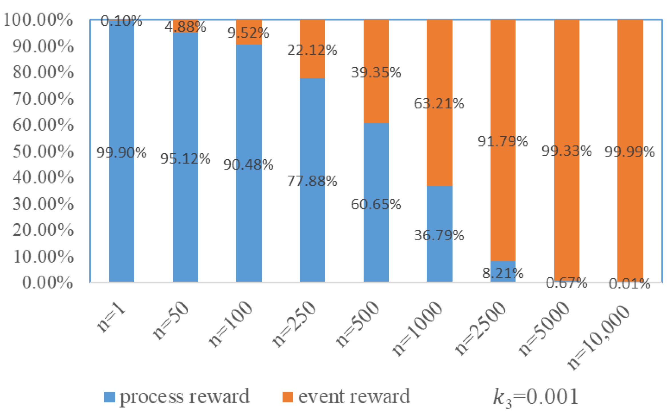
When $k_3$= 0.001, as n increases, the proportion of event rewards and process rewards in the overall algorithmic reward varies with the count of training episodes, as shown in Figure 5. During the initial phase of training the evasive maneuver decision-making model, event rewards account for a smaller proportion. At this stage, expert experience primarily guides the agent in searching for maneuver strategies. As training progresses, when the model reaches 1000 training episodes, event rewards constitute 63.21% of the total. At this point, the role of expert experience in guiding the agent’s search for maneuver strategies diminishes, and the agent increasingly relies on autonomous exploration to search for maneuver strategies. By the 2500th episode, event rewards reach 91.79%. At this point, the guiding influence of process rewards on the agent’s maneuver strategy search further diminishes. This helps mitigate the limitation where the agent’s learning process is overly influenced by expert knowledge, which would otherwise confine its autonomous maneuver decision-making capabilities to the level of expert knowledge. Furthermore, the guiding role of process rewards during the early training phase prevents the agent from engaging in excessive blind exploration, which is beneficial for accelerating the convergence of the UAV evasive maneuver decision-making model training process.

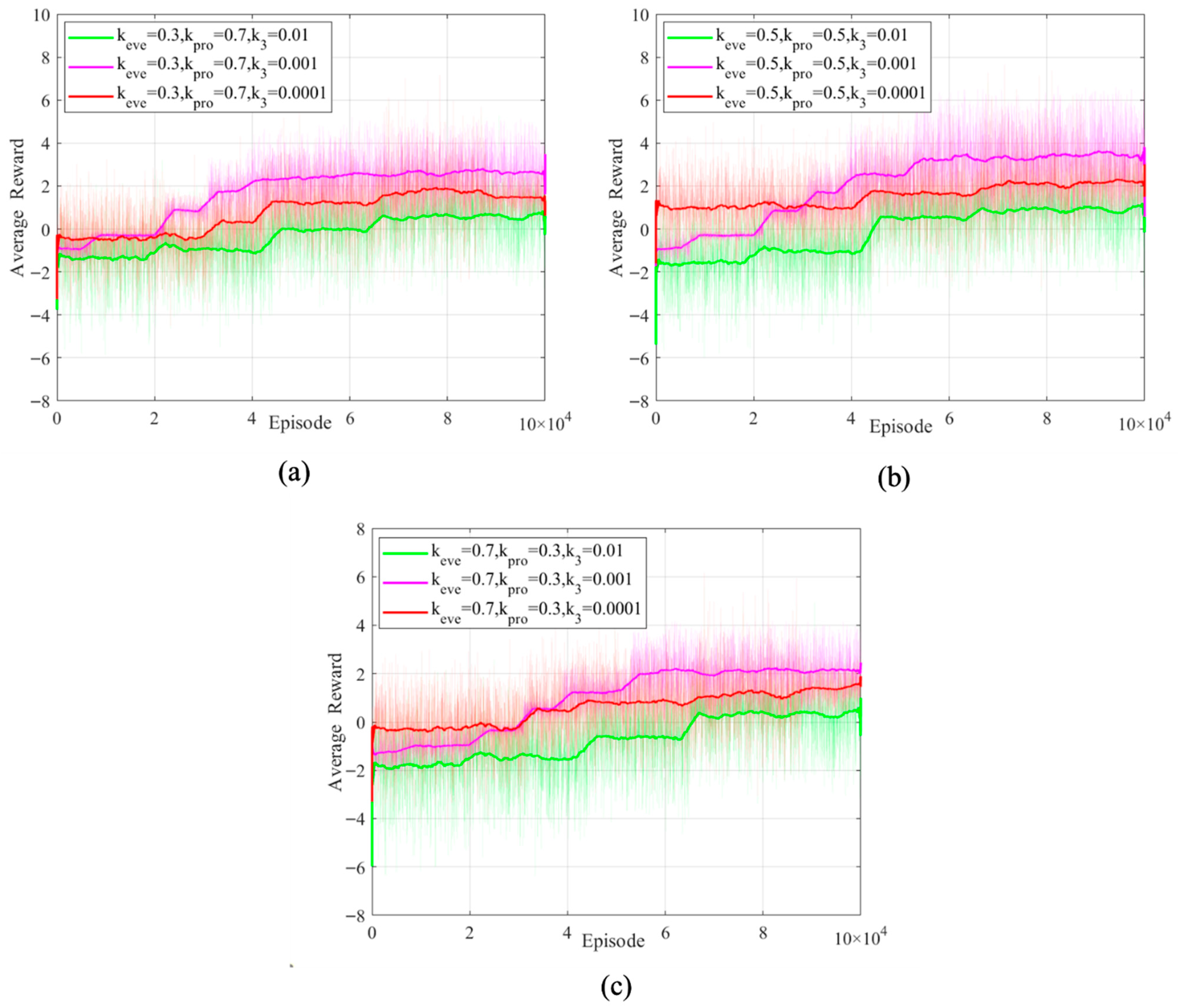
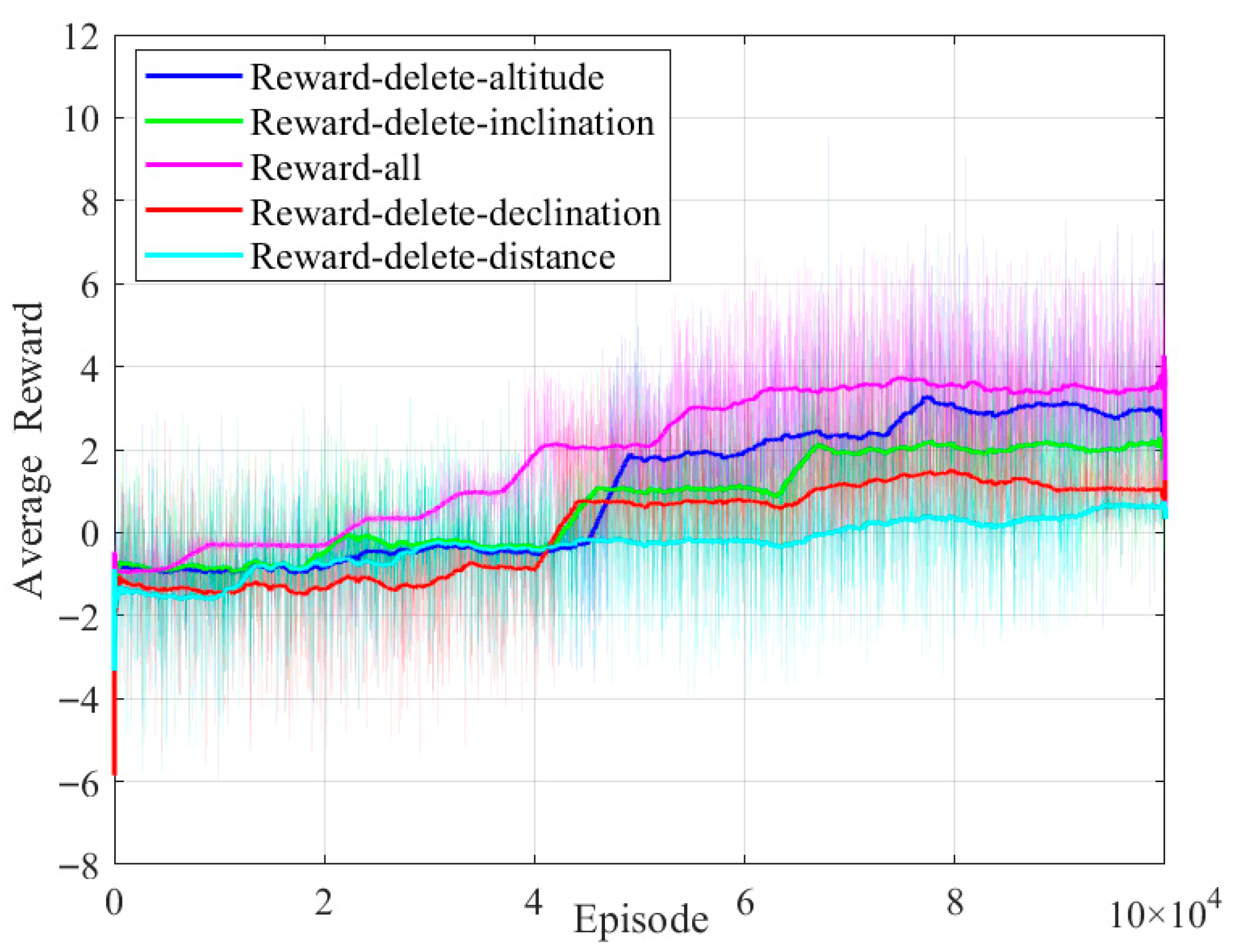
Next, comparative experiments are conducted on the values of $k_{eve}$, $k_{pro}$, and $k_3$ to determine their optimal settings. During the training of the UAV evasion maneuver decision-making model, statistical analysis of the average reward value’s variation with training episodes provides support for determining these parameters. Figure 6 illustrates the curve depicting the average reward value’s change.

Under different combinations of reward weight coefficients, when $k_{eve}=0.5$ and $k_{pro}=0.5$, the average maximum reward value in Figure 6b exceeds that of the other two combinations. With fixed reward weight coefficients, when $k_3=0.01$, the agent achieves the lowest average reward value. When $k_3=0.001$, the agent ranks second in average reward during the early training phase and first in the late training phase. When $k_3=0.0001$, the agent achieves the highest average reward during the early training phase, but the average reward growth slows significantly in the later training phase. This is primarily attributed to the parameter setting favoring expert knowledge guidance during the initial training process. However, this also tends to confine the agent’s evasive maneuver decision-making to expert-level capabilities, limiting its ability to explore new strategies. Based on the above analysis, this paper sets the reward weighting coefficient and process reward decay coefficient as follows: $k_{eve}=0.5,k_{pro}=0.5$, $k_3=0.001$.

(4)

Network architecture

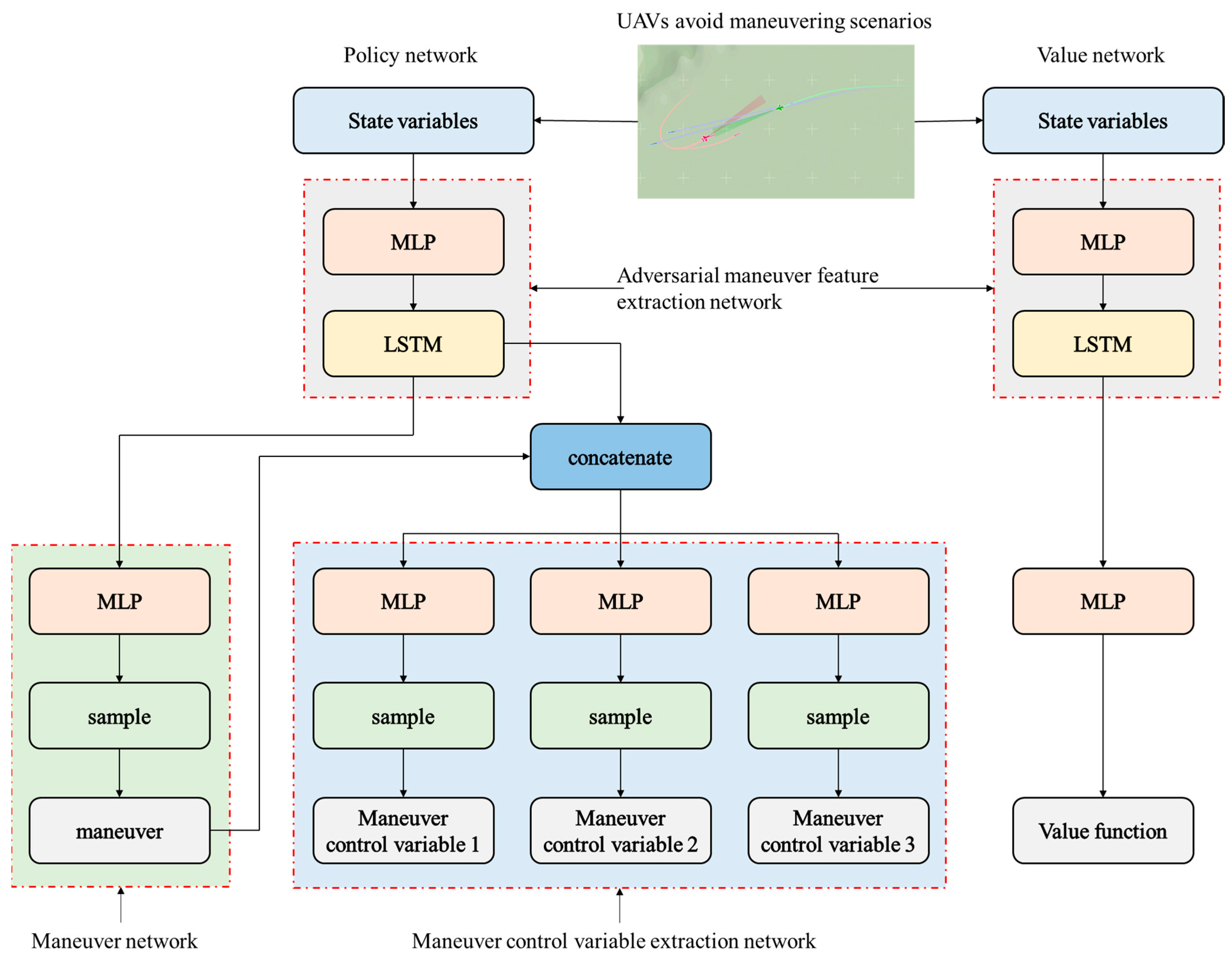
By adopting the PPO algorithm framework from Section 3.1.1 and the state space, action space, and reward function design methods proposed in this section, this paper presents an improved PPO algorithm, namely the ARMH-PPO algorithm. Its main structure is illustrated in Figure 7. The ARMH-PPO algorithm retains most settings of the PPO algorithm and adopts an actor-critic structure comprising a policy network and a value network. The policy network outputs evasive maneuvers based on the current state, while the value network evaluates the current state and outputs an estimate of the state value function. 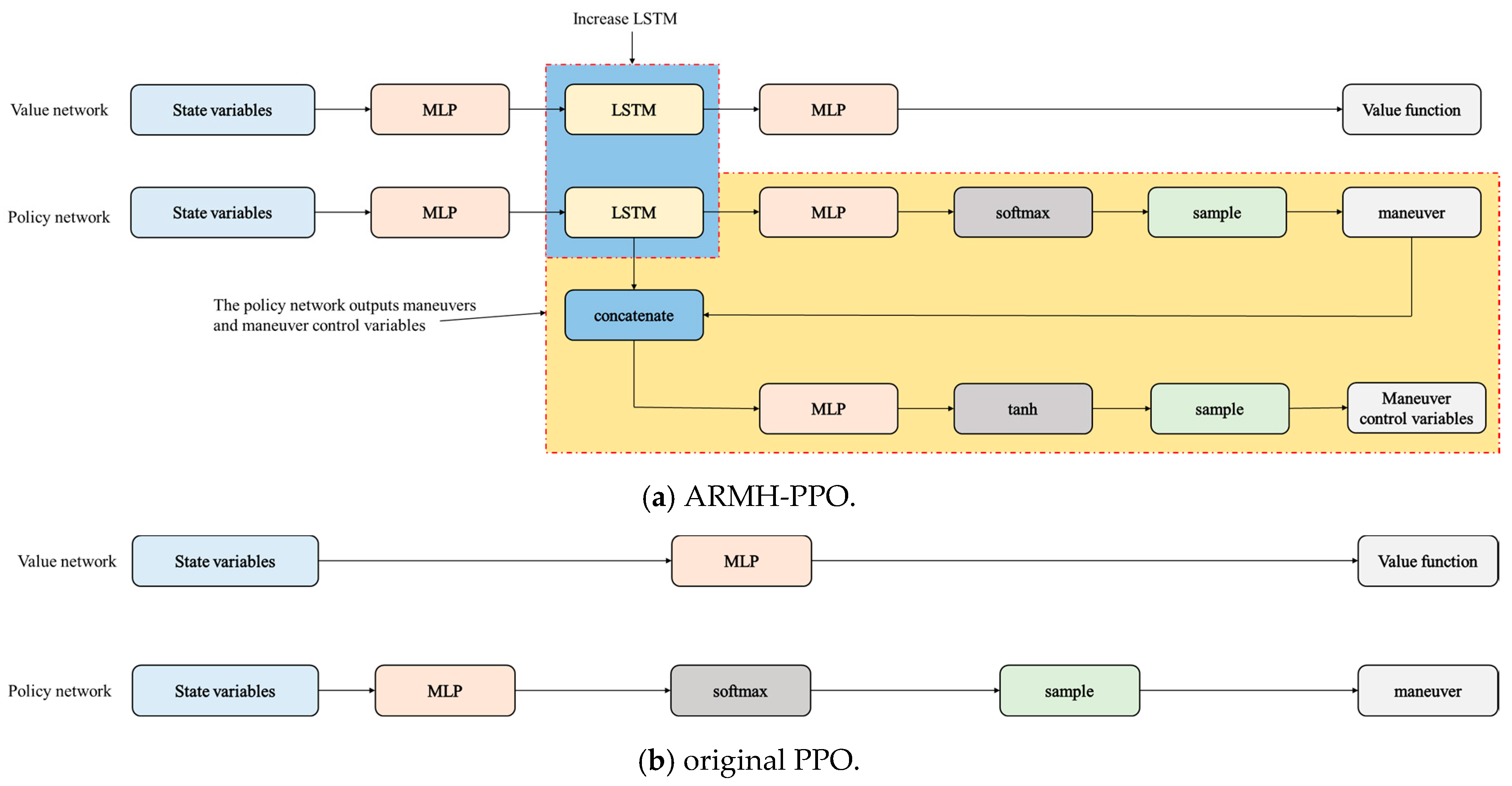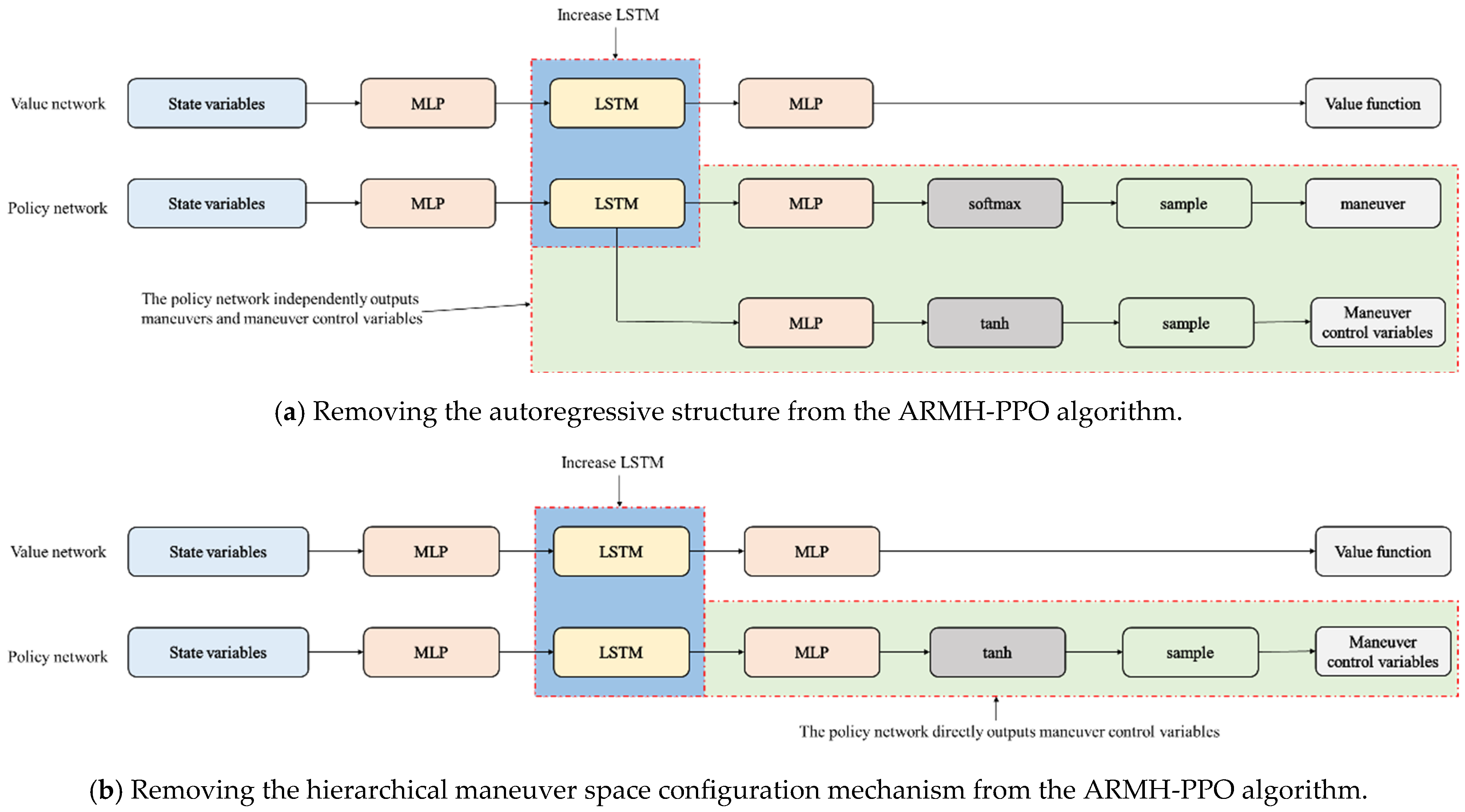Figure 8 compares the original PPO algorithm architecture with the ARMH-PPO algorithm structure. Compared to the original PPO algorithm, the ARMH-PPO algorithm introduces the following key improvements:

(1) Incorporate LSTM networks into the policy network and value network. Given that UAV evasion maneuver decision-making exhibits sequential decision characteristics, and considering LSTM’s superiority over fully connected networks in processing time series data [44], LSTM is employed to process observations during the evasion maneuver game process, thereby extracting features from the game time series. The adversarial feature extraction network depicted in Figure 7 illustrates this methodology.

(2) By adopting an autoregressive structure, the improved PPO algorithm is made applicable for solving problems involving both discrete actions and continuous control variables within hierarchical maneuver action spaces. The traditional PPO algorithm is only applicable to decision-making in a single action space, i.e., scenarios involving either continuous actions or discrete actions. Decision models constructed based on this method struggle to address evasive maneuver decision problems across different UAV and missile platforms. To address the hierarchical maneuver action space proposed in this paper and uncover the relationship between maneuver action types and maneuver action control variables—thereby enhancing the stability of UAV evasive maneuvers—the policy network is modified. The improved policy network comprises a maneuver action network and a maneuver action control variable network, as illustrated in Figure 7. The maneuver action network outputs selection probabilities for each action within the discrete action set, with maneuvers obtained through sampling; The maneuver control variable network adopts an autoregressive-like structure. It takes the UAV evasion maneuver adversarial features extracted by LSTM and the sampled maneuvers as inputs. First, subnetworks separately output the mean of the continuous action control variables. Then, combining the variance of the maneuver control variables, a normal distribution is constructed. Finally, the maneuver control variables are sampled from this distribution. In the ARMH-PPO algorithm, a complete action a comprises the maneuver type m and the corresponding maneuver control variable x. Since different maneuvers have distinct control variable ranges, a strong correlation exists between maneuver control variables and types. To reinforce this relationship, an autoregressive form is adopted, explicitly requiring maneuver types as inputs to the maneuver control variable network. Thus, the relationship between maneuver types and control variables is defined as follows:

$$x=f(z,m)$$

(32)

Here, z represents the evasive maneuver countermeasure features extracted by the LSTM network, m denotes the sampled maneuver type, x is the corresponding control variable for the maneuver, and $f(·)$ is the function represented by the maneuver control variable network. Since the maneuver type m is also the output of the policy network—meaning the policy network uses its own output as input—this resembles the autoregressive text generation approach in Chinese information processing. Therefore, borrowing the concept of autoregression, the algorithm is said to possess the characteristic of autoregressive generation of maneuvers. In Section 4.2.2, the effectiveness of the autoregressive structure is validated through the implementation of ablation experiments.

3.2. Hierarchical Maneuver Decision-Making Process and Parameter Selection for UAV Missile Evasion Based on ARMH-PPO

Using the ARMH-PPO algorithm designed in Section 3.1, a hierarchical maneuver decision model for UAV evasion against incoming missiles is constructed. This section primarily introduces the training process for the aforementioned decision model, hierarchical maneuver decision flow, and algorithm hyperparameter selection.

3.2.1. Training of Decision Model Based on ARMH-PPO

During the training process of the decision-making model, for a given random initial scenario, the UAV continuously outputs maneuver action types and control variables based on its existing decision network. It then iteratively updates state parameters, reward values, and the termination flag for the current episode based on these outputs. The episode termination flag is determined by the termination conditions of the UAV’s evasive maneuvering against missiles. Its primary function is to conclude the current episode, save the relevant information generated during this episode, and then re-randomize the initial scenario to initiate a new simulation round. This process generates training data across multiple scenarios. The following sections primarily introduce the termination conditions for the UAV’s evasive maneuvering against missiles and the decision model training workflow.

(1)

UAV missile evasion maneuver countermeasure process termination criteria

(1)

Missile evasion failure

If at a certain moment t during the UAV’s missile evasion process, the following conditions are met, it is considered that the UAV has been hit by the missile and the evasion has failed:

$$‖r\left(t\right)‖\le r_d, V_m\left(t\right)\ge V_{m min}, t\le t_w$$

(33)

$V_{m min}$ is the minimum controllable velocity of the missile; $t_w$ is the operational duration of the missile engine; $r_d$ is the kill radius of the missile.

If the UAV’s altitude exceeds the preset altitude range at any given moment, it is deemed to have touched down, resulting in evasion failure:

$$z_u\left(t\right)\le z_{u min}, t\le t_{max\_time}$$

(34)

$z_{u min}$ is the minimum flight altitude of the UAV; $t_{max\_time}$ is the maximum simulation time.

• (2)

  Missile evasion successful

If at any point $t$ during the UAV’s evasion maneuver the following conditions are met, the UAV’s evasion is considered successful:

$$z_m\left(t\right)<z_{m min}, t\le t_{max\_time}$$

(35)

$$V_m\left(t\right)<V_{m min}, t\le t_{max\_time}$$

(36)

$$‖r\left(t_f\right)‖>r_d, ‖\dot{r}\left(t_f\right)‖\ge 0 m/s, t_f\le t_{max\_time}$$

(37)

$z_{m min}$ denotes the minimum flight altitude of the missile; $t_f$ represents the terminal time when the approach velocity between the UAV and the missile reaches 0 m/s; $‖\dot{r}\left(t_f\right)‖$ indicates the magnitude of the rate of change in the LOS distance between the UAV and the missile.

(2)

Decision-making model training process

The overall architecture of the UAV evasive maneuver decision-making training system based on ARMH-PPO references the training framework of OpenAI Five [17], primarily comprising the following components: a front-end simulation environment, a back-end autonomous maneuver decision-making network for evading incoming missiles, and an experience replay buffer. The structure of this training system is illustrated in Figure 9. The training system adopts an off-policy architecture, with network communication between the frontend and backend. The frontend transmits observations to the backend, which processes these observations from the evasive maneuver adversarial simulation environment to output the type of maneuver and the corresponding control variables. These are then returned to the frontend simulation environment for execution. After completing a certain number of time steps, information including observations, maneuver types, maneuver control variables, rewards, and simulation termination flags is packaged and stored in the experience replay buffer. When the ratio of new to old data in the experience pool exceeds a set threshold, the new and old data are blended, initiating the training process. During training of the evasive maneuver decision-making system, the Adam optimizer is employed to update parameters of the policy and value networks by optimizing the agent loss function.

Specifically, the training process for the UAV evasion missile maneuver decision-making model based on ARMH-PPO primarily involves the following aspects: First, training data is generated using the UAV evasion missile simulation system, and this data is stored in the experience replay buffer. Next, the ratio of new to old data in the buffer is checked to determine if it triggers the set threshold; if the condition is met, the training process is initiated. Subsequently, the data in the buffer is used to train the policy network and value network. In the new training episode, on one hand, the state parameters of UAVs and missiles are randomly initialized; on the other hand, a new decision network generates maneuver actions to drive the UAV to execute a sequence of evasive maneuvers, thereby producing new training data. When the training system reaches the maximum episode count, check whether the reward curve has converged. If not converged, continue training the agent. If the reward curve has converged, save the trained agent and apply it to the UAV evasion maneuver simulation against incoming missiles. The effectiveness of the proposed algorithm in assisting UAVs during missile evasion maneuvers is evaluated by statistically analyzing the success rate of UAVs evading missiles. The pseudocode for ARMH-PPO is shown in Algorithm 2.

Algorithm 2 UAV missile evasion maneuver decision algorithm: ARMH-PPO
1	Initialize the policy network parameters ${\theta }_{init}$, value network parameters ${\theta }_{init}^{\prime }$;
2	Initialize the experience replay buffer $D_{replay}$, initialize the UAV missile evasion simulation environment;
3	for episode = 1,2,$\cdots$do
4	if not   action completed or interrupt mechanism triggered   then
5	The agent receives the status sent from the front-end simulation environment $S_t$;
6	Extracting state features through multi-layer perceptrons and LSTM networks $S_t^{\prime };$
7	Based on the state feature $S_t^{\prime }$, the action decision branch of the policy network outputs a probability distribution over actions. A discrete action is sampled as follows: $a_t=sample\left({\pi }_{\theta }\right(S_t^{\prime }\left)\right)$;
8	Concatenate $S_t^{\prime }$ and $a_t$ to obtain the concatenated state feature $S_{t\_con}^{\prime }$, and use $S_{t\_con}^{\prime }$ as the                   input to the maneuver control decision branch;
9	The maneuver control decision branch outputs the mean value of the maneuver control quantity $action\_mean$, and establish a multivariate normal distribution $dist\_multi$ based on the specified covariance matrix $cov\_mat$;
10	Sampling $dist\_multi$ yields the maneuver control quantity $u_{init}$;
11	The agent invokes a PID controller to convert $u_{init}$ into control inputs for a 6-DOF UAV, thereby directing the UAV to execute evasive maneuvers;
12	Based on the state changes generated by the agent’s actions, the environment provides the agent with a reward value $R_t$, and the agent transitions to state $s_{t+1}$;
13	Store data ($S_t,a_t,R_t,s_{t+1}$) into the experience replay buffer $D_{replay}$;
14	end if
15	if   the agent’s task scenario ends or reaches the maximum simulation time   then
16	Divide the decision sequence of this UAV into multiple sequences of length $l$ steps;
17	Destroy objects in the scene and randomly initialize them to generate a new task scenario;
18	end if
19	if    the ratio of new to old data in the $D_{replay}$ exceeds the set value   then
20	Batch sampling of trajectory data from the replay pool $D_{replay}$;
21	Calculate the estimated value of the state value function using the value network;
22	Calculate the estimated value of the action advantage function;
23	Calculate the probability ratio $r_t\left(\theta \right)$;
24	Calculate the loss function for the value network ${\mathcal{L}}_{\theta }^{VF}={\mathbb{E}}_t\left[{(r_t+\gamma V\left(s_{t+1}\right)-V\left(s_t\right))}^2\right]$;
25	Calculate the objective function of the policy network $J_{\theta }{=\mathcal{L}}_{\theta }^{CLIP}+{\beta }_E\mathcal{H}\left({\pi }_{\theta }\right)$;
26	Establish the objective function $J_{\theta }^{AC}={\mathcal{L}}_{\theta }^{CLIP}+{\beta }_E\mathcal{H}\left({\pi }_{\theta }\right)+{\mathcal{L}}_{\theta }^{VF}$;
27	Update the parameters of the policy network and value network ${\theta }_{old}\leftarrow \theta$;
28	end if
29	end for

3.2.2. Hierarchical Maneuver Decision-Making Process for UAVs Evading Incoming Missiles Based on ARMH-PPO

The decision-making model obtained through training, also known as the agent, drives the UAV to execute evasive maneuvers against incoming missiles. This section introduces the hierarchical maneuver decision-making process for evading incoming missiles based on ARMH-PPO. The process primarily encompasses two aspects. First, training the hierarchical maneuver decision-making model for UAV evasion of incoming missiles using ARMH-PPO; second, under randomly initialized simulation scenarios where the UAV evades incoming missiles, the agent autonomously controls the UAV to execute evasive maneuvers against the missile. Since the training process for agents has already been introduced in Section 3.2.1, it will not be repeated here. In the simulation of the agent autonomously controlling the UAV to perform evasive maneuvers against incoming missiles, the following steps are executed. First, based on the mission scenario, the maneuver type and maneuver control variables are output. Second, the corresponding maneuver function is selected according to the maneuver type. Finally, the maneuver control variables are input into the PID controller to execute the corresponding maneuver control. Figure 10 illustrates the hierarchical maneuver decision-making process of the UAV for missile evasion.

Each time the UAV evasion maneuver simulation against incoming missiles is initiated, the positions of the UAV and missile are randomly initialized within the designated mission airspace. This fully tests the agent’s adaptability to the complex mission environment and the stability of the evasion maneuver strategy derived by the agent. During each UAV evasion maneuver simulation against an incoming missile, the agent performs multiple time-step computations to continuously generate evasion strategies. As the mission scenario evolves, state variables extracted from the environment are constantly updated, leading to iterative refinement of the agent’s maneuvering strategies. During evasion maneuvers, the UAV first selects a corresponding maneuver from the discrete action set based on the maneuver type specified in the strategy, then directs the control program to execute that maneuver function. Next, the maneuver control parameters from the strategy serve as inputs to the maneuver function. Finally, the maneuver function invokes a PID controller to execute the maneuver. Simulation concludes upon reaching the maximum episode count. Based on the results of multiple simulation runs, the mean and standard deviation of the UAV’s successful missile evasion probability are calculated to evaluate the performance of the proposed evasion maneuver decision algorithm. Additionally, key flight state variables of both the UAV and missile are extracted. By comparing the variation curves of these flight state variables, the maneuvering characteristics of the UAV and missile are further analyzed. This provides data support to demonstrate the effectiveness of the UAV evasion maneuver strategy while also accumulating data for refining and improving the UAV evasion maneuver decision-making algorithm.

3.2.3. Hyperparameter Selection for the ARMH-PPO Algorithm

The proposed ARMH-PPO algorithm involves numerous hyperparameters, requiring their values to be reasonably configured based on the algorithm’s application environment. Related literature on the PPO algorithm [45,46,47] conducted simulation experiments focusing on hyperparameter values such as the clipping factor $\epsilon$, discount factor $\gamma$, GAE hyperparameter $\lambda$, and temperature coefficient ${\beta }_E$, yielding reasonably optimal hyperparameter values. When designing the ARMH-PPO algorithm, the results from these references are directly adopted for the aforementioned hyperparameters. The decision sequence for UAV evasion maneuvers against missiles exhibits distinct time-series characteristics. Reasonably segmenting this time series to obtain sequences of appropriate length for training the decision model significantly impacts the decision model’s training effectiveness. Existing literature indicates that the optimal time-series segmentation length should be determined by the algorithm’s application scenario. This paper establishes time series of varying lengths and employs simulation experiments to select a reasonable sequence length for training the evasion maneuver decision-making model. Furthermore, the size of the time series sample significantly impacts the training effectiveness of the decision-making model, meaning that batch size also influences the training outcome. Existing literature does not clearly describe this influence. Therefore, this paper determines an appropriate batch size through experimentation.

Figure 11a illustrates the variation in the agent’s average evasion success rate for sequence lengths of 8, 16, and 24. Figure 11b shows the variation in the agent’s average evasion success rate for batch sizes of 60, 120, and 180. To obtain statistical results for the UAV evasion success rate, five simulation experiments are repeated for each hyperparameter setting. The horizontal axis in the above figures represents the number of simulation training episodes for UAV evasion maneuvers, while the vertical axis shows the average evasion success rate across the five repeated experiments. The shaded areas indicate the experimental error. Figure 11a shows that during the first 10,000 training episodes, the three selected sequence lengths have little impact on the agent’s average avoidance success rate. After 10,000 episodes, the average avoidance success rates for sequence lengths of 8 and 24 exhibit similar trends, while the rate for sequence length 16 remains higher than the others. Figure 11b shows that altering the batch size moderately affects the agent’s average evasion success rate. When batch size is 60, the average evasion success rate increases most slowly during the early training phase but shows a larger increase in the later training phase. When the batch size is 120, the average evasion success rate during the convergence phase is relatively the highest. After comparing experiments under various hyperparameter settings, this paper selects a sequence length of 16 and a batch size of 120. Based on the above analysis, the hyperparameter settings for the ARMH-PPO algorithm are shown in

Table 6. Hyperparameter settings for the ARMH-PPO algorithm.

Hyperparameter	Value
$\mathrm{discount} \mathrm{factor} \gamma$	0.99
$\mathrm{GAE} \mathrm{parameter} \lambda$	0.95
$\mathrm{clipping} \mathrm{factor} \epsilon$	0.1
$\mathrm{temperature} \mathrm{coefficient} {\beta }_E$	0.01
Adam step size	3 × 10−4
batch size	120
sequence length	16
sample size of experience pool	480

.

4. Simulation Experiment

First, establish a simulation environment for UAV evasion against incoming missiles, and train a hierarchical maneuver decision model for UAV missile evasion based on this simulation environment. Second, ablation experiments are designed for the hierarchical maneuver action space, reward function, and network architecture to validate the effectiveness of improvements to the baseline PPO algorithm. Then, comparative experiments are conducted to demonstrate the superiority of the proposed method. Finally, based on three initial scenarios and different aircraft and missile platforms, UAV evasion missile simulation experiments are conducted to verify the applicability of the hierarchical maneuver decision-making model across multiple scenarios and its multi-platform transferability.

4.1. Simulation Environment

A complete simulation environment for UAV evasion maneuvers against incoming missiles is constructed using Python. This environment is employed to test the performance of the proposed algorithm. The adversarial simulation environment achieves this by simulating the aerodynamics of the UAV and missile, missile ballistics, PID control, and other relevant factors. The generation methods for UAVs and missiles in the simulation are as follows. Using a fixed point of latitude and longitude as reference, a UAV is randomly generated at that point with a heading in the range [0, 2$\pi$], altitude in the range [6 km, 12 km], and speed in the range [0.5 Ma, 1.2 Ma]. The initial position and attitude of the missile are randomly generated within the following ranges: heading [0, 2$\pi$], altitude [10 km, 12 km], and velocity [1.5 Ma, 4.5 Ma]. The initial distance between the missile and UAV is [55 km, 75 km]. Upon occurrence of events such as a missile hitting the UAV, reaching maximum simulation duration, missile stalling, UAV stalling, missile crashing, or UAV crashing, a new adversarial scenario is generated, and simulation continues.

Tacview is employed as the visualization tool. It records and saves state variables of the UAV and missile, along with environment-related state variables, to support post-simulation replay. Additionally, after each training episode is completed, the state variables of the UAV and missile associated with that episode, along with the accumulated reward, are saved for subsequent experimental result analysis.

The experimental simulation environment consists of windows 10, a 2.80 GHz CPU, 8 GB RAM, and python as the programming language. Each simulation experiment is run five times, with the following metrics used to evaluate algorithm performance: average reward, standard deviation of reward, average evasion success rate, and standard deviation of evasion success rate.

4.2. Experimental Results and Analysis

This section primarily introduces the training results of the hierarchical maneuver decision-making model, ablation experiments, algorithm performance comparison experiments, multi-scenario simulation experiments, and simulation experiments involving different aircraft and missile platforms.

4.2.1. Analysis of Training Results for Hierarchical Maneuver Decision-Making Model of UAV Missile Evasion

In a simulation environment, an agent-controlled UAV and a missile guided by proportional guidance undergo maneuvering game training. After approximately 60,000 training episodes, the reward curve stabilizes, and the UAV’s average evasion success rate remains around 65%. Specific results for these performance metrics are shown in Figure 12.

Figure 12a shows the curve of average reward value over training episodes, with the horizontal axis representing training episodes and the vertical axis representing the average reward across five experiments. Figure 12b shows the curve of average avoidance success rate over training episodes, with the horizontal axis representing training episodes and the vertical axis representing the average avoidance success rate across five experiments. The solid line in the figure represents the average change curve of the experimental results, while the shaded area indicates the experimental error. From Figure 12a, it can be observed that during the early training phase, the average reward value increases slowly; significant increases in average reward occur at training episodes 38,000 and 57,000, indicating substantial improvements in the agent’s decision-making capabilities. The corresponding growth in average evasion success rate in Figure 12b corroborates this enhanced decision performance, demonstrating that the agent can learn effective evasion maneuver strategies guided by event-based and process-based rewards. As episode counts further increase, both the average reward and average evasion success rate gradually stabilize. Due to the inherent randomness of the proposed algorithm—which enables the agent to explore new strategies—combined with the random initial states of UAVs and missiles in the simulation scenario (which influence evasion outcomes), both the average reward curve and average evasion success rate curve exhibit certain fluctuations. After training, the agent achieves an average evasion success rate of approximately 66.5%.

To evaluate the computational performance of the algorithm, the average central processing unit (CPU) time required per step for the UAV evasion maneuver decision-making model is measured. This metric represents the average time per decision step for the agent. Additionally, to mitigate the impact of uncertainties in the game environment on experimental results, the average computation time is recorded after every 200 training episodes. Figure 13 illustrates the variation curve of the agent’s average decision time per step as training episodes increase.

In Figure 13a, the scatter points represent the average decision time per step across 200 training episodes. The vertical axis in Figure 13b displays the statistical frequency of each average decision time value. Specifically, it shows how often a given average decision time (as indicated on the horizontal axis) occurred within each set of 200 training episodes. The statistical results indicate that the average decision time per step for the ARMH-PPO algorithm is 1.5209 ms. This demonstrates that the proposed method reduces the computational complexity of the UAV missile evasion maneuver decision problem, and its computational real-time performance metrics provide support for deploying it on actual UAV platforms.

Figure 14 illustrates a maneuvering game scenario where an agent-controlled UAV evades an incoming missile. The values along the central line represent relative distance and relative bearing, while the trail behind the UAV indicates its maneuver trajectory and altitude above ground. The red UAV is controlled by an agent, while the blue UAV employs an expert system to compute control commands.

Simulation results of UAV evasion maneuvers against incoming missiles demonstrate that through training, the agent acquires fundamental evasion strategies, achieving a high average evasion success rate. It successfully executes maneuvers such as pull-ups, turns, S-maneuvers, climbs, and dives, as shown in Figure 15. The red UAV’s maneuver control commands are generated by the agent, while the blue UAV employs an expert system for real-time calculation of control commands. The missile uses proportional guidance to approach the target.

Additionally, through training, the agent learns strategies to proactively position itself and flexibly switch states while ensuring its own safety. Figure 16 demonstrates the agent successfully evading a missile threat by executing evasive maneuvers; it then altered its heading to occupy a favorable position, creating conditions for continuing the air-to-air mission.

In conclusion, due to the certain randomness of RL algorithms, the evasive maneuvering strategies generated by agents based on this algorithm are more flexible. Based on the evasive maneuvering strategies generated by the above-mentioned agent, the UAV can perform sequential maneuvering actions to successfully avoid the threat of incoming missiles. Based on ensuring its own safety, the agent generates an optimized maneuvering strategy to drive the UAV to execute position-holding maneuvers, thereby supporting the successful completion of air-to-air missions.

4.2.2. Ablation Experiment

(1)

Reward function ablation experiment

To investigate the impact of process rewards in the reward function on the performance of the decision-making model, the following ablation experiments are designed. (a) Include all process rewards proposed in Section 3.1.2; (b) Remove the relative distance reward between the missile and UAV; (c) Remove the UAV altitude reward; (d) Remove the missile-UAV LOS inclination angle reward; (e) Remove the missile-UAV LOS azimuth angle reward. During the implementation of these ablation experiments on the reward function, the UAV evasion decision model for hierarchical maneuvers is based on the ARMH-PPO algorithm, with the difference being that the reward function of the algorithm is adjusted according to the above settings; the missile types are identical, and both employ proportional guidance to approach the target. For descriptive convenience, the five reward configurations are designated as Reward-all, Reward-delete-distance, Reward-delete-altitude, Reward-delete-inclination, and Reward-delete-declination. The experimental results are shown in Figure 17 and Figure 18. In Figure 18, each reward configuration includes three categories of statistical results: average, optimal, and worst avoidance success rates.

As shown in Figure 17 and Figure 18, the process rewards proposed in this paper assist the decision-making model in searching for and obtaining optimized evasion maneuver strategies. Implementing these strategies enables the UAV to achieve greater average rewards and higher average evasion success rates. Removing any single process reward leads to a decline in the decision-making model’s performance, indicating that the proposed process rewards align with the UAV’s evasion maneuvers against incoming missiles. Among the relative distance reward, LOS inclination angle reward, and LOS declination angle reward, removing any one of them results in a significant deterioration in algorithm performance. This demonstrates that these process rewards play a crucial role in guiding the agent to learn missile evasion maneuver strategies. Removing the relative distance reward makes it difficult for the agent to learn tailing maneuvers or tangential maneuvers to increase relative distance or reduce approach velocity. Removing the LOS inclination reward hindered the agent’s ability to execute dive or climb maneuvers to consume missile energy and reduce its hit probability. Removing the LOS declination reward prevents the agent from learning turning maneuvers to disrupt the missile’s stable tracking conditions. Removing the UAV altitude reward causes a slight decline in algorithm performance, though less pronounced than reductions observed after removing other process rewards. This analysis indicates that the proposed process rewards effectively guide agents in learning evasion maneuvers. However, compared to relative distance, LOS declination angle, and LOS inclination rewards, the UAV altitude reward plays a relatively minor role in guiding agents toward effective evasion strategies.

(2)

Network structure ablation experiments

To validate the effectiveness of the improved network architecture in the ARMH-PPO algorithm, ablation experiments are conducted focusing on the autoregressive structure, hierarchical maneuver action space, and LSTM feature extraction network. First, the autoregressive structure is removed from the ARMH-PPO algorithm, yielding the network architecture shown in Figure 19a. In this architecture, the maneuver control variable network and maneuver action network independently output the maneuver control variable and maneuver action, respectively. Second, the hierarchical maneuver space setting mechanism is removed from the ARMH-PPO algorithm, resulting in the network architecture depicted in Figure 19b. Based on this architecture, the maneuver control variable is directly computed.

In the network architecture shown in Figure 19a, the maneuver control variable network and maneuver action network share features extracted by LSTM, independently outputting maneuver control variables and maneuvers, respectively. These two networks operate in parallel, reducing the coupling between maneuver actions and maneuver control variables. This architecture differs from the ARMH-PPO algorithm in that the maneuver control variable network does not take maneuver actions as input. In the network architecture shown in Figure 19b, the policy network directly outputs the maneuver control variables. Since no hierarchical maneuver space configuration mechanism is employed, the agent trained based on this architecture must simultaneously learn flight maneuver control while solving the evasive maneuver policy. On the one hand, this reduces the efficiency of the agent in solving the optimal evasive maneuver strategy. On the other hand, it is not conducive to the smooth evasive maneuver flight of the UAV. Moreover, there is a tight coupling relationship between the decision-making model and the UAV platform, which limits its multi-platform migration capabilities. Next, simulation experiments are conducted to validate the effectiveness of the improved network architecture for the ARMH-PPO algorithm. ARMH-PPO-AR represents the network structure shown in Figure 19a, which removes the autoregressive structure from the ARMH-PPO algorithm; ARMH-PPO-HM denotes the network structure shown in Figure 19b, which removes the hierarchical maneuver action space configuration mechanism from the ARMH-PPO algorithm; ARMH-PPO-LSTM represents the reduction in the LSTM network in the ARMH-PPO algorithm. Figure 20 displays the training comparison curves for ARMH-PPO, ARMH-PPO-AR, ARMH-PPO-HM, and ARMH-PPO-LSTM.

As shown in Figure 20a, among the four algorithmic architectures, ARMH-PPO requires the fewest training epochs for reward curve convergence. ARMH-PPO-AR and ARMH-PPO-LSTM rank second and third in convergence speed, respectively, while ARMH-PPO-HM ranks last. Figure 20b shows that during the later stages of training, ARMH-PPO achieves the highest average evasion success rate. Its convergence value for this metric is approximately 9% higher than the second-place algorithm and about 51% higher than the last-place algorithm. Following ARMH-PPO are ARMH-PPO-AR, ARMH-PPO-LSTM, and ARMH-PPO-HM. Furthermore, ARMH-PPO requires the fewest training episodes to converge its average evasion success rate. After reaching a certain number of episodes, both its average evasion success rate curve and reward curve stabilized, enabling it to successfully evade threats with high probability. Based on the above analysis, removing any component—the autoregressive structure, hierarchical maneuver action space configuration mechanism, or LSTM feature extraction network—from the ARMH-PPO algorithm reduces both convergence speed and stability. Specifically, when the autoregressive structure is removed, ARMH-PPO-AR requires more training episodes to achieve convergence in reward and average evasion success rate, with both metrics converging to values lower than those of ARMH-PPO. When the LSTM network is removed, ARMH-PPO-LSTM exhibits weakened capability in extracting feature sequences for the UAV autonomous evasion maneuver game. This impairs its ability to map state features to maneuver control quantities, ultimately leading to reduced reward values and average evasion success rates. After removing the hierarchical maneuver action space configuration mechanism, the agent trained using the structured ARMH-PPO-HM exhibits a tightly coupled relationship with the UAV platform. During decision model training, extensive episodes are required to learn fundamental maneuver flight knowledge. For instance, a climb maneuver necessitates the decision model to continuously output a sequence of maneuver control inputs to drive the UAV onto a climb trajectory. This process is time-consuming and incompatible with the real-time requirements of UAV evasion maneuver decision-making. Furthermore, if the aforementioned decision model is applied to a UAV missile evasion simulation system that differs from its training environment, the model must relearn the maneuver flight patterns of the UAV platform. This limitation restricts its transferability across different UAV platforms.

4.2.3. Algorithm Performance Comparison Experiment

To further evaluate the performance of the ARMH-PPO algorithm, the following comparable algorithms are selected for comparison: PPO [21], deep deterministic policy gradient (DDPG) [12], hierarchical reinforcement learning-proximal policy optimization (HRL-PPO) [48], and hierarchical soft actor-critic (H-SAC) [24]. The specific hyperparameter settings for the above comparison algorithms are detailed in their respective literature. This paper adopts the hyperparameter configuration methods cited in those references and does not elaborate further here. During training, the reward functions used by the comparison algorithms are identical to that employed by the ARMH-PPO algorithm. Figure 21 illustrates the training comparison curves for these algorithms.

As shown in Figure 21a, the reward curve of the ARMH-PPO algorithm stabilizes around 55,000 training episodes and remains higher than the other algorithms under comparison. The reward curve of the HRL-PPO algorithm stabilizes around 77,000 training episodes, with reward values slightly lower than those of ARMH-PPO. Although the reward growth rate of the H-SAC algorithm slows down around 46,000 training episodes, its final converged reward value ranks fourth among the compared algorithms. During the training convergence phase, the DDPG algorithm ranks third in reward value. Its reward growth rate slows down around 68,000 training episodes but continues to exhibit slight fluctuations thereafter. The PPO algorithm exhibits the lowest reward value and the most significant fluctuations in its reward curve. In Figure 21b, the ARMH-PPO algorithm achieves the highest average avoidance success rate, surpassing the second-ranked HRL-PPO algorithm by approximately 8% during the convergence phase. The PPO algorithm records the lowest average avoidance success rate. In summary, although the ARMH-PPO algorithm’s reward curve convergence speed ranks second among the compared algorithms, it achieves the highest average reward value and average evasion success rate. Furthermore, during the later stages of training, the ARMH-PPO algorithm exhibits smaller fluctuations in its training curve, demonstrating superior stability.

4.2.4. Multi-Scenario Simulation Experiment of UAV Evading Missile Hierarchical Maneuver Decision-Making Model

To demonstrate the applicability of the hierarchical maneuver decision model developed in this paper across multiple scenarios, three initial scenarios are selected for simulation analysis. These three initial scenarios are designated as Scenario 1, Scenario 2, and Scenario 3, with their basic parameter settings shown in

Table 7. Initial scenario parameter settings.

Scenario	Object	Type	x/km	y/km	z/km	V/(Ma)	$\mathit{\theta }/$deg	$\mathit{\psi }/$deg
Scene 1	UAV	F-16	0	0	7.81	0.81	0	7.16
	Missile	AIM-120C	30.45	52.86	10.69	4.1	0	247.91
Scene 2	UAV	F-16	0	0	10	1.0	0	0
	Missile	AIM-120C	63.7	0	10	3.9	0	180
Scene 3	UAV	F-16	0	0	10	1.0	0	0
	Missile	AIM-120C	59.4	0	10	3.7	0	360

. The aircraft and missile platforms used in the above simulation scenarios are the F-16 and AIM-120C. Under each of the three initial scenarios, 20 simulation experiments are conducted. Based on the experimental results, the number of successful UAV evasions of missiles is statistically recorded. Figure 22 displays the statistical results of UAV missile evasion.

The criteria for determining evasion success and failure in Figure 22 are described in Section 3.2.1 and will not be repeated here. A tie indicates reaching the maximum simulation time. In the three initial scenarios, the UAV’s missile evasion success rates are 95%, 70%, and 85%, respectively. When the missile is positioned alongside the UAV, the evasion success rate is highest. In this scenario, the relative approach velocity between the UAV and missile decreases, which hinders the missile’s stable tracking. When the missile is positioned behind the UAV, the evasion success rate is moderately high. In this scenario, the missile’s attack range decreases, which is advantageous for the UAV’s successful evasion. When the missile approaches head-on, the UAV’s evasion success rate is lowest. In this scenario, the relative approach velocity between the UAV and missile increases, and the missile’s maximum attack zone expands, making it difficult for the UAV to evade the missile attack. The following section presents the three-dimensional trajectories and selected state variable variations from simulation experiments for the above three initial scenarios, providing a visual representation of the simulation results for UAV evasion maneuvers against missile attacks.

(1)

Scene 1 simulation experiment

Figure 23 and Figure 24, respectively, depict the evasive maneuver trajectory of the UAV against the missile in Scenario 1, as well as the flight state parameter variation curves for both the UAV and the missile. From 0 to 8 s, the UAV executes a climb maneuver, positioning the missile alongside it. Between 9 and 15 s, the UAV performs dive and turn maneuvers to induce the missile into a downward dive, accelerating its energy depletion rate. From 16 to 21 s, the UAV continues its dive maneuver while turning, maintaining the missile in its lateral position. From 22 to 29 s, the UAV executes a climb maneuver while keeping the missile laterally aligned, forcing the missile to alter its tracking direction again. As shown in Figure 24, the missile exhibits significant changes in pitch angle and altitude descent in response to the UAV’s maneuvers in the vertical plane. Between 30 and 33 s, the UAV simultaneously performs a climb maneuver and a turn, positioning the missile to its rear side. From 34 to 36 s, the UAV executes an acceleration maneuver. From 37 to 49 s, the UAV executed maneuvers in the vertical plane alongside horizontal acceleration maneuvers to further deplete the missile’s energy and disrupt its tracking conditions. At 50 s, the UAV’s speed exceeded that of the missile, causing the missile to lose track of the target. It is ultimately determined to be a successful evasion of the incoming missile attack by the UAV.

(2)

Scene 2 simulation experiment

Figure 25 and Figure 26, respectively, illustrate the evasive maneuver trajectory of the UAV against the missile in Scenario 2, along with the flight state parameter variation curves for both the UAV and missile. From 0 to 4 s, the UAV executes a dive maneuver with a minimum pitch angle of −40° to induce the missile to follow its maneuver. From 5 to 10 s, the UAV performs a dive and turn maneuver. From 11 to 15 s, the UAV executes a turn and climb maneuver with a maximum pitch angle of 47°. To maintain tracking of the UAV, the missile executes corresponding maneuvers in the vertical plane, reaching a minimum pitch angle of −25° at 11 s while its kinetic energy gradually diminishes. Between 16 and 25 s, to further deplete the missile’s energy, the UAV sequentially performs climb, dive, and turn maneuvers. During this phase, the missile executes corresponding maneuvers with reduced amplitude, experiencing a steady decrease in both altitude and velocity. From 26 to 50 s, the UAV executes continuous small-angle maneuvers in the vertical plane accompanied by acceleration maneuvers. At 51 s, the UAV’s altitude and speed both exceed the corresponding missile parameters, and the relative distance between them continues to increase. Ultimately, the UAV is determined to have successfully evaded the missile attack.

(3)

Scene 3 simulation experiment

Figure 27 and Figure 28, respectively, illustrate the evasive maneuver trajectory of the UAV against the missile and the flight state parameter variation curves for both the UAV and missile in Scenario 3. From 0 to 3 s, the UAV executes a dive maneuver, achieving a minimum pitch angle of −40°. From 4 to 8 s, the UAV reduces its dive angle and executes a turn maneuver. From 9 to 11 s, the UAV transitions from a dive to a climb maneuver. From 12 to 17 s, the UAV continues its climb maneuver while performing a turn maneuver. The missile approaches the UAV on a parabola-trajectory, maintaining a steady change in its pitch angle during the first 17 s. To counter the UAV’s significant vertical plane maneuvers between 18 and 29 s, the missile follows the UAV’s movements. However, the UAV’s excessive angular rate prevents the missile from maintaining stable tracking. At 27 s, the missile transitions to an uncontrolled state due to loss of target acquisition. The UAV is ultimately deemed to have successfully evaded the missile attack.

Based on the combined experimental results, when the missile initially approaches the UAV head-on, the evasion success rate is 70%. When the missile initially approaches from the side or rear, the evasion success rates are 95% and 85%, respectively. For these three initial scenarios, the decision model consistently provides the UAV with reasonably effective evasion maneuver strategies to assist in missile avoidance. This demonstrates that the improvements made to the decision model training process in this study are effective, and the proposed randomized initial scenario method helps address the issue of limited multi-scenario applicability in decision models.

4.2.5. Multi-Platform Simulation Experiment of UAV Evading Missile Hierarchical Maneuver Decision-Making Model

To verify the multi-platform transferability of the hierarchical maneuver decision model, the decision model is applied to different aircraft and missile platforms. During the training of the hierarchical maneuver decision-making model in Section 4.2.1, the aircraft and missile platforms employed are the F-16 and AIM-120C, respectively. The decision model trained based on these platforms is termed agent-1. This section selects the F-15 and AIM-9L as simulation subjects and adopts the training method from Section 3.2.1 to obtain a decision model tailored for this simulation subject, referred to as agent-2. Building upon this foundation, both types of agents are employed to drive UAVs in one-on-one simulation experiments. Given that the AIM-120C is a medium-range missile and the AIM-9L is a short-range missile, the initial configuration conditions for agent-1 and agent-2 should be differentiated to fully leverage the UAV’s evasive maneuvering capabilities. When no missile threat exists, both agents employ the autonomous maneuver decision method from [49]. When under missile threat, both agents generate evasion maneuvers using the aforementioned agent strategies. Initial scenarios are selected where the enemy aircraft is positioned head-on, behind the UAV, or parallel to the UAV. Based on these three initial scenarios, each scenario is run 20 times to statistically record the number of successful missile evasions by the UAV, providing evidence to validate the effectiveness of the UAV’s missile evasion maneuver strategy.

Table 8. Initial scene parameter settings for the UAV driven by agent-1.

Scene	Object	Type	x/km	y/km	z/km	V/(m/s)	$\mathit{\theta }/$deg	$\mathit{\psi }/$deg
Head-on	UAV	F-16+AIM-120C	0	0	10	220	0	0
	Enemy	F-16+AIM-120C	74	0	10	220	0	180
Tail	UAV	F-16+AIM-120C	0	0	10	220	0	0
	Enemy	F-16+AIM-120C	60	0	10	220	0	0
Parallel	UAV	F-16+AIM-120C	0	0	10	220	0	0
	Enemy	F-16+AIM-120C	0	58	10	220	0	0

presents the basic parameter settings for three initial scenarios driven by agent-1′s UAV, while Figure 29 displays the statistical results of the UAV evading missiles.

The draw in Figure 29 indicates that both adversaries successfully evade each other’s missile attacks or reach the maximum simulation time. When the initial scenarios are head-on and parallel, the UAV evasion success rates are 60% and 50%, respectively, while the draw rates are 40% and 45%. This demonstrates that both parties can enhance their survivability by executing sequential evasion maneuvers when facing missile threats. When the enemy aircraft is positioned behind the UAV, the UAV achieves a 90% success rate in evading missiles. Subsequently,

Table 9. Initial scene parameter settings for the UAV driven by agent-2.

Scene	Object	Type	x/m	y/m	z/m	V/(m/s)	$\mathit{\theta }/$deg	$\mathit{\psi }/$deg
Head-on	UAV	F-15+AIM-9L	0	0	6000	220	0	0
	Enemy	F-15+AIM-9L	10,000	10,000	6000	220	0	180
Tail	UAV	F-15+AIM-9L	3000	1000	6000	220	0	0
	Enemy	F-15+AIM-9L	0	0	6000	220	0	0
Parallel	UAV	F-15+AIM-9L	0	0	6000	220	0	0
	Enemy	F-15+AIM-9L	0	3000	6000	220	0	0

presents the basic parameter settings for three initial scenarios driven by agent-2 for the UAV, while Figure 30 displays the statistical results of the UAV’s missile evasion maneuvers.

Under head-on and parallel initial configurations, both UAVs achieve comparable evasion success rates due to identical evasion maneuvers and balanced initial conditions. When the initial configuration is tail-behind, the evasion success rate reaches 85%. These results demonstrate that the evasion strategy computed by agent-2 significantly enhances UAV evasion success rates, thereby supporting successful air-to-air mission execution.

To further illustrate the UAV missile evasion simulation results, the three-dimensional trajectories and state variable evolution patterns from the simulations of the aforementioned three initial scenarios are presented below. Due to space constraints, only the results for the F-15 and AIM-9L are shown; results for the F-16 and AIM-120C can be found in Section 4.2.4.

(1)

Head-on scenario

In the initial phase, both enemy aircraft and UAVs employ the autonomous maneuver decision-making method described in [49]. As shown in Figure 31a, both sides execute maneuvers such as circling, pulling up, diving, and sharp turns to disrupt the opponent’s attack conditions while attempting to secure advantageous attack positions. After the enemy aircraft launches a missile, the UAV executes dive and turn maneuvers to induce the missile to follow its movements, thereby accelerating the missile’s energy depletion rate. In Figure 31b, the missile’s altitude decreases as it follows the UAV’s downward dive. Although Figure 31d shows an increase in missile speed, by the 5th second, the missile’s speed ceases to increase and slightly decreases. Figure 31c demonstrates the missile maneuvering with a higher rate of change in inclination angle to track the UAV. At the 7 s mark, based on the evasion success criteria, the UAV is determined to have successfully evaded the missile attack.

(2)

Tail scenario

As shown in Figure 32a, during the initial phase, both parties execute maneuvers such as circling, diving, and climbing to rapidly establish missile attack conditions while evading stable tracking by the opponent. After the enemy aircraft launches a missile, the UAV performs diving and turning maneuvers to induce the missile to follow its movements. In Figure 32b, due to inertia, the missile exhibits a slight climb during the first 2 s. At the 3 s mark, the missile follows the UAV’s downward dive, resulting in a decrease in altitude. Figure 32c shows the missile maneuvering with a similar rate of change in inclination angle to track the UAV. In Figure 32d, the missile accelerates rapidly after launch. By the fourth second, its acceleration rate decreases due to continuous turns. By the fifth second, the missile’s velocity begins to decline. At the eighth second, based on the evasion success criteria, the UAV is determined to have successfully evaded the missile attack.

(3)

Parallel scenario

As shown in Figure 33a, during the maneuver game phase, both sides execute maneuvers such as circling, climbing, and diving to disrupt the opponent’s stable tracking conditions. They strive to secure advantageous positions to enhance their own survivability, thereby laying the groundwork for the successful execution of subsequent missions. After the enemy aircraft launches a missile, the UAV performs dive and turn maneuvers to increase the probability of missile tracking failure. In Figure 33b, the missile climbs upward to approach the UAV, thereby increasing its altitude; Figure 33c shows the missile executing maneuvers with a high rate of yaw change to align its nose toward the UAV as quickly as possible; in Figure 33d, after launch, the missile accelerates rapidly, but this makes it more difficult to alter its heading. At the 5 s mark, based on the evasion success criteria, the UAV is determined to have successfully evaded the missile attack.

Based on the simulation results of UAV evasion maneuvers against missiles using two types of flight platforms, both parties can evade missile attacks with a high probability in head-on and parallel initial scenarios. When the enemy aircraft is positioned behind the UAV, the UAV’s missile evasion success rates are 90% and 85%, respectively. This demonstrates that the improvements made in this paper regarding the maneuvering space and algorithmic structure are effective. The constructed hierarchical maneuvering action space and the introduced autoregressive structure contribute to enhancing the multi-platform transferability of the decision-making model.

5. Conclusions

This paper proposes a mission-oriented autonomous missile evasion maneuver strategy generation method for UAVs. The conclusions are as follows:

(1)

To enable algorithm transferability to other UAV platforms: First, collect flight and maneuvering performance parameters for other UAV platforms and integrate them into the maneuver control model. Second, train missile evasion maneuver decision models for each UAV type and save the training results. Third, during the actual aerial game, retrieve the appropriate decision model from the saved results based on the UAV platform type to support effective air-to-air mission execution.

(2)

In real-world UAV mission scenarios, the game environment is far more complex than the simulated environment constructed in this study. For instance, UAVs may lose incoming threat information or experience sensor data transmission delays. Before deploying the decision model to UAV platforms in subsequent steps, it is necessary to incorporate uncertainty disturbances based on existing random initial scenario training methods to enhance the agent’s adaptability to actual mission scenarios.

(3)

Future work may deploy this decision model into embedded training systems on real aircraft platforms. The model could then control virtual aircraft to identify and evade environmental threats. This approach would (1) increase training scale; (2) reduce actual aircraft flight costs; and (3) enable further refinement of the decision model’s performance based on real-world usage.

(4)

This study focuses on autonomous evasive maneuver decision-making for fixed-wing UAV platforms. Due to significant performance differences between fixed-wing and other UAV types, the proposed method cannot be directly applied to multi-rotor or small platforms. Extending this approach to such platforms requires modifying the maneuvering space, PID controller parameters, and reward functions.