Comparison of Regression, Classification, Percentile Method and Dual-Range Averaging Method for Crop Canopy Height Estimation from UAV-Based LiDAR Point Cloud Data

Abstract

Crop canopy height is a key structural indicator that is strongly associated with crop development, biomass accumulation, and crop health. To overcome the limitations of time-consuming and labor-intensive traditional field measurements, Unmanned Aerial Vehicle (UAV)-based Light Detection and Ranging (LiDAR) offers an efficient alternative by capturing three-dimensional point cloud data (PCD). In this study, UAV-LiDAR data were acquired using a DJI Matrice 600 Pro equipped with a 16-channel LiDAR system. Three canopy height estimation methodological approaches were evaluated across three crop types: corn, soybean, and winter wheat. Specifically, this study assessed machine learning regression modeling, ground point classification techniques, percentile-based method and a newly proposed Dual-Range Averaging (DRA) method to identify the most effective method while ensuring practicality and reproducibility. The best-performing method for corn was Support Vector Regression (SVR) with a linear kernel (R² = 0.95, RMSE = 0.137 m). For soybean, the DRA method yielded the highest accuracy (R² = 0.93, RMSE = 0.032 m). For winter wheat, the PointCNN deep learning model demonstrated the best performance (R² = 0.93, RMSE = 0.046 m). These results highlight the effectiveness of integrating UAV-LiDAR data with optimized processing methods for accurate and widely applicable crop height estimation in support of precision agriculture practices.

1. Introduction

Precision Agriculture (PA) occupies a prominent place in promoting sustainable agriculture, which aims to make efficient use of existing resources while simultaneously enhancing food production and improving food safety [1,2]. PA leverages technology and data to provide growers with site-specific and timely information on crop conditions during various growth stages, so that it facilitates precise monitoring and control over both the quantity and quality of agricultural produce [3,4]. Technologies are utilized in different aspects of PA. Particularly, hardware remote sensing technologies such as Red–Green–Blue (RGB) cameras, multispectral and hyperspectral sensors, stereo cameras, and Light Detection and Ranging (LiDAR) sensors bring a revolution in data collection [5,6]. Rather than relying on time- and labor-intensive manual data collection in fields, these remote trained sensing technologies replace traditional field data collection with more timely and precise methods.

Among various phenotypic characteristics, crop height is a critical indicator of crop evapotranspiration [7], crop yield [8], crop biomass [9], and crop health [10], so it is vital to obtain crop height when conducting research activities for PA. One of the remote sensing technologies that can obtain precise crop height information is LiDAR. A LiDAR device primarily measures the distance between the sensor and a target surface through short-duration laser pulses [11]. In the 1990s, researchers started to study the applications of LiDAR in the field of agriculture. Over time, the cost of investment in LiDAR has become more affordable, which allows more attempts to utilize LiDAR in PA [5,12]. As LiDAR technologies have advanced and demand has increased, they have been deployed across various platforms, including terrestrial LiDAR (Terrestrial Laser Scanner, TLS), mobile LiDAR (Mobile Laser Scanner, MLS), aerial LiDAR (Airborne Laser Scanner, ALS), and spaceborne satellites. However, the scale of spaceborne platforms is typically too large for localized agricultural studies. Consequently, TLS, MLS, and ALS are most commonly employed in agricultural applications. TLS is normally mounted on ground-based structures, such as tripods or towers, and is particularly well-suited for capturing the structural and architectural information of large, individual standing objects, such as fruit trees and tall forest trees. This platform enables detailed observation of leaves and branches, focusing on their geometric properties [9,13,14]. MLS involves mounting LiDAR devices on mobile platforms such as tractors, manually operated carts and field robotics [15,16,17]. While MLS can cover larger areas and support additional sensors and devices, its use in crop fields can be time-consuming, often requiring hours to survey an entire study area. Furthermore, the potential for field damage during data collection remains a challenge. ALS encompasses both airborne LiDAR and UAV-based LiDAR, with the latter being more widely adopted in crop field studies due to its lower cost, higher efficiency, and finer spatial resolution [5,12,18]. UAV-based LiDAR is particularly favored in studies of traditional crops such as wheat and maize, which are characterized by dense growth, homogeneous canopies, and extensive field coverage. These attributes make UAVs the optimal choice for efficient and cost-effective data collection [5]. In this study, we utilize UAV-based LiDAR to investigate corn, winter wheat, and soybean, which are crop types in high demand globally [19]. The use of this technology is crucial for enhancing the productivity of these crops and fostering advancements in yield and quality. Numerous studies have demonstrated the effectiveness of UAV-based LiDAR in similar contexts, yielding promising results [20,21,22,23,24].

UAV-based LiDAR has been widely employed in forestry and urban infrastructure, where data processing algorithms and software are primarily developed to address the specific characteristics of these environments. In forestry, the large size of trees, clear spatial separation between canopies, and well-defined growth structures facilitate efficient data acquisition and processing. For example, Liu et al. (2020) [25] utilized TerraScan 020.026 to generate canopy height models (CHM) by calculating the difference between the digital surface model (DSM) and the digital terrain model (DTM). The DTM was generated using a triangulated irregular network (TIN), while the DSM was derived using a maximum value algorithm. Similarly, Brede et al. (2017) [26] employed this approach using LAStools to extract CHMs. Although these methodologies are well established in forestry and urban studies, they are not directly transferable to agricultural point cloud datasets due to the distinct structural characteristics of crop fields. In agricultural settings, crops are typically planted in close proximity, leading to dense canopies with less spatial separation. Additionally, the homogeneous canopy of crops further complicates differentiation within the point clouds, and rapid growth rate combined with dynamic morphological changes in crop plants at various growth stages impose greater demands on the adaptability of applied methods, rendering traditional approaches less effective for accurately extracting crop height and structural information. Consequently, most existing point cloud data (PCD) processing methods optimized for forestry and urban landscapes often underperform when applied to agricultural environments. Recognizing these challenges, researchers have developed domain-specific approaches for agriculture. For instance, Song (2019) [27] developed the Moving Cuboid Filter specifically to address noise in winter wheat point clouds, highlighting the need for tailored approaches in the agricultural domain. The adaptation of mainstream point cloud processing techniques to agricultural applications remains a topic of significant interest.

1.1. Related Work

In agricultural studies of crop height extraction, selecting appropriate filtering, ground classification, and height extraction methods is of paramount importance for ensuring accurate height estimation from PCD, particularly when accounting for variations in crop types and data collection conditions. Several widely used software platforms support these tasks. Zhou et al. (2020) [22] employed the CHM subtraction method to extract maize height using LiDAR360 software version 3.0. Their workflow included essential steps such as point cloud denoising, classification, filtering, and height extraction. Similarly, Yang et al. (2024) [28] applied the same software and methodology for cotton fields. Ten Harkel et al. (2019) [29] utilized LAStools with the lasground function. to compute CHMs by selecting a subset of top points within each grid cell and applied this approach across multiple crops, including sugar beet, potato, and winter wheat. Similarly, Liu et al. (2020) [25] used MATLAB 2019b to conduct height maps for cotton by averaging the five highest points within each region. Zhang et al. (2024) [30] derived the DSM as the average of maximum values per individual plant and the DTM as the minimum along planting rows, enabling both plant-scale and plot-level measurements. Maimaitijiang et al. (2020) [31] applied Statistical Outlier Removal for denoising and generated the DEM using the 1st percentile of the cumulative elevation probability distribution. The canopy height was then calculated as the difference between the original elevations and the DEM. Šrollerů (2024) [32] processed PCD with LAStools for filtering and ground point classification, constructed a TIN-based ground model, and estimated grass height as the difference between ground and non-ground points. Li et al. (2024) [33] adopted supervised random forest classification to delineate structural features of summer maize, and the Cloth Simulation Filter (CSF) algorithm was subsequently employed to classify point clouds into ground and non-ground classes. Crop height was then derived using the CHM subtraction method, with DSM and DTM generated from the segmented PCD. Several studies have employed regression or machine learning algorithms to estimate crop height using LiDAR-derived metrics. Liu et al. (2024) [34] calculated upper and lower percentiles using the elevation values stored in the LiDAR points and concluded that the correlation coefficient between the LiDAR-measured maize height and manually measured maize height was higher than 0.9. Hütt et al. (2023) [35] normalized point cloud heights from ellipsoidal absolute heights to heights above ground using filtering and classification, and then applied various LiDAR-derived metrics (e.g., mean, maximum, percentiles, bincentiles) in linear models to estimate winter wheat height.

1.2. Contribution

This study makes two key contributions. First, to our knowledge, this study provides the first systematic multi-crop comparison of six canopy height estimation methods using UAV-based LiDAR data: Random Forest Regression (RFR), Support Vector Regression (SVR), Cloth Simulation Filter (CSF), PointCNN deep learning, the percentile-based method, and a newly proposed Dual-Range Averaging (DRA) method [23,36,37,38,39,40]. Second, this study introduces the novel DRA method, which extends beyond fixed-percentile approaches by averaging LiDAR point elevations within optimized upper and lower ranges [35,41,42]. This dual-threshold strategy reduces sensitivity to ground modeling errors, enhances robustness across varying canopy conditions, and its fully open-source implementation ensures reproducibility.

2. Materials and Methods

2.1. Study Area and Data Collection

Ground truth data and remote sensing LiDAR data were collected during the summer of 2024. The LiDAR PCD is utilized to evaluate methodologies for extracting crop height. These methodologies will be validated by assessing the correlation between the estimated results and the ground truth reference data. This study focused on winter wheat, maize, and soybean fields. Winter wheat was planted in October of the previous year 2023, maize in April 2024, and soybean in June 2024. Fieldwork was conducted in Central Elgin, southwestern Ontario, Canada. Figure 1 illustrates the locations of the study sites and the corresponding sampling points within each field. The sampling distribution included 31 samples in S1, 32 samples in C1, and 40 samples in W1. Detailed flight dates and corresponding crop phenology are provided in

Table 1. Corn, soybean and winter wheat remote-sensed data collection dates and corresponding crop phenology recordings.

Corn			Soybean			Winter Wheat
2024			2024			2024
Date	Growth Stage	BBCH 1	Date	Growth Stage	BBCH	Date	Growth Stage	BBCH
12 June	Leaf Development	19	4 July	Leaf Development	11–13	2 May	Stem Elongation	33–35
			19 July	Inflorescence Emergence	55–59	16 May	Booting	43–47
4 July	Inflorescence Emergence, Heading	40–51
			26 July	Flowering	61–65	24 May	Inflorescence Emergence, Heading	55–59

¹ Biologische Bundesanstalt, Bundessortenamt and CHemical industry.

. Ground truth data were collected either on the same day or the following day. It was assumed that crop height remained unchanged within this two-day window.

2.1.1. Ground Truth Data Collection

To ensure the robustness of the analysis, a minimum of 30 sample points were allocated to each field, aiming to mitigate the effects of localized variability and account for the spatial heterogeneity and homogeneity present within the crop field. This sampling strategy aligns with the study’s focus on precision agriculture, which seeks to estimate crop-related metrics at a subfield level. Consequently, sample points were selected systematically at 20 m intervals, with adjustments for nearby infrastructure, UAV flight paths and takeoff/landing sites, and the flight area limited by battery capacity. This spacing ensured representative coverage and a sufficient number of sample points collected in each field to capture subfield variability. Geographic coordinates for the sample points were exported from Google Earth in Keyhole Markup Language (KML) format, facilitating offline access on mobile devices for navigation. This ensured accurate and consistent positioning of sample points during ground truth data collection. Crop height was measured from the soil surface to the tallest point of the plant using a measuring stick for plants under 1 m in height and a tape measure for taller plants. At each sample point, six random measurements were collected within a 1 m² block, recorded in meters to two decimal places, with a measurement accuracy of 0.01 m. The average value was then calculated for subsequent analysis.

2.1.2. UAV-Based LiDAR Data Collection

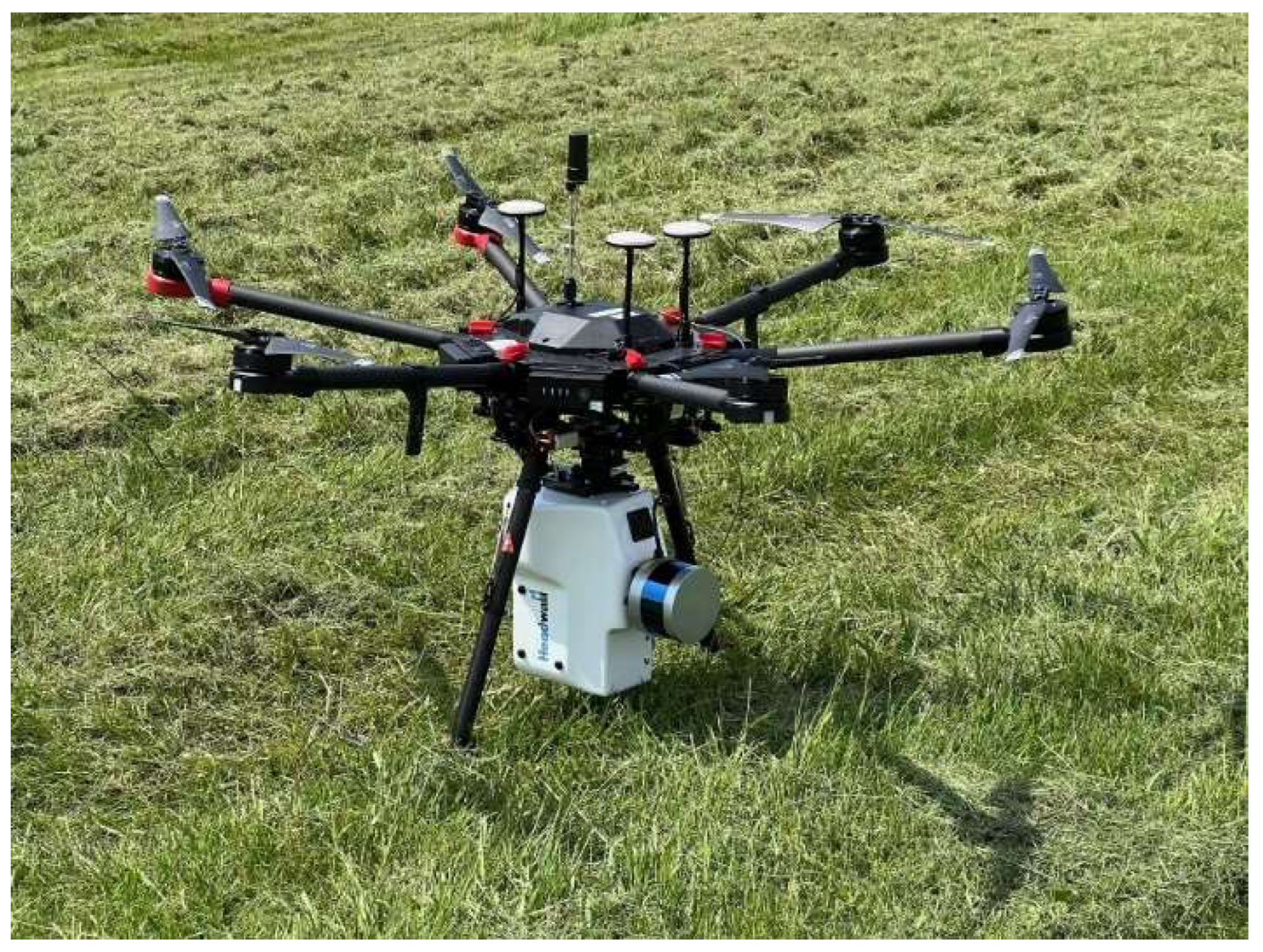
UAV-based LiDAR data were collected using a Da-Jiang Innovations (DJI) Matrice 600 Pro drone (DJI Technology Co., Shenzhen, China) equipped with a Headwall Hyperspec Co-Aligned VNIR-SWIR Imaging Sensor and a 16-channel Velodyne Lidar Puck (Headwall Photonics, Inc., Bolton, MA, USA; Velodyne Lidar, San Jose, CA, USA), shown in Figure 2. The Velodyne VLP-16 Puck LiDAR sensor, operating at a wavelength of 903 nm, has a typical spatial accuracy of ±3 cm, depending on factors such as flight altitude, surface reflectivity, and GPS/IMU quality. Flight planning was conducted using UgCS Software version 5.0 (SPH Engineering, Riga, Latvia) before the initial flight. The mission was designed to cover the study areas where sample points were located, and the same flight mission was consistently executed on all flight dates to maintain uniformity across datasets. The Trimble SPS-585 Base Station (Trimble Inc., Westminster, United States) was employed for post-processing GPS data to ensure high positional accuracy. Before each flight, sensor adjustments and tests were performed using the Hyperspec III (version 2020; Headwall Bolton, Fitchburg, MA, USA), which also controlled data acquisition during the mission. The UAV, with a takeoff weight of 13.8 kg, was manually launched and landed, maintaining a flight altitude of 70 m and a speed range of 2.5–4 m s⁻¹ during data capture to balance data resolution, field coverage, and acquisition stability, while minimizing flight-induced shaking and ensuring consistent hyperspectral and LiDAR point cloud quality. A boustrophedonic lawnmower flight pattern was used, with parallel, alternating-direction flight lines to ensure full coverage of the study area. Only data collected during active scanning within the defined target polygon were retained for analysis. A total of eight point cloud datasets were collected in 2024.

2.2. LiDAR Data Pre-Processing

Once each data collection session was completed, the base data from the Trimble SPS-585 Base Station can be utilized as a reference point to enhance the accuracy of positioning data obtained by GPS receivers. The High-Performance GPS data, which are timestamped in Coordinated Universal Time (UTC), and the base data were imported into the POSPac to create the post-processed Smoothed Best Estimate of Trajectory (SBET) file. With the SBET file in conjunction with the LiDAR returns data, the Headwall software LiDAR Tools III (version 2020) created the LiDAR LASer (LAS) file, which is also known as Point Cloud Data. The point cloud output LAS file can be viewed in CloudCompare (Girardeau-Montaut) [31,32]; meanwhile, any isolated noise in the PCD caused by sunlight can be manually removed.

2.3. Point Cloud Data Preparation

The PCD for each field was filtered using the Statistical Outlier Removal algorithm to remove possible noise caused by sunlight [43]. For training the regression models, the PCD blocks corresponding to the sample points were segmented from the original dataset. Each block was a 3D column with dimensions of 1 × 1 m in the x and y axes, matching the 1 m² area where ground truth height measurements were recorded. These segmented blocks, specifically located at the sample points, were paired with their corresponding measured heights for training. For the deep learning PointCNN method, a sufficiently large and diverse training dataset was required. To achieve this, 30% of the total area of the original PCD for the entire field was randomly selected and manually labeled. This manually labeled subset served as the input for training the PointCNN model, enabling it to accurately learn and predict crop canopy height. Figure 3 summarizes the methodological framework in a flowchart.

2.4. Machine Learning Regression Modeling

Machine learning models have proven effective in leveraging the complex relationships between LiDAR-derived metrics and plant canopy characteristics [23,44]. These models can analyze large datasets, uncovering non-linear patterns that traditional statistical methods may overlook. In this study, Random Forest Regression (RFR) and Support Vector Regression (SVR) were implemented in Python 3 using scikit-learn to model the relationship between LiDAR-derived metrics and crop canopy height.

2.4.1. Random Forest Regression

RFR is an ensemble learning method that reduces variance and enhances model robustness by combining independent decision trees generated from multiple data subsets through sampling with replacement, a technique known as bagging. At each split in a tree, a random subset of features is considered, ensuring diverse tree structures. RFR is particularly well-suited for handling high-dimensional data and mitigating overfitting by averaging for regression, making it ideal for processing diverse LiDAR metrics.

2.4.2. Support Vector Regression

SVR is a machine learning method for regression tasks that works by finding the best-fit line or hyperplane in a high-dimensional space. It minimizes error while allowing a margin of tolerance (ε) around the true values. The key data points influencing this hyperplane, known as support vectors, lie closest to or outside the tolerance margin and are identified through an optimization process during training. By focusing only on these critical points, SVR achieves efficiency and reduces the risk of overfitting. SVR effectively handles both linear and non-linear relationships by using kernel functions. This flexibility makes it a powerful tool for capturing complex patterns in data, including relationships between LiDAR-derived metrics and crop canopy height. In this study, the linear kernel and radial basis function (RBF) kernel were utilized to model the relationship between LiDAR-derived metrics and crop height. Two key hyperparameters were tuned: C, which controls the trade-off between minimizing training errors and maintaining a smooth decision boundary, and σ, the kernel parameter for the RBF kernel, which determines the influence of individual data points on the model [45,46].

For each 3D column, commonly applied LiDAR-derived metrics were calculated using all points within the column [23,35,44]. To compute the Laser Intercept Index (LII), the bottom 10% of points were classified as ground points, while the remaining points were classified as non-ground points. These metrics served as input features for training machine learning regressions. A detailed list of the metrics used during the training process is presented in

Table 2. The 19 Feature Variables used in RFR and SVR.

LiDAR-Derived Metrics	Description
Height_Max	Maximum height of the point cloud.
Height_Mean	Average height of the point.
Height_Std	Standard deviation of height values.
Height_Skewness	Measures the asymmetry of the height distribution.
Height_Kurtosis	Quantifies peakedness or flatness of the height distribution.
Height_Coefficient_of_Variation [47]	Normalized variability, calculated as ratio of standard deviation to mean height.
Canopy Relief Ratio (CRR) [48]	CRR = (Height_Mean − Height_Min)/ (Height_Max − Height_Min)
Laser Intercept Index (LII) [49]	LII = Nv/(Nv + Ng), where Nv and Ng are numbers of vegetation points and ground points separately.
P50–P99	Percentile heights from 50th to 99th percentile (P50, P60, P70, P80, P85, P88, P90, P92, P95, P98, P99).

.

2.5. Ground Point Classification

Ground points refer to the backscattered laser signals reflected from the bare earth surface, while non-ground points correspond to signals reflected from all non-terrain features, including buildings, vegetation, and other above-ground structures. Differentiating ground and non-ground points and generating accurate ground point classifications are essential for subsequent point cloud analyses, such as height extraction and 3D model construction. Consequently, selecting an appropriate ground point classification method is a critical processing step. In this study, two widely recognized approaches, the CSF algorithm and the deep learning-based PointCNN model, are utilized to classify ground points from UAV-based LiDAR PCD. Both methods demonstrated high overall accuracy and strong transferability in ground classification when applied to UAV-LiDAR point clouds collected from agricultural fields [18,43].

2.5.1. CSF

The Cloth Simulation Filter (CSF) algorithm is a widely recognized method for filtering ground points in PCD and has been extensively implemented in various software applications, including CloudCompare v2.13.1. When applied to point cloud datasets, the CSF algorithm inverts the point cloud and simulates the placement of a flexible cloth above it. Under the influence of gravity, the cloth deforms and conforms to the underlying terrain, mimicking natural surface interactions. The final shape of the deformed cloth, determined by the interactions between its nodes and the corresponding LiDAR points, serves as a reference surface. This surface is then used to classify the original point cloud into ground and non-ground points, facilitating further DTM extraction [39].

2.5.2. PointCNN

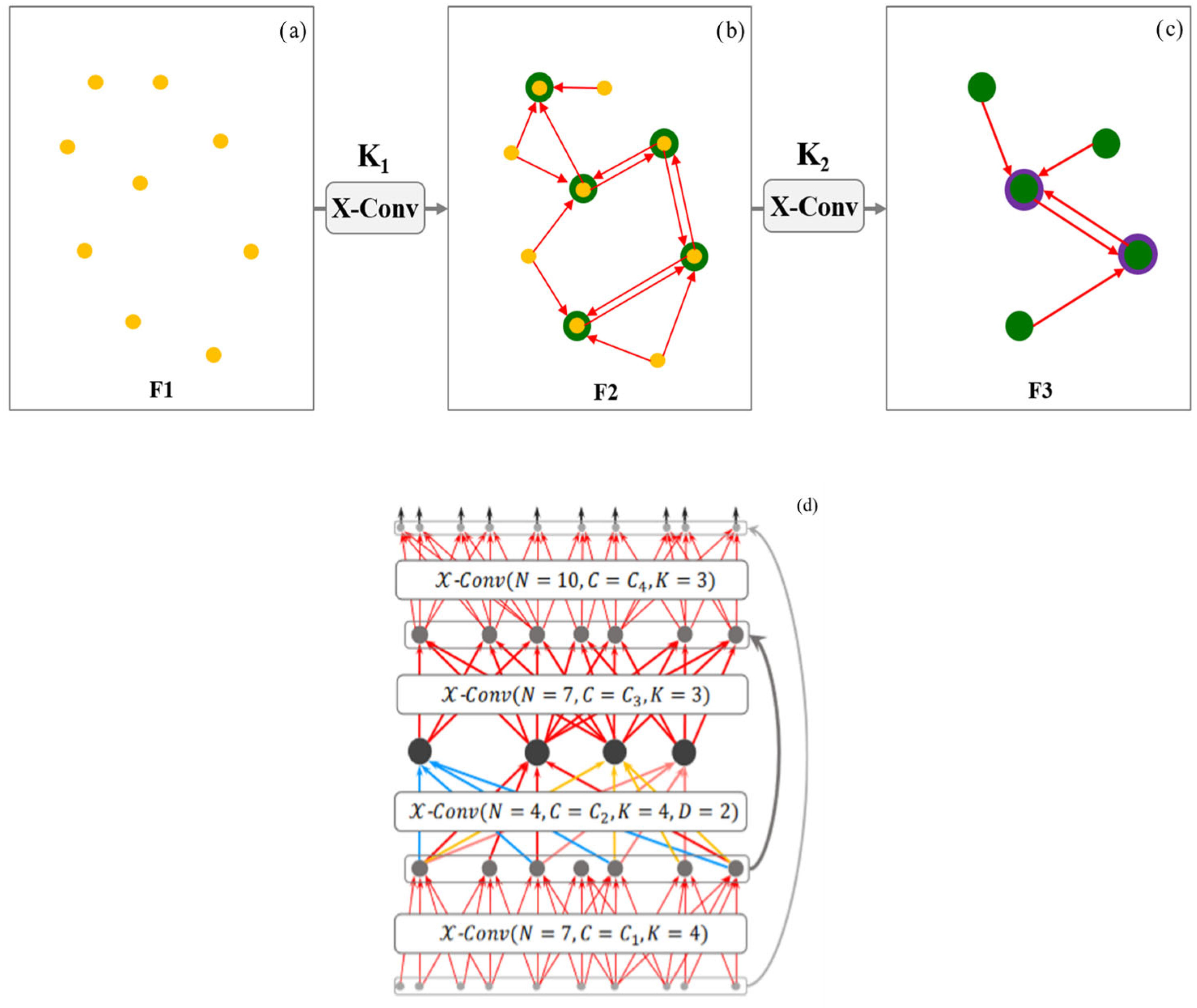
In 2018, Li et al. (2018) [40] introduced the PointCNN model for feature learning from point clouds. The PointCNN model is a generalization of typical Convolutional Neural Networks (CNNs), it adopts a convolutional-based approach in a hierarchical manner to learn on irregular PCD. The core of PointCNN is the transformation. The X-Conv recursively operates in local regions, learns a transformation matrix that permutes the input neighborhood points of each centroid into a more canonical form and weighs the features of the points before they are processed by a typical convolution. The application of convolution on the X-transformed features greatly enhances the utilization of convolution kernels and enhances the ability of convolution operations to extract features from unordered PCD [18,40,50,51,52].

In Figure 4a–c, the transformation of dense point clouds into a reduced set of points with learned information is illustrated. At each hierarchical convolution step, the X-Conv operation is applied to aggregate information from the point neighborhoods into a smaller number of representative points (9 → 5 → 2), each containing richer information. Figure 4d depicts the PointCNN architecture for segmentation. The X-Conv operator not only transforms the input points (with or without features) into fewer representation points but also propagates global information into high-resolution predictions. In Figure 4d, F denotes the feature map, N denotes the output representative point number, C represents feature dimensionality, ${\mathrm{K}}_i$ is the number of neighboring points for each representative point or ${\mathrm{K}}_i$ nearest neighbors, and D is the X-Conv dilation rate [18,40,50].

The PointCNN model can be implemented through Python scripts or directly within ArcGIS Pro (Environmental Systems Research Institute, Inc., Redlands, CA, USA). In this study, the PointCNN model was applied using ArcGIS Pro’s deep learning geoprocessing tools. The Prepare Point Cloud Training Data tool organizes the input datasets into a structured format suitable for training and validating the classification model. The prepared file is then utilized by the Train Point Cloud Classification Model tool to develop the classification models. Separate models were trained for each point cloud dataset collected on individual flight dates, while combined models incorporating multiple datasets were also trained for comparison. The PointCNN model architecture was employed for training, using the X, Y, and Z attributes of each point as input features. The model selection criteria were based on Validation Loss, where the model with the lowest entropy loss on the validation data was selected. Training parameters included a maximum of 11 epochs, determined from prior experience, and the implementation of the One Cycle Learning Rate strategy. This strategy dynamically adjusted the learning rate during each epoch, following the Fast AI 1-cycle technique. The batch size was set to its default value of 2. At the end of each training session, the model was saved in a Deep Learning Package [53].

2.6. Percentile-Based Method and Dual-Range Averaging Method

2.6.1. Percentile-Based Method

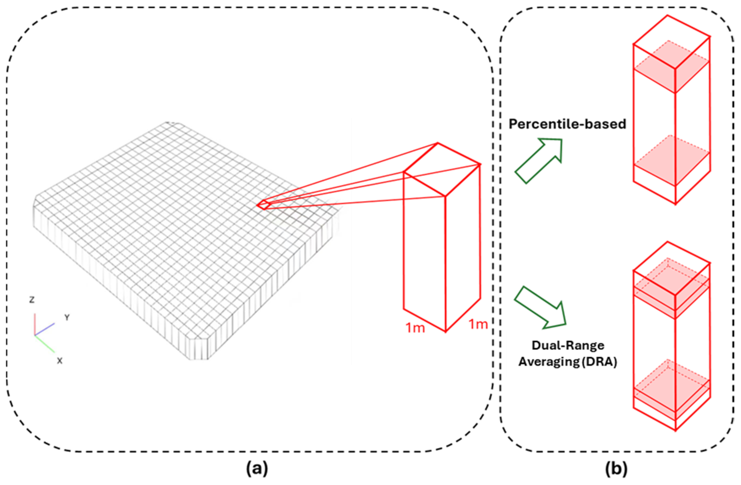
The percentile-based method is a statistical approach that estimates canopy height from the distribution of point elevations within a point cloud. To account for spatial variability, the PCD is divided into 1 × 1 m 3D columns (Figure 5a), enabling localized analysis. Within each column, canopy height is calculated as the difference between an upper and a lower percentile. As illustrated in Figure 5b, upper percentiles are selected from 80% to 100% in 0.5% increments to represent the canopy surface, while lower percentiles are selected from 0% to 20% in 0.5% increments to approximate the ground surface. This approach reduces the influence of noise and outliers by focusing on representative portions of the elevation distribution.

2.6.2. Dual-Range Averaging Method

The Dual-Range Averaging (DRA) method follows the same initial step as the percentile method, with the PCD divided into 1 × 1 m 3D columns to account for spatial variability. Within each column, various top and bottom elevation ranges are systematically tested to identify the optimal combination for accurate height estimation. The upper boundary is defined by selecting a starting percentile between 80% and 100%, in 1% increments, with an ending percentile extending at least 2% higher, up to 100%, using 2% increments. The lower boundary is established by selecting a starting percentile from 20% down to 0%, in 2% increments, with the ending percentile at least 2% lower than the starting point. The canopy height is then estimated by calculating the difference between the average height of points within the top range and the average height of points within the bottom range. This averaging approach minimizes the impact of outliers and ensures a stable, representative estimate of canopy height, particularly in areas with irregular elevation patterns.

Unlike the percentile-based method, which relies on predefined cutoffs (e.g., the 98th percentile), the DRA method simultaneously optimizes both upper and lower range thresholds within each 3D column. This dual-threshold strategy improves robustness by accounting for structural variability and uneven point density, providing a more representative characterization of canopy structure under diverse field conditions. It is particularly useful for densely planted crops with homogeneous canopies, such as winter wheat, where a single high percentile may oversimplify the canopy surface. Because ground-truth canopy heights in this study were averaged from six physical measurements per block, incorporating a broader set of canopy points ensures more consistent and comparable estimates. Furthermore, in dense canopy fields where ground points are often incompletely captured, the flexibility to adjust both top and bottom thresholds helps mitigate errors and enhances accuracy.

To determine the optimal parameter combinations for both methods, the Pareto efficiency score approach was applied, following the methodology outlined by Ten Harkel et al. (2019) [29]. Performance was evaluated independently for each collection date using the metrics described in Section 2.7, thereby accounting for temporal variability in canopy structure.

2.7. Accuracy Assessment

To assess the performance of different height estimation methods, three evaluation metrics were used: root mean square error (RMSE), mean absolute error (MAE), and coefficient of determination (R²). RMSE and MAE measure the magnitude of estimation errors, with RMSE being more sensitive to larger deviations, while MAE reflects the average error. R² evaluates the strength of the correlation between estimated and measured canopy heights, indicating how well the model captures variability in the data. The equations for these metrics are as follows:

$$RMSE=\sqrt{{\displaystyle \frac{{\sum }_{i=1}^n{\left(y_i-{\hat{\mathrm{y}}}_i\right)}^2}{n}}}$$

(1)

$$MAE={\displaystyle \frac{{\sum }_{i=1}^n\left|y_i-{\hat{\mathrm{y}}}_i\right|}{n}}$$

(2)

$$R^2=1-{\displaystyle \frac{{\sum }_{i=1}^n{\left(y_i-{\hat{\mathrm{y}}}_i\right)}^2}{{\sum }_{i=1}^n{\left(y_i-\overline{\mathrm{y}}\right)}^2}}$$

(3)

where yᵢ represents the observed value for the $i$-th observation, while ŷᵢ denotes the corresponding predicted value. The term ȳ refers to the mean of the observed values, and n is the total number of observations. The index $i$ serves as the summation index, increasing from 1 to n.

For machine learning models, performance was assessed using 100 random splits of the ground-truth samples, with each split divided into 70% training and 30% validation subsets. Validation samples were entirely excluded from training. Repeated cross-validation was employed to maximize the use of available data. The reported RMSE, MAE, and R² values represent the average across all iterations, minimizing partitioning bias and providing a more reliable assessment of model performance.

3. Results

3.1. Machine Learning Regression Modeling

The performance of RFR and SVR using both RBF and linear kernels was evaluated for crop height estimation across three crop types: soybean, corn, and winter wheat. A total of 19 LiDAR-derived variables were used as input features, including height-related metrics, the LII, and percentile heights (P50–P99). Model performance was assessed using the coefficient of determination, RMSE and significance level (p-value). For each crop type, only the results from the SVR kernel function that yielded the best performance are presented, with the linear kernel selected for corn and the RBF kernel used for soybean and wheat. The results are summarized in the corresponding tables.

The results for corn height estimation are presented in

Table 3. Training and validation statistics for corn: analysis by date and modeling approach (RFR and SVR with linear kernel) using 19 LiDAR-derived variables as input features. n represents the number of data entries for each dataset.

Date	Model	(n)	Training			Validation
			R2	p-Value	RMSE (m)	R2	p-Value	RMSE (m)
June 12	RFR	32	0.83	<0.05	0.014	−0.6	NS	0.039
	SVR	32	0.05	NS	0.033	−0.43	NS	0.037
July 4	RFR	32	0.87	<0.01	0.058	−0.13	NS	0.155
	SVR	32	0.23	NS	0.141	−0.07	NS	0.151
June 12, July 4	RFR	64	0.99	<0.001	0.066	0.93	<0.001	0.164
	SVR	64	0.97	<0.001	0.106	0.95	<0.001	0.137

. The SVR model using a linear kernel outperformed the RBF kernel and, in some cases, surpassed the RFR. The RFR showed strong training performance, particularly on July 4, where it achieved a training R² of 0.87 and an RMSE of 0.058 m. However, validation results for single-date datasets were weak, with non-significant R² values for both models. The best validation performance was achieved with the combined June 12 and July 4 datasets, where the RFR reached a validation R² of 0.93 and an RMSE of 0.164 m. The SVR model performed even better with the linear kernel, achieving a validation R² of 0.95 and an RMSE of 0.137 m. These results suggest that the linear kernel is more effective for corn height estimation, particularly when utilizing multi-temporal data.

The performance of RFR and SVR models for soybean height estimation is summarized in

Table 4. Training and validation statistics for soybean: analysis by date and modeling approach (RFR and SVR with RBF kernel) using 19 LiDAR-derived variables as input features. n represents the number of data entries for each dataset.

Date	Model	(n)	Training			Validation
			R2	p-Value	RMSE (m)	R2	p-Value	RMSE (m)
July 4	RFR	31	0.83	<0.05	0.01	−0.35	NS	0.026
	SVR	31	−0.05	NS	0.023	−0.2	NS	0.025
July 19	RFR	31	0.93	<0.001	0.014	0.45	NS	0.037
	SVR	31	0.7	NS	0.03	0.34	NS	0.042
July 26	RFR	31	0.93	<0.001	0.021	0.49	NS	0.055
	SVR	31	0.82	<0.05	0.032	0.4	NS	0.059
July 4, 19	RFR	62	0.96	<0.001	0.023	0.74	<0.001	0.059
	SVR	62	0.81	<0.001	0.053	0.7	<0.001	0.066
July 4, 26	RFR	62	0.98	<0.001	0.024	0.89	<0.001	0.057
	SVR	62	0.91	<0.001	0.054	0.86	<0.001	0.066
July 19, 26	RFR	62	0.96	<0.001	0.018	0.68	<0.001	0.049
	SVR	62	0.82	<0.001	0.037	0.65	<0.001	0.052
July 4, 19, 26	RFR	93	0.98	<0.001	0.024	0.83	<0.001	0.061
	SVR	93	0.87	<0.001	0.055	0.81	<0.001	0.065

. The RFR consistently outperformed the SVR model across all datasets. When trained on separate date, referred to as the separate-date model, the RFR demonstrated strong predictive performance, achieving the highest training R² of 0.93 on July 19, with an RMSE of 0.014 m. However, validation performance for separate-date models was generally weak, with non-significant R² values, indicating limited generalizability. The separate-date SVR model, using the RBF kernel, showed lower performance than the RFR, with several instances of negative R² values. Performance improved substantially when combining datasets from multiple dates. When trained on the full dataset from all three dates (July 4, 19, and 26), the RFR achieved a validation R² of 0.83 and an RMSE of 0.061 m. The best results were obtained when using the datasets from July 4 and 26, with the RFR reaching a validation R² of 0.89 and an RMSE of 0.057 m. The SVR model also improved under the same conditions, achieving a validation R² of 0.86 and an RMSE of 0.066 m.

The performance of the RFR and SVR models for winter wheat height estimation is presented in

Table 5. Training and validation statistics for winter wheat: analysis by date and modeling approach (RFR and SVR with RBF kernel) using 19 LiDAR-derived variables as input features. n represents the number of data entries for each dataset.

Date	Model	(n)	Training			Validation
			R2	p-Value	RMSE (m)	R2	p-Value	RMSE (m)
May 2	RFR	40	0.92	<0.001	0.056	0.4	NS	0.12
	SVR	40	0.7	<0.05	0.11	0.35	NS	0.129
May 16	RFR	40	0.84	<0.001	0.013	−0.28	NS	0.029
	SVR	40	0.09	NS	0.031	−0.28	NS	0.029
May 24	RFR	40	0.86	<0.001	0.01	−0.1	NS	0.02
	SVR	40	0.04	NS	0.026	−0.16	NS	0.021
May 2, 16	RFR	80	0.91	<0.001	0.049	0.37	<0.05	0.109
	SVR	80	0.65	<0.001	0.099	0.36	NS	0.106
May 2, 24	RFR	80	0.92	<0.001	0.055	0.66	<0.001	0.08
	SVR	80	0.85	<0.001	0.075	0.63	<0.001	0.091
May 16, 24	RFR	80	0.87	<0.001	0.027	0.05	NS	0.063
	SVR	80	0.24	NS	0.066	0.07	NS	0.063
May 2, 16, 24	RFR	120	0.92	<0.001	0.049	0.58	<0.001	0.082
	SVR	120	0.76	<0.001	0.082	0.52	<0.001	0.093

. The SVR model was evaluated using the RBF kernel, while the RFR consistently outperformed SVR across all metrics. The RFR demonstrated strong training performance, with the highest R² of 0.92 observed on the combined May 2, 16 and 24 datasets. The best validation result for RFR was achieved using the combined May 2 and May 24 datasets, yielding a validation R² of 0.66 and an RMSE of 0.080 m. The SVR model showed improvements when trained on combined datasets but remained less effective than the RFR across all metrics.

Across all crop types and years, the RFR consistently outperformed the SVR model in terms of R², RMSE, and significance level, regardless of the kernel used for SVR. The choice of SVR kernel function was crop-dependent. The linear kernel performed best for corn, while the RBF kernel yielded superior results for soybean and wheat. It is important to note that although the single-date models exhibited strong training performance, their validation results were generally poor, with some yielding low or even negative R² values. This can be attributed to the relatively high number of features (19 LiDAR-derived metrics) compared to the limited sample sizes (32, 31, and 40 observations), which increases the likelihood of overfitting. As Babyak (2004) [54] notes, models with many predictors relative to sample size may fit patterns unique to the sample that do not represent true underlying relationships. Moreover, the narrow range of measured canopy heights within each single-date dataset likely limited the variability of the response variable, further constraining the regression model’s ability to generalize. These factors collectively explain the discrepancy between strong training fits and poor validation performance observed in the performance of RFR and SVR models. Thus, incorporating multi-temporal data effectively mitigated these issues, significantly improving model robustness and estimation accuracy, with the highest validation R² values observed when training on combined datasets.

3.2. Ground Point Classification and Canopy Height Estimation

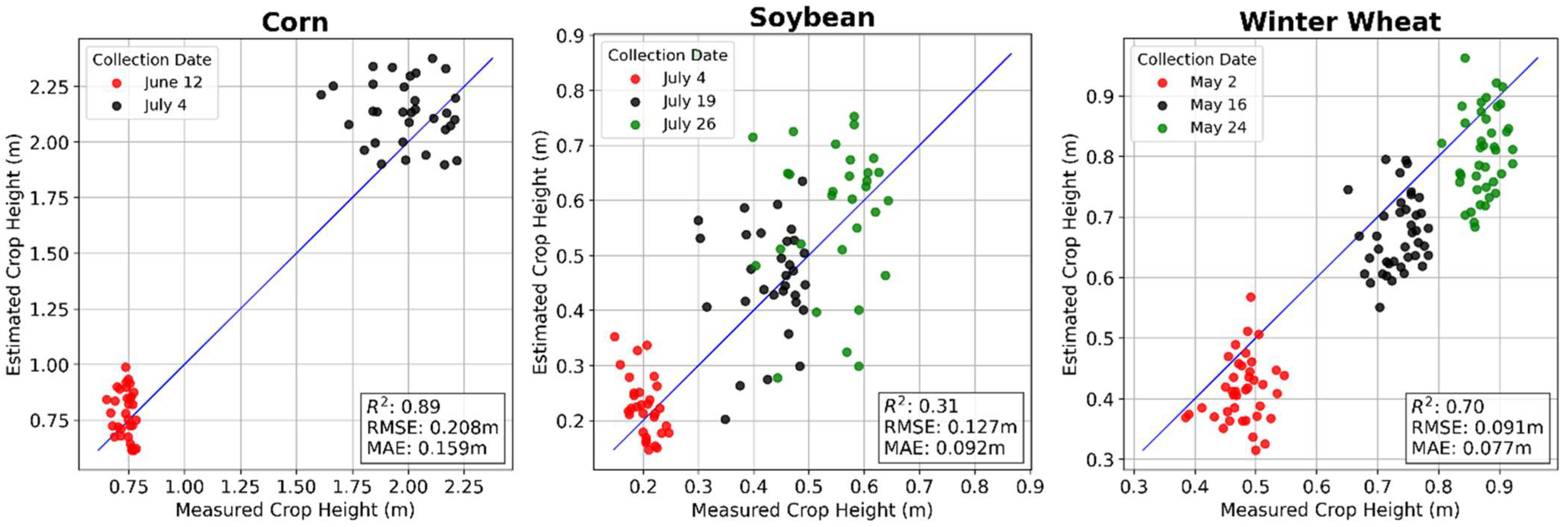
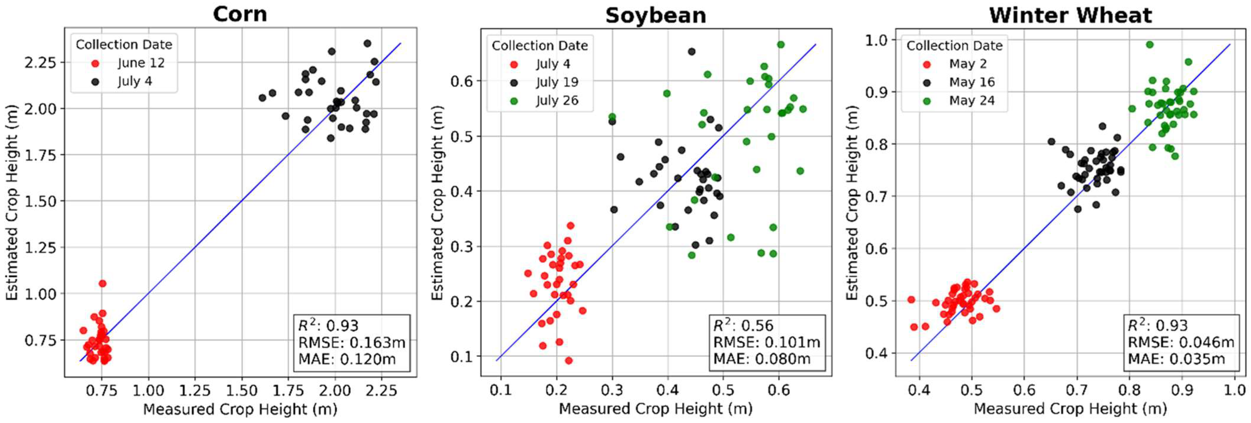
For height estimation using both ground classification methods, the ground points classified by either the CSF or PointCNN method were used to generate a DTM. This was achieved by selecting a certain percentage of the points within each 1 × 1 m 3D column and computing their average. The DSM was generated using the PCD for the entire field before classification, where the top percentage of points within each 3D column was selected and averaged to represent the upper canopy surface. Finally, crop height was estimated using the CHM, calculated as CHM = DSM − DTM [22,55]. Two approaches were used to develop the PointCNN model for ground classification. In the first approach, separate models were built for each date using only the dataset from that specific date, referred to as the separate-date model. This allowed the model to learn crop and environmental characteristics specific to each time point. In the second approach, a progressive training strategy was employed. A single model, referred to as the all-date model, was initially developed using data from the earliest date and then incrementally refined with data from subsequent dates. This approach enabled the model to retain previously learned features while adapting to new growth conditions, enhancing its ability to classify ground points across different crop stages. The performance of the CSF algorithm and the PointCNN deep learning model for ground classification was evaluated in terms of their impact on crop height estimation across corn, soybean, and winter wheat for the 2024 growing season. The evaluation results are summarized in Figure 6 and Figure 7. Regarding the PointCNN results presented in Figure 7, the separate-date model was selected for corn, as the all-date model did not produce meaningful results. In contrast, for soybean and winter wheat, the all-dates model was used, as it demonstrated comparable or superior performance to the separate-date model.

For corn, the CSF method resulted in an RMSE of 0.208 m, an R² of 0.89, and an MAE of 0.159 m. In comparison, the separate-date PointCNN model achieved a lower RMSE of 0.163 m, a higher R² of 0.93, and a reduced MAE of 0.120 m. This indicates that PointCNN provided more accurate ground classification and subsequently improved crop height estimation. However, the all-date PointCNN model failed to generate meaningful results, suggesting that pooling datasets across different growth stages may introduce inconsistencies that reduce model effectiveness, particularly when corn undergoes rapid growth and significant height and morphological changes within a short period.

For soybean, the all-date PointCNN model performed slightly better than both the separate-date PointCNN model and the CSF method. The all-date PointCNN model yielded an RMSE of 0.101 m, an R² of 0.56 and an MAE of 0.080 m. The separate-date PointCNN model produced similar results, with an RMSE of 0.104 m and an R² of 0.54. The CSF method, however, had a considerably lower R² of 0.31 and a higher RMSE of 0.127 m, indicating that it was less effective for soybean ground classification.

For winter wheat, the PointCNN model provided the most accurate height estimates. The all-date model PointCNN achieved an RMSE of 0.046 m, an R² of 0.93, and an MAE of 0.035 m. The separate-date PointCNN model produced similar results, with an RMSE of 0.047 m and an R² of 0.92. The CSF method, in contrast, exhibited lower performance with an RMSE of 0.091 m, an R² of 0.70, and an MAE of 0.077 m. The results suggest that the deep learning-based PointCNN classification method is more effective in delineating ground points for winter wheat canopy height estimation.

Across all crop types, PointCNN outperformed the CSF method in terms of lower RMSE, higher R², and reduced MAE, demonstrating its ability to more accurately classify ground points and improve canopy height estimation. The advantage of separate-date training data was particularly evident for corn, where the all-date PointCNN model failed to generate reliable results. For soybean and wheat, however, the differences between the all-dates and separate-date PointCNN models were minimal, suggesting that for these crops, the model generalizes well across different dates. Overall, these findings indicate that deep learning-based ground classification methods provide superior accuracy compared to traditional filtering algorithms like CSF, particularly when applied with appropriate training data.

3.3. Percentile-Based Method and Dual-Range Averaging Method

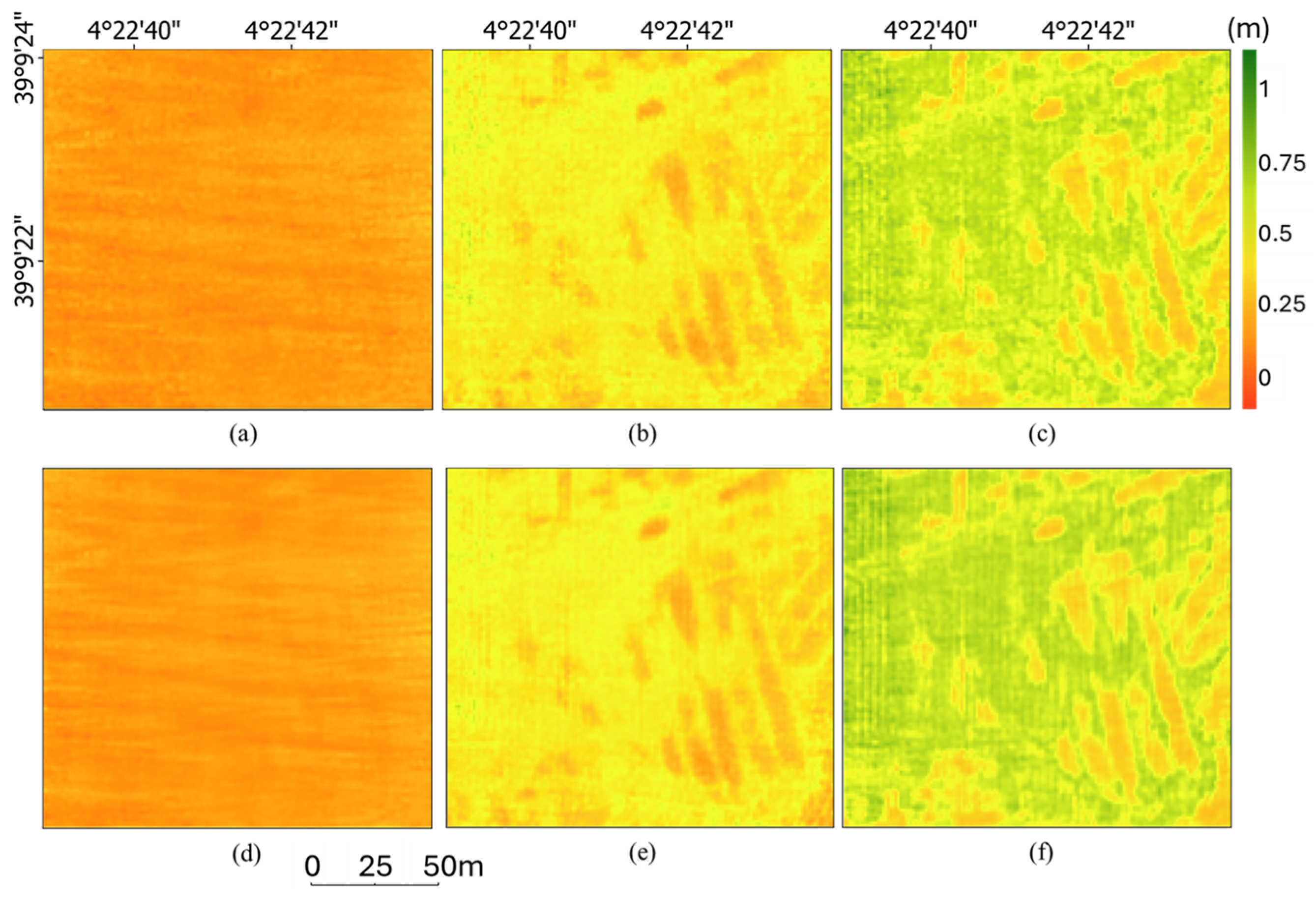
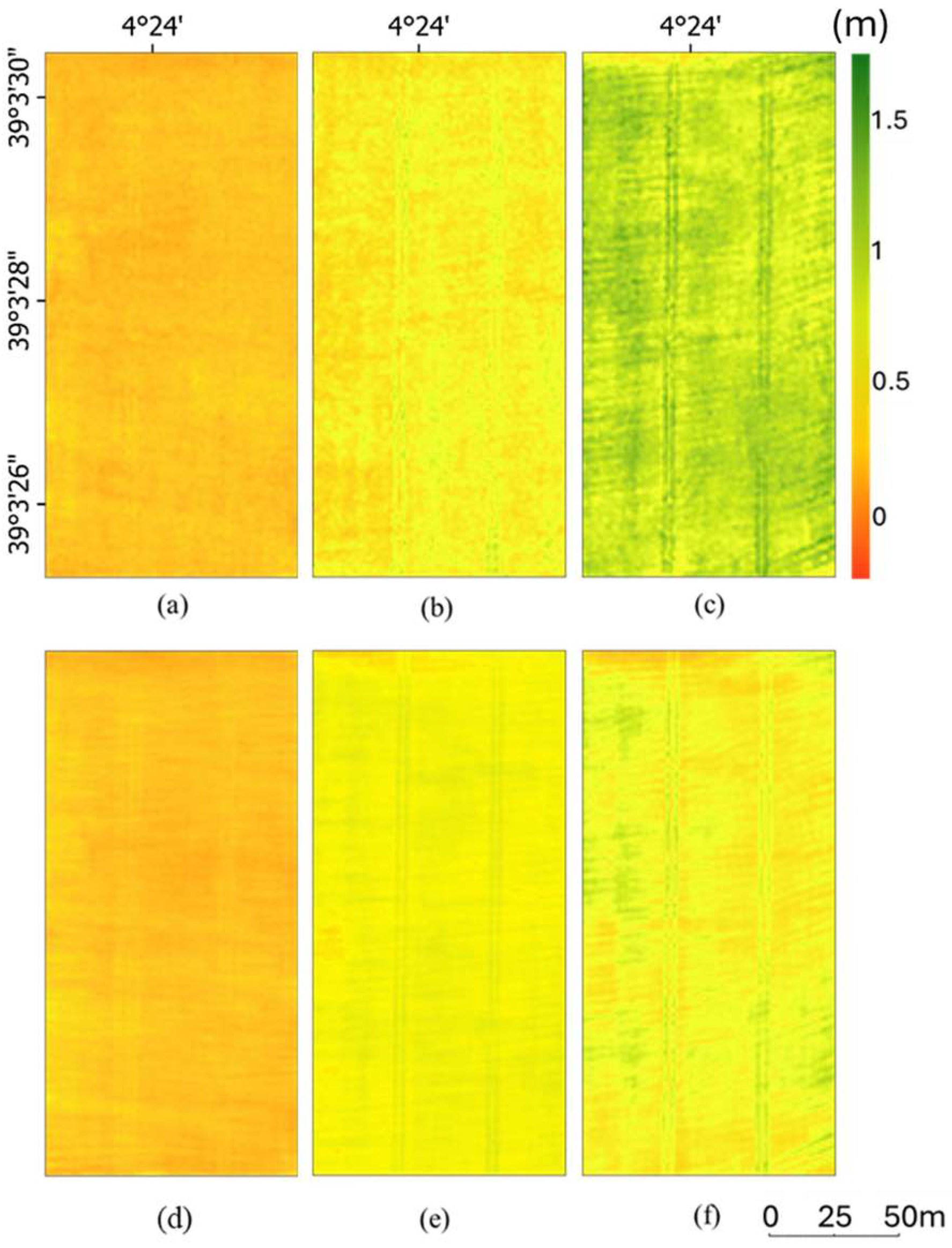
The performance of the percentile-based method and Dual-Range Averaging (DRA) method for crop height estimation was evaluated across three crop types: corn, soybean, and wheat for the 2024 growing season. Model performance was assessed using RMSE, R², and MAE. Two dataset generation strategies for finding the best top-bottom boundary combination were compared: using all dates’ datasets combined and using each corresponding date’s dataset separately. For each crop type, the performance of both methods, along with the corresponding optimal percentile or range values, is summarized in

Table 6. Statistics Performance of Percentile-Based and DRA Methods for Crop Height Estimation.

Crop Type	Dataset Generation Strategy	Percentile Method			Range Method
		R2	RMSE (m)	MAE (m)	R2	RMSE (m)	MAE (m)
Corn	All Dates	0.93	0.175	0.129	0.9	0.216	0.174
	Separate Date	0.93	0.171	0.124	0.92	0.189	0.143
Soybean	All Dates	0.66	0.08	0.071	0.66	0.08	0.072
	Separate Date	0.91	0.037	0.027	0.93	0.032	0.024
Winter Wheat	All Dates	0.29	0.146	0.121	0.33	0.145	0.122
	Separate Date	0.86	0.066	0.05	0.91	0.055	0.038

and

Table 7. Percentile and DRA Thresholds for Each Crop Type Height Estimation Using Corresponding Date-Specific Datasets.

Crop Type	Date	Percentile (%)		Range (%)
		Top	Bottom	Top	Bottom
Corn	June 12	91.5	0.5	91–93	0–2
	July 4	91.5	0	98–100	0–2
Soybean	July 4	82	20	81–83	18–20
	July 19	87.5	5	80–82	0–6
	July 26	83	3.5	81–85	2–4
Winter Wheat	May 2	80	2.5	85–97	10–14
	May 16	86.5	0	86–100	0–2
	May 24	97	0.5	94–100	0–2

and shown in the crop height maps (Figure 8, Figure 9 and Figure 10). For corn, the percentile method using the corresponding date-specific dataset outperformed the DRA method. This approach resulted in an RMSE of 0.171 m, an R² of 0.93, and an MAE of 0.124 m. The optimal top and bottom percentile thresholds varied by date. For the June 12 point cloud dataset, the best thresholds were the top 91.5% and bottom 0.5%, while for July 4, the top 91.5% and bottom 0% provided the most accurate results. For soybean, the DRA method using corresponding date-specific datasets produced the most accurate results, with an RMSE of 0.032 m, an R² of 0.93, and an MAE of 0.024 m. The optimal top and bottom range thresholds varied by date. For the point cloud dataset collected on July 4, the best-performing range was between the top 81–83% and the bottom 18–20%. For July 19, the range was 80–82% at the top and 0–6% at the bottom, while for July 26, the most effective range was 81–85% at the top and 2–4% at the bottom. For wheat, the DRA method using corresponding date-specific datasets yielded the best performance, with an RMSE of 0.055 m, an R² of 0.91, and an MAE of 0.038 m. The optimal top and bottom range thresholds varied across dates. For the May 2 dataset, the most accurate results were obtained using a top range of 85–97% and a bottom range of 10–14%. For May 16, the optimal range was 86–100% at the top and 0–2% at the bottom, while for May 24, the best-performing range was 94–100% at the top and 0–2% at the bottom. Across all three crop types, generating percentiles or ranges from corresponding date-specific datasets consistently improved height estimation performance compared to using combined data from all dates.

4. Discussion

4.1. Performance Comparison of Crop Height Estimation Methods

In this study, three crop height estimation approaches, including machine learning regression models, ground point classification techniques, percentile-based method and Dual-Range Averaging (DRA) method, were evaluated and compared across three crop types: corn, soybean, and winter wheat. Among all tested methods, the DRA method had the best performance, with an average R² of 0.92 and an average RMSE of 0.092 m across all crop types. In contrast, the CSF ground point classification method yielded the lowest accuracy, with an average R² of 0.64 and RMSE of 0.142 m. The limited performance of the CSF method was particularly evident in soybean fields. Compared to winter wheat, which is densely planted with narrow row spacing of around 10 cm in width, soybean and corn fields have wider row spacing, approximately 70 cm and 75 cm, respectively, according to our ground truth data collection. In early growth stages, before full canopy closure, the wider spacing allows greater ground visibility, enabling more laser pulses to reach the ground and collect more ground points. Despite this, soybean fields present unique challenges. The average height of soybean plants across the three growth stages ranged from 0.20 m to 0.54 m. Additionally, the undulating terrain commonly found in many agricultural fields, including soybean fields, further complicated the classification of ground points. The relatively short plant height, combined with the ridge bed planting pattern, makes it more difficult to distinguish soil ground from vegetation in the LiDAR point clouds. As a result, both the CSF and PointCNN showed lower accuracy for ground point classification in soybean fields, which subsequently affected the accuracy of height estimation for soybean. For soybean, the DRA method was the most accurate, while for corn, the SVR model with a linear kernel function performed the best. Though the corn field has wider row spacing, allowing for some ground returns in early stages, once corn reaches full height, the broad foliage leaves and tall stalks densify the corn canopy and subsequently limit ground returns, which is a typical challenge for LiDAR-based crop monitoring [56]. Figure 11 illustrates the reduction in ground points in the corn field PCD by comparing the point clouds collected on June 12 and July 4. For winter wheat, the PointCNN deep learning model excelled in ground classification and height estimation. The homogeneous canopy structure and narrow leaves of winter wheat allowed sufficient laser penetration through the canopy, enabling the deep learning model to effectively classify ground points and vegetation points.

The relative importance of LiDAR-derived features was evaluated based on the mean decrease in impurity (MDI) from the RFR [57]. The computed importance values indicate each feature’s proportional contribution to improving model accuracy and were averaged across multiple models trained on different datasets to ensure robust estimates. According to the results shown in Figure 12, the top three most important features varied by crop type. For soybean, the most influential features were the 88th, 80th, and 90th height percentiles (P88, P80, and P90), while for winter wheat, the top features included the 95th and 92nd percentiles (P95 and P92), along with the maximum height. However, in the corn canopy height estimation, the most influential features identified by the RFR were CRR, height skewness, and height coefficient of variation, rather than traditional percentile-based metrics. This result contrasts with the results reported by Luo et al. (2021) [23], where the top three features for estimating corn and soybean canopy height were P99, maximum height, and P95, which all directly represent extreme height values. Our finding highlights the importance of structural and distributional characteristics of the LiDAR point cloud over absolute height values. One possible explanation is the temporal variation in canopy development. On June 12, the corn plants were relatively short and sparsely distributed, resulting in a higher proportion of laser pulse returns from the ground and lower canopy layers. In contrast, by July 4, the corn canopy had reached approximately 2 m in height, with increased foliage leaf density at the top and fewer laser pulse returns penetrating to the bottom of the crop or the ground. Under such conditions, percentile-based metrics may lose sensitivity to the overall height growth of corn due to the dominance of top canopy returns. In comparison, structural metrics like the Canopy Relief Ratio and statistical measures such as skewness and coefficient of variation provide a more precise representation of the vertical canopy structure, capturing informative changes in plant architecture and spatial variability. These findings suggest that in dense and vertically non-uniform crops like corn, the distribution-based LiDAR-derived metrics can be more effective than extreme height percentiles for accurately estimating crop canopy height.

Between the two ground point classification methods, PointCNN and CSF, PointCNN demonstrated superior performance in canopy height estimation, which aligns with the findings reported by Fareed et al. (2023) [18]. PointCNN achieved a higher average coefficient of determination (R² = 0.80) compared to CSF (R² = 0.64), representing an improvement of 0.16 in R². Meanwhile, PointCNN yielded a lower RMSE of 0.104 m relative to CSF with an RMSE of 0.142 m. These results show the advantage of deep learning-based point cloud classification for distinguishing ground and non-ground points in agricultural fields with homogeneous canopy structures, contributing to more accurate crop height estimation.

In the winter wheat canopy height map generated using the percentile-based method and DRA method, the tracks left by vehicles or trucks exhibit higher estimated heights compared to the surrounding crop areas. This overestimation can be attributed to the distribution and representation of ground points within the LiDAR point cloud. As vehicles traverse the field, their tires compress the soil, leaving tracks that are slightly depressed relative to the adjacent planted beds. These compacted tracks often expose more bare soil, leading to more ground points collected, and more importantly, ground points with lower elevation values than those in undisturbed crop rows. Within the 1 × 1 m 3D columns used for height extraction, the upper boundary defined by canopy points remains consistent with adjacent crop regions. However, since the lower boundary is defined by these relatively lower elevation ground points, the calculated canopy height, which is based on the difference between the top and bottom boundaries, tends to be overestimated. Consequently, pixels along the tracks appear darker on the canopy height map, reflecting an overestimation of height. This highlights a known limitation in height extraction methods that rely on vertical differencing, especially in crop fields where ground surface uniformity is disrupted.

4.2. Methodological Limitations and Practical Considerations

While this study demonstrates the effectiveness of UAV-based LiDAR for crop height estimation, several limitations should be acknowledged. First, the performance of the PointCNN deep learning model is highly dependent on the availability and quality of manually labeled training data. Preparing such datasets is time-consuming and requires careful supervision, which may limit the model’s scalability in large-scale or real-time applications [18]. In contrast, CSF provides a more automated workflow, making it advantageous in operational settings where ease of use and processing efficiency are prioritized over maximal accuracy. Second, ground classification accuracy remains a challenge, particularly in crops with low canopy height, such as soybean, where minimal elevation differences between soil and vegetation points complicate differentiation. This observation is consistent with the findings of Pun Magar et al. (2025) [24] and Fareed et al. (2023) [18], who reported similar difficulties in distinguishing ground and vegetation points in low-canopy agricultural fields. This limitation impacted the subsequent accuracy of height estimation [58]. Another constraint is the challenge of acquiring LiDAR data for bare ground prior to or immediately after seeding, which is critical for improving DTM accuracy [59,60]. Although feasible for spring-sown crops, this is generally impractical for winter wheat due to its autumn planting schedule. In such cases, growers rarely request UAV monitoring ahead of the active growing season, limiting opportunities to obtain bare ground data and thereby reducing the feasibility of precise pre-season ground modeling.

In this study, the ground truth crop canopy heights were calculated by averaging six manual measurements per block to enhance reliability and reduce sampling error. However, even with this approach, inherent variability remains due to several well-documented challenges associated with manual field measurements. Studies have shown that manual plant height measurements can exhibit considerable variation, especially during early growth stages when canopy structures are less developed. For example, replicated manual measurements of the same plants have shown low correlation and higher error early in the season, with performance improving as plants mature and canopy structure becomes more distinct. Additionally, when plot-mean heights are based on a limited number of sampled plants, variability can arise depending on plant selection, introducing further uncertainty into the ground truth data [61]. A further source of uncertainty arises from how ground elevation was handled in this study. The DTM was generated with a spatial resolution of 1 m, meaning each 1 × 1 m block was assigned a single ground elevation value. However, within each block, six manual canopy height measurements were taken at different points. Because crop fields are typically sown in furrows and have naturally uneven ground surfaces, the true ground level at each measurement point may differ slightly from the DTM’s uniform value [62]. This mismatch introduces additional errors into the canopy height calculation. Combined with natural canopy variability due to micro-environmental differences within the block, these factors mean that averaged manual measurements may not perfectly represent the true crop canopy. Such findings reinforce that small RMSE differences that are within approximately 1–3 cm between different estimation models or methods likely fall within the expected margin of measurement uncertainty and should be interpreted cautiously in terms of practical significance [61]. Therefore, when selecting the optimal method or comparing model performance, it is important not only to consider the ranking of statistical assessment but also to evaluate each method from a practical perspective, taking into account factors such as processing time, ease of use, availability, and compatibility with the existing workflow. These practical considerations are essential to ensure that the chosen method is not only accurate but also feasible and efficient for operational deployment.

5. Conclusions

This study demonstrated the potential of UAV-based LiDAR data for accurately estimating crop canopy height in corn, soybean, and winter wheat through a comparative analysis of three height estimation methodological approaches: machine learning regression modeling, ground point classification techniques, percentile-based method and newly proposed Dual-Range Averaging (DRA) method (

Table 8. Comparison of crop canopy height estimation performance across three crop types (corn, soybean, and winter wheat) and six different methods: Random Forest Regression (RFR), Support Vector Regression (SVR), Cloth Simulation Filter (CSF), PointCNN, Percentile-based method, and the newly proposed Dual-Range Averaging (DRA) method. Bold values highlight the highest R² and lowest RMSE for each row.

Crop Type	ML Regression				Ground Point Classification				Percentile		DRA
	RFR		SVR		CSF		PointCNN
	R2	RMSE (m)	R2	RMSE (m)	R2	RMSE (m)	R2	RMSE (m)	R2	RMSE (m)	R2	RMSE (m)
Corn	0.93	0.164	0.95	0.137	0.89	0.208	0.93	0.163	0.93	0.171	0.92	0.189
Soybean	0.89	0.057	0.86	0.066	0.31	0.127	0.56	0.101	0.91	0.037	0.93	0.032
Winter Wheat	0.66	0.080	0.63	0.091	0.70	0.091	0.93	0.046	0.86	0.066	0.91	0.055
Average Performance	0.83	0.100	0.81	0.098	0.64	0.142	0.81	0.103	0.90	0.091	0.92	0.092

). The findings emphasize that no single approach universally outperforms others. Instead, the optimal method varies for each crop type due to the differences in canopy structure, growth patterns, and field conditions. SVR with a linear kernel was the most effective method for corn, especially when using multi-date datasets. The DRA method performed best for soybean. For winter wheat, the PointCNN model achieved the highest accuracy with an R² of 0.93 and an RMSE of 0.046 m, aided by its uniform canopy. Overall, the DRA method delivered the best average performance across crops with an average R² of 0.92 and an average RMSE of 0.092 m. These findings highlight the importance of tailoring height estimation approaches to specific crop characteristics and demonstrate the robust potential of UAV-based LiDAR for advancing PA. Overall, this study establishes a reproducible approach for estimating crop canopy height using UAV-based LiDAR PCD. Continued improvements in classification automation, the expansion of data acquisition strategies beyond crop-specific applications to spatio-temporal generalization, and advances in model generalization will further support the adoption of LiDAR technologies in PA through the creation of standardized frameworks. By enabling accurate, efficient, and scalable crop monitoring, the integration of UAV-based LiDAR with optimized processing workflows supports site-specific management and enhances data-driven decision-making in agricultural production.

References

1. Martos, V.; Ahmad, A.; Cartujo, P.; Ordoñez, J. Ensuring Agricultural Sustainability through Remote Sensing in the Era of Agriculture 5.0. Appl. Sci. 2021, 11, 5911. [Google Scholar] [CrossRef]
2. Velten, S.; Leventon, J.; Jager, N.; Newig, J. What Is Sustainable Agriculture? A Systematic Review. Sustainability 2015, 7, 7833–7865. [Google Scholar] [CrossRef]
3. Gebbers, R.; Adamchuk, V.I. Precision Agriculture and Food Security. Science 2010, 327, 828–831. [Google Scholar] [CrossRef]
4. Khanal, S.; Fulton, J.; Shearer, S. An Overview of Current and Potential Applications of Thermal Remote Sensing in Precision Agriculture. Comput. Electron. Agric. 2017, 139, 22–32. [Google Scholar] [CrossRef]
5. Rivera, G.; Porras, R.; Florencia, R.; Sánchez-Solís, J.P. LiDAR Applications in Precision Agriculture for Cultivating Crops: A Review of Recent Advances. Comput. Electron. Agric. 2023, 207, 107737. [Google Scholar] [CrossRef]
6. Aarif K. O., M.; Alam, A.; Hotak, Y. Smart Sensor Technologies Shaping the Future of Precision Agriculture: Recent Advances and Future Outlooks. J. Sens. 2025, 2025, 2460098. [Google Scholar] [CrossRef]
7. Chang, A.; Jung, J.; Maeda, M.M.; Landivar, J. Crop Height Monitoring with Digital Imagery from Unmanned Aerial System (UAS). Comput. Electron. Agric. 2017, 141, 232–237. [Google Scholar] [CrossRef]
8. Guo, Y.; Xiao, Y.; Li, M.; Hao, F.; Zhang, X.; Sun, H.; De Beurs, K.; Fu, Y.H.; He, Y. Identifying Crop Phenology Using Maize Height Constructed from Multi-Sources Images. Int. J. Appl. Earth Obs. Geoinf. 2022, 115, 103121. [Google Scholar] [CrossRef]
9. Eitel, J.U.H.; Magney, T.S.; Vierling, L.A.; Greaves, H.E.; Zheng, G. An Automated Method to Quantify Crop Height and Calibrate Satellite-Derived Biomass Using Hypertemporal Lidar. Remote Sens. Environ. 2016, 187, 414–422. [Google Scholar] [CrossRef]
10. Anthony, D.; Elbaum, S.; Lorenz, A.; Detweiler, C. On Crop Height Estimation with UAVs. In Proceedings of the 2014 IEEE/RSJ International Conference on Intelligent Robots and Systems, Chicago, IL, USA, 14–18 September 2014; pp. 4805–4812. [Google Scholar]
11. Lefsky, M.A.; Cohen, W.B.; Parker, G.G.; Harding, D.J. Lidar Remote Sensing for Ecosystem Studies. BioScience 2002, 52, 19. [Google Scholar] [CrossRef]
12. Cecchi, G.; Pantani, L. Fluorescence Lidar Remote Sensing of Vegetation: Research Advances in Europe. In Proceedings of the Proceedings of IGARSS ’94—1994 IEEE International Geoscience and Remote Sensing Symposium, Pasadena, CA, USA, 8–12 August 1994; Volume 2, pp. 979–981. [Google Scholar]
13. Husin, N.A.; Khairunniza-Bejo, S.; Abdullah, A.F.; Kassim, M.S.M.; Ahmad, D.; Azmi, A.N.N. Application of Ground-Based LiDAR for Analysing Oil Palm Canopy Properties on the Occurrence of Basal Stem Rot (BSR) Disease. Sci. Rep. 2020, 10, 6464. [Google Scholar] [CrossRef]
14. Wu, D.; Johansen, K.; Phinn, S.; Robson, A. Suitability of Airborne and Terrestrial Laser Scanning for Mapping Tree Crop Structural Metrics for Improved Orchard Management. Remote Sens. 2020, 12, 1647. [Google Scholar] [CrossRef]
15. Wendel, A.; Underwood, J.; Walsh, K. Maturity Estimation of Mangoes Using Hyperspectral Imaging from a Ground Based Mobile Platform. Comput. Electron. Agric. 2018, 155, 298–313. [Google Scholar] [CrossRef]
16. Bai, G.; Ge, Y.; Hussain, W.; Baenziger, P.S.; Graef, G. A Multi-Sensor System for High Throughput Field Phenotyping in Soybean and Wheat Breeding. Comput. Electron. Agric. 2016, 128, 181–192. [Google Scholar] [CrossRef]
17. Walter, J.D.C.; Edwards, J.; McDonald, G.; Kuchel, H. Estimating Biomass and Canopy Height with LiDAR for Field Crop Breeding. Front. Plant Sci. 2019, 10, 1145. [Google Scholar] [CrossRef]
18. Fareed, N.; Flores, J.P.; Das, A.K. Analysis of UAS-LiDAR Ground Points Classification in Agricultural Fields Using Traditional Algorithms and PointCNN. Remote Sens. 2023, 15, 483. [Google Scholar] [CrossRef]
19. Thudi, M.; Palakurthi, R.; Schnable, J.C.; Chitikineni, A.; Dreisigacker, S.; Mace, E.; Srivastava, R.K.; Satyavathi, C.T.; Odeny, D.; Tiwari, V.K.; et al. Genomic Resources in Plant Breeding for Sustainable Agriculture. J. Plant Physiol. 2021, 257, 153351. [Google Scholar] [CrossRef]
20. Gao, M.; Yang, F.; Wei, H.; Liu, X. Individual Maize Location and Height Estimation in Field from UAV-Borne LiDAR and RGB Images. Remote Sens. 2022, 14, 2292. [Google Scholar] [CrossRef]
21. Dhami, H.; Yu, K.; Xu, T.; Zhu, Q.; Dhakal, K.; Friel, J.; Li, S.; Tokekar, P. Crop Height and Plot Estimation for Phenotyping from Unmanned Aerial Vehicles Using 3D LiDAR. In Proceedings of the 2020 IEEE/RSJ International Conference on Intelligent Robots and Systems (IROS), Las Vegas, NV, USA, 25–29 October 2020; pp. 2643–2649. [Google Scholar]
22. Zhou, L.; Gu, X.; Cheng, S.; Yang, G.; Shu, M.; Sun, Q. Analysis of Plant Height Changes of Lodged Maize Using UAV-LiDAR Data. Agriculture 2020, 10, 146. [Google Scholar] [CrossRef]
23. Luo, S.; Liu, W.; Zhang, Y.; Wang, C.; Xi, X.; Nie, S.; Ma, D.; Lin, Y.; Zhou, G. Maize and Soybean Heights Estimation from Unmanned Aerial Vehicle (UAV) LiDAR Data. Comput. Electron. Agric. 2021, 182, 106005. [Google Scholar] [CrossRef]
24. Pun Magar, L.; Sandifer, J.; Khatri, D.; Poudel, S.; Kc, S.; Gyawali, B.; Gebremedhin, M.; Chiluwal, A. Plant Height Measurement Using UAV-Based Aerial RGB and LiDAR Images in Soybean. Front. Plant Sci. 2025, 16, 1488760. [Google Scholar] [CrossRef]
25. Liu, Q.; Fu, L.; Chen, Q.; Wang, G.; Luo, P.; Sharma, R.P.; He, P.; Li, M.; Wang, M.; Duan, G. Analysis of the Spatial Differences in Canopy Height Models from UAV LiDAR and Photogrammetry. Remote Sens. 2020, 12, 2884. [Google Scholar] [CrossRef]
26. Brede, B.; Lau, A.; Bartholomeus, H.; Kooistra, L. Comparing RIEGL RiCOPTER UAV LiDAR Derived Canopy Height and DBH with Terrestrial LiDAR. Sensors 2017, 17, 2371. [Google Scholar] [CrossRef]
27. Song, Y.; Wang, J. Winter Wheat Canopy Height Extraction from UAV-Based Point Cloud Data with a Moving Cuboid Filter. Remote Sens. 2019, 11, 1239. [Google Scholar] [CrossRef]
28. Yang, W.; Wu, J.; Xu, W.; Li, H.; Li, X.; Lan, Y.; Li, Y.; Zhang, L. Comparative Evaluation of the Performance of the PTD and CSF Algorithms on UAV LiDAR Data for Dynamic Canopy Height Modeling in Densely Planted Cotton. Agronomy 2024, 14, 856. [Google Scholar] [CrossRef]
29. Ten Harkel, J.; Bartholomeus, H.; Kooistra, L. Biomass and Crop Height Estimation of Different Crops Using UAV-Based Lidar. Remote Sens. 2019, 12, 17. [Google Scholar] [CrossRef]
30. Zhang, X.; Zhang, J.; Peng, Y.; Yu, X.; Lu, L.; Liu, Y.; Song, Y.; Yin, D.; Zhao, S.; Wang, H.; et al. QTL Mapping of Maize Plant Height Based on a Population of Doubled Haploid Lines Using UAV LiDAR High-Throughput Phenotyping Data. J. Integr. Agric. 2024, in press. [CrossRef]
31. Maimaitijiang, M.; Sagan, V.; Erkbol, H.; Adrian, J.; Newcomb, M.; LeBauer, D.; Pauli, D.; Shakoor, N.; Mockler, T.C. UAV-Based Sorghum Growth Monitoring: A Comparative Analysis of Lidar and Photogrammetry. ISPRS Ann. Photogramm. Remote Sens. Spat. Inf. Sci. 2020, 3, 489–496. [Google Scholar] [CrossRef]
32. Šrollerů, A.; Potůčková, M. Evaluating the Applicability of High-Density UAV LiDAR Data for Monitoring Tundra Grassland Vegetation. Int. J. Remote Sens. 2024, 46, 42–76. [Google Scholar] [CrossRef]
33. Li, Y.; Li, C.; Cheng, Q.; Duan, F.; Zhai, W.; Li, Z.; Mao, B.; Ding, F.; Kuang, X.; Chen, Z. Estimating Maize Crop Height and Aboveground Biomass Using Multi-Source Unmanned Aerial Vehicle Remote Sensing and Optuna-Optimized Ensemble Learning Algorithms. Remote Sens. 2024, 16, 3176. [Google Scholar] [CrossRef]
34. Liu, T.; Zhu, S.; Yang, T.; Zhang, W.; Xu, Y.; Zhou, K.; Wu, W.; Zhao, Y.; Yao, Z.; Yang, G.; et al. Maize Height Estimation Using Combined Unmanned Aerial Vehicle Oblique Photography and LIDAR Canopy Dynamic Characteristics. Comput. Electron. Agric. 2024, 218, 108685. [Google Scholar] [CrossRef]
35. Hütt, C.; Bolten, A.; Hüging, H.; Bareth, G. UAV LiDAR Metrics for Monitoring Crop Height, Biomass and Nitrogen Uptake: A Case Study on a Winter Wheat Field Trial. PFG 2023, 91, 65–76. [Google Scholar] [CrossRef]
36. Madec, S.; Baret, F.; De Solan, B.; Thomas, S.; Dutartre, D.; Jezequel, S.; Hemmerlé, M.; Colombeau, G.; Comar, A. High-Throughput Phenotyping of Plant Height: Comparing Unmanned Aerial Vehicles and Ground LiDAR Estimates. Front. Plant Sci. 2017, 8, 2002. [Google Scholar] [CrossRef]
37. Monnet, J.-M.; Chanussot, J.; Berger, F. Support Vector Regression for the Estimation of Forest Stand Parameters Using Airborne Laser Scanning. IEEE Geosci. Remote Sens. Lett. 2011, 8, 580–584. [Google Scholar] [CrossRef]
38. Chen, G.; Hay, G.J.; Zhou, Y. Estimation of Forest Height, Biomass and Volume Using Support Vector Regression and Segmentation from Lidar Transects and Quickbird Imagery. In Proceedings of the 2010 18th International Conference on Geoinformatics, Beijing, China, 18–20 June 2010; pp. 1–4. [Google Scholar]
39. Zhang, W.; Qi, J.; Wan, P.; Wang, H.; Xie, D.; Wang, X.; Yan, G. An Easy-to-Use Airborne LiDAR Data Filtering Method Based on Cloth Simulation. Remote Sens. 2016, 8, 501. [Google Scholar] [CrossRef]
40. Li, Y.; Bu, R.; Sun, M.; Wu, W.; Di, X.; Chen, B. PointCNN: Convolution On X-Transformed Points. In Advances in Neural Information Processing Systems; Bengio, S., Wallach, H., Larochelle, H., Grauman, K., Cesa-Bianchi, N., Garnett, R., Eds.; Curran Associates, Inc.: Red Hook, NY, USA, 2018; Volume 31. [Google Scholar]
41. Zhang, F.; Hassanzadeh, A.; Kikkert, J.; Pethybridge, S.J.; Van Aardt, J. Comparison of UAS-Based Structure-from-Motion and LiDAR for Structural Characterization of Short Broadacre Crops. Remote Sens. 2021, 13, 3975. [Google Scholar] [CrossRef]
42. Sangjan, W.; McGee, R.J.; Sankaran, S. Optimization of UAV-Based Imaging and Image Processing Orthomosaic and Point Cloud Approaches for Estimating Biomass in a Forage Crop. Remote Sens. 2022, 14, 2396. [Google Scholar] [CrossRef]
43. Colaço, A.F.; Schaefer, M.; Bramley, R.G.V. Broadacre Mapping of Wheat Biomass Using Ground-Based LiDAR Technology. Remote Sens. 2021, 13, 3218. [Google Scholar] [CrossRef]
44. Pearse, G.D.; Watt, M.S.; Dash, J.P.; Stone, C.; Caccamo, G. Comparison of Models Describing Forest Inventory Attributes Using Standard and Voxel-Based Lidar Predictors across a Range of Pulse Densities. Int. J. Appl. Earth Obs. Geoinf. 2019, 78, 341–351. [Google Scholar] [CrossRef]
45. Kavaklioglu, K. Modeling and Prediction of Turkey’s Electricity Consumption Using Support Vector Regression. Appl. Energy 2011, 88, 368–375. [Google Scholar] [CrossRef]
46. Jin, J.; Verbeurgt, J.; De Sloover, L.; Stal, C.; Deruyter, G.; Montreuil, A.-L.; Vos, S.; De Maeyer, P.; De Wulf, A. Support Vector Regression for High-Resolution Beach Surface Moisture Estimation from Terrestrial LiDAR Intensity Data. Int. J. Appl. Earth Obs. Geoinf. 2021, 102, 102458. [Google Scholar] [CrossRef]
47. Evans, J.S.; Hudak, A.T.; Faux, R.; Smith, A.M.S. Discrete Return Lidar in Natural Resources: Recommendations for Project Planning, Data Processing, and Deliverables. Remote Sens. 2009, 1, 776–794. [Google Scholar] [CrossRef]
48. Parker, G.G.; Russ, M.E. The Canopy Surface and Stand Development: Assessing Forest Canopy Structure and Complexity with near-Surface Altimetry. For. Ecol. Manag. 2004, 189, 307–315. [Google Scholar] [CrossRef]
49. Kwak, D.-A.; Lee, W.-K.; Cho, H.-K. Estimation of Lai Using Lidar Remote Sensing in Forest. In Proceedings of the ISPRS Workshop on Laser Scanning 2007 and SilviLaser 2007, Espoo, Finland, 12–14 September 2007. [Google Scholar]
50. Zhang, J.; Zhao, X.; Chen, Z.; Lu, Z. A Review of Deep Learning-Based Semantic Segmentation for Point Cloud. IEEE Access 2019, 7, 179118–179133. [Google Scholar] [CrossRef]
51. Bello, S.A.; Yu, S.; Wang, C.; Adam, J.M.; Li, J. Review: Deep Learning on 3D Point Clouds. Remote Sens. 2020, 12, 1729. [Google Scholar] [CrossRef]
52. Hell, M.; Brandmeier, M.; Briechle, S.; Krzystek, P. Classification of Tree Species and Standing Dead Trees with Lidar Point Clouds Using Two Deep Neural Networks: PointCNN and 3DmFV-Net. PFG 2022, 90, 103–121. [Google Scholar] [CrossRef]
53. Esri Train a Deep Learning Model for Point Cloud Classification—ArcGIS Pro|Documentation. Available online: https://pro.arcgis.com/en/pro-app/latest/help/data/las-dataset/train-a-point-cloud-model-with-deep-learning.htm (accessed on 10 April 2025).
54. Babyak, M.A. What You See May Not Be What You Get: A Brief, Nontechnical Introduction to Overfitting in Regression-Type Models. Biopsychosoc. Sci. Med. 2004, 66, 411–421. [Google Scholar]
55. Cui, Y.; Zhao, K.; Fan, W.; Xu, X. Retrieving Crop Fractional Cover and LAI Based on Airborne Lidar Data. Natl. Remote Sens. Bull. 2011, 15, 1276–1288. [Google Scholar] [CrossRef]
56. Zhou, X.; Xing, M.; He, B.; Wang, J.; Song, Y.; Shang, J.; Liao, C.; Xu, M.; Ni, X. A Ground Point Fitting Method for Winter Wheat Height Estimation Using UAV-Based SfM Point Cloud Data. Drones 2023, 7, 406. [Google Scholar] [CrossRef]
57. Breiman, L. Random Forests. Mach. Learn. 2001, 45, 5–32. [Google Scholar] [CrossRef]
58. Fareed, N.; Das, A.K.; Flores, J.P.; Mathew, J.J.; Mukaila, T.; Numata, I.; Janjua, U.U.R. UAS Quality Control and Crop Three-Dimensional Characterization Framework Using Multi-Temporal LiDAR Data. Remote Sens. 2024, 16, 699. [Google Scholar] [CrossRef]
59. Hoffmeister, D.; Waldhoff, G.; Curdt, C.; Tilly, N.; Bendig, J.; Bareth, G. Spatial Variability Detection of Crop Height in a Single Field by Terrestrial Laser Scanning. In Precision agriculture ’13; Stafford, J.V., Ed.; Brill|Wageningen Academic: Wageningen, The Netherlands, 2013; pp. 267–274. ISBN 978-90-8686-224-5. [Google Scholar]
60. Jimenez-Berni, J.A.; Deery, D.M.; Rozas-Larraondo, P.; Condon, A.G.; Rebetzke, G.J.; James, R.A.; Bovill, W.D.; Furbank, R.T.; Sirault, X.R.R. High Throughput Determination of Plant Height, Ground Cover, and Above-Ground Biomass in Wheat with LiDAR. Front. Plant Sci. 2018, 9, 237. [Google Scholar] [CrossRef] [PubMed]
61. Tirado, S.B.; Hirsch, C.N.; Springer, N.M. UAV-based Imaging Platform for Monitoring Maize Growth throughout Development. Plant Direct 2020, 4, e00230. [Google Scholar] [CrossRef]
62. Cai, J.; Kumar, P.; Chopin, J.; Miklavcic, S.J. Land-Based Crop Phenotyping by Image Analysis: Accurate Estimation of Canopy Height Distributions Using Stereo Images. PLoS ONE 2018, 13, e0196671. [Google Scholar] [CrossRef] [PubMed]
Figure 1. The locations of study sites in Central Elgin, Ontario, Canada, and selected sample points for ground truth measurements in Soybean field (S1), Corn field (C1) and Winter wheat field (W1).
Drones 09 00683 g001
Figure 2. DJI Matrice 600 Pro drone (DJI Technology Co., Shenzhen, China) equipped with a Headwall Hyperspec Co-Aligned VNIR-SWIR Imaging Sensor and a 16-channel Velodyne Lidar Puck (Headwall Photonics, Bolton, MA, USA).
Drones 09 00683 g002
Figure 3. Methodology flowchart of this study.
Drones 09 00683 g003
Figure 4. The operational principles of the PointCNN model for segmenting PCD: (a) Input dense PCD in a local region, (b,c) Reduction to fewer representative points (green and purple) following the application of the X-Conv operator with multiple channels. Figure modified from [40]. (d) The comprehensive PointCNN segmentation framework comprising four X-Conv operators. Figure extracted from [40].
Drones 09 00683 g004
Figure 5. Workflow Illustration of the methods. (a) The point cloud data is divided into 1 × 1 m 3D columns for localized analysis. (b) Within each column, canopy height is estimated using the percentile-based method and the DRA method.
Drones 09 00683 g005
Figure 6. Scatter plots illustrate the relationship between measured and estimated crop height using the CSF ground classification method for corn, soybean, and winter wheat. The blue line represents the 1:1 reference line.
Drones 09 00683 g006
Figure 7. Scatter plots illustrate the relationship between measured and estimated crop height using the PointCNN ground classification method for corn, soybean, and winter wheat. The blue line represents the 1:1 reference line.
Drones 09 00683 g007
Figure 8. Canopy height estimation maps for the corn field on (a) June 12 and (b) July 4 using the percentile-based method, and on (c) June 12 and (d) July 4 using the DRA method.
Drones 09 00683 g008
Figure 9. Canopy height estimation maps for the soybean field on (a) July 4, (b) July 19 and (c) July 26 using the percentile-based method, and on (d) July 4, (e) July 19 and (f) July 26 using the DRA method.
Drones 09 00683 g009
Figure 10. Canopy height estimation maps for the winter wheat field on (a) May 2, (b) May 16 and (c) May 24 using the percentile-based method, and on (d) May 2, (e) May 16 and (f) May 24 using the DRA method.
Drones 09 00683 g010
Figure 11. Front view of corn field block PCD shows a decrease in collected ground points between (a) June 12 and (b) July 4.
Drones 09 00683 g011
Figure 12. Feature importance plots for (a) corn, (b) soybean and (c) winter wheat, derived from Random Forest regression models.
Drones 09 00683 g012