Research on Trajectory Planning for a Limited Number of Logistics Drones (≤3) Based on Double-Layer Fusion GWOP

Abstract

Trajectory planning for logistics UAVs in complex environments faces a key challenge: balancing global search breadth with fine constraint accuracy. Traditional algorithms struggle to simultaneously manage large-scale exploration and complex constraints, and lack sufficient modeling capabilities for multi-UAV systems, limiting cluster logistics efficiency. To address these issues, we propose a GWOP algorithm based on dual-layer fusion of GWO and GRPO and incorporate a graph attention network (GAT). First, CEC2017 benchmark functions evaluate GWOP convergence accuracy and balanced exploration in multi-peak, high-dimensional environments. A hierarchical collaborative architecture, “GWO global coarse-grained search + GRPO local fine-tuning”, is used to overcome the limitations of single-algorithm frameworks. The GAT model constructs a dynamic “environment–UAV–task” association network, enabling environmental feature quantification and multi-constraint adaptation. A multi-factor objective function and constraints are integrated with multi-task cascading decoupling optimization to form a closed-loop collaborative optimization framework. Experimental results show that in single UAV scenarios, GWOP reduces flight cost (FV) by over 15.85% on average. In multi-UAV collaborative scenarios, average path length (APL), optimal path length (OPL), and FV are reduced by 4.08%, 14.08%, and 24.73%, respectively. In conclusion, the proposed method outperforms traditional approaches in path length, obstacle avoidance, and trajectory smoothness, offering a more efficient planning solution for smart logistics.

1. Introduction

With the rapid development of e-commerce retail, higher demands have been placed on express delivery, driving the evolution of smart logistics from “automated warehousing” to “full-chain drone logistics.” Drones have experienced significant growth due to their advantages in flexible low-altitude deployment and strong coverage in remote areas. The market is projected to grow at an annual rate of 55%, expanding from USD 544 million in 2022 to USD 18.311 billion by 2030 [1]. Application scenarios include urban distributed warehouse departures, time-windowed multi-point deliveries, and agricultural supply transportation in complex rural terrains. However, the large-scale adoption of logistics drones heavily depends on adaptive trajectory planning that balances delivery cost and safety. Compared to scenarios such as infrastructure inspection [2], agricultural pest control [3], and disaster search and rescue [4], logistics drone applications impose stricter constraints, necessitating further optimization of traditional trajectory planning.

The core challenge in logistics drone trajectory planning is to find the optimal path from start to destination under multiple constraints. Due to the complexity of logistics environments, classical algorithms [5,6] often fall into local optima. To address this, [7] integrated a triple-improved adaptive neighborhood search into the A* algorithm, introducing a 5-neighborhood search mechanism to enhance planning efficiency. Ref. [8] proposed an improved Dubins-RRT* algorithm to incorporate curvature constraints, enabling adaptation to multiple delivery waypoints. In recent years, meta-heuristic algorithms have become dominant due to their ability to handle complex constraints and high-dimensional spaces.

For example, [2] introduced a cooperative coverage path optimization method based on particle swarm optimization (PSO), achieving parallel optimization of path efficiency, image quality, and computational complexity. Ref. [9] combined GWO with differential evolution (DE) to propose HGWODE, optimizing trajectory length and smoothness. Ref. [10] enhanced adaptability in dynamic environments by introducing roulette selection and Levy flight strategies, improving path length optimization by 82.4%. Ref. [4] proposed a heuristic cross-search and rescue optimization (HC-SAR), enhancing drone conflict avoidance in 3D threat environments through real-time correction and B-spline interpolation. Ref. [11] integrated reinforcement learning (RL) with the artificial bee colony algorithm (ABC), dynamically adjusting search dimensions to improve path accuracy.

In multi-drone collaboration, hybrid and learning-based frameworks have gained attention. Ref. [12] proposed a hybrid algorithm combining improved Golden Jackal Optimization (MGJO) and Dynamic Window Approach (DWA), reducing local optima occurrences in large-scale scenarios from six to two. Ref. [13] introduced an improved Marine Predators Algorithm (MMPA), enhancing convergence speed by 40% through adaptive parameters and Cauchy mutation. Ref. [14] proposed a Multi-Agent Cooperative Navigation System (MACNS) based on Graph Neural Networks (GNNs), integrating PPO for dynamic traffic coordination. Ref. [15] proposed a RL-based Multi-Strategy Cuckoo Search (RLMSCS), reducing threat cost by 21.1% through dynamic parameter adjustment. Ref. [16] explored learning-based adaptive information path planning (AIPP), while [14] proposed GPPO, combining GNN and PPO to improve multi-agent coordination. These studies demonstrate the growing effectiveness of learning-enhanced algorithms in UAV logistics.

The Gray Wolf Optimization (GWO) algorithm, introduced in 2014, simulates wolf pack hierarchy to achieve rapid convergence in UAV trajectory planning. Ref. [17] proposed BGWO with a beetle antenna strategy, improving benchmark function accuracy by 35%. Ref. [3] introduced NAS-GWO, integrating Gaussian mutation and spiral functions to reduce cost values by 13.48%. Ref. [18] proposed RGWO with adaptive inertia weights and escape mechanisms to enhance search efficiency.

Despite its strengths, GWO faces limitations in complex urban environments: (1) It relies solely on α/β/δ wolves for global search without a hierarchical framework of “coarse-grained exploration + fine-grained optimization”. (2) It lacks dynamic coupling between “environmental features” and “UAV tasks,” limiting adaptability. (3) It struggles with multi-dimensional modeling in cooperative operations, requiring a shift from “feasible” to “high-quality” solutions.

To address these issues, this study proposes a hierarchical collaboration framework combining the CAT feature input layer with the GRPO decision-making strategy. By integrating GWO with Generalized Reinforcement Policy Optimization (GRPO) and incorporating GAT-based dynamic association decoupling and multi-task cascading optimization, the framework enhances global search and real-time strategy adaptation. It supports dynamic task priority changes [19] and sudden obstacle avoidance [20] without reinitializing the population, showing promise in smart logistics [21] and collaborative inspection [22]. Compared to hybrid methods like GWO-DE [9] and RL-ACO [23], the GWOP framework achieves breakthroughs through the following mechanisms:

• Two-layer Fusion mechanism: A two-layer fusion architecture integrating “GWO global search + GRPO strategy optimization” is proposed to overcome the performance separation between “global search” and “local convergence” inherent in single algorithms. By leveraging the α/β/δ wolf cooperation mechanism in GWO for large-scale space exploration, combined with GRPO’s reward normalization and fine trajectory adjustment via KL constraints, a hierarchical collaboration of “coarse-grained search + fine-grained optimization” is achieved. This provides an effective framework for addressing path planning challenges in complex environments.
• GAT Feature Correlation Modeling: We construct an “environment—unmanned aerial vehicle” dynamic correlation network. By adaptively allocating attention weights, the network can capture in real-time the correlation strength between the dynamic distribution of environmental obstacles and logistics tasks. Integrated with GAT-based graph convolution quantization and global adaptive parallel decoupling strategies, it effectively quantifies dynamic environmental features, enabling seamless switching between static map pre-planning and online dynamic obstacle avoidance.
• CEC2017 test model: The improved double-layer fusion GWOP algorithm was evaluated against multiple other algorithms using the CEC2017 test functions, and its adaptability was demonstrated through analyses of convergence accuracy and fitness value. The algorithm’s strengths in balancing exploration across multimodal and high-dimensional problems were examined, leading to the conclusion that the GWOP algorithm exhibits superior performance in complex optimization environments.
• Modeling of target constraint conditions: Considering the actual flight scenarios of logistics drones in a comprehensive manner, a multi-factor objective function and corresponding constraint conditions are established to enable dynamic strategy adjustment under multiple constraints. This approach addresses the limitations of traditional algorithms in terms of “coarse feature extraction and reliance on static models” within complex environments, thereby advancing path planning from “physical environment adaptation” to “task semantic-driven decision-making.”
• Multi-task Cascading Decoupling Optimization: By integrating GAT association decoupling and GRPO gradient optimization, the issues of “task conflict” and “resource imbalance” in multi-logistics UAV collaborative operations are resolved. This achieves collaborative optimization across “path length—obstacle avoidance effect—trajectory smoothness,” integrating architectural diversity and breaking the limitation of “single-index optimization” in traditional algorithms. It promotes the evolution of intelligent logistics route planning from “feasible solutions” to “high-quality solutions.”

The organization of this paper is structured as follows: Section 2 outlines the working process of the classic Gray Wolf Optimizer (GWO) algorithm. Section 3 introduces the proposed double-layer fusion GWOP algorithm, which integrates GWO and GRPO, and further incorporates the GAT layer attention mechanism and B-spline trajectory smoothing technique. Section 4 describes the real-world unmanned aerial vehicle (UAV) flight environment and experimental procedures, while also evaluating the performance of multiple algorithms on the CEC2017 test functions. Section 5 establishes the mathematical model of the objective function and constraint conditions for the UAV flight environment, based on which comparative experiments are conducted between the improved double-layer GWOP algorithm and the classic GWO algorithm. Following the initial results, six additional classical algorithms are introduced to assess the robustness of the proposed method. Section 6 presents a comprehensive discussion and comparative analysis of the experimental outcomes involving the improved double-layer GWOP algorithm and other classical algorithms. Finally, Section 7 provides a summary of the study along with recommendations for future research directions.

2. GWO Trajectory Planning Algorithm

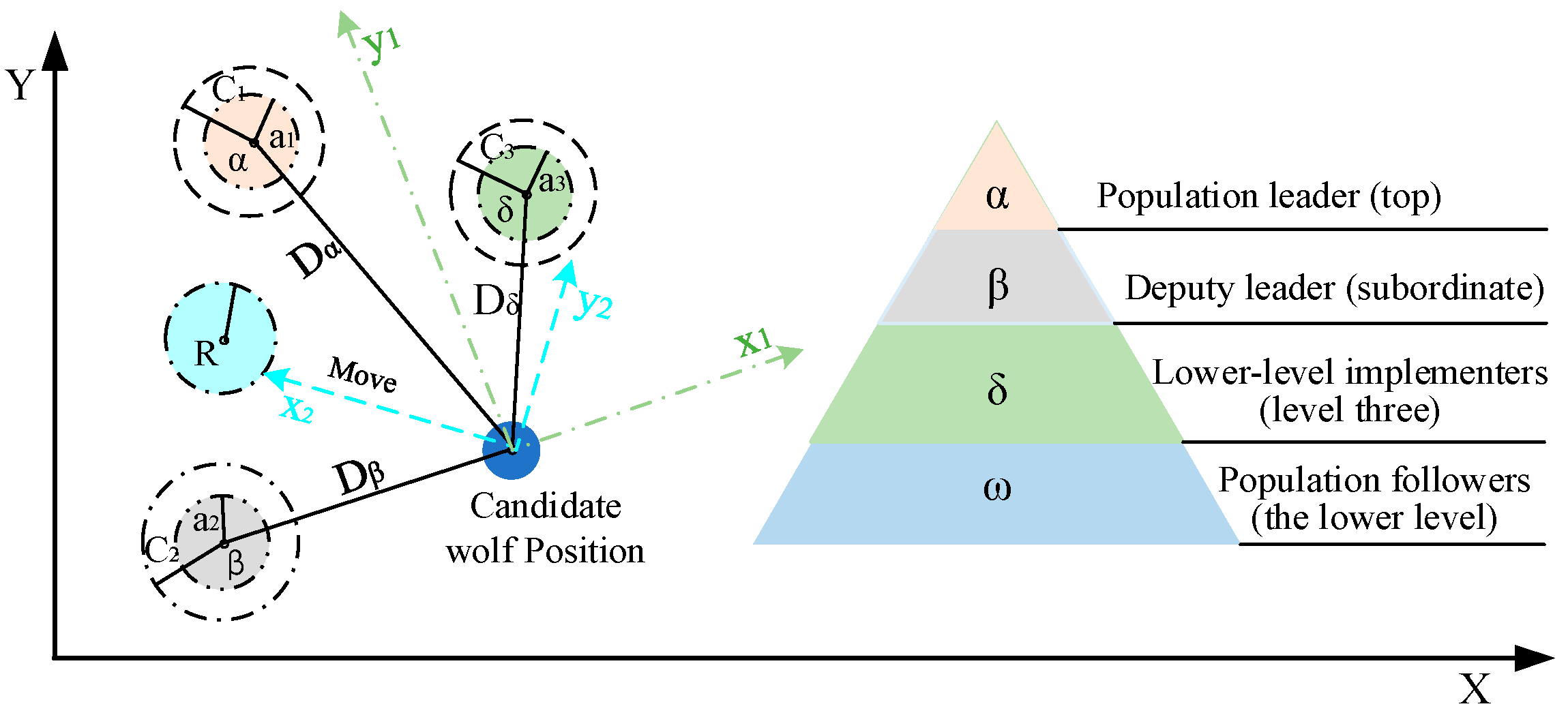
All Gray Wolf Optimizer (GWO) is a population-based optimization algorithm inspired by the hunting behavior and social hierarchy of gray wolves. The algorithm categorizes individuals into four roles: alpha (α), beta (β), delta (δ), and omega (ω), as illustrated in Figure 1, encompassing the entire process of hunting, encircling, and attacking prey. It achieves a balance between global exploration and local exploitation through the iterative adjustment of coefficients A and C, where A decreases over iterations and C is a random number within a defined range.

The process of the Grey Wolf Optimizer (GWO) algorithm is outlined in Algorithm 1, involving key parameters such as population size $N$, dimensionality $\dim$, maximum number of iterations $T_{\max }$, and boundary initialization $[lb,ub]$. During the iterative process, a new position $X_i^{(t)}$ is constructed using the decreasing coefficient $A$ which varies with each iteration, along with random coefficients $s_k$ and $C_k$. After applying boundary constraints to the newly generated position, the three hierarchical roles of gray wolves (α, β, δ) are updated based on their fitness values.

Algorithm 1: GWO Algorithm Workflow

Input: $N$, $T_{\max }$, $\dim$, $[\mathrm{lb},\mathrm{ub}]$

Output: $X^{*}$; $f^{*}$

1 $X_i^{(0)}lb+s_i\odot (ub-lb), i=1,2,\dots ,N // s_i\sim U(0,1)$

2 $f(X_i^{(0)})evaluate\_fitness(X_i^{(0)})$

3 $X_{\alpha }^{(0)}=\arg {\min }_{i}f(X_i^{(0)})$

4 $X_{\beta }^{(0)}=\arg {\min }_{i\ne \alpha }f(X_i^{(0)})$

5 $X_{\delta }^{(0)}=\arg {\min }_{i\ne \alpha ,\beta }f(X_i^{(0)})$

6 $\mathbf{for} t =1 \mathbf{to} T_{\max } \mathbf{do}$

7    $a^{(t)}=2\left(1-t/T_{\max }\right)$

8    $\mathbf{for} i =1 \mathbf{to} N \mathbf{do}$

9      $C_k=2s_k,k=1, 2, 3 // s_k\sim U(0,1)$

10     $D_{\alpha ,i}^{(t)}=|C_1\odot X_{\alpha }^{(t-1)}-X_i^{(t-1)}|$, $D_{\beta ,i}^{(t)}=|C_2\odot X_{\beta }^{(t-1)}-X_i^{(t-1)}|$

11      $D_{\delta ,i}^{(t)}=|C_3\odot X_{\delta }^{(t-1)}-X_i^{(t-1)}|$

12     $A_k=2a^{(t)}{s}_{k+3}-a^{(t)},k=1, 2, 3 // s_{k+3}\sim U(0,1)$

13     $X_1^{(c)}=X_{\alpha }^{(t-1)}-A_1\odot D_{\alpha ,i}^{(t)}$, $X_2^{(c)}=X_{\beta }^{(t-1)}-A_2\odot D_{\beta ,i}^{(t)}$

14     $X_3^{(c)}=X_{\delta }^{(t-1)}-A_3\odot D_{\delta ,i}^{(t)}$

15     $X_i^{(t)}=1/3\left(X_1^{(c)}+X_2^{(c)}+X_3^{(c)}\right)$

16     $\mathbf{for} j =1 \mathbf{to} \dim \mathbf{do}$

17        $\mathbf{if}{ \mathrm{X}}_{i,j}^{(t)}<{\mathrm{lb}}_j \mathbf{then}$

18         $X_{i,j}^{(t)}l{b}_j$

19      end

20      $\mathbf{if}{ \mathrm{X}}_{i,j}^{(t)}>{\mathrm{ub}}_j \mathbf{then}$

21         $X_{i,j}^{(t)}u{b}_j$

22      $\mathbf{end}$

23     $\mathbf{end}$

24   $\mathbf{end}$

25    $f(X_i^{(t)})\mathrm{evaluate}\_\mathrm{fitness}(X_i^{(t)}) X_{\alpha }^{(t)},X_{\beta }^{(t)},X_{\delta }^{(t)}=\arg \mathrm{top}3{\min }_{i}f(X_i^{(t)})$

26  $\mathbf{end}$

27  $\mathbf{return}$ $X^{*}=X_{\alpha }^{(T_{\max })}$, $f^{*}=f\left(X_{\alpha }^{(T_{\max })}\right)$

Initialize the position of each gray wolf individual by setting the population size of the gray wolf group as $N$, and initialize the position $X_i^0$ of the $i$ gray wolf as follows.

$$X_i^0\in {ℝ}^{\dim }=\mathrm{lb}+s_i\odot (ub-lb), i=1,2,3,\dots ,N$$

(1)

In the formula, $i$ represents the index of individuals within the gray wolf population. $lb$ and $ub$ denote the lower and upper bound vectors of the search space, respectively. ${ℝ}^{\dim }$ signifies the d-dimensional real number space. $s_i$ indicates the random vector for the $i$ gray wolf, which is uniformly distributed in the interval [0, 1]. The symbol $\odot$ denotes element-wise multiplication.

By calculating the fitness of each gray wolf in the initial population, the “leadership hierarchy” of the population is determined. This process is used to identify the positions of the top three individuals: the best (α), the second-best (β), and the third-best (δ) wolves.

$$\left\{\begin{array}{l}{X}_{\alpha }^{(0)}=\arg {\min }_{i}f(X_i^{(0)})\hfill \\ X_{\beta }^{(0)}=\arg {\min }_{i\ne \alpha }f(X_i^{(0)})\hfill \\ X_{\delta }^{(0)}=\arg {\min }_{i\ne \alpha ,\beta }f(X_i^{(0)})\hfill \end{array}\right.$$

(2)

In the formula, $X_{\alpha }^{(0)}$, $X_{\beta }^{(0)}$, and $X_{\delta }^{(0)}$ represent the position vectors of α, β, and δ wolves at the initial time $t=0$, respectively. $X_i^{(0)}$ denotes the position vector of the first gray wolf at the initial time. $\arg {\min }_i$ performs traversal over all gray wolves for index $i$. $f(X_i^{(0)})$ represents the fitness value of the $i$ gray wolf. The traversal range for $i\ne \alpha$ excludes gray wolves already selected as α, while the traversal range for $i\ne \alpha ,\beta$ excludes gray wolves already selected as α and β. The fitness function is evaluated to determine the fitness value of each individual’s position. To balance global and local exploration diversity, a dynamic adjustment model is introduced as follows.

$$a^{(t)}=2\left(1-{\displaystyle \frac{t}{T_{\max }}}\right)$$

(3)

In the formula, $t$ denotes the current number of iterations, $a^{(t)}$ represents the control parameter at iteration t, and $T_{\max }$ indicates the maximum number of iterations of the algorithm. The positions of α, β, and δ wolves are utilized to continuously update the positions of the remaining wolves [24] as follows.

$$\left\{\begin{array}{l}{D}_{\alpha ,i}^{(t)}=|C_1\odot X_{\alpha }^{(t-1)}-X_i^{(t-1)}|\hfill \\ D_{\beta ,i}^{(t)}=|C_2\odot X_{\beta }^{(t-1)}-X_i^{(t-1)}|\hfill \\ D_{\delta ,i}^{(t)}=|C_3\odot X_{\delta }^{(t-1)}-X_i^{(t-1)}|\hfill \\ C_k=2r_k,k=1, 2, 3\hfill \end{array}\right.$$

(4)

In the formula, $D_{\alpha ,i}^{(t)}$, $D_{\beta ,i}^{(t)}$, and $D_{\delta ,i}^{(t)}$ represent the distance vectors between the $i$ gray wolf and the α, β, and δ wolves at iteration t, respectively. $X_{\alpha }^{(t-1)}$, $X_{\beta }^{(t-1)}$, and $X_{\delta }^{(t-1)}$ denote the position vectors of the α, β, and δ wolves at iteration t − 1. $X_i^{(t-1)}$ represents the position vector of the $i$ gray wolf at iteration t − 1. The symbol $\odot$ stands for element-wise product, and $|\cdot |$ denotes the absolute value operation. Since $r_k$ represents random numbers in the range [0, 1], $C_k$, together with $C_1$, $C_2$, and $C_3$, represent random coefficient vectors in the range [0, 2]. The candidate location model [25] is calculated as follows.

$$\left\{\begin{array}{l}{X}_1^{(c)}=X_{\alpha }^{(t-1)}-A_1\odot D_{\alpha ,i}^{(t)}\hfill \\ X_2^{(c)}=X_{\beta }^{(t-1)}-A_2\odot D_{\beta ,i}^{(t)}\hfill \\ X_3^{(c)}=X_{\delta }^{(t-1)}-A_3\odot D_{\delta ,i}^{(t)}\hfill \\ A_k=2a^{(t)}{s}_{k+3}-a^{(t)},k=1, 2, 3\hfill \end{array}\right.$$

(5)

In the formula, $X_{\alpha }^{(t-1)}$, $X_{\beta }^{(t-1)}$, $X_{\delta }^{(t-1)}$, $D_{\alpha ,i}^{(t)}$, $D_{\beta ,i}^{(t)}$, $D_{\delta ,i}^{(t)}$, $\odot$, and $|\cdot |$ have the same meanings as in Formula (4) above, and $a^{(t)}$ has the same meaning as in Formula (3) above. $X_1^{(t)}$, $X_2^{(t)}$, and $X_3^{(t)}$ represent the candidate position vectors guided by the leader wolves α, β, and δ, respectively. Since $s_{k+3}$ represents a random number with a value range of [0, 1], $A_k$, $A_1$, $A_2$, and $A_3$ represent the direction control coefficients with a value range of $[-a^{(t)},a^{(t)}]$. By combining the guidance of the leader wolves with random disturbances, the average of the final three candidate positions is used to update the new position $X_i^{(t)}$ of the gray wolf [26,27].

$$X_i^{(t)}={\displaystyle \frac{1}{3}}\left(X_1^{(c)}+X_2^{(c)}+X_3^{(c)}\right)$$

(6)

After completing the position update of the new gray wolf, boundary constraint processing is performed.

$$x_{i,j}^{(t)}=\left\{\begin{array}{l}{\mathrm{lb}}_j \mathrm{if} x_{i,j}^{(t)}{ < \mathrm{lb}}_j\hfill \\ {\mathrm{ub}}_j \mathrm{if} x_{i,j}^{(t)}{ > \mathrm{ub}}_j , \mathrm{j}=1,2,\dots ,\dim \hfill \\ x_{i,j}^{(t)} \mathrm{if} x_{i,j}^{(t)} \mathrm{otherwise}\hfill \end{array}\right.$$

(7)

In the formula, $j$ represents the dimension index, $l{b}_j$ and $u{b}_j$ denote the lower and upper bounds of the $j$ dimension of the search space, respectively, and $x_{i,j}^{(t)}$ represents the $j$ dimensional component of the position of the $i$ gray wolf at iteration t. The best three solutions are reselected by calculating the fitness of the new population.

$$X_{\alpha }^{(t)},X_{\beta }^{(t)},X_{\delta }^{(t)}=\arg \underset{i}{\mathrm{top}3}\min f(X_i^{(t)})$$

(8)

In the formula, $X_{\alpha }^{(0)}$, $X_{\beta }^{(0)}$, and $X_{\delta }^{(0)}$ denote the position vectors of α, β, and δ wolves in generation t, respectively, i denotes the individual index of grey wolves. $\arg \mathrm{top}3\min$ represents the selection of the three individuals with the best fitness values. $X_i^{(t)}$ represents the position vector of the $i$ gray wolf at iteration t, and $f(X_i^{(t)})$ represents the fitness value of the $i$ gray wolf at iteration t. Finally, the global optimal solution is output.

$$\left\{\begin{array}{l}{X}^{*}=X_{\alpha }^{(T_{\max })}\hfill \\ f^{*}=f\left(X_{\alpha }^{(T_{\max })}\right)\hfill \end{array}\right.$$

(9)

In the formula, $X^{*}$ denotes the global optimal solution, $f^{*}$ represents the optimal fitness value, $T_{\max }$ signifies the maximum number of iterations, and $X_{\alpha }^{(T_{\max })}$ indicates the position of the α-wolf at the final iteration.

3. Double-Layer GWOP Fusion Algorithm Design

3.1. GAT Layer Attention Mechanism

GAT (Graph Attention Mechanism) is a neural network built upon graph structures, and its algorithmic flow is outlined in Algorithm 2. By constructing association weights between nodes through adaptive learning, GAT accurately captures the relationships between nodes and their neighbors. It relies on the linear transformation of node features combined with the Softmax normalization function to perform weighted aggregation of neighbor information. Furthermore, GAT enhances the representation of key feature information through multi-head attention concatenation.

Algorithm 2: GAT Attention Mechanism Workflow

Input: $G$, $d_f$, $K$, $d_h$, $E$, $\eta$, $B$, $\lambda$

Output: $GAT \mathsf{\Theta }$

1 $W_k=\mathrm{RandomMatrix}(d_h,d_f)\forall k\in \{1,2,\dots ,K\}$

2 $a_k=\mathrm{RandomVector}(2d_h)\forall k\in \{1,2,\dots ,K\}$

3 $\mathsf{\Theta }=\{W_1,a_1,W_2,a_2,\dots ,W_K,a_K\}$

4 $\mathbf{for} \mathrm{epoch} =1 \mathbf{to} \mathrm{E} \mathbf{do}$

5     $\mathbf{foreach}{ \mathrm{G}}_b\in \mathrm{MiniBatch} (G,B) \mathbf{d}\mathbf{o}$

6      $H_0=\mathrm{ExtractNodeFeatures}(G_b)$

7      $\mathbf{for} k=1 \mathbf{to} K \mathbf{do}$

8      ${H^{\prime }}_k=W_k\cdot H_0$

9      $\mathbf{foreach} (i,j)\in G_b \mathbf{do}$

10      ${h^{\prime }}_{k,k}={H^{\prime }}_k[i]$

11     ${h^{\prime }}_{k,k}={H^{\prime }}_k[j]$

12     $e_{i,j,k}=\mathrm{LeakyReLU}(a_k^T\cdot [{h^{\prime }}_{i,k};{h^{\prime }}_{j,k}])$,

13     ${e^{\prime }}_k[i,j]=e_{i,j,k}$

14      $\mathbf{end}$

15      $a_k=\mathrm{Softmax}(e_k,\dim =1)$

16      ${h^{″}}_{i,k}={\displaystyle {\sum }_{j\in N(i)}{\alpha }_{i,j,k}\cdot {h^{\prime }}_{j,k}}$

17      $z_k[i]=\mathrm{ELU}({h^{″}}_{i,k})$

18     $\mathbf{end}$

19     $Z=\mathrm{Concat}(Z_1,Z_2,\dots ,Z_K)$

20     ${\Gamma }_b=\mathrm{ComputeLoss}(Z,\mathrm{target})$

21    $\Gamma =\Gamma +{\Gamma }_b+\lambda \cdot ||\Theta |{|}_2^2$

22    $\Theta =\Theta -\eta \cdot {\nabla }_{\Theta }\Gamma$

23    $\mathbf{end}$

24  $\mathbf{end}$

25  $\mathbf{return}$ $\Theta$

The weight matrix ${\mathrm{W}}_k\in {ℝ}^{d_h\times d_f}$, attention coefficient vector ${\mathrm{a}}_k\in {ℝ}^{2d_h}$, and parameter vector of each attention head $k\in \{1,2,\dots ,K\}$ [28] are initialized as follows.

$$\left\{\begin{array}{l}{\mathrm{W}}_k{=\mathrm{RandomMatrix}(\mathrm{d}}_h{,\mathrm{d}}_f),\forall k\in \{1,2,\dots ,K\}\hfill \\ {\alpha }_k{=\mathrm{RandomVector}(2\mathrm{d}}_h),\forall k\in \{1,2,\dots ,K\}\hfill \end{array}\right.$$

(10)

In the formula, $ℝ$ represents the real number field, $d_h$ denotes the feature dimension of the node, $d_f$ indicates the initial feature dimension of the node, and ${ℝ}^{d_h\times d_f}$ represents the dimension of the weight matrix ${\mathrm{W}}_k$. K represents the number of attention heads. For each attention head k, the initial feature $H_0$ is linearly transformed using the weight matrix ${\mathrm{W}}_k$.

$${H^{\prime }}_k=W_k\cdot H_0\in {ℝ}^{N\times d_h}$$

(11)

In the formula, $H_0$ represents the initial node feature matrix, $N$ denotes the number of batch nodes, and ${H^{\prime }}_k$ indicates the node feature matrix after transformation. To capture the “UAV-obstacle” obstacle avoidance association [29] and achieve a better trajectory, by combining the attention vector with $\mathrm{LeakyReLU}$ dynamic calculation, the feature correlation coefficient $e_{i,j,k}$ [30,31] after concatenating neighboring node changes is computed as follows:

$$e_{i,j,k}=\mathrm{LeakyReLU}\left(a_k^T\cdot [{h^{\prime }}_{i,k}\oplus {h^{\prime }}_{j,k}]\right)$$

(12)

In the formula, $a_k$ represents the attention vector of the k attention head, and $Leaky\mathrm{Re}LU$ denotes the activation function. ${h^{\prime }}_{i,k}$ represents the feature change in node j under the k attention head, as well as the feature change in its neighbors under the same attention head. $\oplus$ denotes the feature concatenation operation. To address the issue that “different neighbors have different effects on the current node,” for each node i, the neighbor attention coefficient is normalized using the following function $Soft\max$ [32]:

$${\alpha }_{i,j,k}=\mathrm{Softmax}(e_{i,j,k}|j\in \mathbb{N}(i))$$

(13)

In the formula, $\mathbb{N}(i)$ denotes the set of neighbors for node i, and ${\alpha }_{i,j,k}$ represents the normalized attention weight assigned by node i to its j neighbor under the k attention head. By incorporating the characteristics of unmanned aerial vehicles (UAVs) into the “nearest obstacle distance” feature, and subsequently aggregating the flight path features of UAVs, adaptive aggregation of neighboring features can be achieved [33].

$$\left\{\begin{array}{l}{h^{″}}_{i,k}={\displaystyle {\sum }_{j\in \mathbb{N}(i)}{\alpha }_{i,j,k}\cdot {h^{\prime }}_{j,k}}\hfill \\ Z_k[i]=\mathrm{ELU}({h^{″}}_{i,k})\hfill \end{array}\right.$$

(14)

In the formula, ${h^{″}}_{i,k}$ denotes that node i is under the k attention head, aggregating the neighbor features ${\displaystyle {\sum }_{j\in \mathbb{N}(i)}{\alpha }_{i,j,k}\cdot {h^{\prime }}_{j,k}}$, which signifies the weighted summation operation; $Z_k[i]$ represents the output feature of node i under the k attention head, and ELU refers to the exponential linear unit, primarily utilized to break the dependency of linear features.

$$\mathrm{ELU}(x)=\left\{\begin{array}{c}x\hspace{1em} \mathrm{x}\ge 0\\ \alpha (e^x-1) \mathrm{x}<0\end{array}\right.$$

(15)

In the formula, α represents a constant. The complementary modes of different attention heads capture nodes by utilizing multi-attention head concatenation to output the node matrix Z:

$$Z=\mathrm{Concat}\left(Z_1,Z_2,\dots ,Z_K\right)\in {ℝ}^{N\times (K\cdot d_h)}$$

(16)

In the formula, $Z_k$ denotes the output feature matrix of the k attention head, Concat refers to the feature concatenation operation, and $K\cdot d_h$ represents the feature dimension after concatenation. Finally, by quantifying the prediction error of the model, overfitting can be prevented, enabling GAT to progressively learn more characteristic information about dangerous obstacles:

$$\left\{\begin{array}{l}{\Gamma }_b=\mathrm{ComputeLoss}(Z,\mathrm{target}) \hfill \\ \Gamma =\Gamma +{\Gamma }_b+\lambda \cdot ||\Theta |{|}_2^2\hfill \\ \Theta =\Theta -\eta \cdot {\nabla }_{\Theta }\Gamma \hfill \end{array}\right.$$

(17)

In the formula, ${\Gamma }_b$ denotes the predicted loss for the specified batch; Z signifies the features of the model’s output nodes, and target indicates the true value labels of the nodes. $\lambda$ represents the regularization coefficient; $\Theta$ denotes the set of model parameters, $||\Theta |{|}_2^2$ refers to the $L2$ regularization term, and $\Gamma$ represents the total loss. $\eta$ stands for the learning rate, and ${\nabla }_{\Theta }\Gamma$ represents the gradient of the loss function with respect to parameter $\Theta$, which is primarily used to characterize the current changing trend of the loss function with respect to the parameter.

3.2. Group Relative Policy Optimization

The GRPO (Group Relative Policy Optimization) algorithm is illustrated in Figure 2. Its design eliminates the Critic model, thereby overcoming the limitations of large-scale training inherent in traditional reinforcement learning methods. The core idea of GRPO is to derive an estimation benchmark by comparing multiple output results against one another, enabling optimal conclusion inference for value-free networks.

The GRPO algorithm process is outlined in Algorithm 3, starting with the initial strategy ${\pi }_{\theta }$. In the nested loop, a batch $D_b$ is first sampled from the dataset D, and G actions are collected from this batch using strategy ${\pi }_{{\theta }_{old}}$ to compute the action rewards. By constructing the objective function $J_{GRPO}(\theta )$ and integrating it with the dominant function $A_i$, the gradient strategy parameter G is updated.

Algorithm 3: GRPO Algorithm Workflow

Input: ${\pi }_{{\theta }_{init}}$, $r_{\phi }$, $D$, $\epsilon$, $\beta$, $u$

Output: ${\pi }_{\theta }$

1 ${\pi }_{\theta }={\pi }_{{\theta }_{init}}$

2 $\mathbf{for} \mathrm{step} =1 \mathbf{to} I \mathbf{do}$

3    ${\pi }_{\mathrm{ref}}={\pi }_{\theta }$

4    $\mathbf{for} \mathrm{step} =1 \mathbf{to} I \mathbf{do}$

5   $\mathrm{Sample} a \mathrm{batch} D_b \mathrm{from} D$

6    ${\pi }_{{\theta }_{old}}={\pi }_{\theta }$

7    $\mathbf{foreach} q \in D_b \mathbf{do}$

8     $\mathrm{Sample} G \mathrm{oupputs} {\left\{o_i\right\}}_{i=1}^G~{\pi }_{{\theta }_{old}}(o|q)$

9     $\mathbf{for} i =1 \mathbf{to} G \mathbf{do}$

10      $r_i{r}_{\varphi }(o_i,q)$

11     $\mathbf{end}$

12      ${\mathrm{mean}}_r = {\displaystyle \frac{1}{G}}{\displaystyle \sum _{i=1}^G{r}_i}$, ${\mathrm{std}}_r = \sqrt{{\displaystyle \frac{1}{G}}{\displaystyle \sum _{i=1}^G{(r_i-mea{n}_r)}^2}}$

13      $\mathbf{for} i =1 \mathbf{to} G \mathbf{do}$

14      ${\tilde{r}}_i={\displaystyle \frac{r_i-{\mathrm{mean}}_r}{{\mathrm{std}}_r}}$

15      $\mathbf{end}$

16    $\mathbf{end}$

17    $\mathbf{for} \mathrm{GRPO}=1\mathbf{to}u\mathbf{do}$

18      $J_{\mathrm{GRPO}}(\theta )=E_{q~P(Q),{\left\{o_i\right\}}_{i=1}^G~{\pi }_{{\theta }_{\mathrm{old}}}(o|q)}\left[{\displaystyle \frac{1}{G}}{\displaystyle \sum _{i=1}^G\psi }-\beta D_{\mathrm{KL}}({\pi }_{\theta }||{\pi }_{\mathrm{ref}})\right]$

19     $\psi =\min \left({\displaystyle \frac{{\pi }_{\theta }(o_i|q)}{{\pi }_{\mathrm{old}}(o_i|q)}}{A}_i,clip\left({\displaystyle \frac{{\pi }_{\theta }(o_i|q)}{{\pi }_{\mathrm{old}}(o_i|q)}},1-\epsilon ,1+\epsilon \right)A_i\right)$

20      $A_i={\displaystyle \frac{r_i-\mathrm{mean}(\{r_1,r_2,\dots ,r_G\})}{\mathrm{std}(\{r_1,r_2,\dots ,r_G\})}}$

21      $\theta \leftarrow \theta +\eta \cdot {\nabla }_{\theta }J(\theta )$

22      $\mathbf{end}$

23     $\mathbf{end}$

24     $\mathrm{Update} r_{\varphi }u \sin \mathrm{g} a \mathrm{replay} \mathrm{buffer} \mathrm{with} \mathrm{samples} \{(q,o,r_{\varphi }(o,q))\}$

25  $\mathbf{end}$

26  $\mathbf{return}$ ${\pi }_{\theta }$

The GRPO objective function primarily comprises three components: the sampling ratio of old and new policies, the policy clipping objective, and the KL divergence regularization term. In contrast to the classic PPO algorithm, the GRPO algorithm does not require a value network and predominantly employs group sampling to achieve efficient advantage estimation. The continuous update model of the strategy is realized by enhancing the reward-penalty mechanism within the objective function [34] as follows:

$$J_{GRPO}(\theta )=E_{q~P(Q),{\left\{o_i\right\}}_{i=1}^G~{\pi }_{{\theta }_{old}}(o|q)}\left[{\displaystyle \frac{1}{G}}{\displaystyle \sum _{i=1}^G\psi }-\mathfrak{M}\right]$$

(18)

In the above formula, $J_{GRPO}(\theta )$ denotes the objective function value of the GRPO model; E represents the mathematical expectation for sampling from the problem distribution $P(q)$ and the output group generated by the old strategy. $q\sim P(q)$ signifies sampling the input based on the task probability. ${\left\{o_i\right\}}_{i=1}^G\sim {\pi }_{{\theta }_{old}}(o|q)$ indicates generating G candidate outputs from the old strategy q for each sampled ${\pi }_{{\theta }_{old}}$. ${\displaystyle \frac{1}{G}}{\displaystyle \sum \begin{array}{c}G\\ i=1\end{array}}$ refers to averaging the G candidate outputs within each group. $\psi$ and $\mathfrak{M}$ represent the strategy clipping objective and the KL divergence regularization term, respectively [35].

$$\left\{\begin{array}{l}\psi =\min \left(\xi A_i,clip\left(\xi ,1-\epsilon ,1+\epsilon \right)A_i\right)\hfill \\ \mathfrak{M}=\beta D_{KL}({\pi }_{\theta }||{\pi }_{ref})\hfill \end{array}\right.$$

(19)

In the above formula, $\epsilon$ denotes the clipping threshold, and $clip\left(\xi ,1-\epsilon ,1+\epsilon \right)$ signifies the threshold limit of the strategy amplitude. $\beta$ represents the weight of the regularization term, primarily serving to balance strategy improvement and reference constraints. ${\pi }_{ref}$ refers to the reference strategy, and $D_{KL}({\pi }_{\theta }||{\pi }_{ref})$ indicates the KL divergence between strategy ${\pi }_{\theta }$ and the reference strategy ${\pi }_{ref}$. $\xi$ and $A_i$ represent the sampling ratio of the old and new strategies and the estimated intra-group advantage, respectively:

$$\left\{\begin{array}{l}\xi ={\displaystyle \frac{{\pi }_{\theta }(o_i|q)}{{\pi }_{old}(o_i|q)}}\hfill \\ A_i={\displaystyle \frac{r_i-mean(\{r_1,r_2,\dots ,r_G\})}{std(\{r_1,r_2,\dots ,r_G\})}}\hfill \end{array}\right.$$

(20)

In the above formula, ${\pi }_{\theta }(o_i|q)$ denotes the probability of the current strategy generating $o_i$, and ${\pi }_{old}(o_i|q)$ signifies the probability of the old strategy generating $o_i$ prior to the update. When $\xi >1$, it indicates that the new strategy is more likely to generate $o_i$; when $\xi <1$, it suggests that the new strategy reduces the generation probability of $o_i$. $r_i$ represents the original reward for the i output, $mean(\{r_1,r_2,\dots ,r_G\})$ denotes the average of all rewards within the group, and $std(\{r_1,r_2,\dots ,r_G\})$ signifies the standard deviation of all rewards within the group. When $A_i>0$, it implies that the output performs better than the group average; when $A_i<0$, it implies that the output performs worse than the group average.

3.3. Double-Layer GWOP Algorithm Design

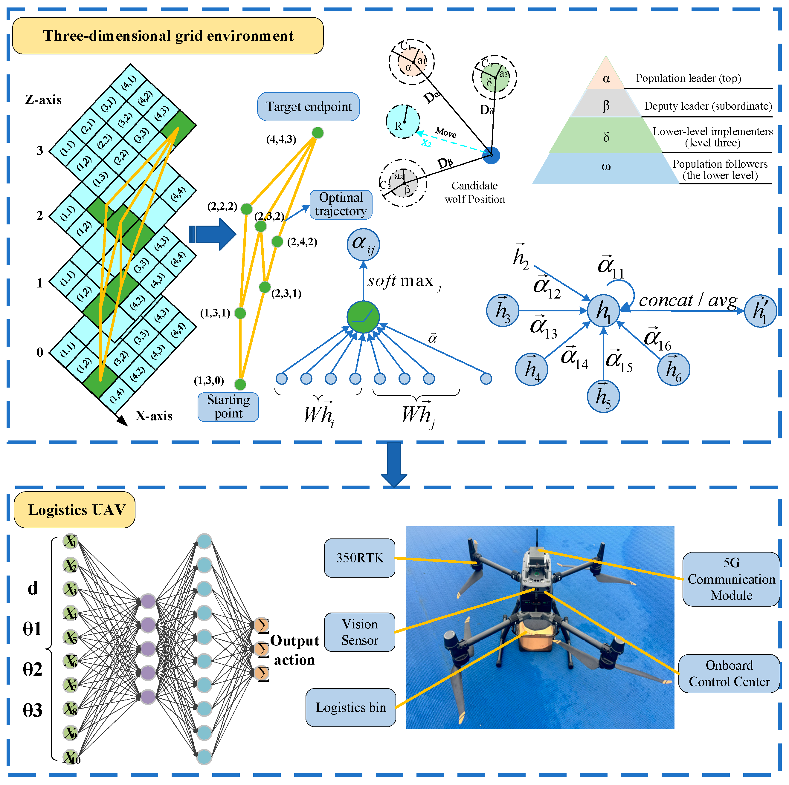
The two-layer fusion GWOP algorithm integrates the combination process of GWO and GRPO, with the introduction of the GAT attention mechanism, as illustrated in the overall fusion framework shown in Figure 3. Through the three-dimensional raster coding environment depicted in the upper left of the figure, the representation of digital spatial grid information is completed [36]. By meticulously recording the performance of each trajectory algorithm in 3D route planning, fast search and accurate evaluation of the optimal route planning algorithm are achieved. The top right corner of the figure presents the fundamental framework of the Gray Wolf Optimization (GWO). Building upon this, the GAT attention mechanism in the bottom right corner and the GRPO algorithm are fused to form a comprehensive integration process of “GWO group search + GRPO strategy optimization + GAT graph structure perception.” Finally, the output results are applied to the attitude control of the UAV in the bottom right corner, providing an effective solution for real-time path planning of logistics UAVs in unknown environments.

The process of the GWOP fusion algorithm is outlined in Algorithm 4. Firstly, the GRPO algorithm is integrated into the GWO fitness calculation as $J_c=J_{GRPO}({\theta }_c)$. On this basis, the GAT attention mechanism is incorporated to establish the association of key feature information, serving as the fitness constraint term $J_{GRPO}({\theta }_i)=f_{task}({\theta }_i)+\lambda \cdot GAT(G,{\theta }_i)$ for the GWO algorithm. The solution for the complete optimal strategy is achieved via bidirectional collaborative feedback between GAT attention weights and GWO strategies.

Algorithm 4: Double—Layer GWOP fusion Algorithm Workflow

Input: $N$, $T_{\max }$, $\dim$, $[\mathrm{lb},\mathrm{ub}]$, $\mathrm{GRPO}$, $\epsilon$     $\beta$, $G$, $d_h$, $d_h$, $K$, $E$, $\eta$, $B$, $\lambda$

Output: ${\theta }^{*}$, $J_{\mathrm{GRPO}}^{\ast }$, $\mathrm{GAT} \Theta$, $\mathrm{G}\mathrm{W}\mathrm{O}\mathrm{P}$

1 ${\theta }_i=\mathrm{lb}+s_i\odot (\mathrm{ub}-\mathrm{lb}),s_i\sim U{(0,1)}^{\dim }$

2 $\mathbf{for} i=1 \mathbf{to} N \mathbf{do}$

3   $J_i=J_{\mathrm{GR}\mathrm{PO}}({\theta }_i)$

4   $f_i=J_i$

5 $\mathbf{end}$

6 ${\theta }_{\alpha }=\arg {\min }_i{f}_i$

7 ${\theta }_{\beta }=\arg {\min }_{i\ne \alpha }{f}_i$

8 ${\theta }_{\delta }=\arg {\min }_{i\ne \alpha ,\beta }{f}_i$

9 $\mathbf{for} \mathrm{t}=1 \mathbf{to} T_{\max } \mathbf{do}$

10     $a=2(1-t/T_{\max })$

11     $\mathbf{for} i =1 \mathbf{to} N \mathbf{do}$

12     $\mathbf{for} k=1\mathbf{to} 3 \mathbf{do}$

13      $r_k=\mathrm{Random}(0,1)$

14      $C_k=2r_k,k=1, 2, 3 // r_k\sim U(0,1)$

15      $D_{\alpha ,i}=|C_1\odot {\theta }_{\alpha }-{\theta }_i|$

16      $D_{\beta ,i}=|C_2\odot {\theta }_{\beta }-{\theta }_i|$

17      $D_{\delta ,i}=|C_3\odot {\theta }_{\delta }-{\theta }_i|$

18     $\mathbf{end}$

19     $\mathbf{for} k=1 \mathbf{to} 3 \mathbf{do}$

20      $s_{k+1}=\mathrm{Random}(0,1)$

21      $A_k=2a{s}_{k+3}-a,k=1, 2, 3 // s_{k+3}\sim U(0,1)$

22      ${\theta }_k^{(c)}={\theta }_{\{\alpha ,\beta ,\delta \}[k]}-A_k\odot D_{\{\alpha ,\beta ,\delta \}[k],i}$

23  $\mathbf{end}$

24  ${\theta }_c=1/3\left({\theta }_1^{(c)}+{\theta }_2^{(c)}+{\theta }_3^{(c)}\right)$

25  $\mathbf{for}j =1\mathbf{to} \dim \mathbf{do}$

26   $\mathbf{if}{\theta }_{c,j}<{\mathrm{lb}}_j \mathbf{then}$

27    ${\theta }_{c,j}={\mathrm{lb}}_j$

28   $\mathbf{end}$

29   $\mathbf{if} {\theta }_{c,j}>{\mathrm{ub}}_j \mathbf{then}$

30     ${\theta }_{c,j}\leftarrow u{b}_j$

31   $\mathbf{end}$

32  $\mathbf{end}$

33  $J_c=J_{\mathrm{GRPO}}({\theta }_c)$

34  $f_c=J_c$

35  $\mathbf{if} f_c<f_i \mathbf{then}$

36    ${\theta }_i={\theta }_c$

37    $f_j=f_c, J_j=J_c$

38  $\mathbf{end}$

39 $\mathbf{end}$

40 ${\theta }_{\alpha },{\theta }_{\beta },{\theta }_{\delta }=\arg \mathrm{top}3{\min }_i{f}_i$

41 $\mathbf{end}$

42 ${\theta }^{*}={\theta }_{\alpha }$

43 $J_{GRPO}^{\ast }=-f({\theta }_{\alpha })$

44 $\mathbf{if} k=1 \mathbf{to} K \mathbf{do}$

45 $W_k=\mathrm{RandomMatrix}(d_h,d_f)$

46 $a_k=\mathrm{RandomVector}(2d_h)$

47 $\mathbf{end}$

48 $\mathsf{\Theta }=\{W_1,a_1,W_2,a_2,\dots ,W_K,a_K\}$

49 $\mathbf{for} \mathrm{epoch}=1 \mathbf{to} E \mathbf{do}$

50 $\mathbf{foreach} G_b\in \mathrm{MiniBatch}(G,B)\mathbf{do}$

51   $H_0=\mathrm{ExtractNodeFeatures}(G_b)$

52   $\mathbf{for} k=1\mathbf{to}K \mathbf{do}$

53   ${H^{\prime }}_k=W_k\cdot H_0$

54   $\mathbf{foreach} (i,j)\in G_b \mathbf{do}$

55     ${h^{\prime }}_{k,k}={H^{\prime }}_k[i]$

56    ${h^{\prime }}_{k,k}={H^{\prime }}_k[j]$

57    $e_{i,j,k}=\mathrm{LeakyReLU}(a_k^T\cdot [{h^{\prime }}_{i,k};{h^{\prime }}_{j,k}])$,

58    ${e^{\prime }}_k[i,j]\leftarrow e_{i,j,k}$

59   $\mathbf{end}$

60   $a_k=\mathrm{Softmax}(e_k,\dim =1)$

61   ${h^{″}}_{i,k}={\displaystyle {\sum }_{j\in N(i)}{\alpha }_{i,j,k}\cdot {h^{\prime }}_{j,k}}$

62   $z_k[i]=\mathrm{ELU}({h^{″}}_{i,k})$

63   $\mathbf{end}$

64   $Z=\mathrm{Concat}(Z_1,Z_2,\dots ,Z_K)$

65   ${\Gamma }_b=\mathrm{ComputeLoss}(Z,\mathrm{target})$

66   $\Gamma =\Gamma +{\Gamma }_b+\lambda \cdot ||\Theta |{|}_2^2$

67   $\Theta =\Theta -\eta \cdot {\nabla }_{\Theta }\Gamma$

68  $\mathbf{end}$

69  $\mathbf{end}$

70  $\mathbf{return}$ ${\theta }^{*},J_{GRPO}^{*} , \Theta$

The GWO “Wolf Pack” corresponds to a set of candidate strategies for logistics drones, which comprises multiple ${\theta }_i$ strategy parameters. Under any selected parameter of Strategy ${\theta }_i$, dynamic trajectory planning and goods distribution are executed by the logistics unmanned aerial vehicle. The trajectory performance under Strategy ${\theta }_i$ is evaluated using the GRPO algorithm, and ultimately the optimal “α Wolf” guided population evolution is achieved. By integrating the two-tier architecture of GWO and GRPO, the GWOP algorithm realizes a high-quality global/local search strategy. The initialization of the GWOP model [37] is as follows:

$$\left\{\begin{array}{l}{\theta }_i\in {ℝ}^{\dim }=\mathrm{lb}+s_i\otimes (\mathrm{ub}-\mathrm{lb}) , s_i\sim U{(0,1)}^{\dim }\hfill \\ W_k\sim N(0,{\sigma }^2), a_k\sim N(0,{\sigma }^2), k=1,2,\dots ,K\hfill \end{array}\right.$$

(21)

In the formula, $\theta$ denotes the parameter vector of the reinforcement learning strategy, $ℝ$ represents the real number field, and dim signifies the dimension of the strategy parameters. ${\theta }_i$ represents the strategy parameters of the i individual in the population. $lb$ denotes the lower bound of the parameters, $ub$ denotes the upper bound of the parameters, $s_i$ represents the random vector where each element follows a uniform distribution in (0,1). $\otimes$ signifies element-wise multiplication. $W_k$ represents the weight matrix of the k attention head, $a_k$ represents the attention coefficient vector of the k attention head, k denotes the index of the attention head, and K represents the total number of attention heads. The reward value model in the fitness evaluation of GRPO [38] is as follows:

$$\left\{\begin{array}{l}{\tilde{r}}_i={\displaystyle \frac{r_i-{\mathrm{mean}}_r}{{\mathrm{std}}_r}}\hfill \\ {\mathrm{mean}}_r={\displaystyle \frac{1}{G}}{\displaystyle {\sum }_{i=1}^G{r}_i}\hfill \\ {\mathrm{std}}_r=\sqrt{{\displaystyle \frac{1}{G}}{\displaystyle {\sum }_{i=1}^G{(r_i-{\mathrm{mean}}_r)}^2}}\hfill \end{array}\right.$$

(22)

In the formula, $r_i$ denotes the original reward of the i sampling, and ${\tilde{r}}_i$ denotes the standardized reward of the i sampling. G represents the number of samplings for the same type of action, $mea{n}_r$ represents the arithmetic mean of the rewards for G samplings, and ${\mathrm{std}}_r$ represents the standard deviation of the rewards for G samplings. The fitness $J({\theta }_i)$ of the i gray wolf individual in the modified GRPO objective function is [39,40,41]:

$$\left\{\begin{array}{l}{J}_{\mathrm{GRPO}}({\theta }_i)=f_{\mathrm{task}}({\theta }_i)+\lambda \cdot \mathrm{GAT}(G,{\theta }_i)\hfill \\ f_{\mathrm{task}}=E_{q~P(Q),o~{\pi }_{{\theta }_{\mathrm{old}}}(o|q)}\left[{\displaystyle \frac{1}{G}}{\displaystyle \sum _{i=1}^G\psi }-\beta D_{\mathrm{KL}}({\pi }_{{\theta }_i}||{\pi }_{{\theta }_{\mathrm{old}}})\right]\hfill \\ \psi =\min \left({\displaystyle \frac{{\pi }_{{\theta }_i}(o|q)}{{\pi }_{{\theta }_{\mathrm{old}}}(o|q)}}\cdot {\tilde{r}}_i,clip\left({\displaystyle \frac{{\pi }_{{\theta }_i}(o|q)}{{\pi }_{{\theta }_{\mathrm{old}}}(o|q)}},1-\epsilon ,1+\epsilon \right)\cdot {\tilde{r}}_i\right)\hfill \end{array}\right.$$

(23)

In the formula, $f_{task}({\theta }_i)$ denotes the task objective function, $\psi$ denotes the objective term, $\lambda$ denotes the balance coefficient, $GAT(G,{\theta }_i)$ denotes the graph structure constraint term, and G denotes the graph structure data. E represents the expectation operation, q represents the environmental state, and $P(Q)$ represents the state distribution; o represents the actions performed by the agent in state q, and ${\pi }_{{\theta }_{\mathrm{old}}}(o|q)$ represents the action distribution of the old policy. G denotes the number of action samples in the same state, and ${\displaystyle \sum _{i=1}^G\psi }$ denotes the sum of $\psi$ for G action samples. $\beta$ represents the penalty coefficient of KL divergence, and $D_{\mathrm{KL}}({\pi }_{\theta }||{\pi }_{\mathrm{ref}})$ represents KL divergence. ${\theta }_i$ denotes the parameters of the current candidate strategy, and ${\theta }_{old}$ denotes the parameters of the old strategy; ${\displaystyle \frac{{\pi }_{{\theta }_i}(o|q)}{{\pi }_{{\theta }_{\mathrm{old}}}(o|q)}}$ represents the probability difference in the output action o between the new and old strategies in state q, $\epsilon$ represents the clipping coefficient, and $\mathrm{clip}\left({\displaystyle \frac{{\pi }_{{\theta }_i}(o|q)}{{\pi }_{{\theta }_{\mathrm{old}}}(o|q)}},1-\epsilon ,1+\epsilon \right)$ indicates clipping the input value to the interval $[1-\epsilon ,1+\epsilon ]$. The model for converting the maximization objective of GRPO into the minimization objective of GWO is:

$$f({\theta }_i)=-J_{\mathrm{GRPO}}(\theta )$$

(24)

In the formula, $J_{\mathrm{GRPO}}(\theta )$ denotes the performance evaluation value of GRPO for strategy ${\pi }_{{\theta }_i}$, and $f({\theta }_i)$ denotes the fitness function value of the i individual in GWO. Coefficients of the GWO update mechanism [42,43]:

$$\left\{\begin{array}{l}{a}^{(t)}=2\left(1-t/T_{\max }\right)\hfill \\ C_k=2r_k, r_k\sim U(0,1),k=1, 2, 3 \hfill \\ A_k=2a^{(t)}{s}_{k2}-a^{(t)},s_{k2}\sim U(0,1),k=1, 2, 3 \hfill \end{array}\right.$$

(25)

In the formula, t denotes the current number of iterations, and $T_{\max }$ denotes the maximum number of iterations. $r_k$ and $r_{k2}$ represent uniformly distributed random numbers within the range (0, 1). $C_k$ represents the bounding coefficient, and $A_k$ represents the direction coefficient [44].

$$\left\{\begin{array}{l}{h^{\prime }}_i=W_k\cdot h_i,\forall i\in \nu \hfill \\ e_{i,j}=\mathrm{LeakyReLU}(a_k^T\cdot [{h^{\prime }}_i;{h^{\prime }}_j]),\forall (i,j)\in \epsilon \hfill \\ {\alpha }_{i,j}={\displaystyle \frac{\exp (e_{i,j})}{{\displaystyle {{\sum }_{k\in \mathbb{N}(i)}}^{\exp (e_{i,k})}}}} \hfill \\ {h^{″}}_i={\displaystyle {\sum }_{j\in \mathbb{N}(i)}{\alpha }_{i,j}\cdot {h^{\prime }}_j}\hfill \end{array}\right.$$

(26)

In the formula, $h_i$ denotes the original feature vector of node i, $W_k$ denotes the weight matrix of the k attention map, ${h^{\prime }}_i$ denotes the updated feature vector of node i, and $\nu$ represents the node set of the graph. $e_{i,j}$ represents the original attention coefficient between nodes i and j, $a_k^T\cdot [{h^{\prime }}_i;{h^{\prime }}_j]$ represents the inner product operation between nodes, $[{h^{\prime }}_i;{h^{\prime }}_j]$ denotes the feature concatenation operation, and $\epsilon$ represents the edge set of the graph. ${\alpha }_{i,j}$ represents the normalized attention weight of node i to neighbor j, $\exp (e_{i,j})$ denotes the exponential transformation of the original attention coefficient, ${\displaystyle {{\sum }_{k\in \mathbb{N}(i)}}^{\exp (e_{i,k})}}$ represents the sum of the exponential attention coefficients for all neighbors of the node i, and $\mathbb{N}(i)$ denotes the neighbor set of node i. ${h^{″}}_i$ represents the new feature vector after node i aggregates the features of its neighbors, and ${\displaystyle {\sum }_{j\in \mathbb{N}(i)}{\alpha }_{i,j}\cdot {h^{\prime }}_j}$ denotes the weighted summation operation. $C_k$ represents the containment coefficient, which measures the distance from the Wolf pack and is used for candidate strategy updates [45]:

$$\left\{\begin{array}{l}{D}_{\alpha }=|C_1\otimes {\theta }_{\alpha }-{\theta }_i|\hfill \\ D_{\beta }=|C_2\otimes {\theta }_{\beta }-{\theta }_i|\hfill \\ D_{\delta }=|C_3\otimes {\theta }_{\delta }-{\theta }_i|\hfill \\ {\theta }_1^{(c)}={\theta }_{\alpha }-A_1\otimes D_{\alpha }\hfill \\ {\theta }_2^{(c)}={\theta }_{\beta }-A_2\otimes D_{\beta }\hfill \\ {\theta }_3^{(c)}={\theta }_{\delta }-A_3\otimes D_{\delta }\hfill \\ {\theta }_c=({\theta }_1^{(c)}+{\theta }_2^{(c)}+{\theta }_3^{(c)})/3\hfill \end{array}\right.$$

(27)

In the formula, ${\theta }_{\alpha }$, ${\theta }_{\beta }$, ${\theta }_{\delta }$, and ${\theta }_i$ respectively denote the current optimal strategy, suboptimal strategy, third optimal strategy, and the parameter vector of the current individual. $\otimes$ represents element-wise multiplication. $D_{\alpha }$, $D_{\beta }$, and $D_{\delta }$ respectively denote the parameter difference vectors of the α, β, and δ wolf. ${\theta }_1^{(c)}$, ${\theta }_2^{(c)}$, and ${\theta }_3^{(c)}$ respectively denote the candidate parameter vectors of the α, β, and δ wolf. ${\theta }_c$ denotes the final candidate strategy that integrates the three leader-guided strategies. The values of $A_1$, $A_2$, and $A_3$ are dynamically adjusted by the output of GAT [46]:

$$A_k=2a\cdot (1+\gamma \cdot {\mathrm{GAT}}_{\mathrm{attention}}(i,j))-a$$

(28)

In the formula, $A_k$ denotes the control coefficient for the position update of the gray wolf, a denotes the basic control parameter of GWOP, $\gamma$ denotes the scaling factor, ${\mathrm{GAT}}_{\mathrm{attention}}(i,j)$ represents the attention weight function calculated by the GAT model for node, where i is the current node and j is a neighboring node. The greedy update and convergence model [47] is as follows:

$$\left\{\begin{array}{l}\Theta =\Theta -\eta \cdot {\nabla }_{\Theta }[L_{\mathrm{task}}+\lambda \cdot L_{\mathrm{GWOP}}]\hfill \\ {\theta }^{*}={\theta }_i^{(\mathrm{new})} \mathrm{if} J({\theta }_i^{(\mathrm{new})})>J({\theta }_i)\hfill \end{array}\right.$$

(29)

In the formula, $\Theta$ denotes the set of learning parameters of GAT, $\eta$ denotes the learning rate, and ${\nabla }_{\Theta }$ denotes the gradient of the loss function with respect to $\Theta$. $L_{task}$ represents the task-specific loss, $\lambda$ represents the balance coefficient, and $L_{\mathrm{GWOP}}$ represents the GWOP guiding loss. ${\theta }_i^{(new)}$ denotes the new position of the i gray wolf individual, and $J({\theta }_i^{(\mathrm{new})})$ denotes the fitness function corresponding to the new position of the i gray wolf individual. ${\theta }_i$ represents the current position of the i gray wolf individual, and $J({\theta }_i)$ represents the fitness function corresponding to the current position of the i gray wolf individual.

3.4. B-Spline Trajectory Curve

In the application of B-spline trajectory curves to the delivery routes of logistics drones, given the node vector $\mathrm{U}=\{u_0,u_1,\dots ,u_m\}$, the $i$ $p$ degree basis function $N_{i,p}(u)$ is defined as follows:

$$\left\{\begin{array}{l}{N}_{i,0}(u)=\left\{\begin{array}{l}1{ \mathrm{u}}_i\le u\le u_{i+1}\hfill \\ 0 \mathrm{otherwise}\hfill \end{array}\right.\hfill \\ N_{i,p}(u)={\displaystyle \frac{u-u_i}{u_{i+p}-u_i}}\cdot N_{i,p-1}(u)+{\displaystyle \frac{u_{i+p-1}-u}{u_{i+p+1}-u_{i+1}}}\cdot N_{i+1,p-1}(u)\hfill \end{array}\right.$$

(30)

In the formula, $u_i$ represents the continuous changing values of a non-decreasing sequence of node vectors, and $N_{i,p}(u)$ indicates the $i$$p$ degree B-spline basis function, where $i$ is the index of the basis function and p is the degree of the basis function. For $n+1$ control vertices $P_0,P_0,\dots ,P_0\in {ℝ}^d$, where $d$ is the dimension. The weighted sum of the control vertices of the B-spline curve:

$$C(u)={\displaystyle \sum _{i=0}^n{N}_{i,p}(u)\cdot P_{i}u}\in [u_p,u_{m-p}]$$

(31)

In the above formula, $P_i$ represents the control vertices, $C(u)$ is the B-spline curve function, $m$ is the total number of nodes; $u$ is the parameter variable and serves as the input for the B-spline curve. The minimum smooth model of the B-spline curve is as follows:

$$J={\displaystyle {\int }_{u_0}^{u_n}\left({\omega }_1||\ddot{C}(u)|{|}^2+{\omega }_2||C(u)-Q(u)|{|}^2\right)}du$$

(32)

In the above formula, $J$ represents the objective of the trajectory curve, ${\omega }_1$ and ${\omega }_2$ are the weight coefficients of the curve; $C(u)$ optimizes the B-spline curve, and $\ddot{C}(u)$ is the second derivative of the B-spline curve $C(u)$ with respect to the parameter $u$; $Q(u)$ is the parametric curve, $||C(u)-Q(u)|{|}^2$ is the square of the $L_2$ norm of the difference between the curves $C(u)$ and $Q(u)$, ${\omega }_2||C(u)-Q(u)|{|}^2$ is the penalty for the deviation of the curve from the ideal trajectory $Q(u)$, and ${\omega }_1||\ddot{C}(u)|{|}^2$ is the penalty for the “non-smoothness” of the curve.

4. Experiment and Evaluation

4.1. Experimental Scenario

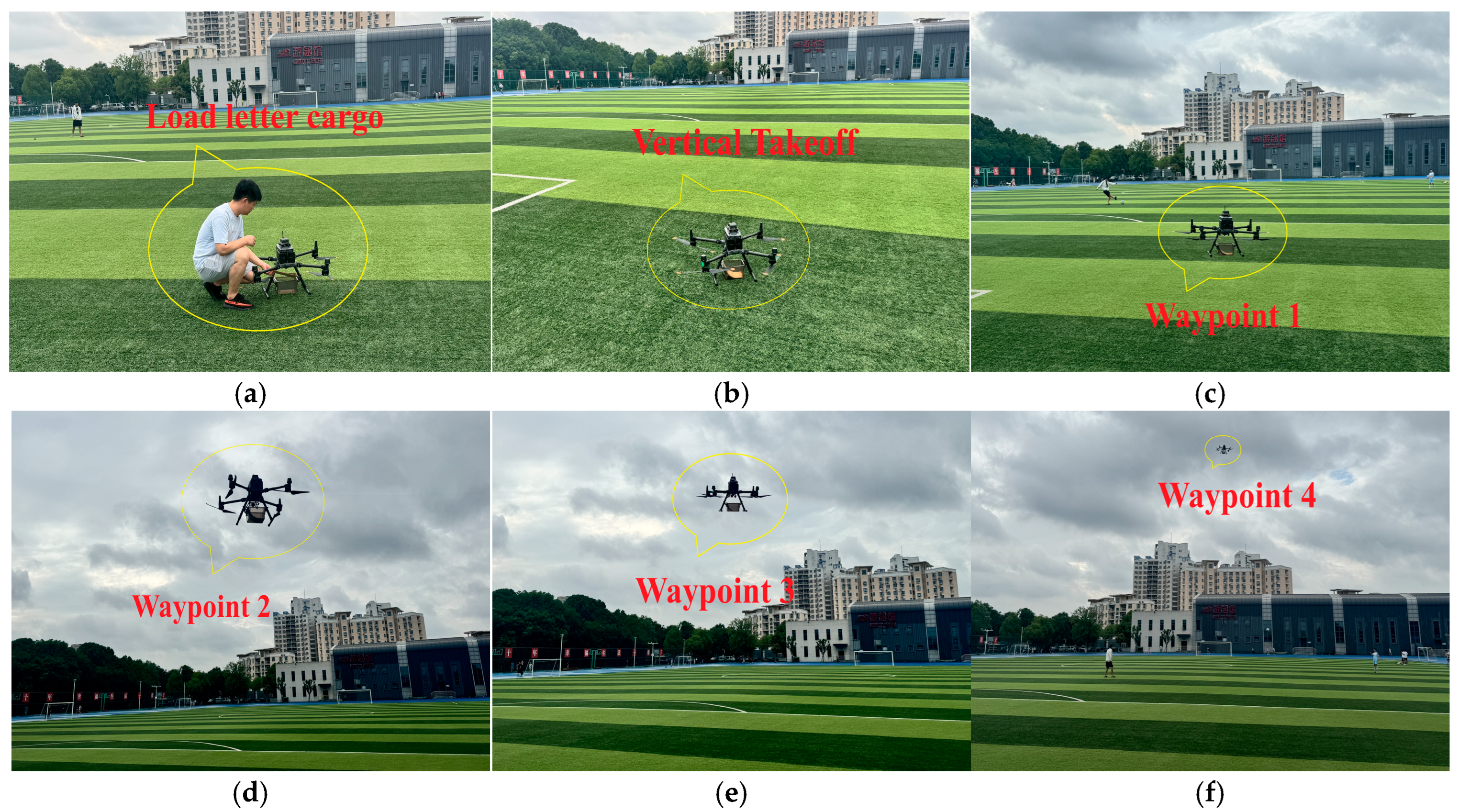
In order to verify the effectiveness of the double-layer GWOP algorithm, which integrates GWO and GRPO, in dynamic route planning for logistics UAVs, the entire flight experiment process of the logistics UAV from “loading—taking off—route planning” is recorded, as shown in Figure 4. Specifically, Figure 4a illustrates the process of loading envelope goods into the UAV logistics box; Figure 4b shows the vertical takeoff of the logistics UAV; and Figure 4c–f depict the various stages of the logistics UAV’s distribution route planning and flight process.

4.2. Experimental Results Analysis

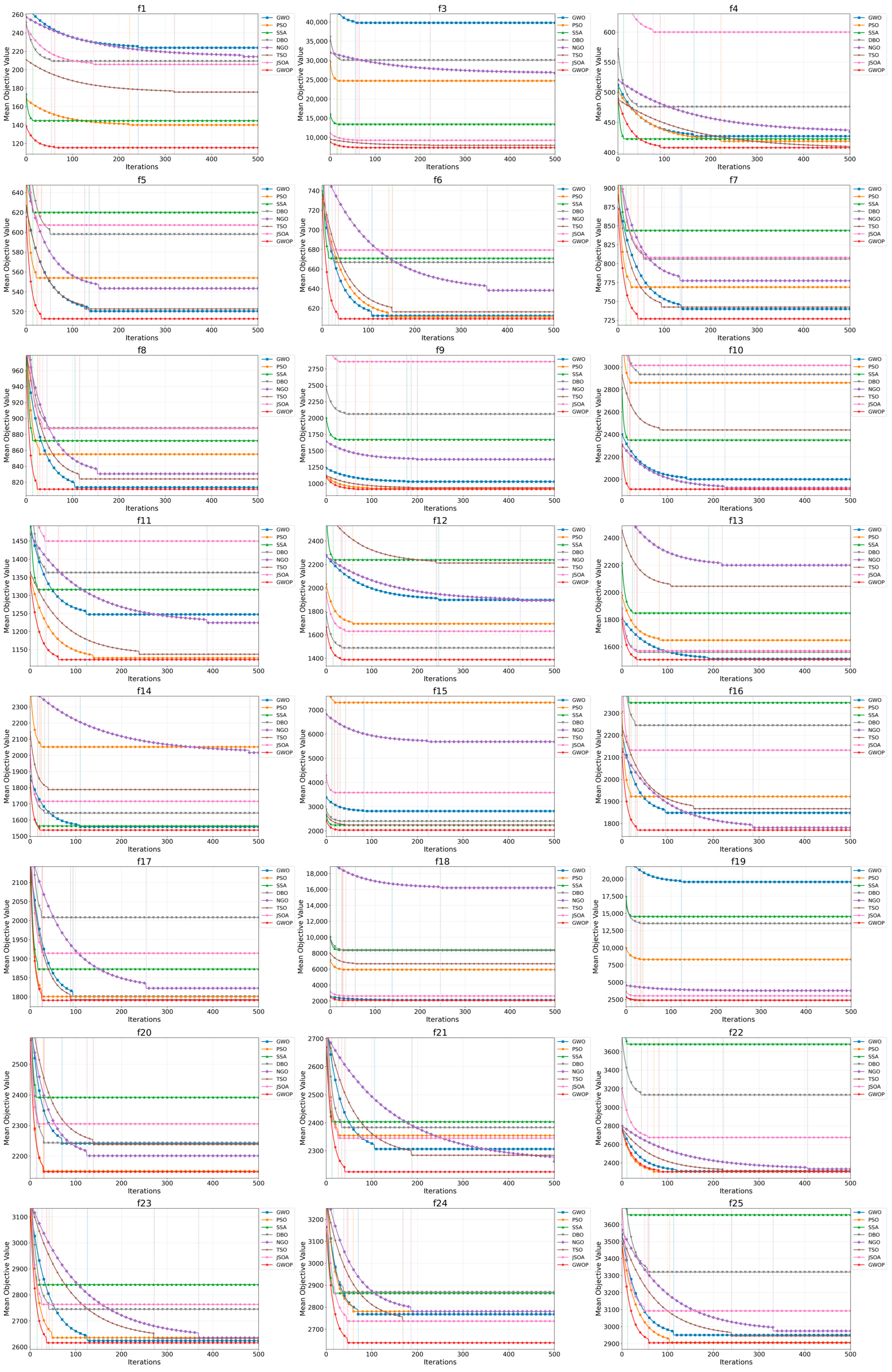
The CEC2017 test functions are listed in

Table 1. CEC2017 test functions.

Function	Function Description	Search Range	Optimum
F1	Shifted and Rotated Bent Cigar	[−100,100]	100
F3	Shifted and Rotated Sum of Power	[−100,100]	300
F4	Shifted and Rotated Rosenbrock	[−100,100]	400
F5	Shifted and Rotated Rastrigin	[−100,100]	500
F6	Shifted and Rotated Schaffer F6	[−100,100]	600
F7	Shifted and Rotated Schwefel	[−100,100]	700
F8	Shifted and Rotated Ackley	[−100,100]	800
F9	Shifted and Rotated Weierstrass	[−100,100]	900
F10	Shifted and Rotated Griewank	[−100,100]	1000
F11	Hybrid Function 1 (N = 3)	[−100,100]	1100
F12	Hybrid Function 2 (N = 3)	[−100,100]	1200
F13	Hybrid Function 3 (N = 3)	[−100,100]	1300
F14	Hybrid Function 4 (N = 4)	[−100,100]	1400
F15	Hybrid Function 5 (N = 4)	[−100,100]	1500
F16	Hybrid Function 6 (N = 4)	[−100,100]	1600
F17	Hybrid Function 6 (N = 5)	[−100,100]	1700
F18	Hybrid Function 6 (N = 5)	[−100,100]	1800
F19	Hybrid Function 6 (N = 5)	[−100,100]	1900
F20	Hybrid Function 6 (N = 6)	[−100,100]	2000
F21	Composition Function 1 (N = 3)	[−100,100]	2100
F22	Composition Function 2 (N = 3)	[−100,100]	2200
F23	Composition Function 3 (N = 4)	[−100,100]	2300
F24	Composition Function 4 (N = 4)	[−100,100]	2400
F25	Composition Function 5 (N = 5)	[−100,100]	2500

. Among these, F1 to F10 are basic transformation functions, primarily used to evaluate convergence performance on unimodal/multimodal and complex curved landscapes through shifting and rotation operations. F11 to F20 represent hybrid functions, mainly designed to assess the algorithm’s ability to collaboratively optimize multiple sub-problems. F21 to F25 are also hybrid functions, specifically intended to test robustness and global search capabilities in highly complex environments, thereby evaluating the comprehensive performance of multiple sub-function superposition and local distortion.

4.3. CEC2017 Test

4.3.1. CEC2017 Test Data

The results of the improved GWOP algorithm and seven other algorithms, namely GWO, PSO, SSA, DBO, NGO, TSO, and JSOA, on the CEC2017 test function data are shown in

Table 2. Data obtained from different algorithms in the basic function.

Function	Algorithm	Min	Mean	Std
F1	GWO	199.6942	223.8952	14.0158
	PSO	111.7409	140.0931	15.8392
	SSA	123.3391	144.8780	12.8837
	DBO	194.1273	209.2599	10.3549
	NGO	200.8044	214.2256	9.7497
	TSO	160.3911	175.7389	10.4338
	JSOA	180.1937	205.7861	14.6241
	GWOP	104.6724	115.3897	8.8722
F3	GWO	28,358.3631	39,774.9904	5710.244
	PSO	17,644.3925	24,685.2489	3353.1221
	SSA	9697.0204	13,455.8940	1889.9365
	DBO	26,192.2466	30,052.3033	1520.5187
	NGO	21,007.2925	26,682.8705	2166.6123
	TSO	7212.8277	7944.1156	370.1362
	JSOA	8603.3870	9232.7826	317.5621
	GWOP	7190.4553	7309.2385	51.8563
F4	GWO	407.4124	426.9561	12.0619
	PSO	401.2658	418.5848	9.0139
	SSA	411.9919	422.6454	10.1980
	DBO	403.9496	475.7415	36.4312
	NGO	400.5129	433.9783	16.7253
	TSO	402.6160	407.0193	3.8720
	JSOA	436.7995	600.0487	87.7498
	GWOP	401.7645	412.8103	8.9721
F5	GWO	504.0811	520.5336	10.8477
	PSO	539.5564	554.0134	10.1109
	SSA	604.9819	620.1995	10.3872
	DBO	582.0188	597.9400	10.6522
	NGO	523.8859	543.3910	12.0463
	TSO	511.9445	522.7534	8.9001
	JSOA	586.9167	607.2735	12.3935
	GWOP	502.0501	512.8086	8.8846
F6	GWO	603.2949	614.3527	8.9760
	PSO	570.2043	610.9744	21.5719
	SSA	658.0606	671.1013	12.0831
	DBO	655.4169	666.7742	9.0800
	NGO	622.6914	638.2184	10.5012
	TSO	601.6734	616.3090	10.1769
	JSOA	659.5449	679.3991	15.8114
	GWOP	602.9636	613.2150	8.7333
F7	GWO	722.4713	739.9215	11.2307
	PSO	751.9333	768.8368	9.7279
	SSA	813.2591	844.1527	21.7951
	DBO	715.9411	805.9927	47.1721
	NGO	752.5464	777.3352	14.2703
	TSO	725.7858	742.4425	10.9262
	JSOA	782.1305	808.2137	14.8347
	GWOP	712.1128	726.9038	8.6603
F8	GWO	804.9292	815.5636	8.8472
	PSO	839.4395	855.1465	9.0143
	SSA	861.4109	872.1668	8.8838
	DBO	867.7398	887.9043	12.3146
	NGO	817.9014	830.4514	7.0711
	TSO	804.9764	824.0656	11.1803
	JSOA	876.4252	887.4550	8.9674
	GWOP	801.4056	812.1789	8.8778
F9	GWO	922.5302	1029.0626	55.9017
	PSO	904.4682	927.0224	13.3106
	SSA	1373.6403	1672.4681	174.6425
	DBO	1443.3348	2058.6789	320.7845
	NGO	1138.4852	1368.5626	138.8741
	TSO	904.5056	935.6467	17.3205
	JSOA	2375.6038	2860.6900	254.9510
	GWOP	902.6817	913.4026	8.8735
F10	GWO	1700.5368	2000.1873	173.2051
	PSO	2563.7048	2860.3803	148.5062
	SSA	2263.0570	2350.6769	51.9615
	DBO	2617.2892	2932.8825	157.9622
	NGO	1739.3814	1923.4420	92.3015
	TSO	1838.0149	2439.8799	316.2278
	JSOA	2835.7767	3015.1094	89.9226
	GWOP	1629.6746	1911.6185	165.8312
F11	GWO	1198.3934	1247.3438	26.9258
	PSO	1111.6025	1126.6918	10.3422
	SSA	1171.3402	1316.1543	81.9152
	DBO	1265.7318	1362.6032	51.9624
	NGO	1126.2361	1224.1619	49.4709
	TSO	1110.6622	1137.0669	15.8114
	JSOA	1209.2471	1449.5850	134.5850
	GWOP	1111.0965	1121.9514	6.7082
F12	GWO	1653.6827	1897.9735	134.1633
	PSO	1385.5648	1694.3517	173.2042
	SSA	2226.2853	2241.0972	10.2396
	DBO	1408.542	1486.5067	43.3029
	NGO	1564.1293	1892.4710	187.0829
	TSO	1794.4268	2213.1708	235.4435
	JSOA	1483.4669	1630.2579	81.9152
	GWOP	1269.0917	1387.2982	67.0822
F13	GWO	1311.1547	1511.6939	100.5186
	PSO	1402.8567	1648.5917	141.4214
	SSA	1654.1679	1849.0739	97.7102
	DBO	1481.5184	1559.6546	43.3011
	NGO	1839.6218	2200.0185	216.3331
	TSO	1977.8453	2045.5321	34.5742
	JSOA	1419.5982	1571.2147	81.9163
	GWOP	1378.7931	1505.1852	70.7107
F14	GWO	1506.7327	1557.7897	28.8675
	PSO	1935.4622	2052.0645	67.0820
	SSA	1308.0316	1563.4021	158.1139
	DBO	1598.8812	1641.9349	25.0031
	NGO	1532.8810	2016.7747	269.2582
	TSO	1519.2942	1787.8413	133.7116
	JSOA	1707.7270	1715.2129	7.8747
	GWOP	1427.1532	1537.1033	55.4259
F15	GWO	2815.5633	2818.8157	1.8708
	PSO	7033.3291	7304.1382	152.0690
	SSA	2239.2530	2246.0180	7.8427
	DBO	2043.6193	2397.3519	205.1346
	NGO	4341.3267	5684.5163	787.4008
	TSO	2106.1466	2246.8089	81.9155
	JSOA	17,002.2270	3581.0996	6928.3242
	GWOP	1973.4003	2032.3893	30.3302
F16	GWO	1624.9880	1848.3706	134.1641
	PSO	1630.8093	1922.1510	165.8312
	SSA	2178.0912	2348.3049	85.3872
	DBO	2031.4753	2244.4391	122.4745
	NGO	1682.1597	1780.9209	49.8843
	TSO	1703.3987	1866.8732	90.1388
	JSOA	1903.2532	2132.3633	134.1642
	GWOP	1618.7213	1769.8372	86.6025
F17	GWO	1740.8918	1801.0265	34.0147
	PSO	1769.0717	1800.7769	19.3649
	SSA	1835.9871	1872.9507	21.7945
	DBO	1879.3856	2007.8020	67.0822
	NGO	1782.3045	1822.4122	23.5442
	TSO	1709.8100	1792.8947	47.1699
	JSOA	1847.8339	1914.2622	37.4157
	GWOP	1765.7882	1790.7650	14.3178
F18	GWO	1920.9610	2121.5875	100.5620
	PSO	4116.8128	5937.1160	1019.8039
	SSA	7174.8955	8420.5290	670.8204
	DBO	7665.1584	8325.8646	370.1364
	NGO	13,392.1282	16,201.4987	1670.8204
	TSO	5928.6741	6672.3475	433.0127
	JSOA	2463.5349	2627.6745	91.2871
	GWOP	1790.3838	2084.8504	173.2052
F19	GWO	12,769.9149	19,578.0563	3741.6574
	PSO	7446.3107	8309.6088	471.6991
	SSA	13,697.6576	14,568.8387	519.6152
	DBO	11,887.5391	13,513.9625	912.8709
	NGO	3321.7081	3785.2513	269.2585
	TSO	2334.3152	2404.0387	37.4166
	JSOA	2618.7474	3027.0182	235.4435
	GWOP	2319.6048	2379.6982	35.3553
F20	GWO	2179.5893	2241.2514	31.6189
	PSO	2046.7955	2150.6669	52.4150
	SSA	2315.9651	2392.3386	43.3013
	DBO	2200.9078	2242.8261	23.5443
	NGO	2147.9662	2200.7338	27.3186
	TSO	2003.4239	2237.6677	136.0147
	JSOA	2290.1059	2305.2064	10.3444
	GWOP	2107.1872	2148.2014	21.6919
F21	GWO	2216.6432	2306.1456	51.9616
	PSO	2340.0154	2354.5055	10.1239
	SSA	2334.1681	2403.8723	35.5621
	DBO	2368.0681	2382.4550	10.0878
	NGO	2204.8040	2261.4396	34.0147
	TSO	2202.4812	2283.9535	45.0185
	JSOA	2262.9841	2344.8427	41.5376
	GWOP	2211.5305	2224.5515	9.6109
F22	GWO	2205.5170	2309.9892	52.7125
	PSO	2201.6532	2305.2766	52.2921
	SSA	3498.0365	3681.4250	101.9804
	DBO	2689.1098	3133.1716	254.9511
	NGO	2305.1063	2333.6546	16.5831
	TSO	2104.1656	2313.4109	122.4746
	JSOA	2371.1417	2674.1010	187.0829
	GWOP	2263.8219	2302.7221	22.3607
F23	GWO	2611.5189	2623.6803	9.3153
	PSO	2614.4655	2635.3773	12.6224
	SSA	2768.6285	2839.4329	42.7200
	DBO	2702.4604	2744.1736	24.0416
	NGO	2615.2458	2634.8083	12.0830
	TSO	2606.3662	2633.2287	15.1789
	JSOA	2713.6315	2763.0923	28.8676
	GWOP	2508.5386	2615.6636	57.0088
F24	GWO	2753.8516	2767.9796	9.9951
	PSO	2749.1593	2780.9635	18.0278
	SSA	2762.8885	2864.3542	51.2213
	DBO	2823.2695	2868.5801	23.7332
	NGO	2756.1069	2780.8886	14.2665
	TSO	2621.0201	2736.4937	58.1682
	JSOA	2608.5651	2736.5884	64.3996
	GWOP	2518.3326	2637.9874	60.2421
F25	GWO	2914.1375	2950.8556	21.7947
	PSO	2892.0841	2907.3512	8.8921
	SSA	3457.2638	3657.8078	100.5210
	DBO	3148.4886	3319.8685	96.0469
	NGO	2912.7585	2974.3931	31.6181
	TSO	2901.1772	2944.9415	22.9964
	JSOA	2945.8707	3092.0851	87.7496
	GWOP	2862.4215	2904.9506	22.4100

. The results of the improved GWOP algorithm and seven other algorithms, including GWO, PSO, SSA, DBO, NGO, TSO, and JSOA, on the CEC2017 test function data are shown in Table 2. The obtained data results include the minimum value Min, the mean value Mean, and the standard deviation Std. The obtained data results include the minimum value Min, the average value Mean, and the standard deviation Std.

4.3.2. CEC2017 Test Results

The results of the improved GWOP algorithm and seven other algorithms GWO, PSO, SSA, DBO, NGO, TSO, and JSOA on the CEC2017 test functions are presented in Figure 5. Based on the convergence curves of the unimodal, multimodal, and composite functions from F1 to F10, it can be observed that the improved two-layer fused GWOP algorithm achieves better convergence performance and lower fitness values compared to the original GWO algorithm. Moreover, the GWOP algorithm consistently obtains the lowest fitness values among all the compared algorithms, including PSO, SSA, DBO, NGO, TSO, and JSOA. Furthermore, GWOP demonstrates superior performance in terms of fitness accuracy for the mixed functions from F11 to F20 and for the complex functions from F21 to F25.

4.4. Experimental Procedure

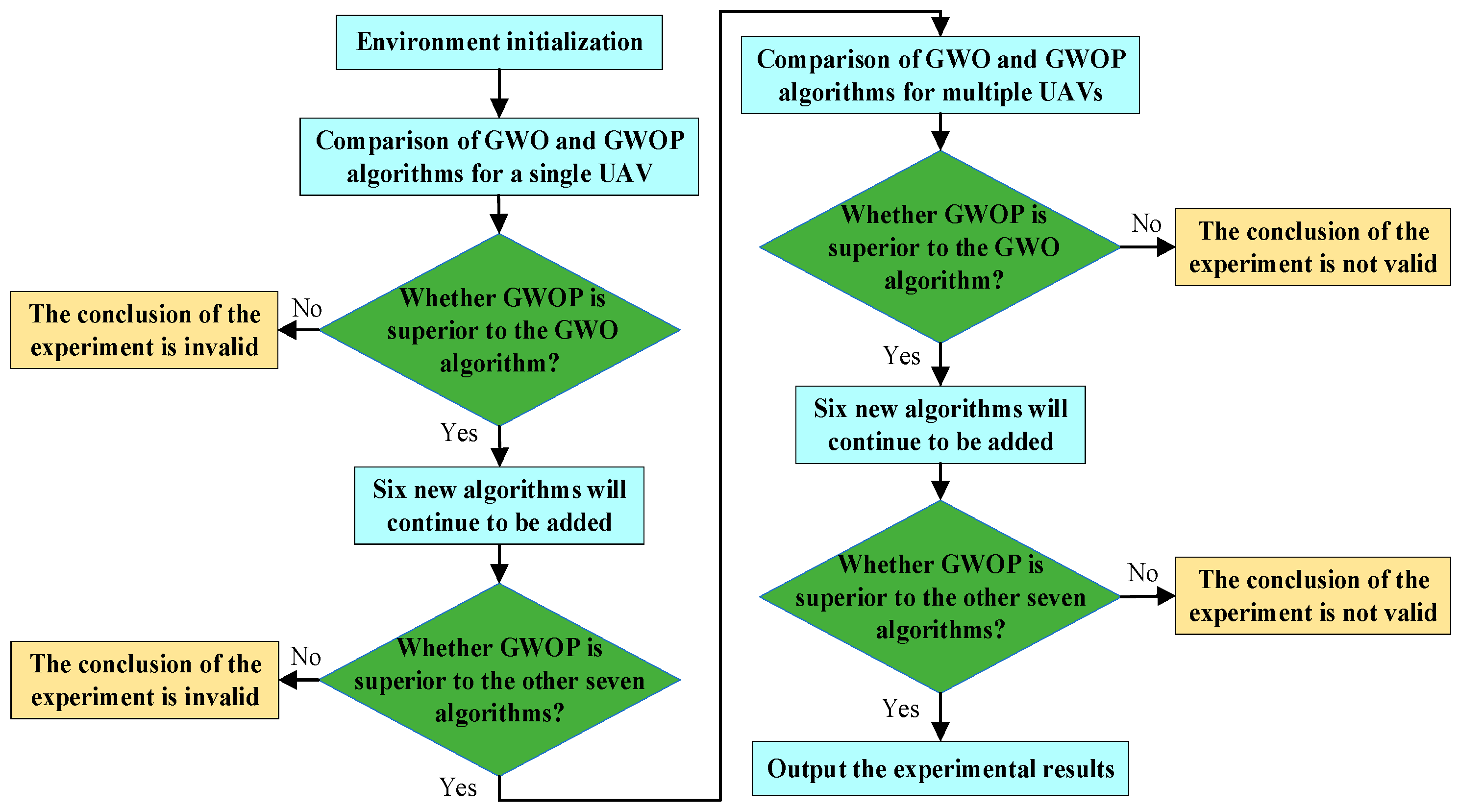
The path planning of logistics UAV involves four experiments, as shown in Figure 6. Experiment 1: The improved double-layer fusion GWOP algorithm is compared with the classical GWO algorithm under a single UAV scenario. Experiment 2: Building upon Experiment 1, six classical 3D trajectory planning algorithms (GWO, PSO, SSA, DBO, NGO, TSO, and JSOA) are introduced for comparison with the improved two-layer fusion GWOP algorithm to determine whether GWOP outperforms these seven algorithms. Experiment 3: The single UAV scenario from Experiment 1 is extended to multiple UAVs to compare the GWOP and GWO algorithms. Experiment 4: The single UAV scenario from Experiment 2 is similarly extended to multiple UAVs to conduct comparative experiments between GWOP and the other seven path planning algorithms.

5. UAV Trajectory Planning Model Design

5.1. Design of UAV Flight Environment

A target model is constructed by integrating the three key factors: shortest trajectory distance [48], smoothness, and minimum collision risk:

$$f={\lambda }_1{\displaystyle {\sum }_{i=1}^{n-1}||P_i-P_{i+1}||}+{\lambda }_2{\displaystyle {\sum }_{i=2}^{n-1}{\theta }_i^2}+{\lambda }_3{\displaystyle {\sum }_{i=1}^n}{\displaystyle {\sum }_{o\in O}\frac{1}{d(P_i,o)+\epsilon }}$$

(33)

In this formula, ${\lambda }_1$, ${\lambda }_2$, and ${\lambda }_3$ denote the weight coefficients corresponding to trajectory length, smoothness, and collision risk, respectively. Based on the specific requirements of trajectory planning for delivery tasks, this study sets the values of ${\lambda }_1=0.6$, ${\lambda }_2=0.2$, and ${\lambda }_3=0.2$.

Logistics unmanned aerial vehicle minimum trajectory distance model:

$$\min f_1={\displaystyle {\sum }_{i=1}^{n-1}||P_i-P_{i+1}||}$$

(34)

In the formula, $P_i$ represents the three-dimensional coordinates of the $i$ waypoint of the unmanned aerial vehicle’s trajectory planning, and $||P_i-P_{i+1}||$ represents the Euclidean distance between two points, which is $\sqrt{{(x_{i+1}-x_i)}^2+{(y_{i+1}-y_i)}^2+{(z_{i+1}-z_i)}^2}$. In the formula, $n$ indicates the total number of waypoints along the trajectory.

The maximum smoothness model of logistics drones:

$$\max f_2={\displaystyle {\sum }_{i=2}^{n-1}{\theta }_i^2}$$

(35)

In the formula, ${\theta }_i$ represents the turning angle at the $i$ waypoint of the drone’s flight path. Then, the angle ${\theta }_i$ between the two vectors needs to satisfy $\cos {\theta }_i={\displaystyle \frac{{\overrightarrow{v}}_i\cdot {\overrightarrow{v}}_{i+1}}{||{\overrightarrow{v}}_i||\cdot ||{\overrightarrow{v}}_{i+1}||}}$, where ${\overrightarrow{v}}_i=P_i-P_{i-1}$ and ${\overrightarrow{v}}_{i+1}=P_{i+1}-P_i$.

Minimum collision risk model for logistics drones in flight among obstacles:

$$\min f_3={\displaystyle {\sum }_{i=1}^n}{\displaystyle {\sum }_{o\in O}\frac{1}{d(P_i,o)+\epsilon }}$$

(36)

In the formula, ${\displaystyle {\sum }_{o\in O}}$ represents the summation over all obstacles, $o$ represents the index of a single obstacle, $O$ represents the set of all obstacles; ${\displaystyle \frac{1}{d(P_i,o)+\epsilon }}$ represents the collision risk between a single planning point and a single obstacle, $d(P_i,o)$ represents the shortest distance from the trajectory point $P_i$ to the obstacle o, and $\epsilon$ represents a very small positive number.

5.2. Construct UAV Flight Constraint Model

5.2.1. Load Constraint

The payload capacity of an unmanned aerial vehicle (UAV) in delivery operations is determined by the difference between its maximum takeoff weight and its empty weight. To account for the payload limitations inherent in logistics UAVs used for cargo transportation, a payload constraint model is formulated:

$$W_{load}\le G_{\max }-W_{empty}$$

(37)

In the formula, $W_{load}$ represents the payload, $G_{\max }$ represents the maximum takeoff weight, $W_{empty}$ represents the empty weight of the drone, and $G_{\max }-W_{empty}$ represents the upper limit of the maximum payload of the drone.

5.2.2. Turning Radius Constraint

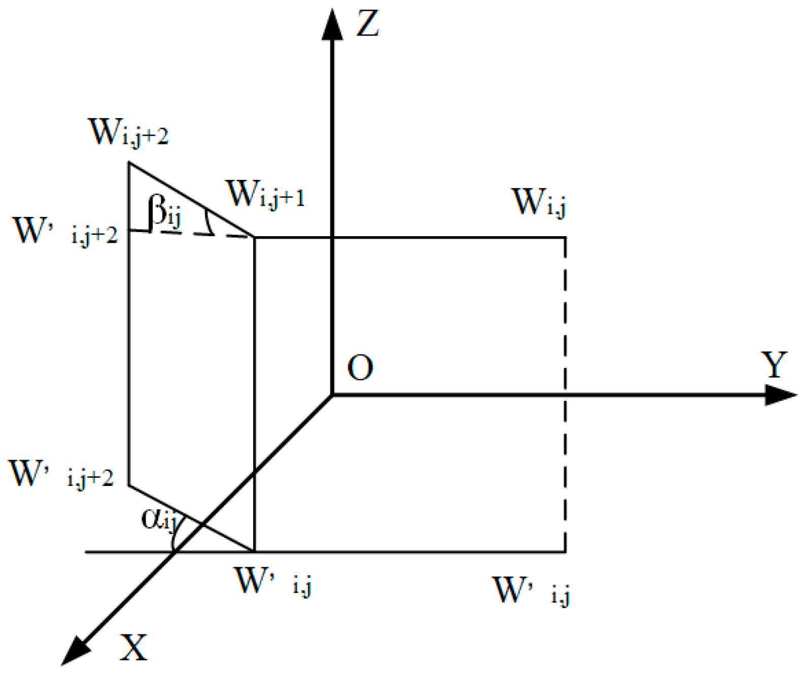
In logistics unmanned aerial vehicle UAV delivery transportation, the turning angle constraints during flight include both vertical and horizontal limitations, as illustrated in Figure 7. Let trajectory point $W_{ij}=(x_{ij},y_{ij},z_{ij})$ represent the $j$ point along the $i$ flight path, where $\overrightarrow{W_{i,j}{W}_{i,j+1}}$ and $\overrightarrow{W_{i,j+1}{W}_{i,j+2}}$ denote two consecutive trajectory segments during flight, and $\overrightarrow{{W^{\prime }}_{i,j}{W^{\prime }}_{i,j+1}}$ and $\overrightarrow{{W^{\prime }}_{i,j+1}{W^{\prime }}_{i,j+2}}$ are the projections of the corresponding flight trajectory onto the horizontal coordinate axis $XOY$.

Reasonable corner constraints significantly contribute to the generation of optimal flight path trajectories. When integrated with the aforementioned flight trajectory construction model:

$$\left\{\begin{array}{l}\overrightarrow{{W^{\prime }}_{i,j}{W^{\prime }}_{i,j+1}}= b\times (\overrightarrow{W_{i,j}{W}_{i,j+1}}\times b)\hfill \\ {\alpha }_{ij}=\arctan \left({\displaystyle \frac{\overrightarrow{{W^{\prime }}_{ij}{W^{\prime }}_{i,j+1}}\times \overrightarrow{{W^{\prime }}_{ij+1}{W^{\prime }}_{i,j+2}}}{\overrightarrow{{W^{\prime }}_{ij}{W^{\prime }}_{i,j+1}}\cdot \overrightarrow{{W^{\prime }}_{ij+1}{W^{\prime }}_{ij+2}}}}\right)\hfill \\ {\beta }_{ij}=\arctan \left({\displaystyle \frac{z_{i,j+1}-z_{i,j}}{\overrightarrow{{W^{\prime }}_{ij}{W^{\prime }}_{i,j+1}}}}\right)\hfill \end{array}\right.$$

(38)

In this formula, ${\alpha }_{ij}$ denotes the horizontal turning angle, ${\beta }_{ij}$ denotes the vertical turning angle, and $b$ represents the unit vector corresponding to the positive direction of each coordinate axis.

5.2.3. Flight Posture Constraint

If the rotation matrix of the logistics unmanned aerial vehicle is set as $R=\left[\begin{array}{ccc}{r}_{11}& r_{12}& r_{13}\\ r_{21}& r_{22}& r_{23}\\ r_{31}& r_{32}& r_{33}\end{array}\right]$, then the corresponding constraints of each attitude angle are as follows:

$$\left\{\begin{array}{l}\theta =\arcsin (-r_{31})\hspace{1em}\hspace{1em}-{\displaystyle \frac{\pi }{6}}\le \theta \le {\displaystyle \frac{\pi }{6}}\hfill \\ \varphi =\arctan 2(r_{32},r_{33})\hspace{1em}-{\displaystyle \frac{\pi }{4}}\le \varphi \le {\displaystyle \frac{\pi }{4}}\hfill \\ \psi =\arctan 2(r_{21},r_{11})\hspace{1em}-\pi \le \psi \le \pi \hfill \end{array}\right.$$

(39)

In this formula, $\theta$ denotes the pitch angle, $\varphi$ denotes the roll angle, and $\psi$ denotes the yaw angle. The corresponding quaternion is represented by $q=(q_0,q_1,q_2,q_3)$, where $q_0$ is the real part. Based on this representation, $\theta =\arcsin (-2(q_1{q}_3-q_0{q}_2))$, $\varphi =\arctan 2(2(q_0{q}_1+q_2{q}_3),q_0^2-q_1^2-q_2^2+q_3^2)$, and $\psi =\arctan 2(2(q_1{q}_2+q_0{q}_3),q_0^2+q_1^2-q_2^2-q_3^2)$ are calculated.

5.2.4. Flight Altitude Constraint

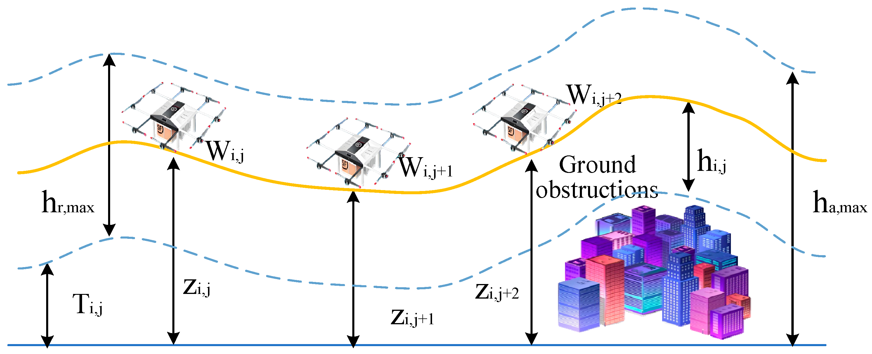
The flight height constraints for the unmanned aerial vehicle UAV are illustrated in Figure 8. The flight altitude of the logistics UAV must comply with the maximum allowable height limit. Specifically, $T_{i,j}$ denotes the terrain elevation at the $j$ waypoint along the $i$ route, ${\mathrm{z}}_{i,j}$ represents the UAV’s flight altitude relative to sea level at that waypoint, $h_{r,\max }$ is the maximum relative flight height, and $h_{a,\max }$ is the maximum absolute flight height.

The flight altitude of the unmanned aerial vehicle must satisfy the following constraint model:

$$H_{i,j}=\left\{\begin{array}{l}\varsigma (h_{a,\max }-T_{i,j}) \mathrm{if} (z_{i,j}-T_{i,j})>h_{a,\max }\hfill \\ z_{i,j}\hspace{1em}\hspace{1em}\hspace{1em}\hspace{1em} \mathrm{else} T_{i,j}<(z_{i,j}-T_{i,j})<h_{a,\max }\hfill \\ \varsigma (h_{ij}+T_{i,j})\hspace{1em} \mathrm{else} (z_{i,j}-T_{i,j})<0\hfill \end{array}\right.$$

(40)

In this formula, $W_{i,j+1}$, $W_{i,j+2}$, $W_{i,j+3}$ and $W_{i,j+4}$ denote the weights corresponding to the $j$, $j+1$, $j+2$, $j+3$, and $j+4$ track points along the $i$ flight route, respectively. $\varsigma$ represents the altitude coefficient, which has a value range of (0, 1), while $H_{i,j}$ denotes the optimized actual flight altitude when reaching the $j$ track point on the $i$ flight route.

5.2.5. Flight Speed Constraint

During the unmanned aerial vehicle (UAV) delivery process, the speed constraint is expressed as:

$$v\le \sqrt{{\displaystyle \frac{T_{\max }^2-G^2}{k_d}}}$$

(41)

In this formula, $v$ denotes the horizontal flight speed, $G$ represents the total load during flight, $k_d$ is the aerodynamic drag coefficient during flight, and $T_{\max }$ denotes the maximum total thrust limit of the unmanned aerial vehicle.

5.3. Simulation Example and Results Analysis

5.3.1. Comparing Single UAV Path Planning Experiments

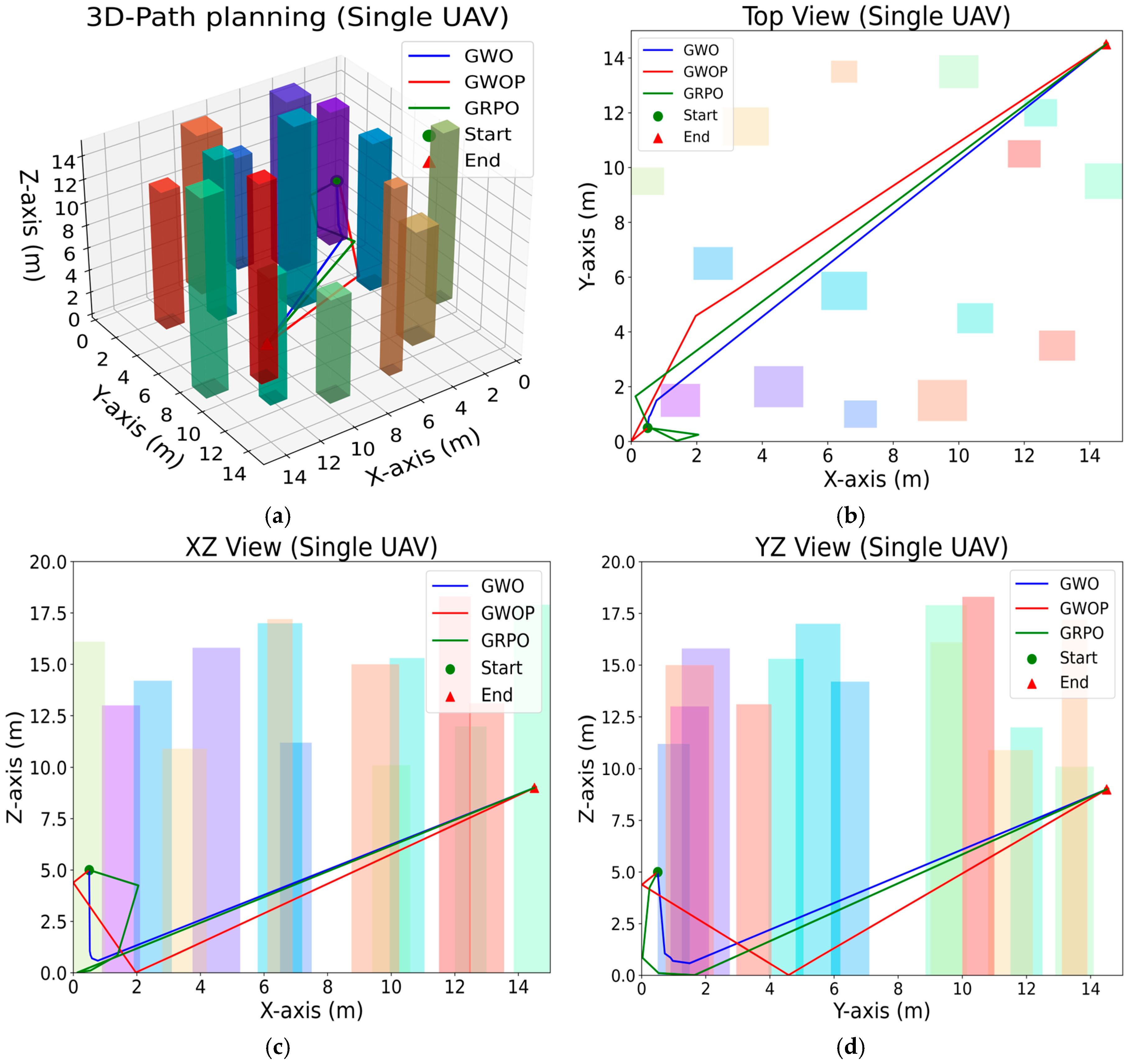
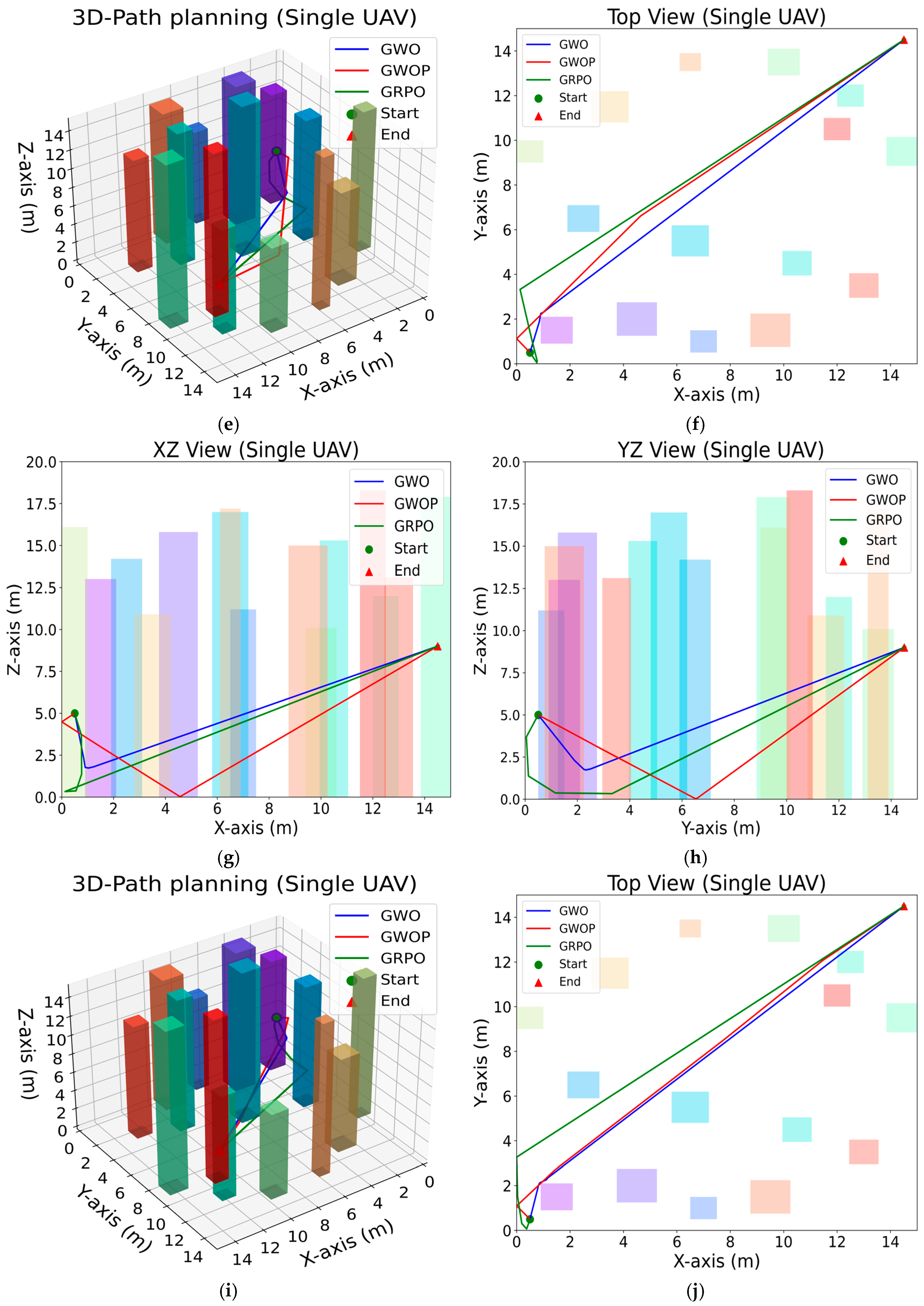
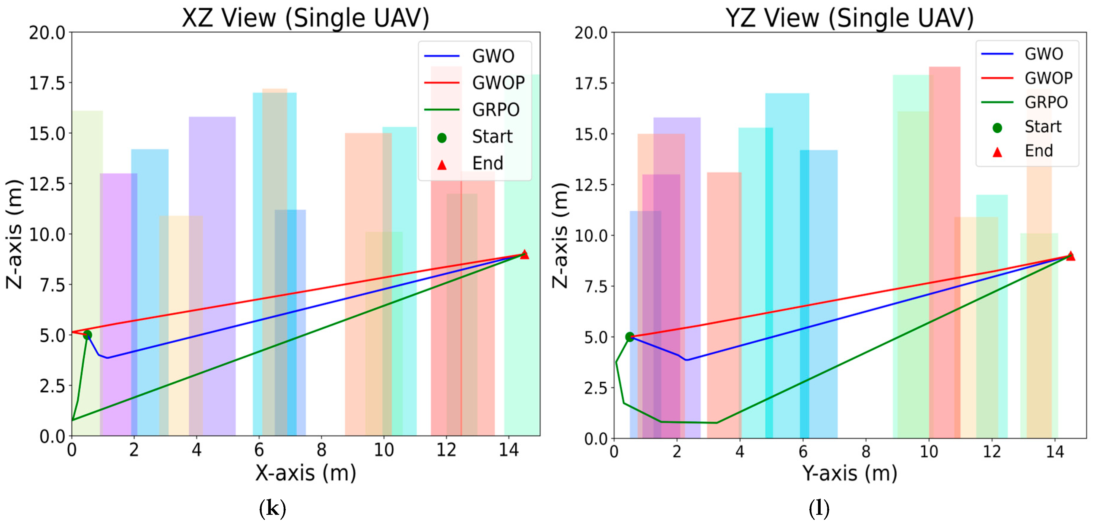
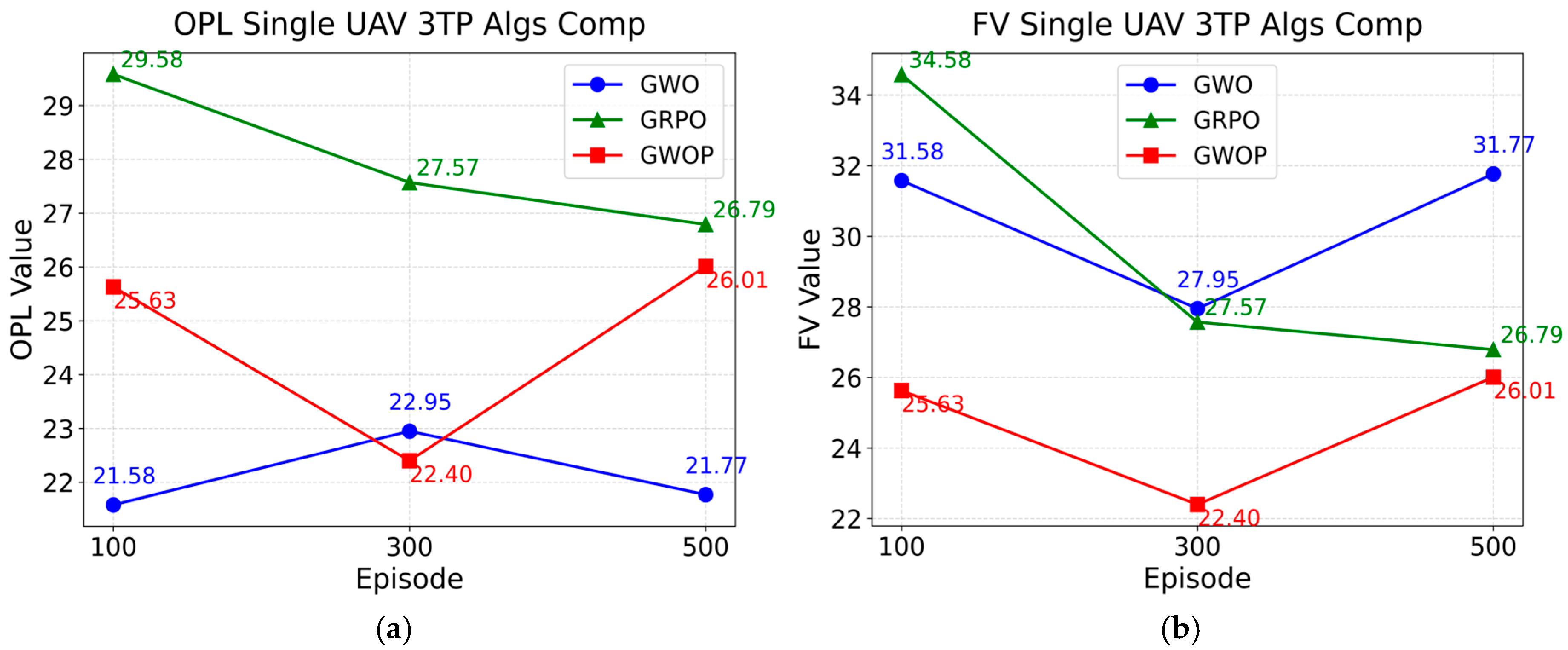
Experiment 1: Due to the limitations of visualization in the actual flight environment, supplementary experiments were carried out in a visualized three-dimensional environment, as illustrated in Figure 9. In this setup, the green circle denotes the starting point of the flight trajectory, the red triangle indicates the target endpoint of the delivery, and the colored columnar structures represent urban buildings acting as obstacles. In each trial, a single unmanned aerial vehicle (UAV) initiated its flight from the starting point and employed the improved GWOP algorithm, the classic GWO algorithm, and the GRPO algorithm, respectively, to navigate around obstacles. The optimal algorithm is defined as the one that reaches the target endpoint first, with a collision-free trajectory and the shortest path length. To ensure experimental reliability, simulations were conducted over 100, 300, and 500 iterations.

Based on the aforementioned three-dimensional environment, the comparison visualization results of a single unmanned aerial vehicle (UAV) operating under three different trajectory planning algorithms indicate that, in the 100-iteration Figure 9a, all trajectory planning algorithms successfully reach the target endpoint and complete the path from the starting point to the destination. However, as shown in Figure 9b–d, the GWOP algorithm generates a generally smoother obstacle-avoidance path, whereas the GWO and GRPO algorithms experience multiple collisions during trajectory planning. The 300-iteration Figure 9e–h and the 500-iteration Figure 9i–l consistently demonstrate that the improved GWOP algorithm significantly outperforms the classical GWO and GRPO algorithms in terms of obstacle avoidance space utilization and path smoothness. The training results of trajectory planning using a single UAV with the three algorithms across 100, 300, and 500 iterations are presented in Figure 10.

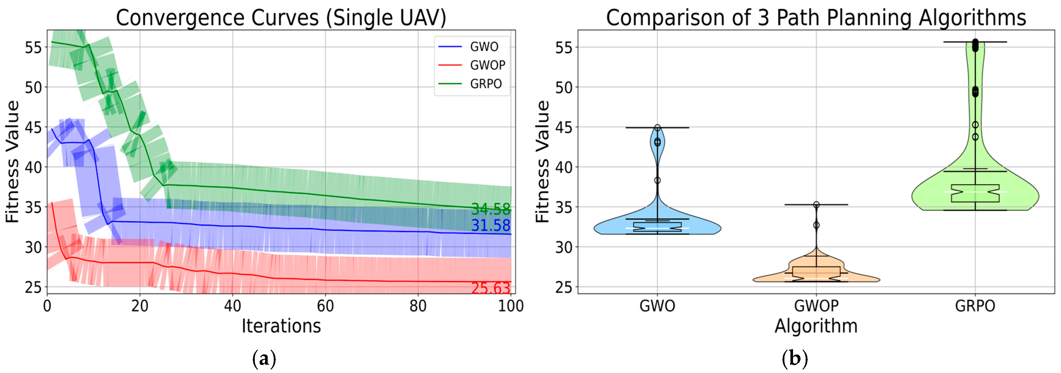
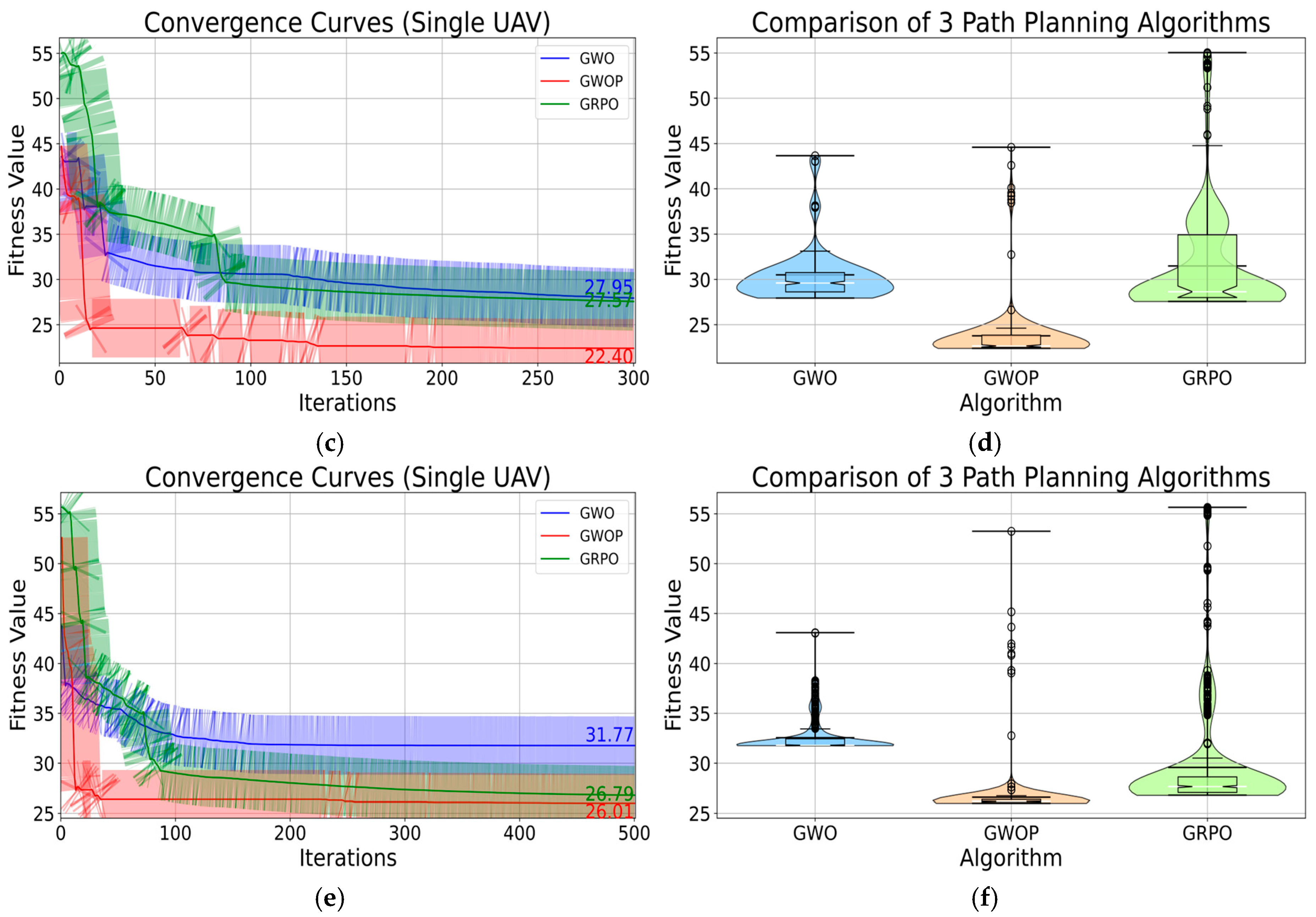
The training results in Figure 10a demonstrate that GWOP achieves rapid convergence within approximately 20 iterations, whereas the GWO and GRPO algorithms exhibit slower initial convergence and only gradually stabilize after around 40 iterations. Consequently, in the 100-iteration experiment, GWOP displays a significantly faster convergence rate compared to GWO and GRPO, reaching the optimal solution with fewer iterations. As shown in Figure 10b, the fitness value of the GWOP algorithm is approximately 25.63, while those of the GWO and GRPO algorithms are 31.58 and 34.58, respectively. This indicates that GWOP incurs lower cost consumption than GWO and GRPO in path planning. Figure 10c,d from the 300-iteration results, as well as Figure 10e,f from the 500-iteration results, further confirm that GWOP converges faster and achieves lower planning costs in trajectory planning.

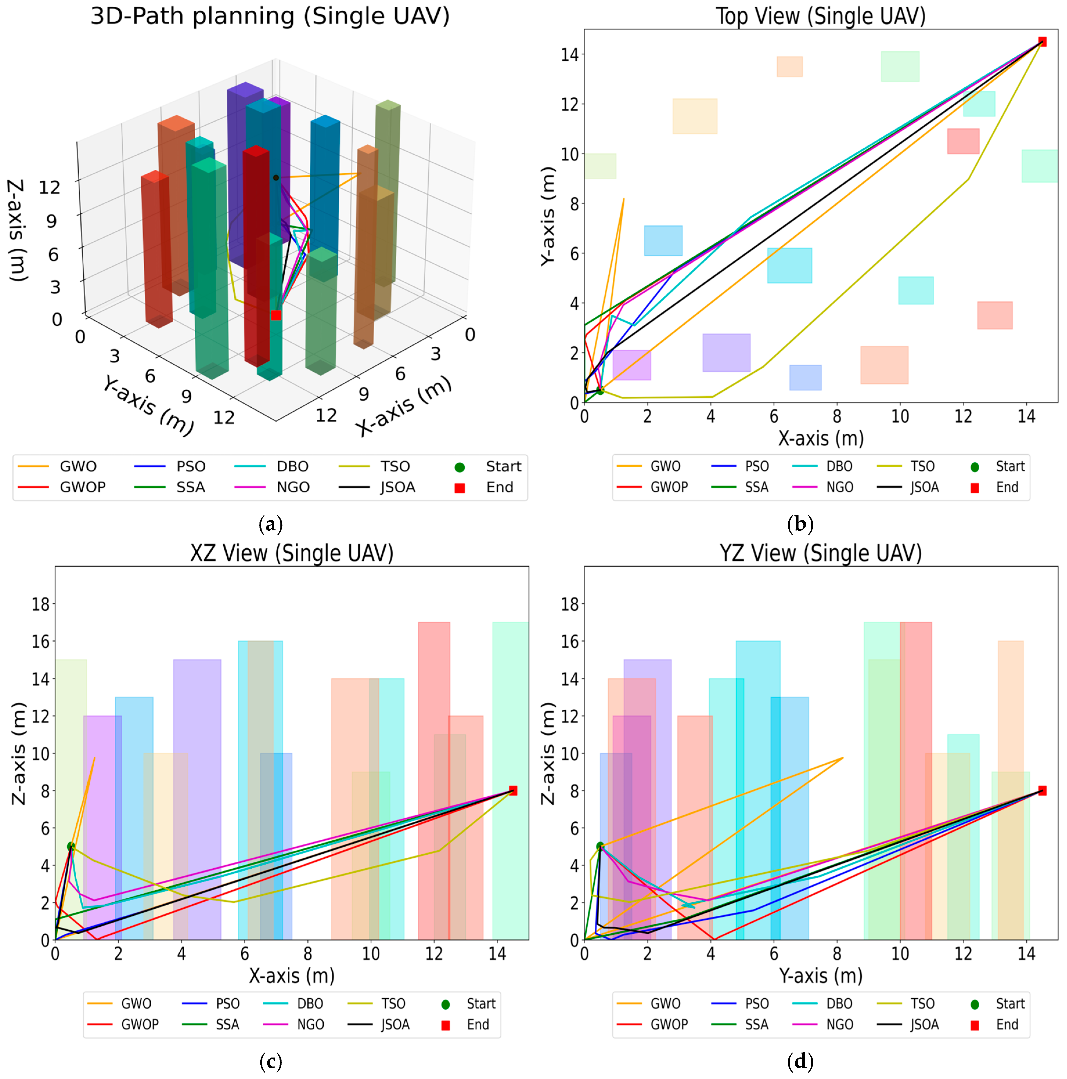
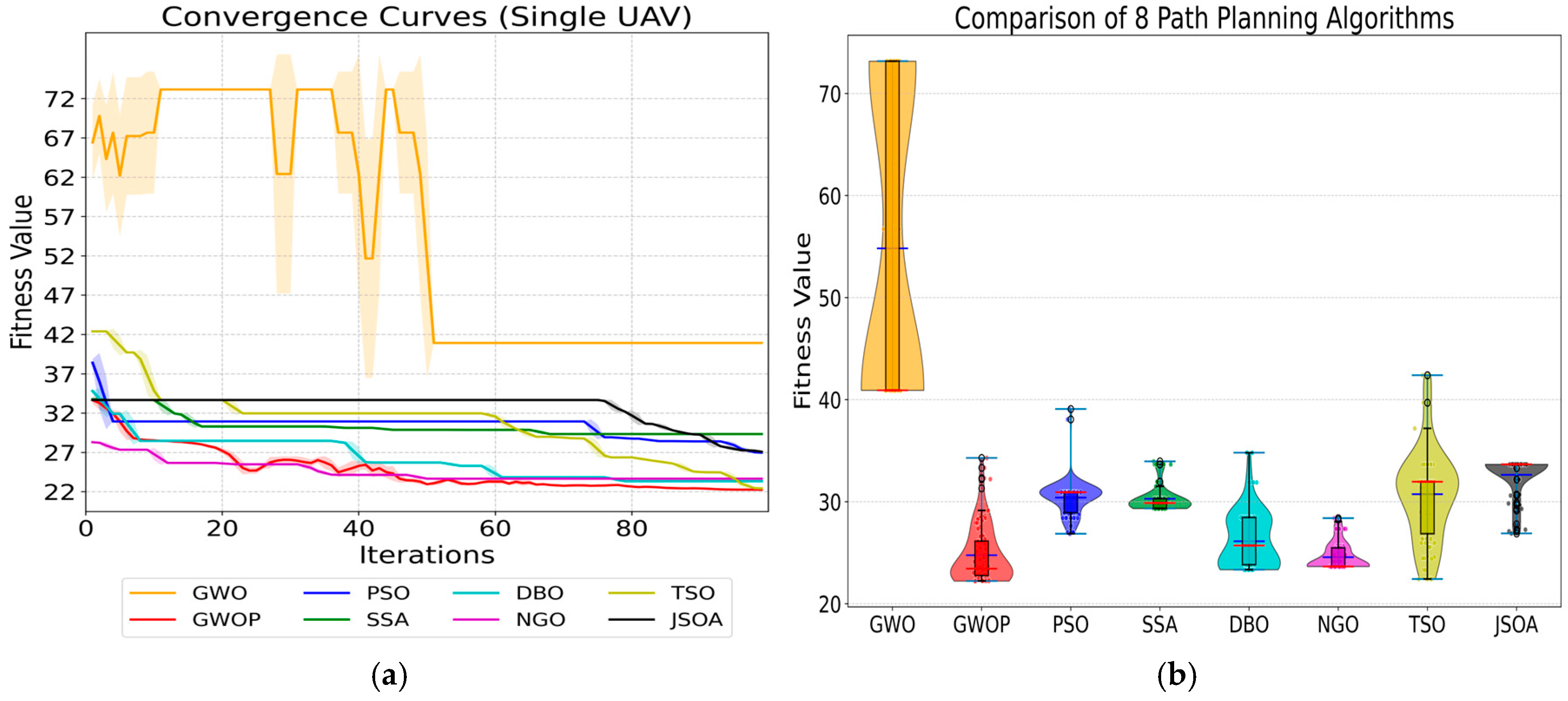
Experiment 2: Given the superior performance of GWOP over GWO observed in the previous experiment, six additional trajectory planning algorithms—PSO, SSA, DBO, NGO, TSO, and JSOA—are included for comparison. A total of eight experiments are conducted for trajectory planning from the starting point to the target endpoint, as illustrated in Figure 11. The starting point, target endpoint, and building obstacles are configured identically to those in Experiment 1.

Based on the visualization results comparing eight different trajectory planning algorithms for a single unmanned aerial vehicle (UAV) in the aforementioned three-dimensional environment, Figure 11a presents the trajectory curves generated by the eight algorithms from the starting point to the target endpoint. The trajectories reveal notable differences among the algorithms. Combined with Figure 11b–d, it is evident that the GWO algorithm frequently encounters obstacles during trajectory planning, whereas the PSO, SSA, and JSOA algorithms produce redundant obstacle avoidance paths. Therefore, it can be concluded that the GWOP algorithm generates a smoother obstacle avoidance trajectory. A further analysis of the data obtained from the eight algorithms is provided in Figure 12.

The training results from the aforementioned Figure 12a indicate that the GWOP algorithm achieves convergence within approximately 20 iterations and subsequently stabilizes. In contrast, the GWO algorithm exhibits significant fluctuations during the first 53 iterations and converges to the highest cost. The DBO and NGO algorithms also converge within about 40 iterations, with relatively lower costs. Meanwhile, the PSO, TSO, SSA, and JSOA algorithms begin to converge after approximately 60 iterations, demonstrating the slowest convergence speed. As shown in Figure 12b, the fitness values of the GWOP algorithm are concentrated between 20 and 30, clearly outperforming the other seven algorithms in terms of fitness.

5.3.2. Comparing Multi-UAV Path Planning Experiments

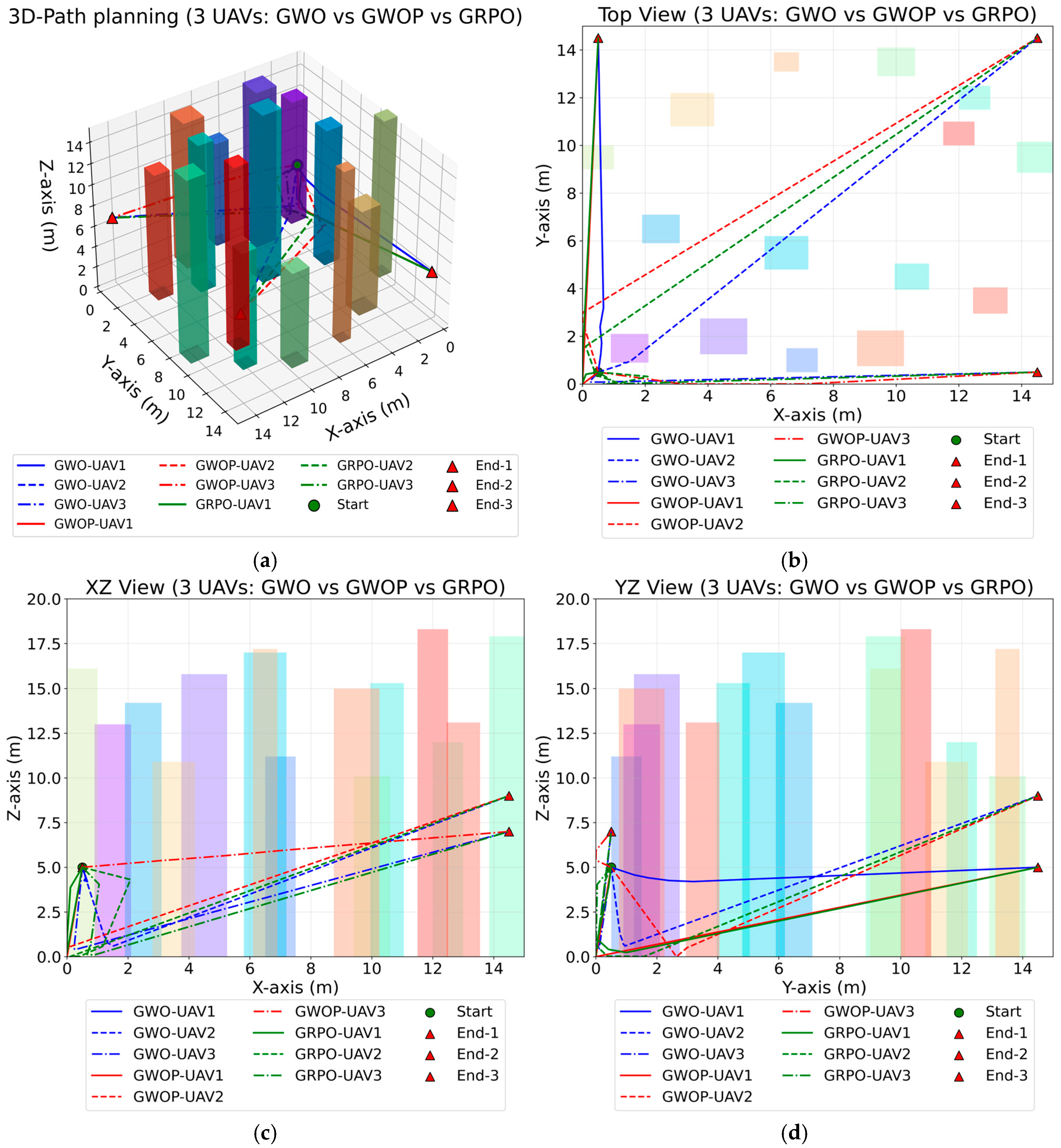
Experiment 3: Following the superior performance of the GWOP algorithm in the previous single UAV three-dimensional trajectory planning experiments, this experiment further introduces multiple UAVs to evaluate the robustness of the improved two-layer GWOP algorithm. The trajectory comparison of the improved GWOP algorithm, the original GWO algorithm, and the GRPO algorithm for multiple UAVs is presented in Figure 13. In this setup, three UAVs share the same departure point but have different target endpoints, with the differently colored columns representing urban building obstacles.

Based on the aforementioned three-dimensional environment, the comparison visualization results of multiple unmanned aerial vehicles (UAVs) operating under three different trajectory planning algorithms demonstrate that, as shown in Figure 13a, all three UAVs using these algorithms exhibit basic obstacle avoidance capabilities and successfully complete the task of planning paths from the starting point to the target. From the top view in Figure 13b, it is evident that the UAVs under the GWOP algorithm achieve smoother obstacle avoidance maneuvers. In contrast, UAVs using the GWO and GRPO algorithms experience collisions with obstacles in certain cases, particularly among UAVs with different serial numbers. Notably, no collision behavior occurs during the trajectory planning of the three UAVs using the GWOP algorithm, which effectively reduces energy consumption and control complexity during flight. By synthesizing the various perspective views of the flight environment, it can be concluded that the improved GWOP algorithm offers significant advantages over the classical GWO and GRPO algorithms in multi-UAV flight scenarios. To validate the reliability of the conclusions drawn from the visualization results, further analysis is conducted on the convergence and violin distribution statistics, as presented in Figure 14.

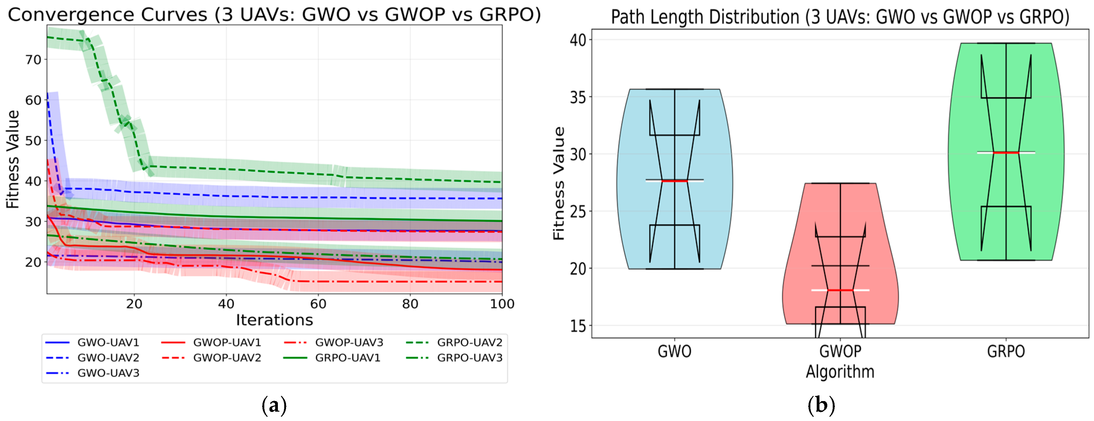
The training results from Figure 14a demonstrate that the GWOP algorithm achieves rapid convergence within 50 iterations for the trajectory planning of three drones. In contrast, UAV2 using the GWO algorithm begins to converge after 5 iterations, while the GRPO algorithm starts to converge after 20 iterations. However, the converged fitness values of both the GWO and GRPO algorithms are higher than those of all drones under the GWOP algorithm. As shown in Figure 14b, the fitness values of the GWOP algorithm are concentrated in the range of 15 to 27, whereas those of the GWO and GRPO algorithms are concentrated in the ranges of 20 to 36 and 21 to 39, respectively. This indicates that the GWOP algorithm outperforms the GWO and GRPO algorithms in terms of the quality of trajectories generated for multiple drones.

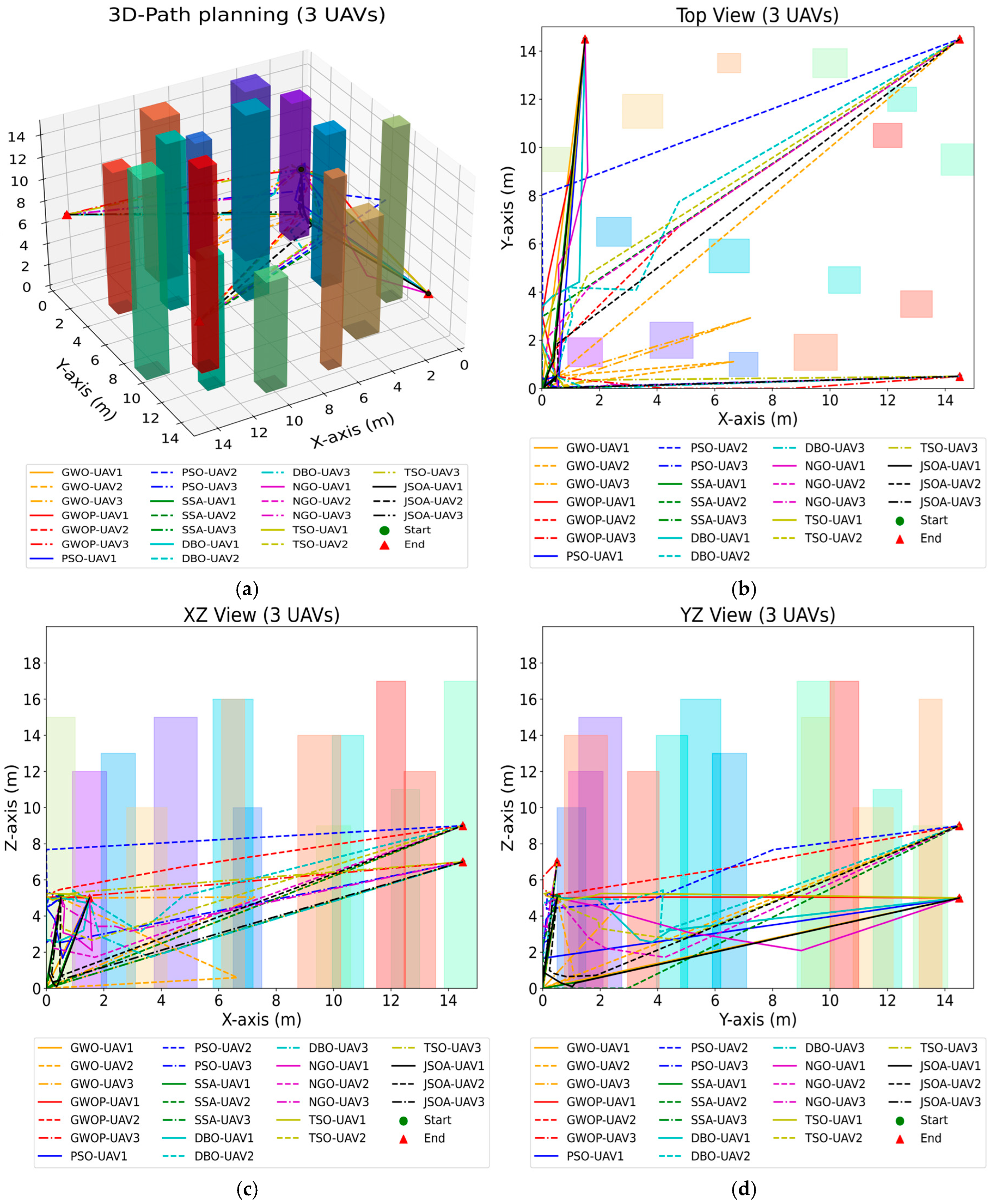
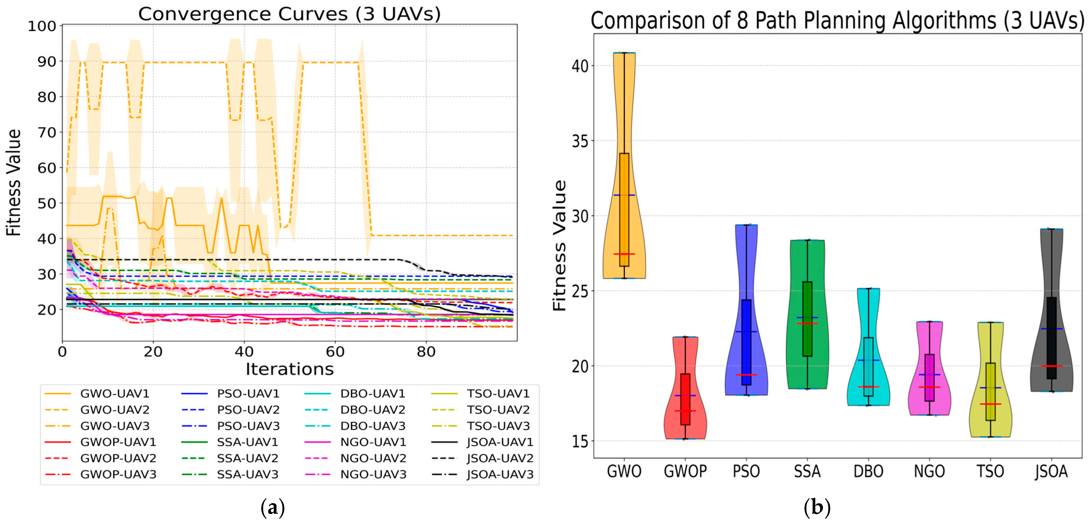
Experiment 4: Given the superior performance of the GWOP algorithm over the GWO algorithm in multi-drone trajectory planning, as demonstrated in the previous results, six additional trajectory planning algorithms—PSO, SSA, DBO, NGO, TSO, and JSOA—are introduced for further comparative analysis, as illustrated in Figure 15. A comparative experiment is conducted using eight different algorithms for trajectory planning from the starting point to the target endpoints. The starting point, building obstacles, and the number of drones remain consistent with those in Experiment 1, while the number of target endpoints is increased to three to match the current number of drones.

From the aforementioned three-dimensional environment involving multiple drones, the visualization results obtained using eight different trajectory planning algorithms demonstrate that, as shown in Figure 15a, all three drones successfully avoid the three-dimensional cylindrical obstacles and reach the target destination using each of the eight algorithms. From the top view in Figure 15b, it is evident that multi-drone operations based on the GWO, TSO, SSA, NGO, and JSOA algorithms exhibit varying degrees of collision. Meanwhile, trajectory planning using the PSO and DBO algorithms results in a local “clustering” phenomenon. In contrast, the GWOP algorithm generates more dispersed trajectories, effectively reducing the “potential conflict risk” in multi-drone collaborative planning. Figure 15c,d further confirm the superior performance of the GWOP algorithm in terms of spatial utilization. To provide a more in-depth evaluation, the convergence characteristics and violin distribution statistics presented in Figure 16 are further analyzed.

The training results from Figure 16a demonstrate that the GWOP algorithm achieves rapid convergence in the trajectory planning of three drones, stabilizing around the 18th iteration. In contrast, the GWO algorithm exhibits significant fluctuations during the first 60 iterations and only stabilizes after the 70th iteration. The DBO and SSA algorithms converge within the first 55 iterations, but their fitness values are notably higher than those of the GWOP algorithm. The TSO, PSO, NGO, and JSOA algorithms converge the slowest, with convergence beginning after the 70th iteration. As shown in Figure 16b, the fitness values of the GWOP algorithm are concentrated in the range of 15 to 22, whereas those of the GWO algorithm fall within the range of 27 to 41. The fitness values of the DBO, NGO, TSO, PSO, SSA, and JSOA algorithms all exceed the range observed for the GWOP algorithm. Therefore, it can be concluded that the GWOP algorithm demonstrates a significant advantage over the other seven algorithms in terms of both convergence speed and trajectory quality in multi-drone trajectory planning.

6. Discussion

6.1. Discussion on the Results of a Single UAV

This section provides a summary and analysis of the results from the aforementioned experimental content. Key metrics are defined as follows: Optimal Path Length (OPL), Average Path Length (APL), Number of Obstacle Collisions (NOC), Fitness Value (FV), Number of UAVs (NOU), Trajectory Planning (TP), Algorithms (Algs), and Comparison (Comp).

In Experiment 1, the GRPO algorithm was integrated with and used to improve the classical GWO algorithm. Subsequently, the enhanced two-layer GWOP algorithm was evaluated through ablation experiments by comparing it with the classical GWO and GRPO algorithms. The trajectory planning of a single unmanned aerial vehicle (UAV) from the starting point to the endpoint was carried out, and the results are summarized in

Table 3. Comp Results Table of 3TP Algs for Single UAV.

Attention Method	Algorithms 1 (GWO)			Algorithms 2 (GRPO)			Algorithms 3 (GWOP)
	100	300	500	100	300	500	100	300	500
OPL/m	21.58	22.95	21.77	29.58	27.57	26.79	25.63	22.40	26.01
NOC/counts	2	1	2	1	0	0	0	0	0
FV	31.58	27.95	31.77	34.58	27.57	26.79	25.63	22.40	26.01

. Specifically, the GWOP, GWO, and GRPO algorithms were each trained 100, 300, and 500 times, respectively, across three evaluation indicators: Optimal Path Length (OPL), Number of Collisions (NOC), and Fitness Value (FV). The results were then summarized and analyzed. An evaluation indicator was considered optimal when the OPL and FV values were minimized and no collisions (NOC = 0) were observed.

Table 3 provides a detailed comparison and analysis of the GWOP algorithm, GWO algorithm, and GRPO algorithm in the context of a single drone’s flight, focusing on the OPL, NOC, and FV indicators. The results are summarized in Figure 17. As shown in Figure 17a, which illustrates the OPL values, the GWO algorithm achieved distances of 21.58 m and 21.77 m at Episode 100 and Episode 300, respectively, which are shorter than the GWOP algorithm’s 25.63 m and 26.01 m at the same episodes. However, the GWO algorithm encountered two collisions in both cases. Regarding the FV indicator in Figure 17b, the GWOP algorithm obtained fitness values of 25.63 m, 22.40 m, and 26.01 m at Episodes 100, 300, and 500, respectively. These values are significantly lower than those of the GWO algorithm (31.58 m, 27.95 m, and 31.77 m) and the GRPO algorithm (34.58 m, 27.57 m, and 26.79 m). Furthermore, as indicated by the NOC metric, the GWOP algorithm successfully avoided obstacles in all three iterations, whereas both the GWO and GRPO algorithms experienced multiple collisions before improvement. These results clearly demonstrate the superior performance of the improved GWOP algorithm in three-dimensional trajectory planning for logistics drones.

From Figure 17, it can be concluded that the improved double-layer fusion GWOP algorithm reduced the FV by 18.84% at 100 iterations, 19.86% at 300 iterations, and 18.13% at 500 iterations, with an average reduction of 18.94% across the three iteration levels compared to the improved GWO algorithm. Compared with the improved GRPO algorithm, the reductions were 25.88%, 18.75%, and 2.91% at 100, 300, and 500 iterations, respectively, yielding an average reduction of 15.85%.

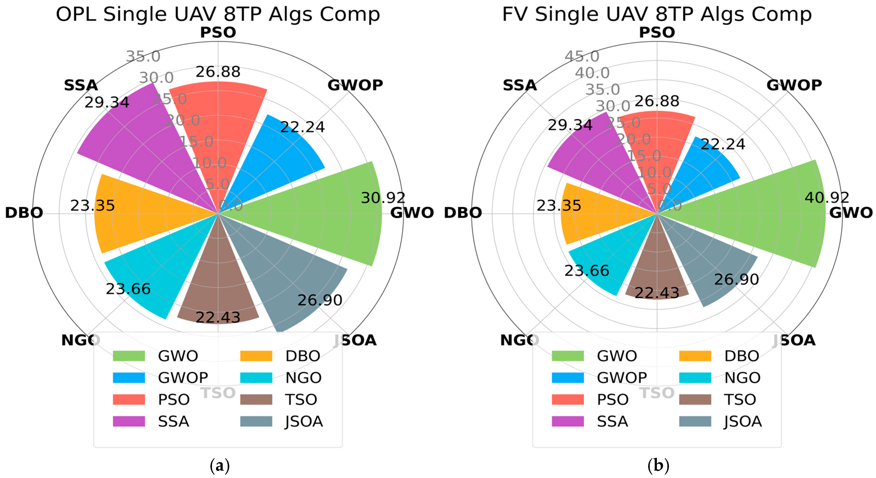
In Experiment 2, the GWOP algorithm demonstrated significantly better performance than the GWO and GRPO algorithms in single UAV trajectory planning. To further evaluate the improved GWOP algorithm, six additional trajectory planning algorithms were introduced, and a comparative analysis was conducted using a total of eight different algorithms. Finally, experiments with 100 iterations were carried out for OPL, NOC, and FV, and the results are summarized in

Table 4. Comp Results Table of 8TP Algs for Single UAV.

Algorithm	OPL/m	NOC/Counts	FV
GWO	30.92	5	40.92
GWOP	22.24	0	22.24
PSO	26.88	0	26.88
SSA	29.34	0	29.34
DBO	23.35	0	23.35
NGO	23.66	0	23.66
TSO	22.43	0	22.43
JSOA	26.90	0	26.90

.

Table 4 presents a detailed comparison and analysis of the GWOP algorithm against seven other algorithms—GWO, PSO, SSA, DBO, NGO, TSO, and JSOA—in the single-drone flight scenario, focusing on the OPL, NOC, and FV metrics. The results are illustrated in Figure 18. As shown in Figure 18a, the GWOP algorithm achieves a trajectory length of 22.24 m, whereas the other seven algorithms yield trajectory lengths of 30.92 m, 26.88 m, 29.34 m, 23.35 m, 23.66 m, 22.43 m, and 26.90 m, respectively. According to Figure 18b, the GWOP algorithm obtains a fitness value of 22.24 for the FV metric, while the corresponding values for the other algorithms are 40.92, 26.88, 29.34, 23.35, 23.66, 22.43, and 26.90. Regarding the NOC data, the trajectories generated by the GWOP, PSO, DBO, NGO, and TSO algorithms satisfy the collision-free requirement in the single-drone delivery task. Overall, the experimental results indicate that the GWOP algorithm outperforms all other tested algorithms.

From Figure 18a, it can be observed that the improved two-layer fused GWOP algorithm achieves an OPL value that is 15.15% lower than the average of the other seven algorithms. As shown in Figure 18b, the improved GWOP algorithm also demonstrates a 19.54% reduction in FV compared to the average of the other algorithms. In summary, these results indicate that the improved two-layer GWOP algorithm offers significant advantages in single UAV trajectory planning.

6.2. Discussion on the Results of Multiple UAVs

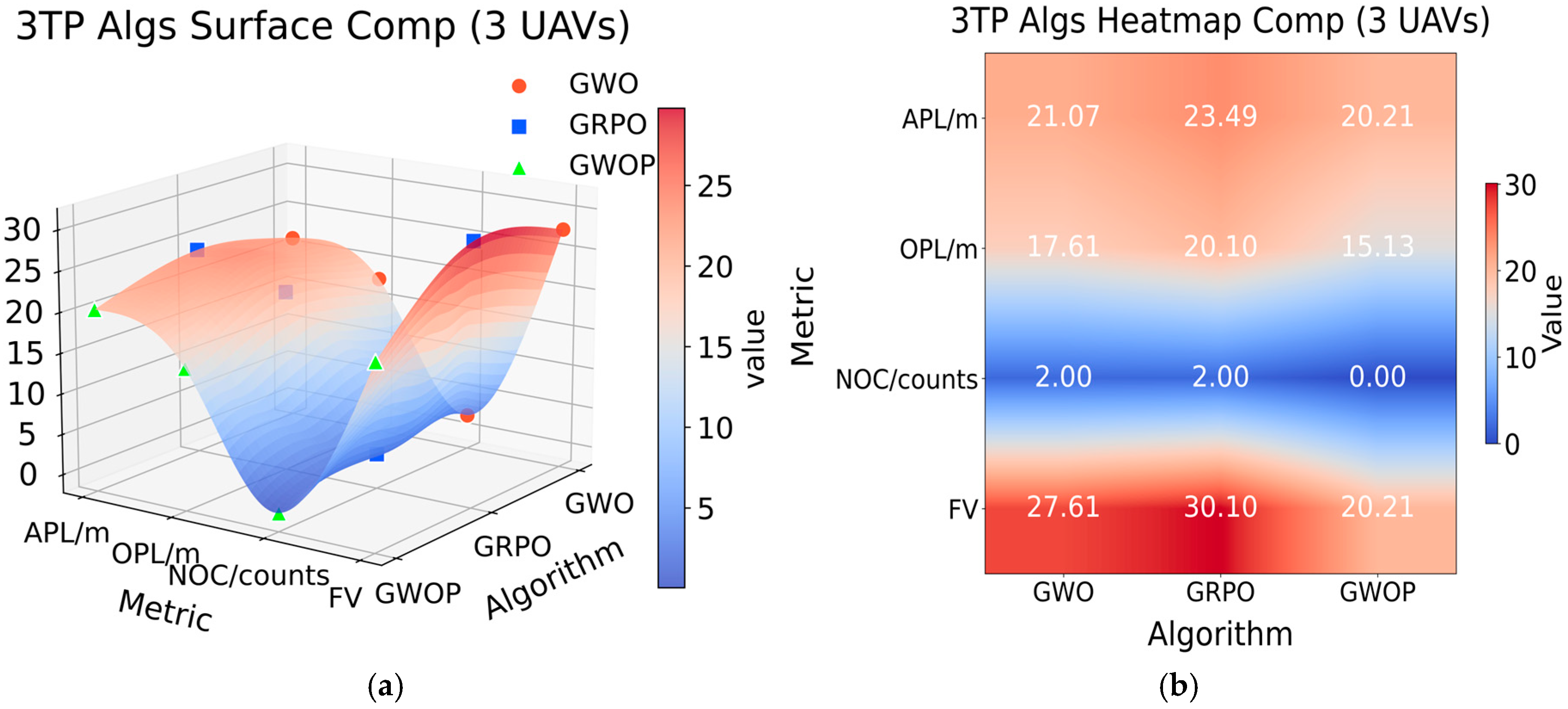
In Experiment 3, after verifying the superiority of the GWOP algorithm over multiple algorithms in the single UAV scenario, the number of UAVs was increased to evaluate its performance in a multi-UAV setting. The improved two-layer fused GWOP algorithm was compared with the classic GWO and GRPO algorithms in this multi-UAV scenario. The trajectory planning data from the starting point to the endpoint for multiple UAVs are presented in

Table 5. Comp Results Table of 3TP Algs for Multi-UAVs.

Algorithm	APL/m	OPL/m	NOC/Counts	FV
GWO	21.07	17.61	2	27.61
GRPO	23.49	20.10	2	30.10
GWOP	20.21	15.13	0	20.21

. Specifically, 100 iterations were conducted for each of the four evaluation indicators—APL, OPL, NOC, and FV—for the GWOP, GWO, and GRPO algorithms. The evaluation criteria consider APL, OPL, and FV optimal when their values are minimized, and NOC is zero, indicating no collisions.

Table 5 presents the APL, OPL, NOC, and FV index data obtained from the flight trajectories of multiple drones using the GWOP, GWO, and GRPO algorithms. The data were visualized and analyzed, resulting in Figure 19. As shown in Figure 19a,b, the GWOP algorithm achieves APL, OPL, and FV values of 20.21 m, 15.13 m, and 20.21 m, respectively, which are significantly lower than the corresponding values for the GWO algorithm (21.07 m, 17.61 m, and 27.61 m) and the GRPO algorithm (23.49 m, 20.10 m, and 30.10 m). Moreover, the GWOP algorithm successfully completed conflict-free obstacle avoidance in the trajectory planning of three drones, whereas both the GWO and GRPO algorithms resulted in two collision incidents. Therefore, the experimental results demonstrate that the GWOP algorithm exhibits a clear advantage over the GWO and GRPO algorithms in multi-drone trajectory planning.

From Figure 19a,b, it can be observed that the improved double-layer fusion GWOP algorithm reduces the APL index by 4.08% compared to the GWO algorithm, the OPL index by 14.08%, and the FV index by 26.80%. Compared with the GRPO algorithm, the reductions are 13.96% for APL, 24.73% for OPL, and 32.86% for FV. These results further confirm the effectiveness of the improved GWOP algorithm in multi-UAV trajectory planning.

In Experiment 4, after demonstrating the superiority of the GWOP algorithm over two other algorithms in the multi-UAV scenario, six additional trajectory planning algorithms were introduced. A comparative analysis involving a total of eight algorithms was then conducted in the 3D multi-UAV trajectory planning environment to further validate the performance of the improved GWOP algorithm. The experimental results from 100 iterations for APL, OPL, NOC, and FV are summarized in

Table 6. Comp Results Table of 8TP Algs for Multi-UAVs.

Algorithm	APL/m	OPL/m	NOC/Counts	FV
GWO	38.51	32.03	6	31.37
GWOP	17.35	15.00	0	18.02
PSO	21.61	16.05	6	22.27
SSA	22.55	18.47	2	23.22
DBO	19.70	16.61	0	20.37
NGO	18.74	16.57	1	19.41
TSO	17.87	15.26	1	18.54
JSOA	21.13	16.30	2	22.46

. The evaluation criteria consider the shortest APL, OPL, and FV values as optimal, provided that no NOC occur.

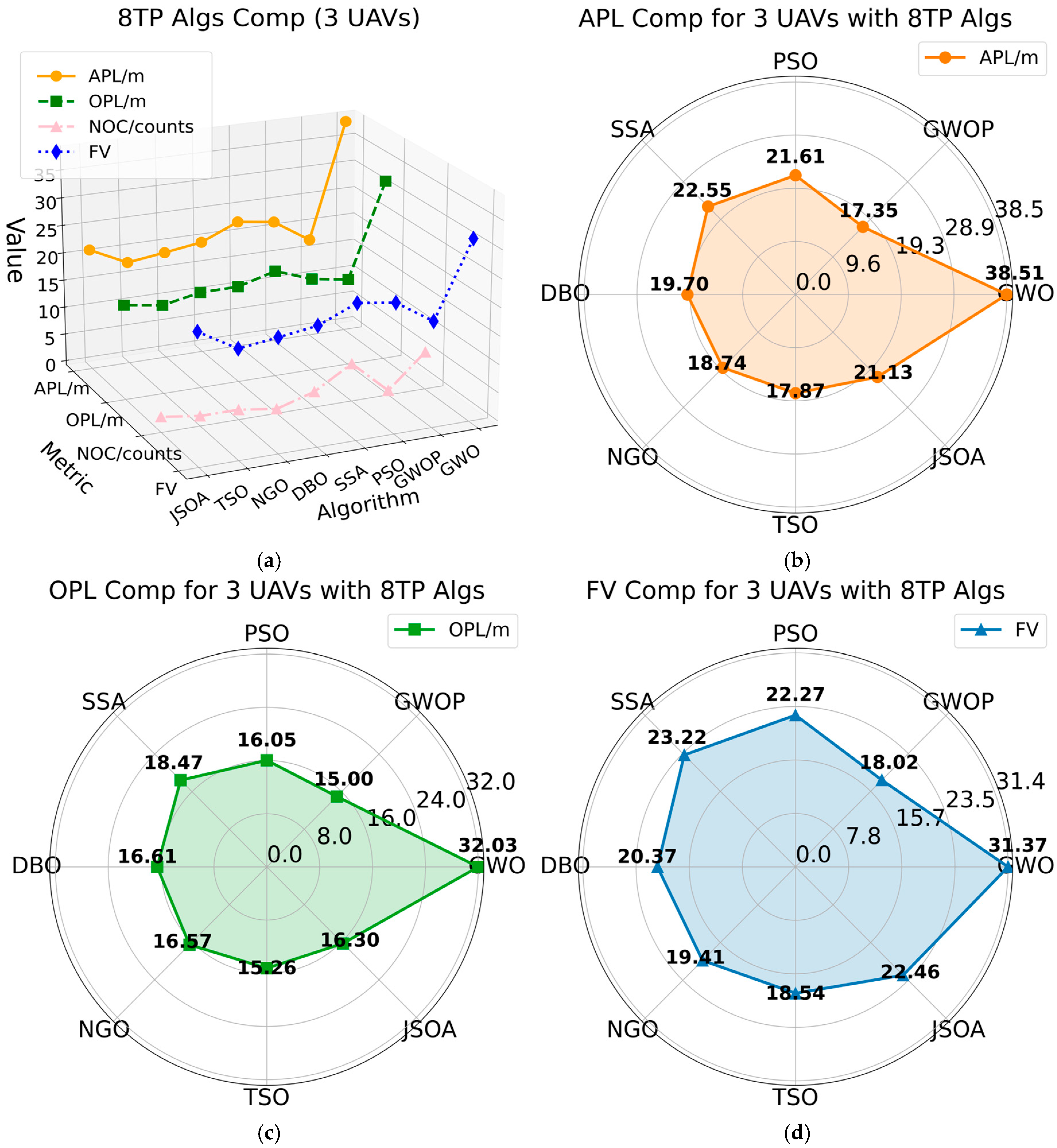
Table 6 presents a detailed comparison and analysis of the GWOP algorithm against seven other algorithms—GWO, PSO, SSA, DBO, NGO, TSO, and JSOA—in the context of multiple drone flights, focusing on the APL, OPL, NOC, and FV metrics. The results are illustrated in Figure 20. According to the APL data in Figure 20b, the GWOP algorithm achieves a trajectory length of 17.35 m, whereas the other seven algorithms yield lengths of 38.51 m, 21.61 m, 22.55 m, 19.70 m, 18.74 m, 17.87 m, and 21.13 m, respectively. As shown in Figure 20c, the OPL value for the GWOP algorithm is 15.00 m, compared to 32.03 m, 16.05 m, 18.47 m, 16.61 m, 16.57 m, 15.26 m, and 16.30 m for the other algorithms. Regarding the FV metric in Figure 20d, the GWOP algorithm obtains a value of 18.02 m, while the corresponding values for the other algorithms are 31.37 m, 22.27 m, 23.22 m, 20.37 m, 19.41 m, 18.54 m, and 22.46 m. Finally, as indicated in Figure 20a, the GWO algorithm demonstrates a significant advantage over the other seven algorithms in terms of APL, OPL, NOC, and FV metrics in multi-drone trajectory planning.

To summarize, as indicated in Figure 20a, the improved two-layer fusion GWOP algorithm demonstrates superior performance compared to the other seven algorithms. Specifically, it achieves an APL index that is 24.14% lower than the average, an OPL index that is 20.04% lower, and an FV index that is 19.98% lower. Furthermore, the trajectory curve generated by the GWOP algorithm for path planning from the starting point to the target endpoint satisfies the requirements of an optimal, conflict-free trajectory.

7. Conclusions

This study addresses the challenges of dynamic trajectory planning for unmanned aerial vehicles (UAVs) in logistics environments. First, a three-dimensional multi-objective flight model is established. Based on this framework, a two-layer fusion GWOP algorithm is proposed. Subsequently, the GAT attention mechanism is integrated to enable dynamic association. The key experimental findings are summarized as follows:

• The CEC2017 benchmark functions are employed for evaluation. Compared with the GWO algorithm, the improved two-layer fusion GWOP algorithm demonstrates superior convergence curves and fitness values across unimodal, multimodal, and complex functions F1–F10. When compared with six other algorithms—PSO, SSA, DBO, NGO, TSO, and JSOA—it achieves better fitness values in the hybrid functions F11–F20 and F21–F25.
• In the single UAV 3D trajectory planning experiment, the improved GWOP algorithm reduces the FV (fitness value) by 18.84%, 19.86%, and 18.13% at 100, 300, and 500 iterations, respectively, yielding an average reduction of 18.94% across all three. The NOC (number of collisions) is reduced from 2 to 0. Compared with the classic GRPO algorithm, the FV reductions are 25.88%, 18.75%, and 2.91% at the same iteration levels, with an average reduction of 15.85%, and the NOC is reduced from 1 to 0. These results highlight the algorithm’s superior path optimization capability and robust obstacle avoidance performance.
• When extended to a comparison involving eight trajectory planning algorithms, the GWOP algorithm achieves OPL (optimal path length) and FV values that are 15.15% and 19.54% lower than the average, respectively, further confirming its effectiveness in complex 3D trajectory planning for single UAVs.
• In the multi-UAV 3D scenario, the advantages of the GWOP algorithm become even more pronounced. Compared with the GWO algorithm, it reduces APL (average path length), OPL, and FV by 4.08%, 14.08%, and 26.80%, respectively. Compared with the GRPO algorithm, the reductions are 13.96%, 24.73%, and 32.86%, respectively. The NOC is also reduced from 2 to 0, further validating the algorithm’s superior obstacle avoidance and trajectory optimization capabilities.
• When evaluated against eight algorithms in a multi-UAV environment, the GWOP algorithm shows reductions of 24.14% in APL (average path length), 20.04% in OPL (optimal path length), and 19.98% in FV (fitness value) compared to the average. Collectively, these experiments demonstrate that the improved GWOP algorithm consistently outperforms other methods in terms of path length, obstacle avoidance, and trajectory smoothness, offering an efficient and reliable planning solution for UAV logistics operations.

Despite its strong performance, future research can further enhance the algorithm in three key directions:

First, improving adaptability to meteorological conditions by incorporating real-time weather data—such as wind intensity and rainfall—to better simulate real-world logistics uncertainties.

Second, expanding to large-scale UAV clusters to explore the algorithm’s scalability in coordinating dozens or even hundreds of UAVs, optimizing communication and path coordination mechanisms for complex swarm logistics tasks.

Third, extending the algorithm to cross-platform and multi-objective optimization, enabling its application in heterogeneous logistics systems such as autonomous ground vehicles and unmanned ships. This would involve integrating constraints like energy consumption and time windows, ultimately supporting the development of a globally coordinated intelligent logistics path planning system and advancing the evolution of the smart logistics ecosystem.

References

1. Niu, B.; Zhang, J.; Xie, F. Drone logistics’ resilient development: Impacts of consumer choice, competition, and regulation. Transp. Res. Part A Policy Pract. 2024, 185, 104126. [Google Scholar] [CrossRef]
2. Shang, Z.; Bradley, J.; Shen, Z. A co-optimal coverage path planning method for aerial scanning of complex structures. Expert Syst. Appl. 2020, 158, 113535. [Google Scholar] [CrossRef]
3. Liu, X.; Li, G.; Yang, H.; Zhang, N.; Wang, L.; Shao, P. Agricultural UAV trajectory planning by incorporating multi-mechanism improved grey wolf optimization algorithm. Expert Syst. Appl. 2023, 233, 120946. [Google Scholar] [CrossRef]
4. Zhang, C.; Zhou, W.; Qin, W.; Tang, W. A novel UAV path planning approach: Heuristic crossing search and rescue optimization algorithm. Expert Syst. Appl. 2023, 215, 119243. [Google Scholar] [CrossRef]
5. Solka, J.L.; Perry, J.C.; Poellinger, B.R.; Rogers, G.W. Fast computation of optimal paths using a parallel Dijkstra algorithm with embedded constraints. Neurocomputing 1995, 8, 195–212. [Google Scholar] [CrossRef]
6. Phong, T.Q.; Hoai An, L.T.; Tao, P.D. Decomposition branch and bound method for globally solving linearly constrained indefinite quadratic minimization problems. Oper. Res. Lett. 1995, 17, 215–220. [Google Scholar] [CrossRef]
7. Huang, J.; Chen, C.; Shen, J.; Liu, G.; Xu, F. A self-adaptive neighborhood search A-star algorithm for mobile robots global path planning. Comput. Electr. Eng. 2025, 123, 110018. [Google Scholar] [CrossRef]
8. Wang, J.; Bi, C.; Liu, F.; Shan, J. Dubins-RRT* motion planning algorithm considering curvature-constrained path optimization. Expert Syst. Appl. 2026, 296, 128390. [Google Scholar] [CrossRef]
9. Yu, X.; Jiang, N.; Wang, X.; Li, M. A hybrid algorithm based on grey wolf optimizer and differential evolution for UAV path planning. Expert Syst. Appl. 2023, 215, 119327. [Google Scholar] [CrossRef]
10. Lou, T.; Yue, Z.; Jiao, Y.; He, Z. A hybrid strategy-based GJO algorithm for robot path planning. Expert Syst. Appl. 2024, 238, 121975. [Google Scholar] [CrossRef]
11. Cui, Y.; Hu, W.; Rahmani, A. A reinforcement learning based artificial bee colony algorithm with application in robot path planning. Expert Syst. Appl. 2022, 203, 117389. [Google Scholar] [CrossRef]
12. Wang, Y.; Tong, K.; Fu, C.; Wang, Y.; Li, Q.; Wang, X.; He, Y.; Xu, L. Hybrid path planning algorithm for robots based on modified golden jackal optimization method and dynamic window method. Expert Syst. Appl. 2025, 282, 127808. [Google Scholar] [CrossRef]
13. Lyu, L.; Yang, F. MMPA: A modified marine predator algorithm for 3D UAV path planning in complex environments with multiple threats. Expert Syst. Appl. 2024, 257, 124955. [Google Scholar] [CrossRef]
14. Xiao, Z.; Li, P.; Liu, C.; Gao, H.; Wang, X. MACNS: A generic graph neural network integrated deep reinforcement learning based multi-agent collaborative navigation system for dynamic trajectory planning. Inf. Fusion 2024, 105, 102250. [Google Scholar] [CrossRef]
15. Yu, X.; Luo, W. Reinforcement learning-based multi-strategy cuckoo search algorithm for 3D UAV path planning. Expert Syst. Appl. 2023, 223, 119910. [Google Scholar] [CrossRef]
16. Popović, M.; Ott, J.; Rückin, J.; Kochenderfer, M.J. Learning-based methods for adaptive informative path planning. Robot. Auton. Syst. 2024, 179, 104727. [Google Scholar] [CrossRef]
17. Fan, Q.; Huang, H.; Li, Y.; Han, Z.; Hu, Y.; Huang, D. Beetle antenna strategy based grey wolf optimization. Expert Syst. Appl. 2021, 165, 113882. [Google Scholar] [CrossRef]
18. Tang, H.; Sun, W.; Lin, A.; Xue, M.; Zhang, X. A GWO-based multi-robot cooperation method for target searching in unknown environments. Expert Syst. Appl. 2021, 186, 115795. [Google Scholar] [CrossRef]
19. Li, K.; Ge, F.; Han, Y.; Wang, Y.A.; Xu, W. Path planning of multiple UAVs with online changing tasks by an ORPFOA algorithm. Eng. Appl. Artif. Intell. 2020, 94, 103807. [Google Scholar] [CrossRef]
20. Niu, Y.; Yan, X.; Wang, Y.; Niu, Y. 3D real-time dynamic path planning for UAV based on improved interfered fluid dynamical system and artificial neural network. Adv. Eng. Inform. 2024, 59, 102306. [Google Scholar] [CrossRef]
21. Lee, H. Research on multi-functional logistics intelligent Unmanned Aerial Vehicle. Eng. Appl. Artif. Intell. 2022, 116, 105341. [Google Scholar] [CrossRef]
22. Yu, S.; Chen, J.; Liu, G.; Tong, X.; Sun, Y. SOF-RRT*: An improved path planning algorithm using spatial offset sampling. Eng. Appl. Artif. Intell. 2023, 126, 106875. [Google Scholar] [CrossRef]
23. Fang, W.; Liao, Z.; Bai, Y. Improved ACO algorithm fused with improved Q-Learning algorithm for Bessel curve global path planning of search and rescue robots. Robot. Auton. Syst. 2024, 182, 104822. [Google Scholar] [CrossRef]
24. Liu, X.; Shao, P.; Li, G.; Ye, L.; Yang, H. Complex hilly terrain agricultural UAV trajectory planning driven by Grey Wolf Optimizer with interference model. Appl. Soft Comput. 2024, 160, 111710. [Google Scholar] [CrossRef]
25. Wang, Z.; Yuan, F.; Li, R.; Zhang, M.; Luo, X. Hidden AS link prediction based on random forest feature selection and GWO-XGBoost model. Comput. Netw. 2025, 262, 111164. [Google Scholar] [CrossRef]
26. Zhu, C.; Bouteraa, Y.; Khishe, M.; Martín, D.; Hernando-Gallego, F.; Vaiyapuri, T. Enhancing unmanned marine vehicle path planning: A fractal-enhanced chaotic grey wolf and differential evolution approach. Knowl.-Based Syst. 2025, 317, 113481. [Google Scholar] [CrossRef]
27. Zhang, L.; Yang, H.; Yang, C.; Zhang, J.; Wang, J. Optimal design of mixed dielectric coaxial-annular TSV using GWO algorithm based on artificial neural network. Integration 2024, 97, 102205. [Google Scholar] [CrossRef]
28. Lakzaei, B.; Haghir Chehreghani, M.; Bagheri, A. LOSS-GAT: Label propagation and one-class semi-supervised graph attention network for fake news detection. Appl. Soft Comput. 2025, 174, 112965. [Google Scholar] [CrossRef]
29. Stamatopoulos, M.; Banerjee, A.; Nikolakopoulos, G. Conflict-free optimal motion planning for parallel aerial 3D printing using multiple UAVs. Expert Syst. Appl. 2024, 246, 123201. [Google Scholar] [CrossRef]
30. Kim, M.; Jang, Y.; Sung, T. Graph-based technology recommendation system using GAT-NGCF. Expert Syst. Appl. 2025, 288, 128240. [Google Scholar] [CrossRef]
31. Zhang, H.; An, X.; He, Q.; Yao, Y.; Zhang, Y.; Fan, F.; Teng, Y. Quadratic graph attention network (Q-GAT) for robust construction of gene regulatory network. Neurocomputing 2025, 631, 129635. [Google Scholar] [CrossRef]
32. Zhao, J.; Yan, Z.; Zhou, Z.; Chen, X.; Wu, B.; Wang, S. A ship trajectory prediction method based on GAT and LSTM. Ocean Eng. 2023, 289, 116159. [Google Scholar] [CrossRef]
33. Zhou, L.; Wang, H. MST-GAT: A multi-perspective spatial-temporal graph attention network for multi-sensor equipment remaining useful life prediction. Inf. Fusion 2024, 110, 102462. [Google Scholar] [CrossRef]
34. Sheng, Z.; Song, T.; Song, J.; Liu, Y.; Ren, P. Bidirectional rapidly exploring random tree path planning algorithm based on adaptive strategies and artificial potential fields. Eng. Appl. Artif. Intell. 2025, 148, 110393. [Google Scholar] [CrossRef]
35. Niu, Y.; Yan, X.; Wang, Y.; Niu, Y. Three-dimensional UCAV path planning using a novel modified artificial ecosystem optimizer. Expert Syst. Appl. 2023, 217, 119499. [Google Scholar] [CrossRef]
36. Fu, B.; Chen, Y.; Quan, Y.; Zhou, X.; Li, C. Bidirectional artificial potential field-based ant colony optimization for robot path planning. Robot. Auton. Syst. 2025, 183, 104834. [Google Scholar] [CrossRef]
37. Stache, F.; Westheider, J.; Magistri, F.; Stachniss, C.; Popović, M. Adaptive path planning for UAVs for multi-resolution semantic segmentation. Robot. Auton. Syst. 2023, 159, 104288. [Google Scholar] [CrossRef]
38. Lin, H.; Shodiq, M.A.F.; Hsieh, M.F. Robot path planning based on three-dimensional artificial potential field. Eng. Appl. Artif. Intell. 2025, 144, 110127. [Google Scholar] [CrossRef]
39. Xia, Q.; Liu, S.; Guo, M.; Wang, H.; Zhou, Q.; Zhang, X. Multi-UAV trajectory planning using gradient-based sequence minimal optimization. Robot. Auton. Syst. 2021, 137, 103728. [Google Scholar] [CrossRef]
40. Hu, L.; Wei, C.; Yin, L. MAPPO-ITD3-IMLFQ algorithm for multi-mobile robot path planning. Adv. Eng. Inform. 2025, 65, 103398. [Google Scholar] [CrossRef]
41. Lin, S.; Liu, A.; Wang, J.; Kong, X. An improved fault-tolerant cultural-PSO with probability for multi-AGV path planning. Expert Syst. Appl. 2024, 237, 121510. [Google Scholar] [CrossRef]
42. Zhang, T.; Hu, H.; Liang, Y.; Liu, X.; Rong, Y.; Wu, C.; Zhang, G.; Huang, Y. A novel path planning approach to minimize machining time in laser machining of irregular micro-holes using adaptive discrete grey wolf optimizer. Comput. Ind. Eng. 2024, 193, 110320. [Google Scholar] [CrossRef]
43. Ou, J.; Hong, S.H.; Song, G.; Wang, Y. Hybrid path planning based on adaptive visibility graph initialization and edge computing for mobile robots. Eng. Appl. Artif. Intell. 2023, 126, 107110. [Google Scholar] [CrossRef]
44. Wang, X.; Zhuang, Y.; Cao, X.; Huai, J.; Zhang, Z.; Zheng, Z.; El-Sheimy, N. GAT-LSTM: A feature point management network with graph attention for feature-based visual SLAM in dynamic environments. Isprs J. Photogramm. 2025, 224, 75–93. [Google Scholar] [CrossRef]
45. Wei, D.; Chen, D.; Huang, Z.; Li, T. An improved chaotic GWO-LGBM hybrid algorithm for emotion recognition. Biomed. Signal Proces. 2024, 98, 106768. [Google Scholar] [CrossRef]
46. Jiang, W.; Lyu, Y.; Li, Y.; Guo, Y.; Zhang, W. UAV path planning and collision avoidance in 3D environments based on POMPD and improved grey wolf optimizer. Aerosp. Sci. Technol. 2022, 121, 107314. [Google Scholar] [CrossRef]
47. Chintam, P.; Lei, T.; Osmanoglu, B.; Wang, Y.; Luo, C. Informed sampling space driven robot informative path planning. Robot. Auton. Syst. 2024, 175, 104656. [Google Scholar] [CrossRef]
48. Xiong, Y.; Zhou, Y.; She, J.; Yu, A. Collaborative coverage path planning for UAV swarm for multi-region post-disaster assessment. Veh. Commun. 2025, 53, 100915. [Google Scholar] [CrossRef]
Figure 1. GWO algorithm framework.
Drones 09 00671 g001
Figure 2. GRPO algorithm framework.
Drones 09 00671 g002
Figure 3. Double-Layer GWOP fusion algorithm framework.
Drones 09 00671 g003
Figure 4. Trajectory Planning and Delivery Process of Logistics UAV: (a) Load letter cargo; (b) Vertical Takeoff; (c) Waypoint 1; (d) Waypoint 2; (e) Waypoint 3; (f) Waypoint 4.
Drones 09 00671 g004
Figure 5. CEC2017 test results.
Drones 09 00671 g005
Figure 6. Experimental Procedure of the Double-Layer Fusion GWOP Algorithm.
Drones 09 00671 g006
Figure 7. Flight turn angle constraint.
Drones 09 00671 g007
Figure 8. Flight altitude constraint diagram.
Drones 09 00671 g008
Figure 9. Comparative Experiment of 2 Algorithms for Single UAV Path Planning: (a) 3D-Path planning Single UAV (100); (b) Top View Single UAV (100); (c) XZ View Single UAV (100); (d) YZ View Single UAV (100); (e) 3D-Path planning Single UAV (300); (f) Top View Single UAV (300); (g) XZ View Single UAV (300); (h) YZ View Single UAV (300); (i) 3D-Path planning Single UAV (500); (j) Top View Single UAV (500); (k) XZ View Single UAV (500); (l) YZ View Single UAV (500).
Drones 09 00671 g009aDrones 09 00671 g009bDrones 09 00671 g009c
Figure 10. Statistical Comparison of 3 Algorithms for Single UAV Path Planning: (a) Convergence Curves Single UAV (100); (b) Comparison 2 Path Planning Algorithms (100); (c) Convergence Curves Single UAV (300); (d) Comparison 2 Path Planning Algorithms (300); (e) Convergence Curves Single UAV (500); (f) Comparison 2 Path Planning Algorithms (500).
Drones 09 00671 g010aDrones 09 00671 g010b
Figure 11. Comparative Experiment of 8 Algorithms for Single UAV Path Planning: (a) 3D-Path planning (Single UAV); (b) Top View (Single UAV); (c) XZ View (Single UAV); (d) YZ View (Single UAV).
Drones 09 00671 g011
Figure 12. Statistical Comparison of 8 Algorithms for Single UAV Path Planning: (a) Convergence Curves (Single UAV); (b) Comparison 8 Path Planning Algorithms (Single UAV).
Drones 09 00671 g012
Figure 13. Comparative Experiment of 3 Algorithms for Multi-UAV Path Planning: (a) 3D-Path planning (3 UAVs); (b) Top View (3 UAVs); (c) XZ View (3 UAVs); (d) YZ View S (3 UAVs).
Drones 09 00671 g013
Figure 14. Statistical Comparison of 3 Algorithms for Multi-UAV Path Planning: (a) Convergence Curves (3 UAVs); (b) Comparison 3 Path Planning Algorithms (3 UAVs).
Drones 09 00671 g014
Figure 15. Comparative Experiment of 8 Algorithms for Multi-UAV Path Planning: (a) 3D-Path planning (3 UAVs); (b) Top View (3 UAVs); (c) XZ View (3 UAVs); (d) YZ View (3 UAVs).
Drones 09 00671 g015
Figure 16. Statistical Comparison of 8 Algorithms for Multi-UAV Path Planning: (a) Convergence Curves (3 UAVs); (b) Comparison 8PathPlanning Algorithms (3 UAVs).
Drones 09 00671 g016
Figure 17. Comp Results Figure of 3TP Algs for Single UAV: (a) OPL Single UAV 3TP Algs Comp; (b) FV Single UAV 3TP Algs Comp.
Drones 09 00671 g017
Figure 18. Comp Results Figure of 8TP Algs for Single UAV: (a) OPL Single UAV 8TP Algs Comp; (b) FV Single UAV 8TP Algs Comp.
Drones 09 00671 g018
Figure 19. Comp Results Figure of 3TP Algs for Multi-UAVs: (a) 3TP Algs Surface Comp (3 UAVs); (b) 3TP Algs Heatmap Comp (3 UAVs).
Drones 09 00671 g019
Figure 20. Comp Results Figure of 8TP Algs for Multi-UAVs: (a) 8TP Algs Comp (3 UAVs); (b) APL Comp for 3 UAVs with 8TP Algs; (c) OPL Comp for 3 UAVs with 8TP Algs; (d) FV Comp for 3 UAVs with 8TP Algs.
Drones 09 00671 g020