Article

Research on the FSW-GWO Algorithm for UAV Swarm Task Scheduling Under Uncertain Information Conditions

Naval University of Engineering, Wuhan 430030, China
*
Author to whom correspondence should be addressed.
Drones 2025, 9(10), 670; https://doi.org/10.3390/drones9100670
Submission received: 14 August 2025 / Revised: 11 September 2025 / Accepted: 23 September 2025 / Published: 24 September 2025
(This article belongs to the Section Artificial Intelligence in Drones (AID))

Abstract

In maritime target search missions, UAV swarm task scheduling faces several challenges. These include uncertainties in target states, the high-dimensional multimodal characteristic of the solution space, and dynamic constraints on swarm collaboration. In terms of target position estimation, existing methods ignore the spatiotemporal correlation of target movement. At the level of optimization algorithms, existing algorithms struggle to balance global exploration and local exploitation, and they tend to fall into local optima. To address the above shortcomings, this paper constructs a technical system of “state perception-strategy optimization-collaborative execution”. First, a Serial Memory Iterative Method (GMMIM) integrated with the Gaussian–Markov model is proposed. This method recursively corrects the probability distribution of target positions using historical state data, thereby providing accurate situational support for decision-making. As a result, task scheduling efficiency is improved by 5.36%. Second, the sliding window technique is introduced to improve the Grey Wolf Optimizer (GWO). Based on the convergence of the population’s optimal fitness, the decay rate of the convergence factor is dynamically and adaptively adjusted. This balances the capabilities of global exploration and local exploitation to ensure swarm scheduling efficiency. Simulations demonstrate that the optimization performance of the proposed FSW-GWO algorithm is 16.95% higher than that of the IPSO method. Finally, a dynamic task weight update mechanism is designed. By combining resource load and task timeliness requirements, this mechanism achieves complementary adaptation between swarm resources and tasks.

1. Introduction

UAV swarms in complex and dynamic real-world environments demonstrate enormous application potential in numerous fields such as maritime search, disaster emergency response, and environmental monitoring, leveraging their advantages of distributed collaboration and autonomous decision-making. In maritime search scenarios, multiple UAVs can collaboratively search for multiple targets over vast areas to rapidly acquire critical information [1]. During disaster emergencies, a UAV swarm can efficiently search disaster-stricken areas to locate trapped individuals [2]. However, these practical application scenarios are typically characterized by substantial information uncertainties. For example, in the context of maritime search, “uncertain information” has specific implications. First, sensor errors and communication losses result in uncertainties in information sources. Second, ambiguous target features and state changes lead to uncertainty in target-related information. Third, changeable meteorological conditions give rise to uncertainty in environment-related information. Fourth, capability differences among UAVs, along with task allocation and coordination issues, result in uncertainty generated by multi-UAV collaboration [3,4,5,6]. In rapidly changing, complex, dynamic environments, challenges such as time-varying and coupled tasks, inconsistent local information, and dimensionality explosion pose difficulties for achieving dynamic decision-making and task planning that balance optimality and rapidity [7,8]. Therefore, in the context of multi-UAV searching for multiple targets, developing efficient and scalable task scheduling algorithms that maintain system stability and robustness under complex uncertainty and high dynamics has become a research hotspot in the field of UAV swarm.
Scholars at home and abroad have conducted extensive research on task scheduling for UAV swarm. In early studies, traditional rule-based and mathematical programming methods were widely used, such as integer programming [9,10] and dynamic programming [11,12]. These methods achieved certain results in scenarios with deterministic information or low uncertainty. With the advancement of intelligent optimization algorithms, heuristic algorithms—including Particle Swarm Optimization (PSO) [13], Genetic Algorithms (GA) [14], and Grey Wolf Optimization (GWO) [15]—have been introduced into task scheduling for UAV swarm, effectively improving scheduling capabilities in complex scenarios.
However, existing research on task scheduling for UAV swarm in search missions under uncertain information environments has the following challenges. First, in estimating real-time target position distributions, there is a lack of an estimation method that can effectively utilize historical information and adapt to dynamic changes in scenarios where multiple uncertainties (e.g., information sources, targets, and environments) are intertwined. Traditional methods often overlook the temporal correlation and spatial dependence of target movements, making it difficult to accurately estimate the probability density of target position distributions under uncertain information [2]. Second, in the construction of cluster task scheduling models, existing models do not fully integrate various uncertain factors, resulting in poor robustness and adaptability. They are unable to achieve optimal task allocation and path planning in complex and changeable environments [16]. Finally, in the design of optimization algorithms for high-dimensional multi-peak task scheduling problems, the update mechanisms for convergence factors in existing heuristic algorithms (such as the gray wolf optimization algorithm) are insufficiently flexible when handling uncertain information. These mechanisms cannot adaptively adjust to the dynamic changes in the problem, making it difficult for the algorithms to balance global exploration and local exploitation effectively and affecting the generation of efficient cluster scheduling strategies [17].
To address the above challenges, this paper proposes an optimization strategy for task scheduling in UAV swarm oriented to uncertain information, aiming to improve the task scheduling efficiency of UAV swarm in complex and uncertain environments. Specifically:
(1). It leverages the Gaussian–Markov mobility model, which can describe the temporal correlation and spatial dependence of target movement. Combined with a memory iteration mechanism, the strategy makes full use of historical observation data. This enables accurate estimation of the probability density of the target’s real-time position distribution, providing reliable spatial position uncertainty boundaries for task scheduling.
(2). On this basis, a swarm task scheduling model that comprehensively considers multiple uncertain factors is constructed. Uncertainties in information sources, targets, and environments are incorporated into the model design, which enhances the model’s robustness and adaptability.
(3). An adaptive dynamic update mechanism for the decay rate of the convergence factor is designed by integrating the sliding window technique. This technique is used to adaptively improve the Grey Wolf Optimizer (GWO), effectively balancing global exploration and local exploitation, and generating efficient swarm scheduling strategies.
This paper adopts a hierarchical strategy of “spatiotemporal correlation modeling, high-dimensional optimization breakthrough, and dynamic collaborative adaptation”. It systematically addresses the interference from multiple types of uncertain information in swarm search tasks, and provides a methodological reference for UAV swarm task scheduling in highly uncertain scenarios.

2. Research Methods

2.1. Target Position Estimation Under Uncertain Information

The probability density of real-time target position distribution serves as the foundation for modeling cluster task scheduling problems and optimizing strategies. Therefore, in the context of multiple UAVs conducting collaborative search for multiple targets, real-time target positions are first estimated based on initial situational information obtained from observations. This chapter first analyzes the limitations of the traditional Recursive Probability Propagation Method (RPPM), then proposes the Serial Memory Iterative Method (GMMIM) that incorporates the Gaussian–Markov Mobility Model, and finally compares the advantages and disadvantages of the two methods through simulations. The analysis shows that the GMMIM position estimation method proposed in this paper provides reasonable spatial position uncertainty boundaries for large-scale search tasks of UAV swarms.

2.1.1. Analysis of the Limitations of Traditional Methods

The Recursive Probability Propagation Method (RPPM) is a traditional position estimation approach [2]. Assuming that the initial coordinates x 0 , y 0 , velocity magnitude V , and direction θ of the target all follow Gaussian distributions, and updates in its position distribution arise solely from changes induced by real-time movement. The RPPM independently calculates the probability density of the target’s position distribution at any moment, all starting from the t = 0 situation awareness data. However, RPPM has several drawbacks. First, it ignores the dynamic correlation of the target’s state between successive moments. It calculates the target’s position distribution at each discrete moment independently, failing to account for both the correlation between states across successive moments and the continuity of motion. Second, the estimation model is overly simplified. When the target movement becomes complex—such as when acceleration is added (which follows a certain distribution) or external force interference exists—the RPPM cannot be flexibly extended based on its original framework. Third, the computational efficiency is relatively low. When calculating the position distribution at multiple discrete time points, it is necessary to recalculate from the initial time point every time. This leads to a large number of redundant calculation steps and thus low computational efficiency.
The above analysis shows that in target position estimation under uncertainty, there are urgent issues to address: simplifying modeling complexity, ensuring the temporal correlation of target states, and improving estimation accuracy. Probabilistic models such as Bayesian networks, Gaussian processes, and Markov processes are widely used to solve the above issues [2]. Bayesian networks excel at describing the dependency relationships of multi-source uncertainty. They can convert heterogeneous data (e.g., radar data, Automatic Identification System (AIS) data, and satellite observation data) as well as environmental interferences (e.g., ocean currents, wind, and waves) into visual nodes and conditional probabilities. However, Bayesian networks have obvious shortcomings, such as high difficulty in conditional probability modeling and high computational complexity. Gaussian processes, on the other hand, focus on the nonlinearity and spatial correlation of target movement. They can capture the non-uniform motion characteristics of targets under complex sea conditions through kernel functions. In scenarios with sparse observations (e.g., gaps in satellite coverage over the open sea), they provide probabilistic position prediction intervals and maintain estimation robustness. Markov processes [18], leveraging the property of temporal local dependence, simplify the dynamic modeling of maritime targets. They assume that the position at a certain moment only depends on the state at the previous moment, avoiding redundant calculations of historical data and adapting to the temporal laws of continuous movement of maritime targets. Therefore, as a type of stochastic process that satisfies the Gaussian distribution assumption and Markov property, the Gaussian–Markov Process (GMP) provides a solution for addressing the problem of target position estimation under uncertainty.
The GMP characterizes the statistical properties of various uncertain errors through its Gaussian nature, and simplifies the dependency relationships in state evolution through its Markov property [18]. The Gaussian nature of GMP is reflected in the fact that the joint probability distribution of all random variables follows a multivariate Gaussian distribution. Marginal distributions and conditional distributions can be directly characterized by means and covariances, without the need for complex probability density function estimation. The Markov property is the core of GMP’s complexity reduction. Its core idea is: the value of a random variable only depends on the state at the previous moment, and is conditionally independent of the states at other moments [19]. In target position estimation, uncertainty means that it is necessary to handle the multi-time-step state correlations of the target and conduct statistical modeling of random noise. However, the Markov property fundamentally reduces modeling complexity by truncating dependency relationships and recursifying the modeling process, which is mainly reflected in the following aspects.
First, the Markov property simplifies the state dependence of target movement. If the Markov property is not introduced, the state x k of the target at time step k theoretically depends on all earlier states x k 1 , x k 2 , x k 3 , x 0 . Under full temporal correlation, the state transition model would need to include an infinite number of historical terms x k = A k x k 1 + B k x k 2 + + w k , making its structure undetermined. When the Markov property is applied, however, the current state only depends on the previous time step. In this case, the state transition model only needs to include the term x k 1 . Second, under uncertainty, the core of position estimation is to use historical observation data to estimate the target’s current and future state information. Batch processing methods (such as the least squares method) require constructing a large observation matrix to collect all historical observations z 0 , z 1 , , z k . However, position estimation that incorporates the Markov property supports recursive estimation: the posterior estimation ( x k | k , P k | k ) at time step k only depends on the posterior estimation ( x k 1 | k 1 , P k 1 | k 1 ) at time step k 1 and the observation z k at time step k . This enables real-time iterative update of the target state [19], which is suitable for the maritime target search scenario involved in this study. Finally, combining the Markov property and Gaussian nature realizes the local independence assumption for noise: specifically, process noise only affects the evolution of the current state, while observation noise only affects the accuracy of the current observation. Therefore, the statistical characteristics of noise only need to be characterized individually by the covariance at each time step, without the need to model the complex correlations between noises.
The Gaussian–Markov Mobility Model (GMMM) is a special case of the GMP in the scenario of moving target modeling. It is specifically used to describe the temporal evolution relationships of the target’s state information, such as position and velocity. The core idea of GMMM is to abstract the target’s time-series states into a Gaussian process that satisfies the Markov property. This abstraction simplifies the prediction and estimation of the target’s dynamic position.

2.1.2. Series Memory Iterative Method Integrated with Gaussian Markov Movement Model

Based on the above analysis, this subsection integrates the concept of serial iteration with the Gaussian–Markov Mobility Model (GMMM). It incorporates both the memory property and continuity of changes in target states (such as position and velocity) and designs the Serial Memory Iterative Method (GMMIM), which incorporates the Gaussian–Markov Mobility Model [18]. The purpose is to improve the calculation accuracy of the probability density of the target position distribution. Its principle is shown in Figure 1.
At the initial moment, it is assumed that the target position x 0 N ( μ x 0 , σ x 0 2 ) and y 0 N ( μ y 0 , σ y 0 2 ) , the target speed magnitude V N ( μ V , σ V 2 ) , and the target speed direction follows the von Mises distribution. The idea of tandem iteration uses the target position distribution parameters of the previous moment, combined with the target speed distribution, to recursively derive the target position distribution parameters of the next moment. Suppose the position coordinates at moment t 1 are x t 1 N ( μ x ( t 1 ) , σ x ( t 1 ) 2 ) , y t 1 N ( μ y ( t 1 ) , σ y ( t 1 ) 2 ) , the speed magnitude V t 1 N ( μ V ( t 1 ) , σ V ( t 1 ) 2 ) , and the speed direction follows the von Mises distribution. Let Δ t be the time differential interval for target state iteration, and construct the target kinematic model under the idea of serial iteration as follows:
x t = x t 1 + V t 1 cos θ t 1 Δ t y t = y t 1 + V t 1 sin θ t 1 Δ t
On the basis of applying the idea of serial iteration (which considers the continuity of target position changes), this paper focuses on the memory A < 1 and continuity of target velocity changes, introduces the GMMM, and discusses separately the position estimation methods for maritime static targets, uniformly moving targets, and intelligent evasive targets.
Maritime static targets have no active movement tendency, so their velocity components V t 1 cos θ t 1 , V t 1 sin θ t 1 approaches 0. Their position update is only affected by environmental disturbances and measurement errors. Therefore, the position update formula for static targets is as follows:
x t = ρ t 1 x t 1 + 1 ρ t 1 2 σ ( x t 1 ) y t = ρ t 1 y t 1 + 1 ρ t 1 2 σ ( y t 1 )
Among them, the memory coefficient ρ t 1 is a constant value within the range of [0.8, 1]. It not only maintains the target’s position roughly unchanged, but also allows for position deviation ( σ ( x t 1 ) , σ ( y t 1 ) ) caused by uncertain factors such as ocean currents.
For uniformly moving targets, the velocity at time t is jointly determined by their velocity state at time t − 1 and certain external environmental factors influenced by information uncertainties. The magnitude of velocity V t and direction θ t of the target at time t are expressed as follows:
V t = ρ t 1 V t 1 + 1 ρ t 1 2 σ ( V t 1 ) θ t = ρ t 1 θ t 1 + 1 ρ t 1 2 σ ( θ t 1 )
Among them, the memory coefficient ρ t 1 is a constant value within the range of [0.5, 0.8], reflecting the degree of influence of the velocity state at time t 1 on the current velocity. σ ( V t 1 ) represents the variation in velocity magnitude caused by external environmental influences, and this variation follows a Gaussian distribution σ ( V t 1 ) N ( μ σ ( V ) , σ σ ( V ) 2 ) . σ ( θ t 1 ) denotes the variation in velocity direction induced by external environmental factors, which is sampled from the disturbance term that follows the von Mises distribution [20] to avoid wraparound errors.
Intelligent evasive targets such as adversarial ships and illegal navigation targets will proactively adjust their velocity magnitude or direction based on real-time situations, and adopt maneuvering measures like accelerating to escape or turning to evade to avoid aerial detection by UAVs. Therefore, the movement of intelligent evasive targets is affected by both historical motion states and active evasion intentions, and their velocity update formula is as follows:
V t = ρ t 1 V t 1 + 1 ρ t 1 2 ( σ ( V t 1 ) + ω t 1 Δ V e v a d e ) θ t = ρ t 1 θ t 1 + 1 ρ t 1 2 ( σ ( θ t 1 ) + ω t 1 Δ θ e v a d e )
Among them, ( Δ V e v a d e , Δ θ e v a d e ) is the velocity increment caused by active evasion; ω t 1 [ 0 , 1 ] is the weight of evasion intention; and the memory coefficient ρ t 1 dynamically changes within the interval [0.3, 0.5] based on the distance between the UAV and the target.
The real-time position estimation for the three types of typical maritime targets mentioned above all consists of two parts: recursion of historical states and Gaussian uncertainty modeling. Under the GMMIM framework, by adjusting the memory coefficients and evasion terms, the method adapts to targets with different motion characteristics, providing a new approach for the real-time position estimation of maritime targets under uncertain conditions.
Next, the focus is on the position estimation of maritime uniformly moving targets. Since ( x , y ) is a function of ( V , θ ) , it is necessary to correct the scaling relationship of the probability density using the Jacobian matrix. The probability density p ( x , y ) , p ( V , θ ) satisfies p ( x , y ) = p ( V , θ ) · J 1 , where the Jacobian matrix J is given by:
J = Δ t cos θ V Δ t sin θ Δ t sin θ V Δ t cos θ = V ( Δ t ) 2
Based on the short-time scale characteristics of maritime target movement, the target’s motion state changes gently within time Δ t ; thus, the coupling between the target’s historical position ( x , y ) , current velocity V, and heading θ is weak, and they can be regarded as approximately independent. Based on the above assumption, and according to the variable transformation formula and the free diffusion model for uniformly moving targets, the recursive relationship of the target’s position distribution probability density function between consecutive time steps is derived as follows:
p t ( x , y ) = p t 1 ( x , y ) ( p t ( V ) p t ( θ ) · δ ( x ( x + V Δ t cos θ ) ) · δ ( y ( y + V Δ t sin θ ) ) V ( Δ t ) 2 d V d θ ) d x d y
Among them, p t ( x , y ) and p t 1 ( x , y ) represent the probability density functions (PDFs) of the target’s position distribution at consecutive time steps; p t ( V ) and p t ( V ) denote the PDFs of the target’s velocity magnitude and direction distribution at time t, which are derived from Equation (3) via the Gaussian–Markov process; δ ( · ) is the Dirac delta function, which is non-zero only when the variable inside the parentheses is zero—this ensures the integral is valid only at positions that satisfy the motion equation. Based on the above recursive relationship, the real-time position distribution P n , t ( x , y ) of each target at time t can be obtained as follows:
P n , t ( x , y ) = p 1 , t ( x , y ) , p 2 , t ( x , y ) , p 3 , t ( x , y ) , , p n , t ( x , y )

2.1.3. Simulation Comparison of Position Distribution Estimation Methods

At the initial moment, assume that the target position coordinates x 0 N ( 5 , 9 ) and y 0 N ( 5 , 9 ) , the magnitude of the target velocity V ~ N ( 27.8 , 7.73 ) , and the direction of the target velocity follows the von Mises distribution [20]:
f ( θ , π 4 , κ ) = 1 2 π I 0 ( κ ) exp ( κ cos ( π 4 μ ) )
Among them, the concentration parameter κ = 5 ; I 0 ( κ ) denotes the modified Bessel function of the first kind of order zero, ensuring that the integral over the entire angular interval equals 1.
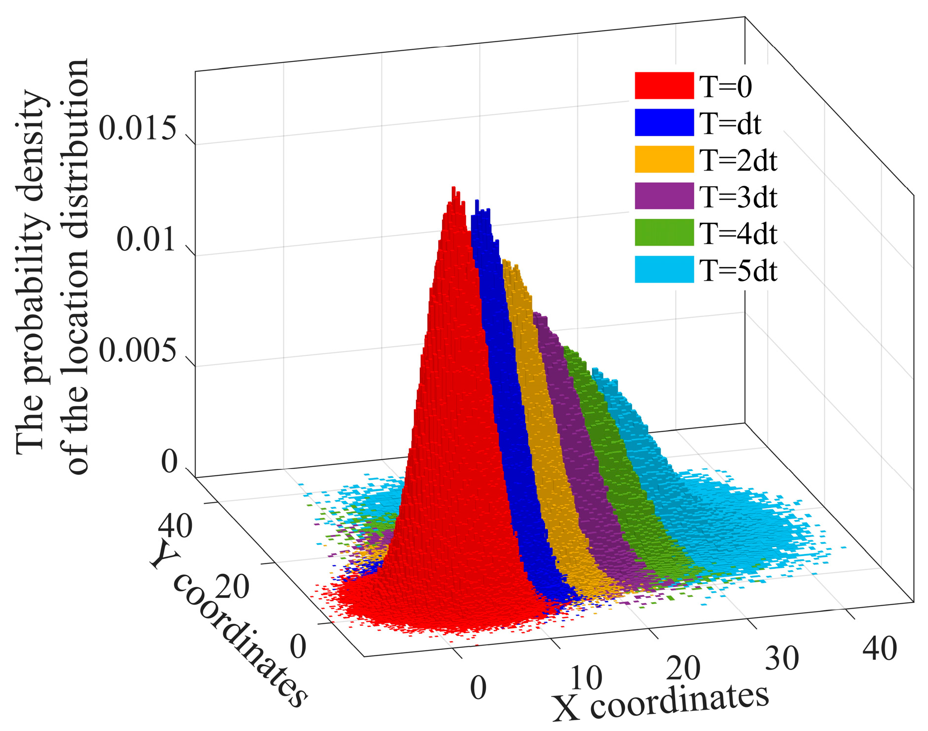
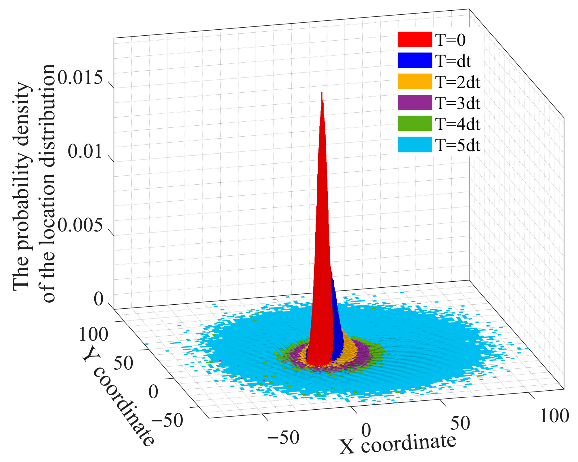
Under the same initial conditions, the GMMIM and the RPPM are, respectively, used to estimate the probability density of the target position distribution at time T = d t , 2 d t , 3 d t , 4 d t , 5 d t , as shown in Figure 2 and Figure 3. The Z-coordinate represents the probability density value of the target appearing at a certain point ( x , y ) .
Figure 2 shows that the target position distribution estimated by GMMIM presents a pattern of “gradual diffusion with local concentration”. The central high-density area reflects the model’s “memory” of the target’s historical states, while the surrounding scattered points expand adaptively over time. This aligns with the characteristics of the Gaussian–Markov process, which balances state continuity and environmental uncertainty. In contrast, the results of RPPM in Figure 3 show a “spiky” distribution of probability density at each moment. The narrow central peak indicates that RPPM directly propagates uncertainties based solely on initial statistical parameters, lacking the ability to adaptively adjust to dynamic state changes.
The above analysis shows that GMMIM can better capture the motion dynamics of targets in uncertain environments and generate “more smoothly evolving distributions” over time steps. This provides reasonable spatial position uncertainty boundaries for the large-scale search missions of UAV swarms.

2.2. Modeling of Cluster Task Scheduling Problems

In UAV swarm search tasks, the heterogeneity of target values, environmental uncertainties, and UAV coordination constraints are intertwined. Precise problem modeling is required to transform complex task requirements into a computable and optimizable mathematical framework. This section focuses on modeling cluster task scheduling problems and constructs a complete mathematical model from “task allocation logic” to “benefit–cost quantification”. By defining a task allocation matrix to clarify the association between UAVs and targets, and combining the target position probability distribution to establish quantitative expressions for task execution costs and benefits, it lays a theoretical foundation for subsequent algorithm design and simulation experimental analysis, achieving the transformation from “task requirements” to “mathematically solvable problems”.

2.2.1. Optimization of Task Allocation Logic

In the cluster search tasks of multiple UAVs for multiple targets, the assignment matrix intuitively demonstrates the task scheduling of each UAV assigned to each target in the form of a matrix [21]. The task assignment relationship between UAVs and targets is generally described using a discrete 0/1 assignment matrix A M × N = ( a i j ) M × N :
A M × N = a 11 a 12 a 1 N a 21 a 22 a 2 N a M 1 a M 2 a M N
where M is the number of UAVs performing search tasks, and N is the number of target units. If a i j = 1 , it indicates that UAV i is assigned to target j ; otherwise, a i j = 0 .
The elements of the above allocation matrix only take two discrete values, 0 and 1, clearly representing the binary relationship of whether a UAV is allocated to a target or not. Each UAV can either fully take on or completely not take on the search task of a certain target. The task allocation is rather rigid, with no intermediate states. In some simple scenarios where task allocation requirements are clear and there is no resource sharing or partial participation, a “0/1 allocation” scheme with good performance can be obtained by solving the integer non-convex optimization problem. However, this “hard allocation” scheme also has prominent problems such as inflexible task scheduling, inability to accurately reflect task priorities and differences in UAV capabilities, lack of dynamic adjustment capabilities for the task execution process, and a tendency to fall into local optimal solutions.
Therefore, this paper designs a continuous 0–1 assignment matrix B M × N = ( b i j ) M × N to reflect the task assignment relationship between UAVs and targets:
B M × N = b 11 b 12 b 1 N b 21 b 22 b 2 N b M 1 b M 2 b M N
where b i j ( 0 b i j 1 ) represents the task proportion or resource allocation coefficient for assigning UAV i to target j . It satisfies the constraint Σ j = 1 N b i j = 1 , i = 1 , 2 , , M , meaning the sum of task proportions for each UAV assigned to all targets is 1. In underactuated scenarios (where the number of task units is less than the number of targets), this continuous “soft allocation” scheme can dynamically respond to various uncertainties. It enables more refined resource and task allocation based on UAVs’ capabilities and targets’ priorities. By leveraging continuous space to avoid integer non-convex optimization issues, it effectively improves the cluster’s task scheduling efficiency.

2.2.2. Calculation of Task Execution Position

For each task unit, the expected position ( x ˜ i , y ˜ i ) for performing the search task can be determined according to the continuous allocation matrix B M × N and the probability density of the position distribution of the target unit. For the target unit j ( j = 1 , 2 , , N ) , its position probability density function is p j ( x , y ) . For the UAV i ( i = 1 , 2 , , M ) , its allocation weight vector to the targets is ω i = ( b i 1 , b i 2 , , b i N ) . Then, the expected position ( x ˜ i , y ˜ i ) for the UAV i to perform search tasks is expressed as:
x ˜ i = j = 1 N b i , j x p j ( x , y ) d x d y y ˜ i = j = 1 N b i , j y p j ( x , y ) d x d y

2.2.3. Modeling of Task Scheduling Cost

Due to the limited overall task time and the possible threat of targets, the scheduling cost needs to be taken into account when formulating the task scheduling strategy. This cost depends on the time required for the unit to reach the predetermined location. Assuming the initial position of each UAV at the start of the task is ( x i , 0 , y i , 0 ) , the task scheduling cost can be quantified as:
χ B , p ( t ) = i = 1 M ( x ˜ i , t x i , 0 ) 2 + ( y ˜ i , t y i , 0 ) 2
Among them, χ B , p ( t ) represents the task scheduling cost under the specific allocation matrix B M N and the target position probability distribution p t , and ( x ˜ i , t , y ˜ i , t ) represents the expected position of the i UAV to perform the search task at time t .

2.2.4. Modeling of Target Value Degree

The value degree c j of the j target unit depends on two aspects. First, the maneuver speed of the target unit, the degree of threat to task units, and the formation situation determine the basic value of the value degree. Second, the fuzziness of the information obtained by the pre-situational awareness module has a weighted impact on the value degree of the target unit. Assuming that the basic value of the value degree of the target unit with information credibility k j is c j * , then its final weighted value degree is represented as c j = k j c j * . The value degree matrix of each target in the task area is expressed as C = c 1 , c 2 , , c N . Under a specific allocation matrix B M × N , the target value benefit ϖ B of the search task is expressed as:
ϖ B = sum ( B M × N C ) = j = 1 N i = 1 M b i j c j

2.2.5. Quantitative Assessment of Task Execution Benefits

Under a certain task allocation scheme, the execution benefit of a search task depends on the target value benefit ϖ B and the task scheduling cost χ B , p ( t ) . This study uses a logical function f ( x ) to analyze the value embodiment of task execution and cost suppression:
f ( χ B , p ( t ) , ϖ B ) = s 1 + s 2 1 + e s 3 + s 4 χ ( B , p ( t ) ) l 1 + l 2 1 + e l 3 + l 4 ϖ ( B )
Among them, s 1 s 4 and s 1 s 4 are parameters of the logical function. By assigning values to the parameters, the weights of the target value benefit ϖ B and the task scheduling cost χ B , p ( t ) on the task execution benefit can be adjusted.

2.3. Optimization of Cluster Task Scheduling Strategy Based on Improved Gray Wolf Algorithm

The core problem of multi-UAV collaborative search task scheduling for multiple targets is how to rationally allocate UAVs to each target, obtain the optimal task allocation matrix, and maximize task execution benefits. Due to the complexity of the task environment and the highly dynamic nature of multiple targets, traditional task scheduling methods often struggle to meet the requirements of real-time performance and optimality. As an intelligent optimization algorithm, the Grey Wolf Optimizer (GWO) provides a new approach to solving the multi-UAV swarm task scheduling problem, thanks to its strong global search capability and fast convergence characteristic [22]. First, this chapter explores the overall framework of the GWO. Then, it focuses on analyzing the impact of the decay law of the convergence factor on the performance of the GWO. Finally, it proposes the Grey Wolf Optimizer integrated with sliding window technology (FSW-GWO).

2.3.1. Overall Framework of the Gray Wolf Optimization Algorithm

The GWO algorithm takes inspiration from the hunting behavior of grey wolf packs. These packs have a strict hierarchical structure, primarily consisting of four levels: α, β, δ and γ. α wolves are the leaders of the pack and are in charge of deciding the hunting direction. β wolves assist α wolves in the decision-making process. δ wolves follow the commands of α and β wolves. γ wolves are just ordinary members of the group.
In the algorithm, each grey wolf represents a potential solution, namely a task scheduling strategy (corresponding to a specific task allocation matrix). The algorithm searches for the optimal task scheduling strategy by iteratively updating the positions of the grey wolves. During iteration, the current top three solutions are determined based on task execution benefits, corresponding to α, β, and δ wolves, respectively. The remaining γ wolves update their positions according to the positional information of α, β, and δ wolves to gradually approach the optimal solution [23]. The overall framework of the algorithm is shown in Figure 4.
The optimization of the grey wolf algorithm for task scheduling of multi-target search by UAV swarm mainly consists of the following steps:
Step 1: Parameter initialization: Set the number of grey wolf individuals involved in the search as N G W , the maximum number of iterations as T , and the boundaries of the search space as B M × N = ( b i j ) M × N , b i j [ 0 , 1 ] .
Step 2: Population Initialization: Randomly generate N G W grey wolf individuals, each with M × N dimensions, where each individual represents a task allocation strategy.
Step 3: Fitness Value Calculation: For each task allocation strategy represented by a grey wolf individual, calculate its corresponding task execution benefit, i.e., the fitness value of the individual, based on the established quantitative models for task scheduling cost and execution benefit.
Step 4: Identify the α, β, and δ Wolves: Sort the individuals in the population based on their calculated fitness values. The individual with the highest fitness value is designated as the α wolf, representing the current optimal task scheduling strategy; the next highest is the β wolf; and the third highest is the δ wolf.
Step 5: Iterative Update: In each iteration, update the positions of other γ wolves based on the position information of the α, β, and δ wolves. The update formula is based on the simulation of grey wolf hunting behavior. It determines the new position by calculating the distance between the current individual and the α, β, and δ wolves, and combining it with a random coefficient vector. Then, recalculate the fitness values of the updated individuals and update the α, β, and δ wolves. The updated formulas are as follows:
D α = C 1 · X α X ( t ) , D β = C 2 · X β X ( t ) , D δ = C 3 · X δ X ( t ) X 1 = X α A 1 · D α , X 2 = X β A 2 · D β , X 3 = X δ A 3 · D δ X ( t + 1 ) = ( X 1 + X 2 + X 3 ) / 3
Among them, X ( t ) denotes the current grey wolf individual, which corresponds to the vectorized representation of the task assignment matrix; X α , X β , X δ represent the positions of α , β , δ wolves, respectively; A i , C i are coefficient vectors, with A i = λ ( 2 r i 1 1 ) , C i = 2 r i 2 in each iteration. r 1 , r 2 are random vectors within [0, 1], which are intended to increase search randomness and help the algorithm escape local optima. λ is the convergence factor, which decays from its maximum value to 0 during the iteration process. Its role is to control the convergence speed of the optimization algorithm and ensure a balance between the algorithm’s global search and local exploitation.
Step 6: Feasible Region Projection To ensure that the solutions generated during the iteration process always satisfy the constraint conditions of the task assignment matrix—i.e., after each position update, each assignment coefficient b i j is constrained to the range [0, 1] and the sum of elements in each row (of the matrix) equals 1—this study introduces a projection operation into the iterative update step of the Grey Wolf Optimizer. First, clip each updated b i j by setting b i j = max ( 0 , min ( 1 , b i j ) ) . Second, perform normalization on each row of the task assignment matrix to ensure the sum of elements in each row equals 1.
Step 7: Result Output: When the optimization algorithm reaches the maximum number of iterations T , output the task allocation strategy represented by the current optimal α wolf, i.e., the optimal cluster task scheduling scheme.

2.3.2. Decay Law of Convergence Factor

In the GWO, the convergence factor λ is a critical parameter for balancing the algorithm’s global exploration and local exploitation capabilities [24]. In the early stage of the algorithm, strong global search capability is required to explore potential optimal solution regions in a large search space. At this time, λ should be large, allowing grey wolf individuals to have a large search step size. As the iterations progress and the algorithm gradually approaches the optimal solution, it is necessary to enhance the local exploitation capability for fine-grained searching in the currently identified superior regions. In this case, λ should gradually decrease to reduce the search step size.
Common decay laws can be broadly divided into two categories: linear decay and non-linear decay. Under the linear decay law, the convergence factor λ decreases uniformly with the number of iterations, with a constant rate of change. The mathematical expression is λ t = λ 0 ( 1 t / T ) , where λ t represents the value of the convergence factor at the t-th iteration, and λ 0 represents the initial value of the convergence factor. The linear decay law is simple in principle and easy to implement. However, when facing complex problems, it struggles to accurately balance global and local search, which may lead to premature convergence and make it prone to falling into local optima in high-dimensional or multi-peak problems.
Under the non-linear decay law, the decay rate of the convergence factor changes with independent variables such as the number of iterations. Common non-linear decay laws include exponential decay [24], logarithmic decay, and piecewise function decay. The mathematical expression of exponential decay is:
λ t = λ 0 λ 0 ( e t / T 1 e 1 ) k
Its decay rate is denoted as η e . The mathematical expression of logarithmic decay is:
λ t = λ 0 λ 0 k log ( 1 + t ) log ( 1 + T )
Its decay rate is denoted as η log . k is a non-linear adjustment coefficient that determines the decay rate. Piecewise function decay divides the iteration process into different stages, with each stage using a different functional form to determine the value of the convergence factor. Compared to linear decay, nonlinear decay laws can flexibly balance global and local search. However, setting their nonlinear parameters reasonably often relies on prior knowledge of specific problems and repeated debugging, making it difficult to ensure stable and efficient convergence across all optimization scenarios.

2.3.3. Adaptive Dynamic Update Mechanism for Decay Rate Integrated with Sliding Window Technology

Sliding window is a technique for managing and processing data streams [25,26]. It enables efficient data processing, transmission control, and resource management by dynamically monitoring and analyzing population information during the algorithm’s search process. By defining a sliding window, it observes the fitness information within the window in each iteration to evaluate the current population’s search status. Therefore, this study introduces sliding window technology to design an adaptive dynamic update mechanism for the decay rate of the convergence factor. This mechanism automatically adjusts the decay rate based on the convergence degree of the population within the sliding window, thereby achieving a better search balance at different stages of the algorithm. Its implementation mainly consists of the following steps:
Step 1: Window definition and information collection. Select the sliding window length L based on prior knowledge such as the problem scale. In each iteration, collect and organize statistical information about the population’s optimal fitness f g b e s t within the current iteration and several previous iterations to comprehensively evaluate population diversity and convergence trends.
Step 2: Convergence degree evaluation. Select the standard deviation σ of the optimal fitness f g b e s t within the window as the population convergence degree indicator. A smaller σ indicates that the population’s optimal fitness values are relatively concentrated, and the population tends to converge; a larger σ means the population has high diversity and has not converged yet. Evaluate the convergence degree based on the information collected within the sliding window.
Step 3: Dynamically adjust the decay rate of the convergence factor according to the evaluated population convergence degree. The mathematical expression of the adaptive dynamic update mechanism is:
λ t + 1 = λ 0 exp [ ( k k σ t 4 σ 0 ) t 2 T 2 ]
Among them, k is the rate control parameter, a t + 1 represents the value of the convergence factor at the t + 1 iteration, σ t denotes the standard deviation of the population’s optimal fitness f i , g b e s t ( i [ t L / 2 , t + L / 2 ] ) within the sliding window after the t iteration, and σ 0 represents the standard deviation of the population’s optimal fitness f i , g b e s t ( i [ 1 , L ] ) at the 0 ~ L iterations, expressed as:
σ 0 = t = 1 L ( f i , g b e s t ( t = 1 L f i , g b e s t ) / L ) 2 / L
Taking the logarithmic decay rate η log as a reference, the above decay strategy of the convergence factor adaptively adjusts the decay speed of the convergence factor to dynamically change within [ 0.75 η e , η e ] by real-time evaluating the standard deviation of the population’s optimal fitness f g b e s t in the sliding window. When the population diversity is high and no obvious convergence occurs, the decay speed of the convergence factor is accelerated to urge the algorithm to narrow the search range faster and approach the optimal solution. Conversely, when the population tends to converge (i.e., the standard deviation of the optimal fitness in previous iterations is small), the decay speed of the convergence factor is slowed down to avoid the algorithm falling into local optima prematurely. This enables the algorithm to maintain a certain degree of global search capability and continue exploring a broader solution space.

3. Results and Discussion

To systematically verify the effectiveness of the UAV swarm task scheduling strategy optimization under uncertain information, this section first constructs a task scenario of multi-UAV cooperative search for multiple targets, and conducts estimation and verification of the targets’ real-time positions. Regarding the high-dimensional and multi-modal characteristics of the task scheduling problem, this section discusses the variation in the population’s optimal fitness with the iteration process under the application of different algorithms. Finally, it visually demonstrates the swarm task scheduling process.

3.1. Experimental Parameter Setting

The search mission is set as follows: Six task units (i.e., UAVs) depart from their initial positions (the origin) to conduct collaborative search operations on eight target units. The pre-situational awareness module integrates multi-peak perception and mission scenarios to acquire situational information such as the motion trajectories, speeds and accelerations, steering and attitude angle data of each target unit. Based on information such as the threat level, maneuvering speed, and role differentiation of the targets, the value level of each target unit is preliminarily determined. The value distribution reflects the non-uniformity of target priorities and simulates the differential characteristics of target importance in real scenarios. The initial position information and value levels of each target unit are assumed to be as shown in Table 1.
Among them, μ x 0 , μ y 0 are, respectively, the means of the coordinates of each target unit at the initial moment; μ V is the mean of the speed magnitudes of each target unit; μ θ is the mean of the speed directions of each target unit; c i is the value coefficient of each target unit. In addition, the relevant parameters of the improved grey wolf optimization algorithm are summarized in Table 2.
Among them, the logistic function is used to quantify the task execution benefit; its value is set to 1, which helps the experiment focus on the improvement of task scheduling efficiency by the improved grey wolf algorithm, rather than the weight adjustment of the benefit function itself. The population consists of 50 grey wolf individuals, which balances solution space coverage and computational complexity. The maximum number of iterations is set to 10,000 to ensure that the high-dimensional multi-modal optimization problem converges to the global optimum, while balancing experimental accuracy and feasibility. The sliding window length is set to 10, allowing for reasonable dynamic evaluation of the population’s convergence degree and matching the maximum number of iterations. The adjustment parameter for the decay rate is set to 5, which is based on robustness verification in pre-experiments, ensuring a smooth transition of the convergence factor between global search and local exploitation.
Based on the above initial situation and parameter presetting of the grey wolf optimization algorithm, four types of core experiment verification analyses are sequentially carried out in the follow-up. First, the Gaussian–Markov Memory Iteration Method (GMMIM) is applied to explore the evolution law of the position distribution of target units under uncertain information. Meanwhile, an ablation experiment is designed to verify the effectiveness of the “target position estimation” module (when applying the GMMIM) in improving the task scheduling efficiency of UAV swarms in the scenario of maritime target search. Second, simulation of the high-dimensional multi-peak characteristics of the task scheduling optimization problem is conducted. The t-distributed Stochastic Neighbor Embedding (t-SNE) method is employed to perform dimensionality reduction mapping on the task allocation matrix, visualizing the multi-peak structure of the strategy space. Third, simulation of the change in the population’s optimal fitness with the iteration process is carried out to track the convergence trend of fitness during algorithm iteration and verify the optimization efficiency of the scheduling strategy. Fourth, visual simulation of cluster task scheduling is conducted to intuitively present the task allocation and collaborative search process of the UAV swarm. Through multi-dimensional verification analysis, the performance of the proposed task scheduling strategy in multi-target search tasks is comprehensively tested.

3.2. Target Position Estimation and Verification

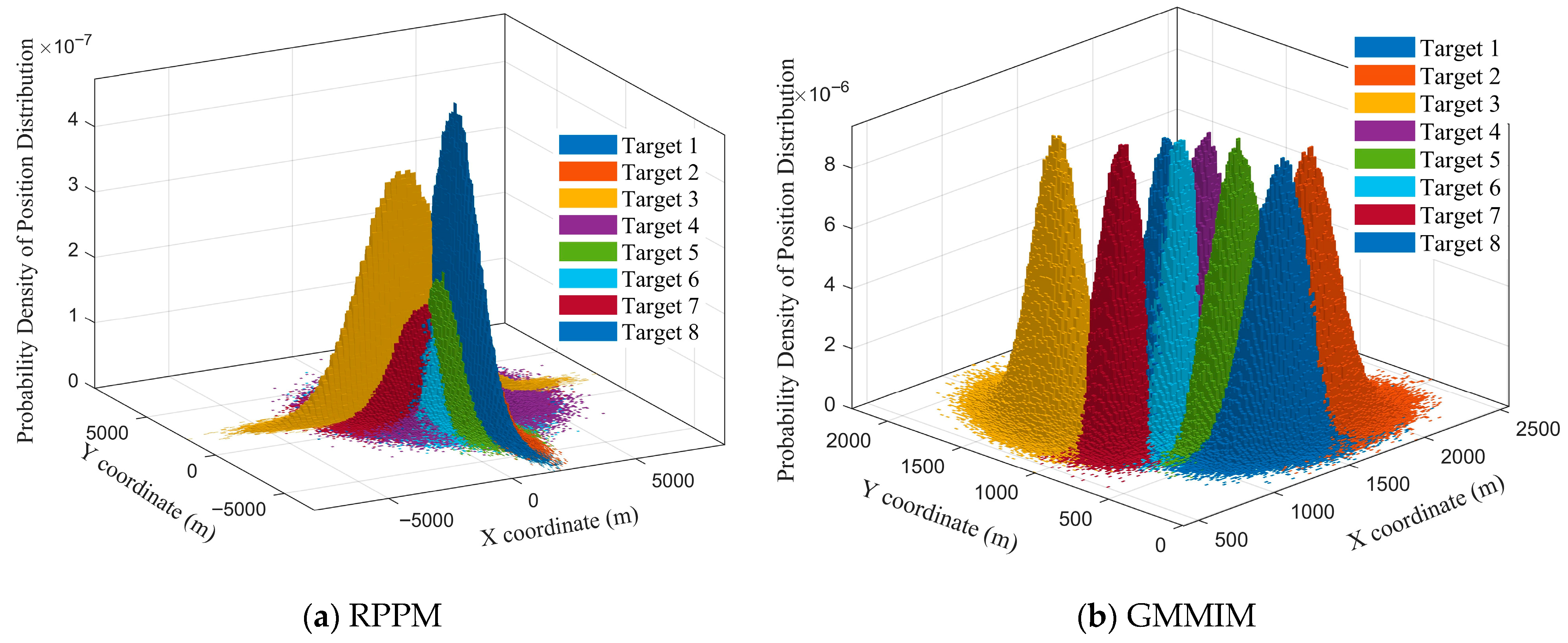
The analysis in Section 2.1.3 shows that compared with the RPPM, when the GMMIM is applied to estimate the target position distribution, it generates “more smoothly evolving distributions” over time steps, which provides reasonable and limited spatial range uncertainty boundaries for the search tasks of UAV swarms. Therefore, this section uses RPPM and GMMIM, respectively, to estimate the probability density of the position distribution of 8 target units (Target 1–8) under the initial scenario, and the results are shown in Figure 5. Different color clusters correspond to the position distributions of different units.
Figure 5 reveals that under the RPPM, the position distributions of some targets exhibit narrow-range spike-like patterns, whereas those of the remaining targets are relatively scattered and sparse. In contrast, under the GMMIM, the distributions of all targets demonstrate spatial distinguishability and local concentration, indicating that the model effectively captures differences in motion characteristics between targets and achieves decoupled estimation of multi-target distributions. The dense point traces within the same color cluster reflect the “memory property” of GMMIM regarding the target’s historical states, which confirms that GMMIM, through a serial iteration mechanism, integrates the state continuity constraints of the Gaussian–Markov process and the capability of uncertainty modeling.
Next, an ablation experiment is designed to verify the effectiveness of the “target position estimation” module (under the GMMIM) in improving the task scheduling efficiency of UAV swarms in the scenario of maritime target search. The baseline control group uses the GMMIM to estimate target positions (as shown in Figure 5b), while the ablation experimental group adopts the RPPM for target position estimation (as shown in Figure 5a). Using the FSW-GWO method designed in this study, the task execution positions of the search units are calculated, with the statistics presented in Table 3.
The comparative experiments show that the search units in the baseline control group and the ablation experimental group have significant differences in their task execution positions. Compared with the baseline control group, the population’s optimal fitness of the ablation experimental group decreases by 5.36%. Assuming that the reliable search distance of the search units is 300 m, Figure 6 compares the probability of successfully capturing targets between the two groups of simulation experiments.
Figure 6 shows that under the application of RPPM, the task scheduling efficiency of the UAV swarm decreases significantly: the probability of successfully capturing Targets 1, 3, 4, 7, and 8 drops by 56.42% to 61.03%; the probability of successfully capturing Targets 5 and 6 is basically the same as that of the baseline control group; and the probability of successfully capturing Target 2 decreases slightly. The above analysis shows that GMMIM reliably estimates the positional probability distributions of each target, providing reasonable spatial distribution uncertainty and high-resolution, differentiated target situation support for the subsequent “UAV-target” matching optimization in swarm task scheduling.

3.3. High-Dimensional Multi-Peak Characteristics of the Task Scheduling Optimization Problem

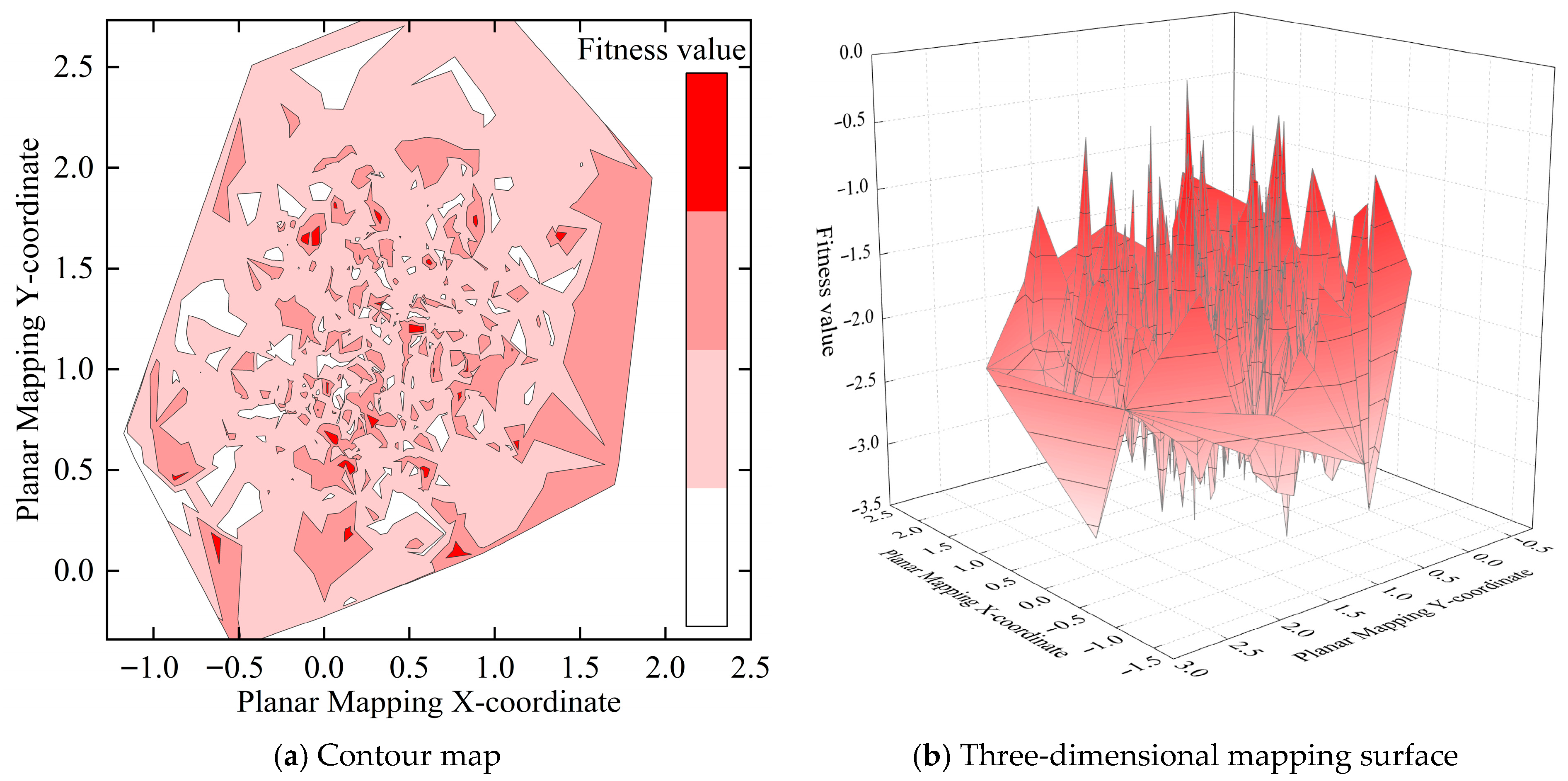
The t-distributed Stochastic Neighbor Embedding (t-SNE) method is a nonlinear dimensionality reduction technique based on a probabilistic model that maps high-dimensional data into two- or three-dimensional space to visualize data distributions and reveal the intrinsic structure and similarities within the data [27,28]. To characterize the high-dimensional multi-peak characteristics of the optimization problem in cluster task scheduling strategies, this paper employs the t-SNE method to map the high-dimensional data of the task allocation matrix into a two-dimensional space for analysis, as shown in Figure 7.
Figure 7a presents the strategy distribution in a planar mapping form. The horizontal and vertical coordinates correspond to the two-dimensional traces after t-SNE dimensionality reduction, while the color gradient reflects the magnitude of task execution benefits. Notably, the high-benefit regions indicated by red exhibit discrete and multi-peak distributions, surrounded by low-benefit regions in light and white colors. This visually demonstrates the high-dimensional multi-peak characteristics of the strategy space, where “high-quality solutions are dispersed and local optimal solutions are numerous.” Figure 7b further quantifies the benefit distribution in the form of a three-dimensional surface. The X and Y axes continue the two-dimensional trace mapping, while drastic fluctuations in fitness values shown on the Z axis clearly reveal the multi-peak morphology of this optimization problem. Sharp and staggered peaks correspond to high-benefit strategy clusters, while troughs represent inefficient allocation schemes.
Taken together, the two figures indicate that the strategy space for cluster task scheduling contains numerous local optimal structures, with high-quality scheduling patterns being dispersed and isolated from each other—validating the problem’s high-dimensional multi-peak nature. Meanwhile, this visualization inspires that subsequent algorithm design must break through the “peak trap” of local optima and establish cross-regional search mechanisms to uncover globally superior task allocation strategies.

3.4. Changes in Population Optimal Fitness During the Iteration Process

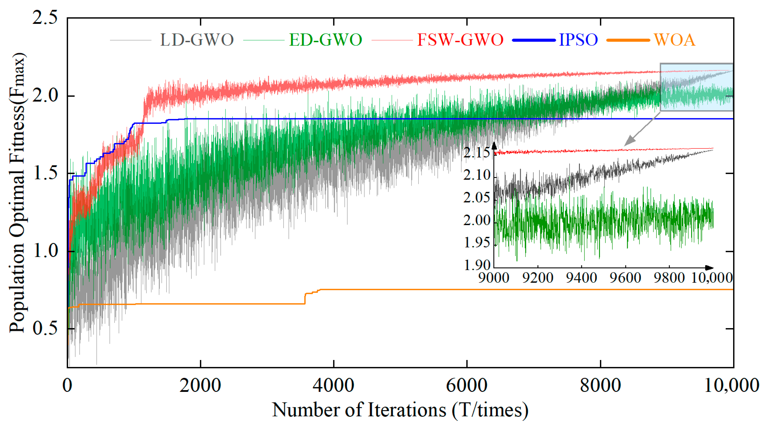
The analysis in Section 3.3 shows that the task scheduling of UAV swarms for multi-target search is a typical “high-dimensional multi-modal” optimization problem, and an optimization algorithm with a cross-regional search mechanism should be designed. Section 2.3.2 points out that the convergence factor is a key parameter for balancing the global search and local exploitation capabilities of the algorithm. Based on integrating sliding window technology, a dynamic adaptive update mechanism for the decay rate of the convergence factor is designed. Therefore, this section studies the variation in the population’s optimal fitness with the iteration process under three different strategies: linear decay, exponential decay, and dynamic adaptive decay. These strategies correspond to the three result curves (LD-GWO, ED-GWO, and FSW-GWO) in Figure 8, respectively. In addition, this section also compares the performance of FSW-GWO in solving high-dimensional multi-modal problems with that of popular algorithms, such as the Improved Particle Swarm Optimization (IPSO) [29] and the Whale Optimization Algorithm (WOA) [30]. Table 4 and Table 5 present the key parameters of IPSO and WOA, respectively.
To ensure the objectivity and credibility of the comparative experiments, the number of particles, maximum number of iterations, and problem dimension of IPSO are kept consistent with those of the improved gray wolf optimization algorithm (GWO) adopted in this study. As one of the core parameters of IPSO, the initial inertia weight controls the degree to which particles inherit their historical velocity. The initial value of the initial inertia weight is set to 0.9 and decreases linearly to 0.4 with iterations, which balances the algorithm’s global exploration capability in the early stage and local exploitation capability in the later stage. The cognitive factor and social factor of IPSO are both set to 0.5, ensuring that particles retain a portion of their individual experience and balance the use of group information and individual information.
To ensure the objectivity and credibility of the comparative experiments, the Population Size, Maximum Number of Iterations, and Problem Scale of WOA (Whale Optimization Algorithm) are kept consistent with those of the improved gray wolf optimization algorithm (GWO) adopted in this study. The encircling coefficient A determines the algorithm’s search strategy: when A < 1 , the algorithm implements the shrinking encircling mechanism and approaches the current optimal solution; when A 1 , it executes the random search mechanism and moves toward a randomly selected individual. The weight coefficient is a random number within the range [0, 2), which is not affected by the number of iterations and maintains randomness consistently to prevent the algorithm from premature convergence. The spiral shape coefficient is usually set to 1 to ensure the stability of the spiral shape. The spiral angle coefficient varies within [−1, 1] during the iteration process, which enhances the diversity of spiral search.
Simulation results show that under the application of different algorithms, the population’s optimal fitness gradually increases with the iteration process. In the early iteration stage, the improvement rate of the population’s optimal fitness for FSW-GWO and IPSO is significantly higher than those for the other three algorithms. This indicates that these two algorithms have stronger global exploration capabilities in the initial stage and can capture high-quality solutions more efficiently. In the late stage of iteration: the optimization result of ED-GWO fluctuates violently around 2; the optimization result of LD-GWO reaches 2.162; the optimization result of IPSO stabilizes at 1.852; the convergence value of WOA’s optimization result is only 0.753; while FSW-GWO, on the basis of ensuring stable convergence, achieves an optimization result of 2.166, which is 2.12% and 16.95% higher than that of LD-GWO and IPSO, respectively.
Simulation results show that for the gray wolf optimization algorithm (GWO) under fixed decay modes such as ED-GWO and LD-GWO, there are issues of slow fitness improvement in the early stage and insufficient convergence accuracy in the later stage. These variants cannot dynamically adjust the decay rate of the convergence factor according to the actual growth of the population’s optimal fitness, making it difficult to achieve an effective balance between global exploration and local exploitation. Due to insufficient diversity in its spiral update and encircling mechanisms, WOA (Whale Optimization Algorithm) is prone to falling into local optima in the early stage of iteration. Its global exploration capability is limited, making it hard to traverse the high-dimensional multi-modal solution space. IPSO (Improved Particle Swarm Optimization) relies on an update mechanism based on individual and group information sharing. It is easy for some particles to fall into local optima, which triggers “premature convergence” of the population. Even with improvements, if the parameter adaptability is insufficient, it still cannot fully explore the multi-modal solution space. In high-dimensional multi-modal optimization problems, both algorithms (WOA and IPSO) exhibit poor convergence accuracy and global optimization performance due to the lack of either global exploration capability or the ability to resist local optima. In contrast, the dynamic adaptive decay rule provides a more efficient dynamic adaptive parameter adjustment strategy for GWO by flexibly adjusting the convergence factor when addressing large-scale high-dimensional multi-modal problems such as swarm task scheduling strategy optimization.

3.5. Visualization of Cluster Task Scheduling

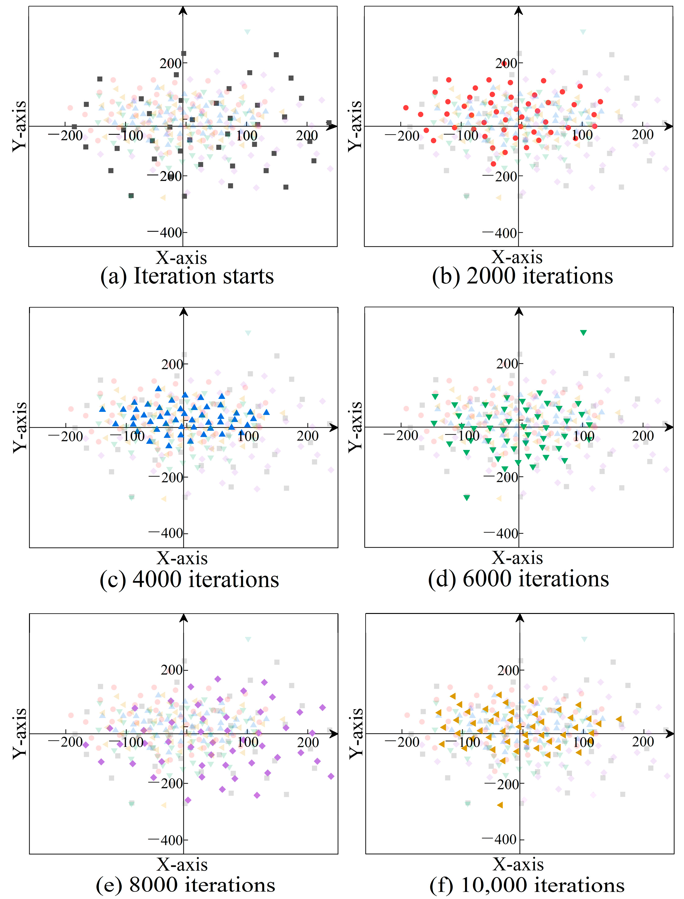
To visualize the optimization process of cluster task scheduling, this section uses the t-SNE method to map the high-dimensional matrix represented by each gray wolf in the population into a two-dimensional space. The t-SNE method ensures that the convergence and divergence of the gray wolf population are consistent with those of the point traces in the two-dimensional space. Figure 9 shows the changes in the two-dimensional point traces of the gray wolf population at different iteration stages, realizing the low-dimensional representation of high-dimensional optimization.
Figure 9 shows that in the initial stage (Figure 9a), grey wolf individuals in the population are widely dispersed, reflecting the algorithm’s extensive exploration capability of the solution space. As the number of iterations increases (Figure 9b–f), individuals gradually converge toward certain core areas, indicating that the algorithm can effectively guide the population to converge toward potential optimal solution regions and exhibits good convergence characteristics. Notably, during the iteration process, the population does not remain confined to a single region but instead demonstrates exploration and aggregation across multiple regions at different stages. This suggests that the algorithm balances “global exploration” and “local exploitation” by dynamically adjusting the decay rate of the convergence factor, enabling it to escape local optima to some extent. Collectively, these characteristics demonstrate the effectiveness of the improved grey wolf algorithm in addressing high-dimensional multi-peak optimization problems such as multi-target search by UAV swarm.

4. Conclusions

4.1. Main Contributions

This paper focuses on UAV swarm search missions. Aiming at core challenges such as spatiotemporal uncertainty of target positions, high-dimensional multi-peak characteristics of task scheduling, and dynamic constraints of cluster coordination, it constructs a technical system of “situation awareness-strategy optimization-collaborative execution”. This system achieves precise calculation and dynamic adaptation of cluster task scheduling in uncertain environments.
(1). Considering the temporal correlation and spatial continuity of target movement, this study proposes a Serial Memory Iterative Method (GMMIM) integrated with the Gaussian–Markov mobility model, which improves task scheduling efficiency by 5.36%. Relying on the state transition mechanism of the Markov model, the method captures the correlations between the current state and historical states, dynamically depicts the evolutionary laws of multi-target position distribution, and effectively suppresses the cumulative errors of uncertain information. This provides high-confidence target situation support for task scheduling.
(2). To address the high-dimensional multi-modal optimization challenge of swarm task scheduling, this study updates the discrete 0/1 assignment matrix to a continuous 0–1 soft assignment scheme. Meanwhile, combined with the improved gray wolf optimization algorithm (GWO), it constructs an adaptive update mechanism for the convergence factor integrating sliding window technology. The designed FSW-GWO algorithm improves optimization performance by 16.95% compared with the IPSO method. This scheme dynamically adjusts task weights to adapt to the demand for flexible resource allocation in underactuated task scenarios. It breaks through the local optimum trap in high-dimensional multi-modal spaces and ensures efficient swarm task scheduling in dynamic environments.
(3). To address challenges posed by dynamic constraints in cluster coordination, this study uses dynamically updated task allocation weights to drive autonomous spatial coordination and complementarity in UAV swarm. Each search unit focuses on high-value targets while achieving global coverage through complementary distribution, based on target value heterogeneity and location distribution differences. The high coincidence between UAV positions and target location distribution in the final steady state verifies the scientific nature of the “situation awareness-strategy execution-effect verification” closed loop.
The “State Perception-Strategy Optimization-Coordinated Execution” UAV swarm task scheduling technology system proposed in this paper integrates the series memory iteration method based on the Gaussian–Markov model, the improved gray wolf optimization algorithm (GWO) with sliding window technology introduced, and the dynamic task weight update mechanism. This system can effectively cope with the interference of multi-source uncertain information in scenarios such as maritime search and rescue and disaster emergency response. It provides accurate target situation support and efficient scheduling strategies for UAV swarms, and improves their task execution efficiency and robustness in complex dynamic environments.

4.2. Research Limitations and Future Outlook

This study still has limitations in three aspects. First, the Gaussian–Markov Memory Iterative Method (GMMIM) used for target position estimation assumes that external environmental interference (e.g., air currents and electromagnetic noise) follows a stationary distribution. However, in real-world complex scenarios, sudden non-stationary interference can reduce the accuracy of position estimation. Second, the experimental scenarios focus on maritime multi-target search and do not cover multi-domain heterogeneous collaboration scenarios (air-land–sea). Additionally, the adaptability to capability differences between different types of UAVs (e.g., fixed-wing and rotary-wing UAVs) is insufficient. Third, when the improved gray wolf optimization algorithm (GWO) is applied to ultra-large-scale task scheduling (e.g., matching of hundreds of UAVs with dozens of targets), the computational complexity of sliding window data processing increases, which may affect the real-time scheduling performance.
Future research will focus on addressing the aforementioned limitations. First, to tackle non-stationary interference, an adaptive noise estimation module will be introduced to optimize the Gaussian–Markov model, thereby enhancing the robustness of position estimation in dynamic environments. Second, the research will expand scenarios to multi-domain collaboration, integrating multi-source sensing data from satellites, ground base stations, and other sources to establish a cross-platform task scheduling model. Finally, the algorithm architecture will be optimized: distributed computing will be integrated to reduce the complexity of ultra-large-scale tasks; meanwhile, the integration of reinforcement learning and intelligent optimization algorithms will be explored to further improve the adaptive scheduling capability in dynamic scenarios.

Author Contributions

Conceptualization, H.X.; Methodology, X.B. and Z.S.; Software, X.B. and H.X.; Validation, H.X., Z.S. and W.H.; Formal analysis, G.Z.; Investigation, Z.S. and G.Z.; Writing—original draft, X.B. and Z.S.; Writing—review & editing, G.Z.; Visualization, W.H.; Supervision, Z.S.; Project administration, W.H. All authors have read and agreed to the published version of the manuscript.

Funding

This research received no specific funding.

Data Availability Statement

Due to the involvement of commercial secrets, the data generated in this study can be obtained upon request from the corresponding author.

Acknowledgments

We sincerely thank the colleagues and teachers who contributed to this research.

Conflicts of Interest

The authors declare that there are no financial or non-financial interests, whether direct or indirect, that are related to the work submitted for publication. All contributions to this research are driven by academic exploration and the pursuit of scientific advancement, without any conflicts of interest arising from commercial, personal, or other interests that could influence the content or findings presented in this paper. In addition, regarding the use of generative artificial intelligence (AI) models in this manuscript, the declaration is as follows: During the preparation of the manuscript, generative AI models were mainly used to assist in the literature retrieval, draft the initial version of the introduction, help organize the logical flow of the text, and support the translation of the manuscript. It is important to note that no generative AI tools were used in the data processing, refinement of core innovations, or result analysis of this study. All content in the manuscript that was generated or co-generated with AI assistance has been fully reviewed, revised, and verified by the corresponding author and all co-authors to ensure the content is accurate, original, consistent with the study’s data and conclusions, and compliant with academic ethical standards. The authors bear full responsibility for the final content, completeness, and scientific validity of the manuscript.

Abbreviations

The following abbreviations are used in this manuscript:
RPPMRecursive probability propagation method
GMMIMGaussian–Markov memory iteration method
FSW-GWOThe Grey Wolf Optimizer integrated with sliding window technology

References

  1. Jiang, Z.; Sun, X.; Wang, W.; Zhou, S.; Li, Q.; Da, L. Path planning method for maritime dynamic target search based on improved GBNN. Complex Intell. Syst. 2025, 11, 296. [Google Scholar] [CrossRef]
  2. Tong, P.; Yang, X.; Yang, Y.; Liu, W.; Wu, P. Multi-UAV Collaborative Absolute Vision Positioning and Navigation: A Survey and Discussion. Drones 2023, 7, 261. [Google Scholar] [CrossRef]
  3. Li, J.; Zhang, G.; Jiang, C.; Zhang, W. A Survey of Maritime Unmanned Search System: Theory, Applications and Future Directions. Ocean Eng. 2023, 285, 115359. [Google Scholar] [CrossRef]
  4. Luo, J.; Dong, W. Accurate Positioning Method of Maritime Search and Rescue Target Based on Binocular Vision. Signal Image Video Process. 2025, 19, 311. [Google Scholar] [CrossRef]
  5. Ai, B.; Jia, M.; Xu, H.; Xu, J.; Wen, Z.; Li, B.; Zhang, D. Coverage Path Planning for Maritime Search and Rescue Using Reinforcement Learning. Ocean Eng. 2021, 241, 110098. [Google Scholar] [CrossRef]
  6. Wang, G.; Wei, F.; Jiang, Y.; Zhao, M.; Wang, K.; Qi, H. A Multi-AUV Maritime Target Search Method for Moving and Invisible Objects Based on Multi-Agent Deep Reinforcement Learning. Sensors 2022, 22, 8562. [Google Scholar] [CrossRef] [PubMed]
  7. Wen, H.; Shi, Y.; Wang, S.; Chen, T.; Di, P.; Yang, L. Route Planning for UAVs Maritime Search and Rescue Considering the Targets Moving Situation. Ocean Eng. 2024, 310, 118623. [Google Scholar] [CrossRef]
  8. Bays, M.J.; Wettergren, T.A.; Shin, J.; Chang, S.; Ferrari, S. Persistent Schedule Evaluation and Adaptive Re-Planning for Maritime Search Tasks. J. Intell. Robot. Syst. 2024, 110, 65. [Google Scholar] [CrossRef]
  9. Gungor, M. Classification and comparison of integer programming formulations for the single-machine sequencing problem. Comput. Oper. Res. 2025, 173, 106844. [Google Scholar] [CrossRef]
  10. Dias, F.; Rey, D. Aircraft Conflict Resolution with Trajectory Recovery Using Mixed-Integer Programming. J. Glob. Optim. 2024, 90, 1031–1067. [Google Scholar] [CrossRef]
  11. Clausen, J.V.; Crama, Y.; Lusby, R.; Rodriguez-Heck, E.; Ropke, S. Solving unconstrained binary polynomial programs with limited reach: Application to low autocorrelation binary sequences. Comput. Oper. Res. 2024, 165, 106586. [Google Scholar] [CrossRef]
  12. Zaccone, R. A Dynamic Programming Approach to the Collision Avoidance of Autonomous Ships. Mathematics 2024, 12, 1546. [Google Scholar] [CrossRef]
  13. Lin, A.; Liu, D.; Li, Z.; Hasanien, H.M.; Shi, Y. Heterogeneous differential evolution particle swarm optimization with local search. Complex Intell. Syst. 2023, 9, 6905–6925. [Google Scholar] [CrossRef]
  14. Zhou, X.; Li, R.; Wu, Z. Scheduling optimization for laminated door machining shop based on improved genetic algorithm. Comput. Oper. Res. 2025, 180, 107078. [Google Scholar] [CrossRef]
  15. Yao, P.; Duan, X.; Tang, J. An Improved Gray Wolf Optimization to Solve the Multi-Objective Tugboat Scheduling Problem. PLoS ONE 2024, 19, e0296966. [Google Scholar] [CrossRef] [PubMed]
  16. Tang, J.; Duan, H.; Lao, S. Swarm Intelligence Algorithms for Multiple Unmanned Aerial Vehicles Collaboration: A Comprehensive Review. Artif. Intell. Rev. 2023, 56, 4295–4327. [Google Scholar] [CrossRef]
  17. Makhadmeh, S.N.; Al-Betar, M.A.; Abu Doush, I.; Awadallah, M.A.; Kassaymeh, S.; Mirjalili, S.; Abu Zitar, R. Recent Advances in Grey Wolf Optimizer, Its Versions and Applications: Review. IEEE Access 2024, 12, 22991–23028. [Google Scholar] [CrossRef]
  18. Plummer, M. Simulation-Based Bayesian Analysis. Annu. Rev. Stat. Its Appl. 2023, 10, 401–425. [Google Scholar] [CrossRef]
  19. Baz, J.; Alonso, P.; Pena, J.M.; Perez-Fernandez, R. Gaussian Markov Random Fields over Graphs of Paths and High Relative Accuracy. J. Comput. Appl. Math. 2025, 453, 116142. [Google Scholar] [CrossRef]
  20. Kang, S.; Oh, H.-S. Novel Sampling Method for the von Mises-Fisher Distribution. Stat. Comput. 2024, 34, 106. [Google Scholar] [CrossRef]
  21. Luo, J.; Su, Y. Path Planning for Multi-USV Target Coverage in Complex Environments. Ocean Eng. 2024, 312, 119090. [Google Scholar] [CrossRef]
  22. Lu, Y.; Li, K.; Lin, R.; Wang, Y.; Han, H. Intelligent Layout Method of Ship Pipelines Based on an Improved Grey Wolf Optimization Algorithm. J. Mar. Sci. Eng. 2024, 12, 1971. [Google Scholar] [CrossRef]
  23. Qiu, Y.; Yang, X.; Chen, S. An Improved Gray Wolf Optimization Algorithm Solving to Functional Optimization and Engineering Design Problems. Sci. Rep. 2024, 14, 14190. [Google Scholar] [CrossRef] [PubMed]
  24. Arvaneh, F.; Zarafshan, F.; Karimi, A. Applying the Cheetah Algorithm to Optimize Resource Allocation in the Fog Computing Environment. Appl. Artif. Intell. 2024, 38, 2349982. [Google Scholar] [CrossRef]
  25. Nasir, M.; Sadollah, A.; Mirjalili, S.; Mansouri, S.A.; Safaraliev, M.; Jordehi, A.R. A Comprehensive Review on Applications of Grey Wolf Optimizer in Energy Systems. Arch. Comput. Methods Eng. 2025, 32, 2279–2319. [Google Scholar] [CrossRef]
  26. Papageorgiou, G.; Tjortjis, C. Adaptive Sliding Window Normalization. Inf. Syst. 2025, 129, 102515. [Google Scholar] [CrossRef]
  27. Allaoui, M.; Belhaouari, S.B.; Hedjam, R.; Bouanane, K.; Kherfi, M.L. T-SNE-PSO: Optimizing t-SNE Using Particle Swarm Optimization. Expert Syst. Appl. 2025, 269, 126398. [Google Scholar] [CrossRef]
  28. Neto, A.C.; Levada, A.L.M.; Haddad, M.F.C. Supervised t -SNE for Metric Learning With Stochastic and Geodesic Distances T-SNE Supervise Pour l’apprentissage Metrique Avec Des Distances Stochastiques et Geodesiques. IEEE Can. J. Electr. Comput. Eng. 2024, 47, 199–205. [Google Scholar] [CrossRef]
  29. Jain, M.; Saihjpal, V.; Singh, N.; Singh, S.B. An Overview of Variants and Advancements of PSO Algorithm. Appl. Sci. 2022, 12, 8392. [Google Scholar] [CrossRef]
  30. Makhadmeh, S.N.; Kassaymeh, S.; Rjoub, G.; Bataineh, B.; Sanjalawe, Y.; Al-Betar, M.A. Recent Advances in Multi-Objective Whale Optimization Algorithm, Its Versions and Applications. J. King Saud Univ. Comput. Inf. Sci. 2025, 37, 200. [Google Scholar] [CrossRef]
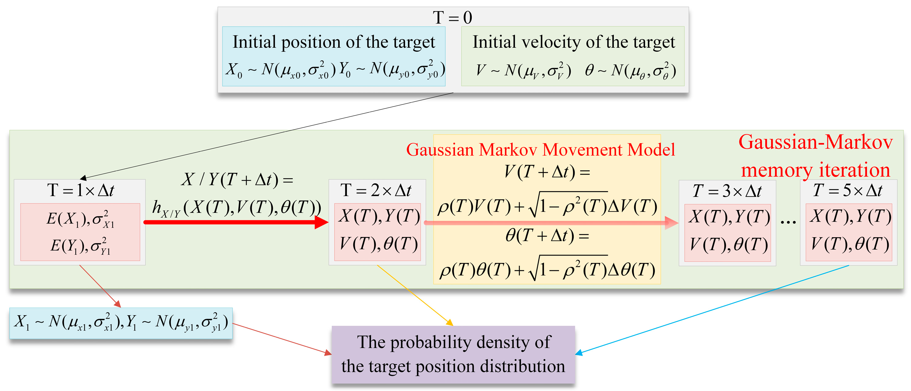
Figure 1. Principle of using GMMIM to obtain the real-time position distribution of the target.
Drones 09 00670 g001
Figure 2. Probability density of target position distribution under the application of GMMIM.
Drones 09 00670 g002
Figure 3. Probability density of target position distribution under the application of RPPM.
Drones 09 00670 g003
Figure 4. The overall framework of the Gray Wolf Optimizer algorithm.
Drones 09 00670 g004
Figure 5. Probability Density Estimation of Position Distributions for Each Target Unit Using Different Methods.
Drones 09 00670 g005
Figure 6. Statistics of the Probability of Successfully Capturing Targets.
Drones 09 00670 g006
Figure 7. High-Dimensional Multi-Peak Characteristics of the Optimization Problem for Cluster Task Scheduling Strategies.
Drones 09 00670 g007
Figure 8. The Variation in the Population’s Optimal Fitness with the Iteration Process Under the Application of Different Algorithms.
Drones 09 00670 g008
Figure 9. Visualization of the Optimization Process for Cluster Task Scheduling.
Drones 09 00670 g009
Table 1. Value Coefficients and Initial Positions of Each Target Unit.
Target T i ( μ x 0 , μ y 0 ) /m μ V /(kn) μ θ /rad c i
T 1 (500, 450)10.1791.2780.089
T 2 (500, 400)10.1981.4230.294
T 3 (500, 350)8.1210.2000.751
T 4 (500, 300)10.2121.4350.353
T 5 (450, 500)10.1780.9930.391
T 6 (400, 500)8.9640.1530.870
T 7 (350, 500)9.7740.4380.246
T 8 (300, 500)8.0810.8590.464
Table 2. Relevant Parameter Settings of the Grey Wolf Optimization Algorithm.
SymbolPhysical MeaningValue
s 1 ~ s 4 , l 1 ~ l 4 Parameters of the logical function1
N G W The number of grey wolf individuals in the population50
T Maximum number of iterations10,000
L The length of the sliding window10
k Adjustment parameter for the decay rate5
Table 3. Statistics of Task Execution Positions for Search Units.
Search UnitsBaseline Control GroupAblation Experimental Group
X-Coordinate/mX-Coordinate/mX-Coordinate/mX-Coordinate/m
Unit 11536.081098.531514.911474.49
Unit 21424.261228.001749.961288.57
Unit 31472.761137.961580.461373.33
Unit 41473.691092.041658.251267.78
Unit 51308.511230.561682.131121.60
Unit 61490.501000.481413.011302.29
Optimal Fitness2.1662.050
Table 4. Statistics of Key Parameters of IPSO.
Key ParametersParameter ValueParameter Meaning
Number of Particles50Controls population size and affects the algorithm’s search diversity
and computational efficiency; consistent with FSW-GWO
Maximum Number of Iterations10,000Affects convergence accuracy and convergence speed;
consistent with FSW-GWO
Problem Dimension6 × 8Determined by the task assignment matrix; consistent with FSW-GWO
Initial Inertia Weight0.9Controls the degree of the particle’s inheritance of its historical velocity
Final Inertia Weight0.4Linearly decreases to 0.4 with iterations,
enhancing the algorithm’s local exploitation capability in the later stage
Cognitive Factor1.5Controls the particle’s tendency to move toward its own historical optimal position
Social Factor1.5Controls the particle’s tendency to move toward the global optimal position
Table 5. Statistics of Key Parameters of WOA.
Key ParametersParameter ValueParameter Meaning
Population Size50Number of whale individuals; affects search diversity
and computational efficiency; consistent with FSW-GWO
Maximum Number of Iterations10,000Affects convergence accuracy and
convergence time; consistent with FSW-GWO
Problem Dimension6 × 8Determined by the task assignment matrix; consistent with FSW-GWO
Encircling Coefficientshrinks from [−2, 2] to [0, 0]Controls the algorithm’s switch between
random search strategy and shrinking encircling strategy
Weight Coefficient[0, 2)Introduces randomness to enhance the
algorithm’s ability to jump out of local optima
Spiral Shape Coefficient1Defines the spiral shape and intensity during spiral update; controls
the tightness of the spiral trajectory of individuals around the optimal solution
Spiral Angle Coefficient[−1, 1]Controls the angle during spiral update;
simulates the change in rotation angle of whales around prey
Disclaimer/Publisher’s Note: The statements, opinions and data contained in all publications are solely those of the individual author(s) and contributor(s) and not of MDPI and/or the editor(s). MDPI and/or the editor(s) disclaim responsibility for any injury to people or property resulting from any ideas, methods, instructions or products referred to in the content.