DFLM-YOLO: A Lightweight YOLO Model with Multiscale Feature Fusion Capabilities for Open Water Aerial Imagery

Abstract

Object detection algorithms for open water aerial images present challenges such as small object size, unsatisfactory detection accuracy, numerous network parameters, and enormous computational demands. Current detection algorithms struggle to meet the accuracy and speed requirements while being deployable on small mobile devices. This paper proposes DFLM-YOLO, a lightweight small-object detection network based on the YOLOv8 algorithm with multiscale feature fusion. Firstly, to solve the class imbalance problem of the SeaDroneSee dataset, we propose a data augmentation algorithm called Small Object Multiplication (SOM). SOM enhances dataset balance by increasing the number of objects in specific categories, thereby improving model accuracy and generalization capabilities. Secondly, we optimize the backbone network structure by implementing Depthwise Separable Convolution (DSConv) and the newly designed FasterBlock-CGLU-C2f (FC-C2f), which reduces the model’s parameters and inference time. Finally, we design the Lightweight Multiscale Feature Fusion Network (LMFN) to address the challenges of multiscale variations by gradually fusing the four feature layers extracted from the backbone network in three stages. In addition, LMFN incorporates the Dilated Re-param Block structure to increase the effective receptive field and improve the model’s classification ability and detection accuracy. The experimental results on the SeaDroneSee dataset indicate that DFLM-YOLO improves the mean average precision (mAP) by 12.4% compared to the original YOLOv8s, while reducing parameters by 67.2%. This achievement provides a new solution for Unmanned Aerial Vehicles (UAVs) to conduct object detection missions in open water efficiently.

1. Introduction

Object detection in open waters is crucial for maritime navigation, rescue operations, marine environmental monitoring, and national defense, with the primary goal of quickly identifying objects [1]. However, traditional search methods mainly rely on surface vessels and helicopters, which are inefficient and have limited range, making it difficult to accurately and quickly locate objects. Drones, due to their high mobility, low cost, and wide field of view, are widely used in agriculture, wildfire prevention, and disaster relief [2,3,4,5]. By integrating deep learning-based object detection algorithms, drones can autonomously detect objects, enhancing rescue efficiency [6].

The COCO dataset defines objects with a resolution smaller than 32 × 32 pixels as small objects [7]. In drone-based sea rescue missions, objects in aerial images are generally small due to the considerable distance from the sea surface and are affected by complex environments and varying scales, leading to poor detection performance. Limited onboard computational resources further challenge these algorithms. Therefore, object detection algorithms for open-water environments must meet real-time requirements with low parameter and computational costs while ensuring detection accuracy for small objects.

Current mainstream object detection algorithms are divided into single-stage and two-stage methods [8,9]. Two-stage algorithms, such as the R-CNN series, offer high detection accuracy but generate a large number of candidate boxes during detection, leading to high computational costs and slow detection speeds, making them unsuitable for applications requiring high real-time performance. To improve detection speed, Redmon et al. introduced the single-stage YOLO algorithm in 2015 [10]. Over the following years, researchers developed subsequent versions from YOLOv2 to YOLOv10 [11,12,13,14,15,16,17,18,19], with continuous improvements based on these models. The YOLO series features fast inference speeds, short training times, strong real-time performance, and fewer parameters, with detection accuracy continually improving. As a result, YOLO has become one of the most popular algorithms in object detection. Given the demands for computational resources, detection accuracy, and real-time performance in drone-based open-water search and rescue missions, this paper selects YOLOv8s as the baseline model.

To address the challenges encountered in open water search and rescue missions, this paper proposes a new lightweight multiscale feature fusion network, DFLM-YOLO. This network reduces model parameters and increases detection speed while enhancing the detection accuracy for small objects. Compared to the YOLOv8s, the improved model’s mAP50 increased by 12.4%, the model parameters decreased from 11.17 million to 3.65 million (a 67.3% reduction), the Floating Point of Operations (FLOPs) decreased from 28.7 to 23.3 (an 18.8% reduction), and the detection time decreased from 2.6 ms to 2.3 ms (an 11.5% reduction). This model outperforms other advanced small object detection algorithms in both speed and accuracy. The main contributions of this paper are as follows:

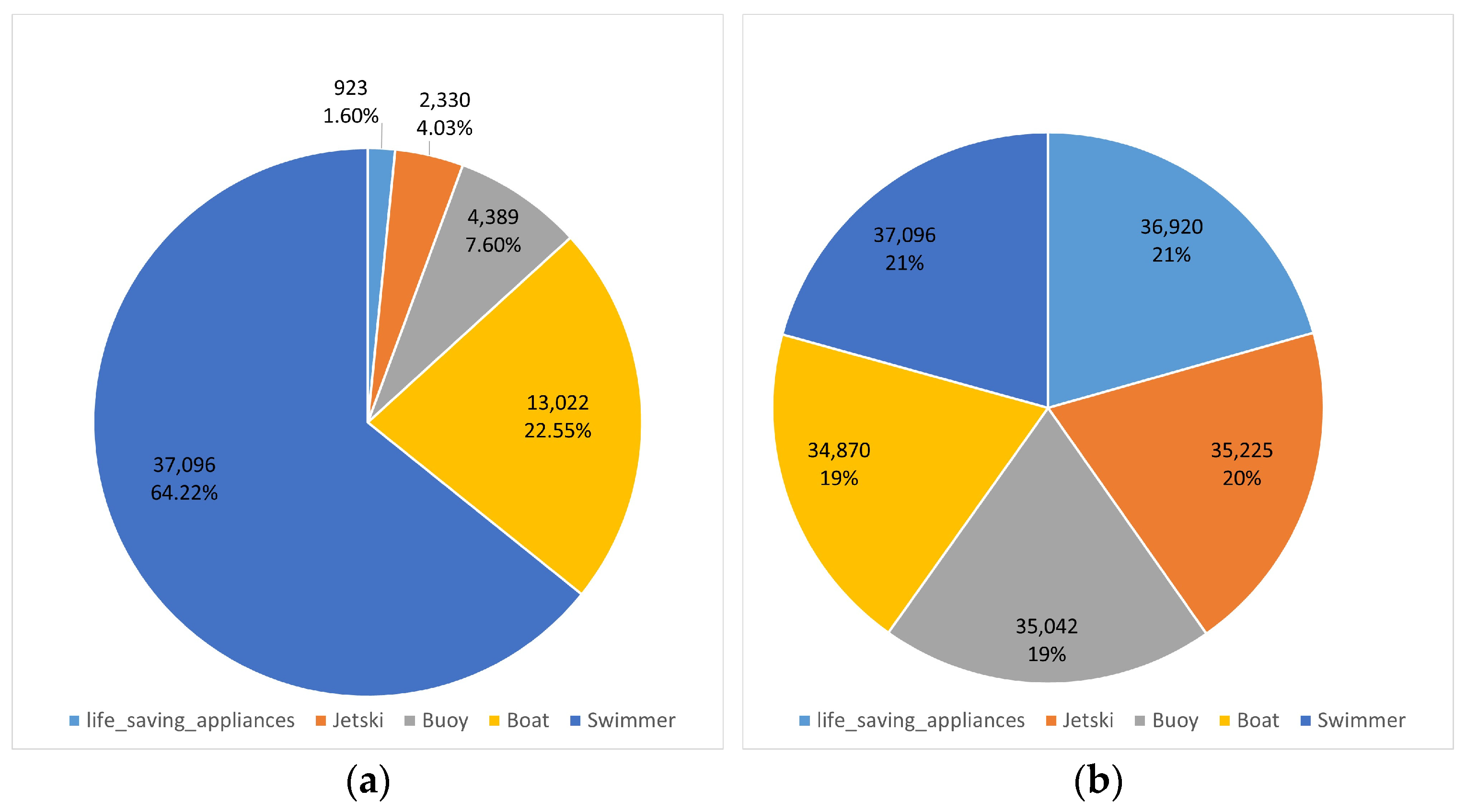
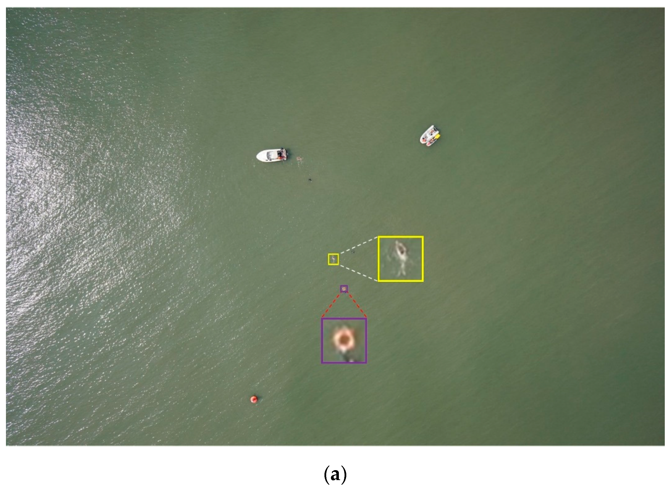
• The paper introduces a new data augmentation algorithm called SOM, which aims to expand the number of objects in specific categories without adding actual objects. This algorithm ensures that the characteristics of the added objects remain consistent with the original ones. The experiments demonstrate that this method enhances dataset balance and improves the model’s accuracy and generalization capabilities.
• A lightweight design of the backbone network:
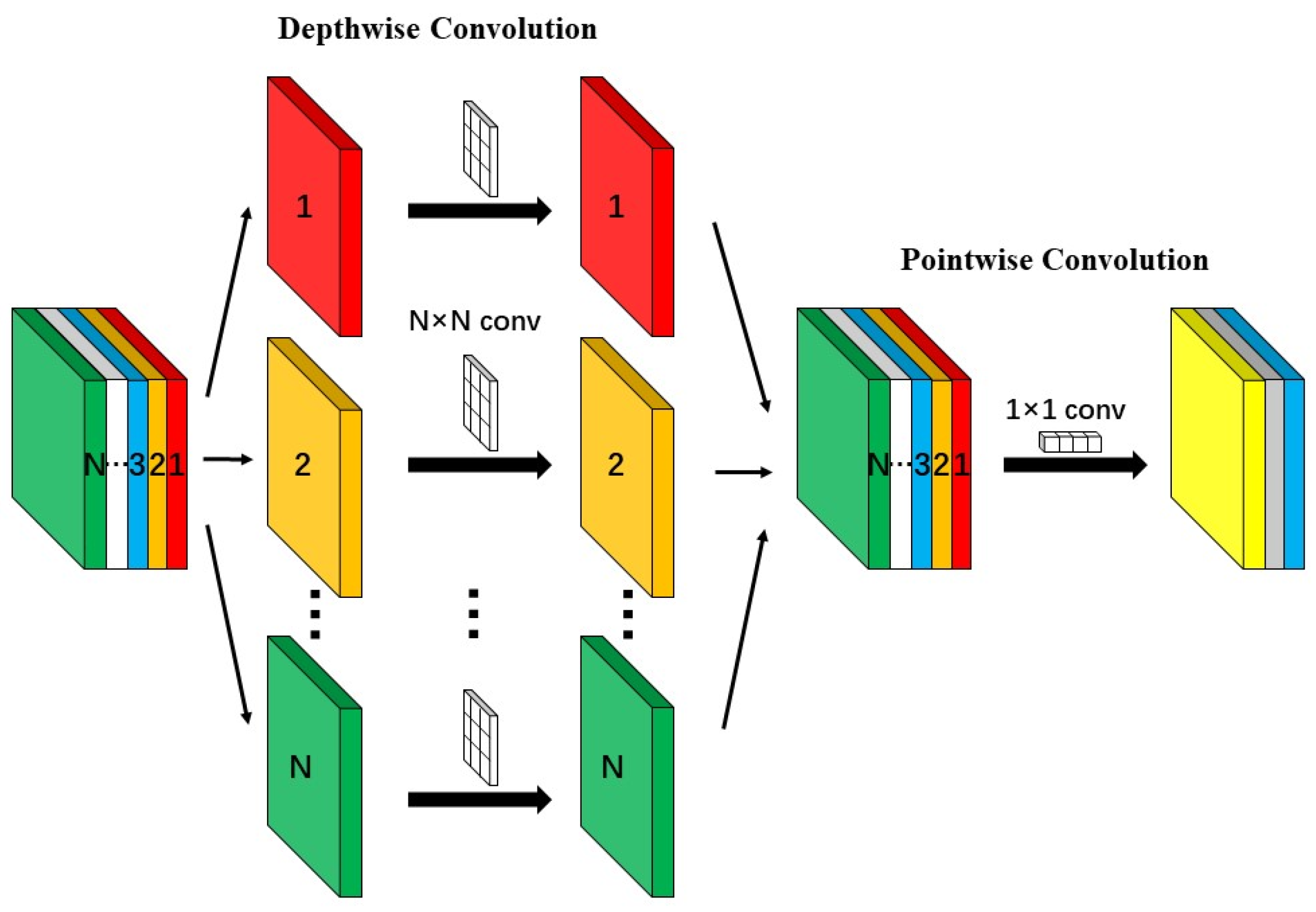
  • Depthwise separable convolutions were utilized as the feature extraction module in the backbone network, reducing model parameters, the computation required for convolution operations, and network inference latency.
  • A new plug-and-play module, FC-C2f, was designed to optimize the backbone network structure, reduce computational redundancy, and lower the model’s parameters and FLOPs.
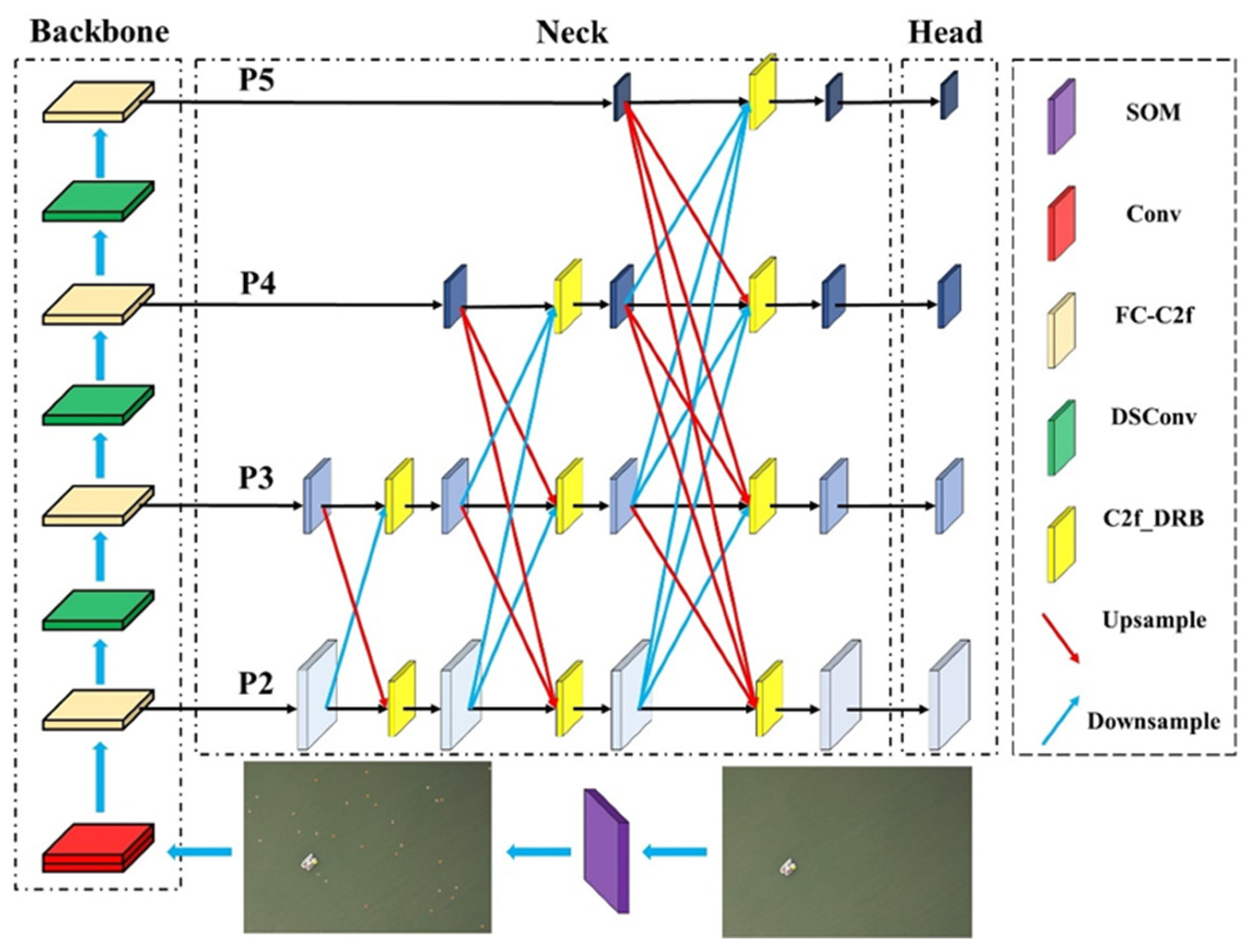
• A new multiscale fusion network, LMFN, was designed to address the accuracy issues in multiscale object recognition.
  • By gradually integrating features from different levels, the connections between layers are effectively increased, and the model’s feature fusion process is optimized. This enhances the model’s capability to fuse multiscale features, improving detection accuracy for objects of various scales.
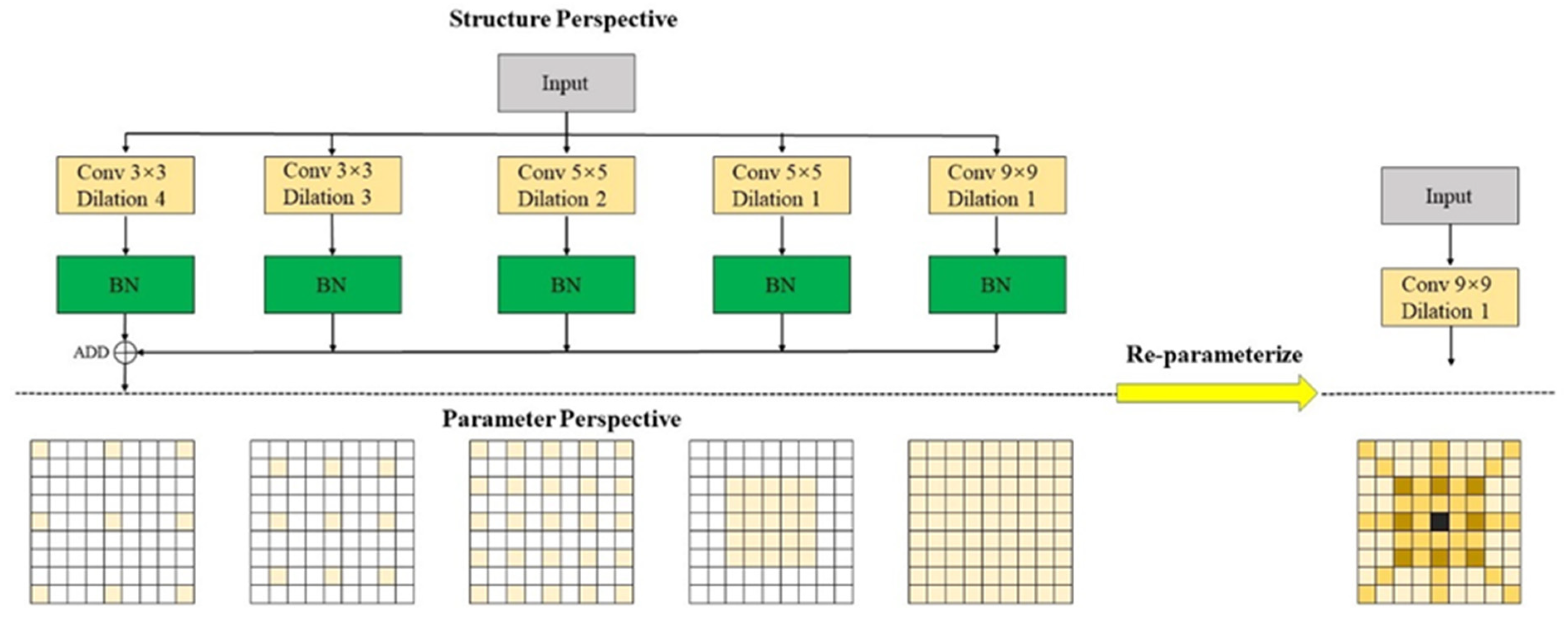
  • Combined dilated convolutions with small kernels and cascaded convolutions into a re-parameterized large kernel convolution. This approach retains the benefits of small kernels, such as reduced computational load and fewer parameters, while achieving the large effective receptive field of large kernels. The experimental results demonstrate that this structure reduces model parameters and increases the receptive field.

2. Related Work

2.1. Data Augmentation

Depending on the application scenarios and the characteristics of the different datasets, using appropriate data augmentation algorithms can enhance the model’s detection accuracy and robustness. In some datasets, the number of samples in certain classes may be significantly higher than in others, a phenomenon known as class imbalance. Class imbalance adversely affects the model’s convergence speed and detection accuracy, impacting both training convergence and generalization on the test set. To address class imbalance in the training set, the most common methods can be divided into two categories: data-level methods that directly manipulate the dataset to change class distribution and classifier-level methods. Methods for addressing class imbalance through classifier optimization include cost-sensitive learning, adjusting decision thresholds, weighted loss functions, ensemble methods, and feature learning. These approaches assign different misclassification costs, optimize loss functions, and design specific network structures, thereby increasing the model’s focus on minority class data. Data-level methods address class imbalance by adjusting the distribution of the dataset, including techniques such as oversampling, undersampling, data synthesis, and data augmentation. These techniques aim to balance class proportions in the dataset, enabling the model to better learn features of the minority class, thereby enhancing performance and generalization. Although classifier optimization methods offer precise control over model behavior, they are complex and resource-intensive, making them unsuitable for the application scenario of this paper. Data-level methods directly modify data distribution, are simple to implement, and can increase the quantity and diversity of minority class samples through oversampling, undersampling, and data augmentation, improving the model’s ability to recognize minority classes. Given that the YOLO algorithm requires a substantial amount of training data to effectively fit the network, this paper utilizes oversampling to increase the number of minority class samples.

Chen et al. proposed a multi-sample data augmentation method for remote sensing images called SSMup [20], which integrates three data augmentation techniques: Mosaic, Mixup, and SSMOTE. This algorithm ensures the uniform distribution of objects in the enhanced samples and provides rich background information. Zhang et al. proposed a novel grid-oversampling strategy [21]. This strategy first uses the OSTU algorithm for feature extraction before cropping, then crops the image using a sliding window, and finally retains only objects that occupy more than 80% of the sliding window’s foreground. This approach accelerates the detection speed of sparse object images. This strategy can speed up sparse object detection in sparse object images. In the SeaDroneSee dataset, even objects with the same label category can have vastly different characteristics. As shown in Figure 1, both images have objects labeled as “life_saving_appliances”, but in Figure 1a, the objects are a lifebuoy and a float board, while in Figure 1b, the object is a life jacket. Therefore, simply using the Simple Copy-Paste [22] data augmentation algorithm to increase the number of objects is unlikely to yield satisfactory results. Additionally, the marine environment is complex and variable, with significant background differences between images. Copy-paste operations across multiple images can easily lead to image distortion due to large discrepancies between the pasted region and the original image background. Additionally, excessive oversampling may lead to model overfitting. To address these issues, this paper proposes the SOM data augmentation algorithm based on oversampling. The SOM data augmentation algorithm utilizes a Gaussian filter to smooth the edges of pasted objects, mitigating the image distortion caused by copy-paste operations. To prevent overfitting due to excessive oversampling, the SOM algorithm restricts oversampling to small objects with fewer than 32 × 32 pixels, thereby excluding larger objects within the same class from oversampling. Since small objects occupy a small pixel area and yield fewer extracted features, oversampling these small objects is less likely to result in overfitting.

2.2. Lightweight Methods for Object Detection Networks Based on Deep Learning

In open water search and rescue missions, it is crucial to make lightweight improvements to existing object detection models due to the limited power consumption and computational resources available of UAVs. Lightweight network architectures originated from SqueezeNet [23] in 2016 and MobileNet [24] in 2017. These networks have since seen multiple improved versions, such as SqueezeNext [25] and MobileNetV2-4 [26,27,28]. SqueezeNet introduces the Fire module, which uses multiple 1 × 1 convolution kernels connected instead of 3 × 3 convolution kernels. By adjusting the number of 1 × 1 convolutions, the number of channels in each layer can be flexibly controlled, reducing both model parameters and computational load. The MobileNet series algorithms proposed depthwise separable convolution, dividing standard convolution operations into two processes: depthwise convolutions followed by pointwise convolutions. This approach significantly reduces parameters and computational load, accelerating both model training and inference speed.

In addition to designing lightweight networks, many researchers have focused on creating lightweight designs for specific parts of existing object detection networks. Zhang et al. introduced a lightweight improvement to the detection head, proposing a Lightweight Asymmetric Detection Head (LADH-Head) [29]. LADH-Head utilizes depthwise separable convolution to optimize the Asymmetric Decouple Head (ADH), significantly reducing model parameters while improving detection accuracy. Wenkai Gong has proposed a lightweight feature extraction module called Dynamic Group Convolution Shuffle Transformer (DGST) to further enhance computational efficiency and performance [30]. DGST incorporates group convolution to reduce model parameters and computational load while preventing overfitting. It also integrates the channel shuffle technique from ShuffleNetV2 to promote effective inter-group feature information exchange. Additionally, DGST incorporates Vision Transformer, further improving computational efficiency and performance. Wang et al. introduced a plug-and-play feature upsampling module Content-Aware ReAssembly of Features (CARAFE) [31]. Instead of using a fixed kernel, CARAFE can dynamically generate adaptive kernels by performing content-aware processing on specific instances. In addition, CARAFE has a low computational overhead and can be easily integrated into other network architectures.

2.3. MultiScale Feature Fusion

In object detection algorithms, the neck network is commonly utilized to combine different layers of feature maps extracted from the backbone network. This fusion generates feature maps with multiscale information, which enables the enhancement of the accuracy of object detection. The introduction of Feature Pyramid Networks (FPN) in 2016 was a milestone, addressing the shortcomings of detection networks in handling multiscale variations [32]. Building on FPN, Liu et al. proposed the Path Aggregation Network (PANet) [33]. PANet enhances the feature hierarchy with a bottom-up path, leveraging precise positional information from lower-level feature layers to strengthen higher-level feature layers.

Xu et al. proposed an efficient Reparameterized Generalized Feature Pyramid Network (RepGFPN) [34]. The RepGFPN enhances feature interaction through queen-fusion and reduces the extra upsampling in post-fusion to decrease model complexity. It also introduces a re-parameterization mechanism and efficient layer aggregation networks (ELAN) to upgrade the feature fusion module, achieving higher accuracy without additional computational burden. Tan et al. designed a Bi-Directional Feature Pyramid Network (BiFPN) [35] that achieves efficient bidirectional cross-scale connections and weighted feature fusion. Li et al. introduced a lightweight Context and Spatial Feature Calibration Network (CSFCN) [36]. CSFCN consists of two main parts: the Context Feature Calibration (CFC) module and the Spatial Feature Calibration (SFC) module. The CFC module calculates the similarity between pixels and their context, aggregating the context of each pixel’s related semantics to achieve context feature calibration, thereby alleviating context mismatch issues. The SFC module groups channels into multiple sub-features along the spatial dimension and calibrates them separately to address feature misalignment problems.

3. Materials and Methods

The combination of object detection algorithms and UAV technology is significant for improving detection efficiency, ensuring regional safety, and reducing resource consumption. The YOLOv8 model comes in five versions, with parameters increasing in size from n, s, m, l, to x; larger models offer higher detection accuracy. Considering detection accuracy, model size, and practical application needs, this paper selects the YOLOv8s algorithm as the baseline model. Although the original YOLOv8s algorithm outperforms YOLOv8n in detection performance, its parameter count is 3.5 times greater, reaching 11.2 M. Therefore, this paper proposes a lightweight improvement to the YOLOv8s algorithm, designing a lightweight object detection algorithm for aerial images in open waters, named DFLM-YOLO. Section 3.1 details the SOM data augmentation algorithm for optimizing and enhancing the dataset. Section 3.2 and Section 3.3 focus on lightweight improvements to the backbone network. Section 3.4 discusses the redesign of the neck network. The network structure of the DFLM-YOLO model is shown in Figure 2.

3.1. Small Object Multiplication Data Augmentation Algorithm

In deep learning, the balance of the dataset is crucial for model training. If the number of samples in one class is significantly lower than in other classes, the model may become biased towards the more numerous classes during training, reducing its ability to classify the less represented classes. The experimental data for this paper come from the SeaDroneSee public dataset. SeaDroneSee was collected by the University of Tuebingen team to assist in the development of search and rescue systems using UAVs in maritime scenarios. It was collected using the fixed-wing aircraft Trinity F90+ and other quadrotor drones over Lake Constance. The Trinity F90+ is manufactured by Quantum-Systems GmbH, a company based in Gilching, Germany. It is an electric vertical take-off and landing (eVTOL) fixed-wing drone, widely recognized for its long flight endurance and professional-grade capabilities. Video data were captured and several frames were extracted and annotated to create the dataset. The images in the dataset have a resolution of approximately 1230 × 930 pixels. The dataset comprises 8930 training images, 1547 validation images, and 3750 test images. These images include various lighting conditions, different shooting distances, and angles, meeting factors such as small object size and complex environments. There are five categories in the dataset: swimmer, boat, buoy, jetski, and life_saving_appliances. This dataset provides a valuable data resource for maritime search and rescue in open waters. We conducted a statistical analysis of the training set of the SeaDroneSee dataset, with the results shown in Figure 3a. The pie chart reveals that the “life-saving appliances” category contains only 923 instances, making up just 1.6% of the total objects, while the most abundant category, “swimmer”, has 37,096 instances, accounting for 64.22%. Due to the scarcity and small size of “life-saving appliances”, their recall rate in the YOLOv8s algorithm’s detection results is only 14.5%, as shown in Table 4. Additionally, Figure 3b presents the statistics of the number of objects in each category of the dataset after data augmentation. It can be seen from this figure that the dataset is nearly balanced across categories after data augmentation.

Inspired by SSMup, Simple Copy-Paste, and Augmentation for small object detection [37], this paper proposes a data augmentation algorithm called Small Object Multiplication (SOM). This algorithm balances the dataset by increasing the number of small objects in specific categories through oversampling, thereby addressing the low detection performance caused by class imbalance. Due to the small pixel size of the objects and the limited features extracted by the model, oversampling is performed only on objects smaller than 32 × 32 pixels to prevent model overfitting from excessive oversampling. Additionally, the SOM data augmentation algorithm incorporates a Gaussian filter to smooth the edges of pasted objects, addressing the image distortion caused by copy-paste operations. We illustrate the steps of the SOM data augmentation algorithm in Algorithm 1. Here, I_N represents the N-th image in the training set, A_N corresponds to its annotation information, L denotes the object category index to be duplicated, and n is the number of duplications. The image, annotation information, desired object category index, and number of duplications are used as the input variables for the algorithm. In the first step, the algorithm checks if the object category exists in the annotation file and whether its size is smaller than 32 × 32. If these conditions are met, the object information is saved to List 1. In the second step, based on the duplication count n and the object size information, n paste regions are randomly generated in the original image and the corresponding object pixel information from the list is pasted. In the pseudocode, X and Y represent the image’s width and height, respectively. The paste function performs the oversampling operation, primarily pasting the object pixel information at specified coordinates. The Add_New_Annotation function adds the new sample’s annotation information generated using the oversampling operation to the original annotation file. SOM_Image refers to the image after the oversampling operation, and SOM_Annotation refers to the annotation file after the operation. The object information refers to the image area of the pasted object. Finally, a Gaussian filter is applied to smooth the oversampled image, particularly around the edges of the pasted areas.

Algorithm 1: The Working Steps of the SOM Data Augmentation Algorithm

Input: Image (IN), Annotation (AN), Object category index (L), Copy-Paste times (n).  Step 1: Iterate through the annotation information (AN) and check if there are any objects with the category index L and if their pixel size is smaller than 32 × 32. If these conditions are met, save the size and pixel information of these objects in List 1.   for class_number in AN:     if (class_number == L) and (object size < 32 × 32):      List1.append(AN [class_number])     else:       continue  Step 2: The paste regions are randomly generated in the original image according to the number of duplications and their suitability is assessed. If unsuitable, new regions are generated. The qualifying object areas are pasted into these regions, and the annotation information for the newly generated objects is added to the annotation file.   for object information in List1:    for i in range(0, n):     top-left coordinates = random(0, X), random(0, Y)     bottom-right coordinates = top-left coordinates(x, y)—object size     if bottom-right coordinates(x) > X or bottom-right coordinates(y) > Y:        n = n – 1        continue     SOM_Image = Paste(top-left coordinates, bottom-right coordinates, object information)     SOM_Annotation = Add_New_Annotation(class number, object coordinates)  Step 3: Use a Gaussian filter to smooth the edges of the pasted objects. The Blurred_image is the image after Gaussian smoothing, while GaussianBlur is the Gaussian filter applied to the entire image, particularly to the edges of the pasted regions.   Blurred_image = GaussianBlur(SOM_Image, Gaussian kernel size, Gaussian kernel standard deviation)  Output: The image after SOM data augmentation, Blurred_image, and the corresponding annotation file, SOM_ Annotation.

3.2. Depthwise Separable Convolution

The backbone network of the YOLOv8s algorithm accounts for approximately 45% of the overall parameters, with its complex convolutional structures leading to an excessive number of model parameters. This increases the demand for hardware computational power and memory, posing challenges for resource-limited mobile computing terminals to perform object detection tasks. To address this problem, inspired by the classic MobileNet lightweight network family, this paper uses DSConv [38] to make lightweight improvements to the YOLOv8s backbone network. The detailed structure of DSConv is shown in Figure 4.

We will now analyze and compare the computational requirements for performing a convolution operation using standard convolution and DSConv. Let us assume that the input feature map size is $h\times w\times c$, the size of the convolution kernel is $k\times k\times c$, and the total number of kernels is N. The spatial dimension of the feature map contains a total of $h\times w$ points. The computation required to perform the convolution operation for each point is equivalent to the size of the convolution kernel. If we perform one convolution operation for each point at every spatial location in the feature map, then a single convolution would require a total $h\times w\times c\times k^2$ of computations. In the analogous analysis, the number of calculations required in the DWConv stage is also $h\times w\times c\times k^2$. The number of calculations required in the Pointwise Convolution (PWConv) process is $h\times w\times c\times N$; the DSConv is: $h\times w\times c\times k^2+h\times w\times c\times N$. From this, the total number of calculations for the N standard convolutions is $h\times w\times c\times k^2\times N$. We can derive the ratio of the total number of calculations for the DSConv and the standard convolutions as follows: ${\displaystyle \frac{1}{N}}+{\displaystyle \frac{1}{k^2}}$. In summary, the computational efficiency of DSConv is far superior to that of the standard convolutions, which can reduce the model parameters and reduce the network inference delay, which is conducive to the lightweight design of the model. The computational efficiency is much better than the standard convolution, which can reduce the model parameters, reduce the network inference delay, and is conducive to the lightweight design of the model.

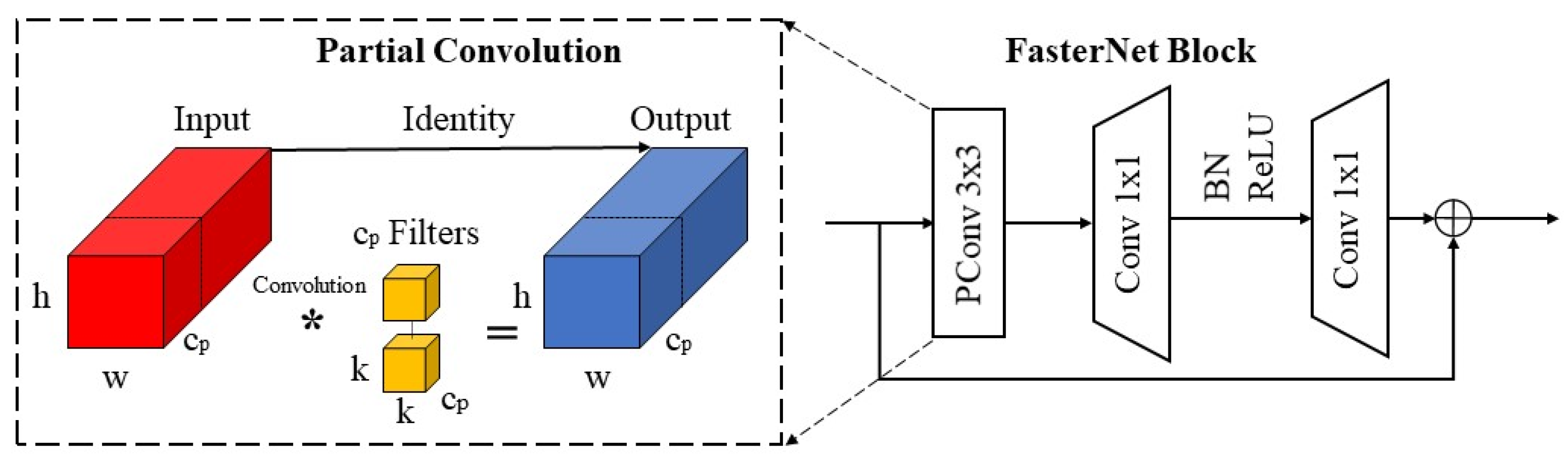
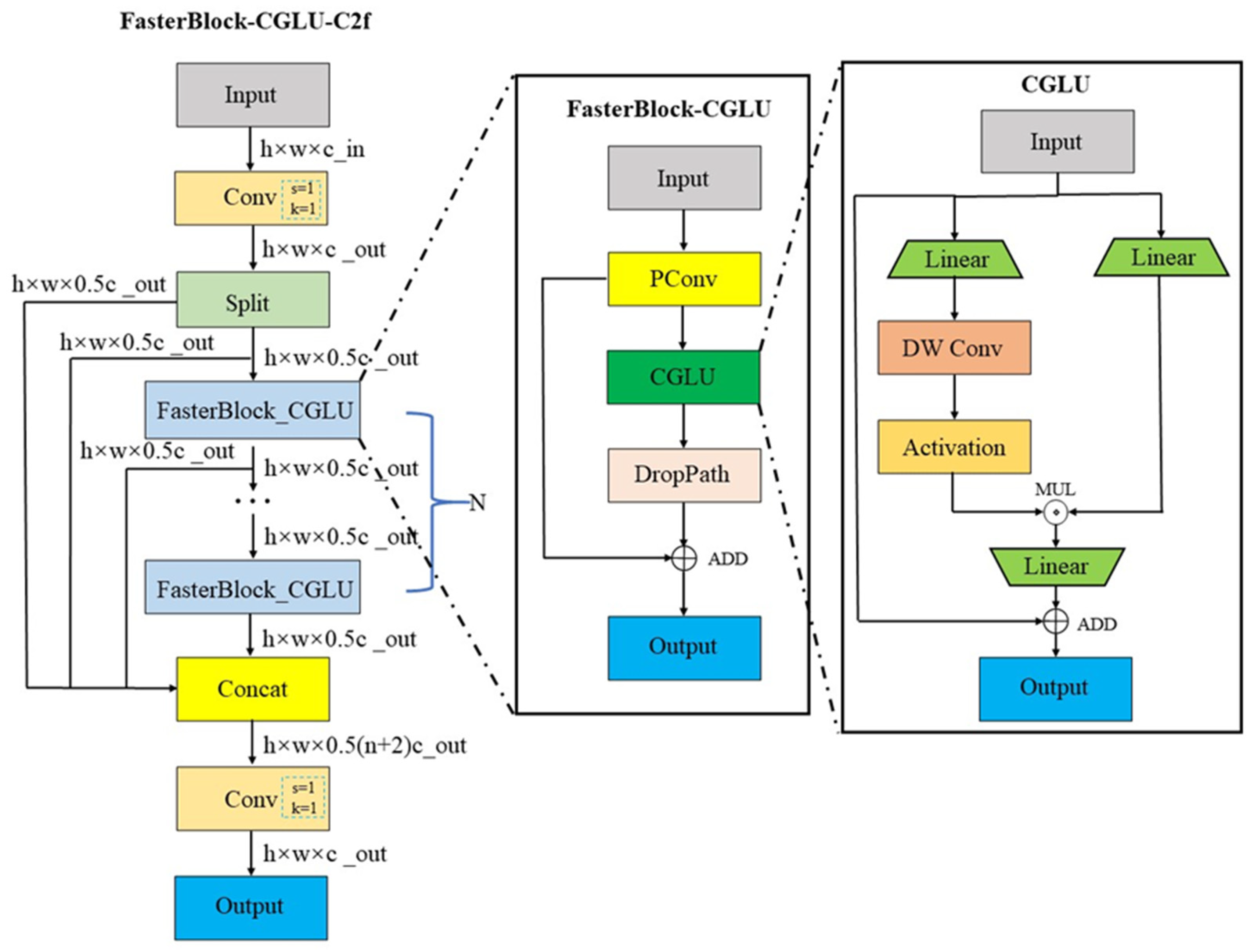
3.3. Improved C2f Module Based on Convolutional Gated Linear Unit and Faster Block

In the original YOLOv8s’ backbone network, the convolution module only accounts for 30% of the total parameters, while the C2f module accounts for 56%. Therefore, this paper draws inspiration from the FasterBlock module in FasterNet [39] to make lightweight improvements to the C2f module in the backbone network. FasterNet is a fast neural network that was proposed by Jierun Chen et al. in 2023. The model delay is calculated as $Latency={\displaystyle \frac{FLOPs}{FLOPS}}$. Chen et al. discovered that many researchers focus on accelerating models by reducing FLOPs, such as ShuffleNets [40] and GhostNet [41]. However, this reduction in FLOPs can lead to increased memory access, resulting in higher network latency and affecting computational speed. This explains why some models have low FLOPs but still exhibit slow inference and run times. We encountered a similar situation in our experiments when replacing the original YOLOv8s backbone with HGNetV2 [42]. Although FLOPs decreased by 19%, there was almost no change in inference speed, as shown in

Table 1. The influence of replacing the YOLOv8s backbone with HGNetV2 on the SeaDroneSee-val.

Algorithms	FLOPs (G)	Pre-Process (ms)	Inference (ms)	NMS (ms)
YOLOv8s	28.8	0.2	1.6	0.8
YOLOv8s + HGNetV2	23.3	0.2	1.6	0.7

. Pre-Process refers to the pre-processing time during model inference, Inference is the time taken for inference, and Non-Maximum Suppression (NMS) is the post-processing time.

To reduce memory access and computational redundancy, Chen et al. proposed a new convolutional structure called Partial Convolution (PConv) and designed the FasterNet block based on Pconv. The working principle of Pconv and the model structure of the FasterNet block are illustrated in Figure 5. As depicted in Figure 5, Pconv utilizes the standard convolution to extract spatial features from a portion of the input channel while leaving the rest of the channel unchanged. This process significantly reduces computational redundancy and enhances the inference speed. We use the same method as in the previous subsection to calculate the computation of Pconv; assuming that the size of the input feature map is $h\times w\times c$, $c_p$ is the number of feature map channels participating in the convolution operation, the size of the convolution kernel is $k\times k\times c$, and it is the number of $c_p$. We can derive the total computation amount of Pconv as $h\times w\times c_p^2\times k^2$. In summary, the ratio of the total computational load of Pconv to that of the standard convolution is $\frac{c_p^2}{c\times N}$.

Although the improved C2f module reduces the model parameters by 13%, inference is still slow because Conv extracts features through serial operations. The Gated Linear Unit (GLU) [43] was proposed in 2016 by Yann N. Dauphin et al. The GLU consists of two linear projections, one of which is controlled by a gating function, and the two projections are multiplied elementwise. The GLU can accelerate computation speed and reduce the model’s complexity through a parallel processing structure. Subsequently, Dai Shi proposed an improved GLU call Convolutional GLU (CGLU) [44]. This new model innovatively combines depthwise convolution using parallel processing structures to enhance computation speed and reduce model complexity. Additionally, the depthwise convolution structure provides positional information and efficient feature extraction capabilities. Inspired by FasterBlock and CGLU, this paper improves the C2f structure in the YOLOv8s backbone and proposes the FasterBlock-CGLU-C2f (FC-C2f) module. The structure of the FC-C2f module is shown in Figure 6.

3.4. Lightweight Multiscale Feature Fusion Network

The uncertainty of the object size in aerial images can lead to the loss of information during feature extraction, which affects the model’s detection performance. The YOLOv8 algorithm utilizes Feature Pyramid Network (FPN) and Path Aggregation Network (PAN) structures for downsampling and upsampling, respectively. These structures have large parameter counts, high computational redundancy, significant conflicts between different feature levels, and a relatively limited effectiveness in detecting small objects. The neck network of the YOLOv8s algorithm has approximately 6.06 M parameters, making it challenging to deploy on an airborne computation device. Therefore, this paper designs a lightweight multiscale fusion network (LMFN). The architecture of LMFN is shown in Figure 7.

LMFN adopts the progressive fusion strategy of the Asymptotic Feature Pyramid Network (AFPN) [45], which integrates the shallow and deep features extracted using the backbone network in three stages. This fusion method weights the semantic and positional information of deep and shallow features according to different feature levels, avoiding significant semantic gaps between different feature layers and preventing information loss and degradation caused by multi-level transmission.

The receptive field can be expanded by connecting multiple small-kernel convolutions or by using a single large-kernel convolution. Researchers typically prefer the first method because using multiple small-kernel convolutions has three advantages over a single large-kernel convolution. Firstly, multiple small-kernel convolution structures include more non-linear activation layers, thereby enhancing the discriminative ability of the model. Secondly, it reduces network parameters. For example, using three 3 × 3 cascade convolutions instead of a single 7 × 7 large kernel convolution can reduce 7 × 7 − 3 × 3 × 3 = 22 parameters, cutting the network parameters by 45%. Lastly, it also decreases the computational load. Similarly, using three 3 × 3 cascade convolutions instead of a single 7 × 7 large kernel convolution can reduce the number of computations by 7 × 7 × C − 3 × 3 × 3 × C = 22 × C, reducing the computational load by 45%.

Ding et al. found that although connecting multiple small-kernel convolutions can theoretically expand the model’s maximum receptive field, the actual effective depth is not significant, resulting in a small Effective Receptive Field (ERF) [46]. The ERF is proportional to $O\left(K\sqrt{L}\right)$, where K represents the kernel size and L is the model depth [47]. This indicates that the ERF is more sensitive to changes in K. Although the optimization problems brought by increasing model depth have been addressed by ResNet, increasing the depth of the model is not as effective as increasing the kernel size.

To achieve a large ERF and fully utilize deep features while avoiding the increase in network parameters and computational load caused by large-kernel convolutions, this paper designs a new C2f module named DRB-C2f. The Dilated Re-param Block (DRB) [48] module utilizes parallel dilated convolution in addition to the large kernel convolution. Using the concept of re-parameterization, the entire module can be considered a non-dilated large kernel convolution. The operational diagram is depicted in Figure 8. The ignored pixels in dilated convolution can be considered as adding extra zero terms to the convolution kernel. Therefore, a dilated convolution layer with a small convolution kernel can be seen as a non-dilated convolution layer with a larger but sparser kernel. The process of adding zeros can be carried out using transposed convolution with a step size r and a unit kernel $I\in {ℝ}^{1\times 1}$. If the original convolution kernel is $I\in {ℝ}^{1\times 1}$, the convolution kernel after the interpolation operation is $W^{\prime }\in {ℝ}^{\left(\right(k-1)r+1)\times \left(\right(k-1)r+1)}$. The re-parameterize module consists of a non-diluted small convolution kernel and multiple diluted small convolution kernels to complement the non-diluted large convolution kernel.

We utilized the visualization tool Zetane to display the feature maps in the dashed section of Figure 7. Figure 9 illustrates the changes in the four feature layers before and after implementing DRB. The left side displays the size of the feature maps without DRB enhancement, while the right side shows the size of the feature maps after incorporating DRB enhancement. In the figure, “Shape” represents the number of channels and dimensions of the layer, “Mean” indicates the average receptive field size, “Stdev” denotes the standard deviation of the receptive field distribution, and the colored section on the right is a histogram of the receptive field distribution range. This figure indicates that using DRB significantly increases the size of the model’s receptive field. The mean receptive field size increased from 0.305, 1.63, 1.77, and 6.28 to 0.879, 3.15, 2.7, and 12.7 for P2, P3, P4, and P5, respectively.

4. Experimental and Analysis

4.1. Experimental Environment and Parameter Settings

In the experiments, we used the SeaDroneSee public dataset as the training metadata for the model. The hardware environment for training the model included an NVIDIA GeForce RTX 4090 GPU and an Intel(R) Xeon(R) Gold 6430 CPU. The software environment consisted of Ubuntu 20.04 as the operating system, along with Python 3.8, PyTorch 1.10.0, and CUDA 11.3. The hardware configurations and software versions involved in this experiment are shown in

Table 2. Hardware model and software version used for the experiment.

Experimental Environment	Parameter/Version
Operating System	Ubuntu20.04
GPU	NVIDIA Geforce RTX 4090
CPU	Intel(R) Xeon(R) Gold 6430
CUDA	11.3
PyTorch	1.10.0
Python	3.8

. Based on the aforementioned computer configuration, we set the input image size to 640 × 640 pixels, the batch size to 16, and the number of training epochs to 200. All other hyperparameters were set to their default values. Additionally, all models mentioned in this paper were trained from scratch without loading any pre-trained weights. The hyperparameter settings of the model are shown in

Table 3. Network model hyperparameter settings.

Parameter	Setup
Image size	640 × 640
Momentum	0.937
BatchSize	16
Epoch	200
Initial learning rate	0.01
Final learning rate	0.0001
Weight decay	0.0005
Warmup epochs	3
IoU	0.7
Close Mosaic	10
Optimizer	SGD

.

4.2. Experimental Metrics

To objectively evaluate the model’s performance, this paper measures and analyzes it from two aspects: detection performance and detection speed. The quantitative metrics for detection performance include Precision, Recall, mAP50, Parameters, and FLOPs. The quantitative metric for detection speed is the total inference time for a single image with a batch size set to 16.

The Precision measures the ratio of correctly predicted objects to the total number of predicted objects using the following Formula (1):

$$P={\displaystyle \frac{TP}{TP+FP}},$$

(1)

Recall measures the ratio of correctly predicted objects to the number of actual objects. The calculation formula is as follows (2):

$$R={\displaystyle \frac{TP}{TP+FN}},$$

(2)

In the formulas, TP (True Positives) is the number of objects correctly identified using the model, FP (False Positives) is the number of other class objects incorrectly identified as this class, and FN (False Negatives) is the number of the class objects incorrectly identified as other classes. Thus, $TP+FP$ represent the number of objects predicted using the model, while $TP+FN$ represent the actual number of such objects.

The mean average precision (mAP) is the average of the average precision (AP) values for multiple categories and is used to measure the overall performance of the model. The mAP50 is the mAP at an IoU threshold of 50%. The mAP50-95 is the mAP calculated at IoU thresholds ranging from 50% to 95% in 5% increments, yielding ten mAP values. The final mAP is the average of these ten values. The specific IoU thresholds used are [50%, 55%, 60%, 65%, 70%, 75%, 80%, 85%, 90%, 95%]. The calculation Formula (3) for mAP is as follows:

$$mAP=\frac{{\displaystyle \sum _{n=1}^N}A{P}_n}{N},$$

(3)

where $A{P}_n$ refers to the average precision of the nth class of objects, used to evaluate the model’s detection performance for that specific class. The calculation Formula (4) is as follows:

$$AP={\int }_0^{1}PRdR,$$

(4)

The parameter count represents the total number of parameters in the model, which is a key indicator of the model’s size and spatial complexity. It directly impacts the size of the weight file and indirectly affects the storage space required for model deployment. The FLOPs measures the computational load required during model training and inference, reflecting the model’s computational efficiency.

4.3. Ablation Experiments

4.3.1. The Effect of SOM Data Augmentation on the Original Model

In this paper, the small objects labeled as “boat”, “jetski”, “life_saving_appliances”, and “buoy” were subject to copy-paste operations 2, 7, 39, and 15 times, respectively. Figure 10 displays an example image before and after applying the SOM data augmentation algorithm, with some areas of this figure enlarged. From the figure, it is evident that two different “life-saving appliances” were duplicated 39 times and randomly pasted onto the original image.

The experimental results for the SeaDroneSee dataset are shown in

Table 4. The influence of the SOM data augmentation algorithm on SeaDroneSee-val. The three columns on the left represent the original YOLOv8s detection results, while the three columns on the right show the detection results after applying the SOM data augmentation.

Algorithms	YOLOv8s			YOLOv8s + SOM
Classes	P(%)	R(%)	mAP(%)	P (%)	R(%)	mAP(%)
swimmer	78.7	66.5	69.6	80.1 (+1.4)	64.8 (−1.7)	70.3 (+0.7)
boat	89.8	86	91.6	89.9 (+0.1)	87.4 (+1.4)	91.2 (+0.4)
jetski	76.8	82.2	83.7	86.3 (+9.5)	82.5 (+0.3)	84.6 (+0.9)
life_saving_appliances	78.2	14.5	28.2	81 (+2.8)	25.5 (+11)	35.4 (+6.9)
buoy	77.7	50.5	57.2	88.5 (+10.8)	51.6 (+1.1)	61.4 (+4.2)
All	80.2	59.9	66.1	85.2 (+5)	62.4 (+2.5)	68.6 (+2.5)

. Combining the results from Figure 10 and Table 4, it can be seen that the more copy-paste operations performed for a category, the greater the mAP increase. The “life_saving_appliances” category shows the most significant improvement, with the accuracy rate increasing from 78.2% to 81%, the recall rate increasing from 14.5% to 25.5%, and the mAP increasing from 28.2% to 35.4%. Therefore, the SOM data augmentation algorithm can effectively address the low recall and accuracy rates caused by the lack of object samples, resolving the class imbalance problem in the dataset.

4.3.2. The Effect of DSConv on the Original Model

The experimental results for the SeaDroneSee dataset before and after lightening the backbone network using DSConv are presented in

Table 5. The influence of DSConv on SeaDroneSee-val.

Algorithms	P (%)	R (%)	mAP50val (%)	Params (M)	FLOPs (G)	Speed RTX4090 b16 (ms)
YOLOv8s	80.2	59.9	66.1	11.14	28.7	2.6
YOLOv8s + DSConv	79.8 (−0.4)	60.5 (+0.6)	66.6 (+0.5)	9.59 (−1.55)	25.7 (−3)	1.2 (−1.4)

. The improved backbone network with the DSConv module reduces the model’s parameters by 13.9%, FLOPs by 10.5%, and decreases the inference time from 2.6 ms to 1.2 ms, resulting in a 53.85% improvement. Additionally, there is a slight improvement in detection accuracy. These results indicate that DSConv can enhance the computational efficiency of the model, decrease the model’s inference time, and improve detection accuracy.

4.3.3. The Effect of FC-C2f on the Original Model

The experimental results on the SeaDroneSee dataset are shown in

Table 6. The influence of FasterBlock and FasterBlock-CGLU-C2f on SeaDroneSee-val.

Algorithms	P (%)	R (%)	mAP50val (%)	Params (M)	FLOPs (G)	Speed RTX4090 b16 (ms)
YOLOv8s	80.2	59.9	66.1	11.14	28.7	2.6
YOLOv8s + FB-C2f	80.4 (+0.2)	61.2 (+1.3)	66.1 (+0)	9.69 (−1.45)	24.4 (−4.3)	2.2 (−0.4)
YOLOv8s + FC-C2f	82.8 (+2.6)	59.5 (−0.4)	66.5 (+0.4)	9.48 (−1.66)	23.8 (−4.9)	1.4 (−1.2)

, where FB-C2f is the improved C2f module using only FasterBlock. From Table 6, we can conclude that the FC-C2f module improved with CGLU can further optimize the network structure compared to the FB-C2f module. It not only enhances detection accuracy but also makes the network lighter, increasing the model’s detection speed and proving the effectiveness of the CGLU improvement. The improved FC-C2f module reduces the model’s parameters by 17.5%, FLOPs by 17.1%, and inference time from 2.6 ms to 1.4 ms, a reduction of 46.2%, with a slight improvement in detection accuracy. The proposed FC-C2f module can increase detection accuracy while reducing model parameters, lowering model complexity, and significantly improving the model’s running speed.

4.3.4. The Effect of LMFN on the Original Model

The experimental results on the SeaDroneSee dataset are shown in

Table 7. The influence of AFPN, AFPN_C2f, and LMFN on SeaDroneSee-val.

Algorithms	P (%)	R (%)	mAP50val (%)	Params (M)	FLOPs (G)	Speed RTX4090 b16 (ms)
YOLOv8s	80.2	59.9	66.1	11.14	28.7	2.6
AFPN	83.2 (+3.0)	71.4 (+11.5)	76.3 (+10.2)	8.76 (−2.38)	38.9 (+10.2)	3.1 (+0.5)
AFPN_C2f	84.5 (+4.3)	69.6 (+9.7)	76.0 (+9.9)	7.09 (−4.05)	34.2 (+5.5)	2.8 (+0.2)
LMFN	86.8 (+6.6)	70.5 (+10.6)	76.7 (+10.6)	6.86 (−4.28)	31.1 (+2.4)	2.3 (−0.3)

. AFPN_C2f is the neck network that is not improved with DRB. From this table, we can see that AFPN_C2f achieves lightness at the expense of accuracy. The DRB module introduction improves the multiscale feature fusion network, increasing the model’s effective receptive field and detection accuracy, while reducing the model’s parameters and FLOPs. Compared to YOLOv8s, mAP50 is improved by 10.6%, and the number of parameters is reduced by 38.4%. However, due to the extensive multiscale fusion operations, FLOPs increased by 7.7%. Compared to AFPN, the detection accuracy of LMFN did not decrease but improved by 0.4%, and the number of parameters and FLOPs decreased by 21.7% and 20%, respectively. Overall, the enhanced LMFN exhibits significant superiority.

4.3.5. The Effect of Combining Multiple Improvement Modules on the Original Model

In this study, we propose four improvement methods for YOLOv8s aimed at reducing model parameters, increasing detection speed, and enhancing the detection accuracy for small objects. The four improvement methods include the following: (a) utilizing the SOM data augmentation algorithm to improve dataset balance, (b) using DSConv instead of standard convolutions in the backbone network for lightweight design, (c) improving the C2f module in the backbone network using FasterBlock and GSLU to reduce parameters and latency, and (d) redesigning the neck network with the LMFN to increase the effective receptive field and multiscale feature fusion capability. To study and analyze the effectiveness of each improvement method in depth, we conducted ablation experiments on the SeaDroneSee dataset. The results are shown in

Table 8. The influence of different improvements evaluated on SeaDroneSee-val.

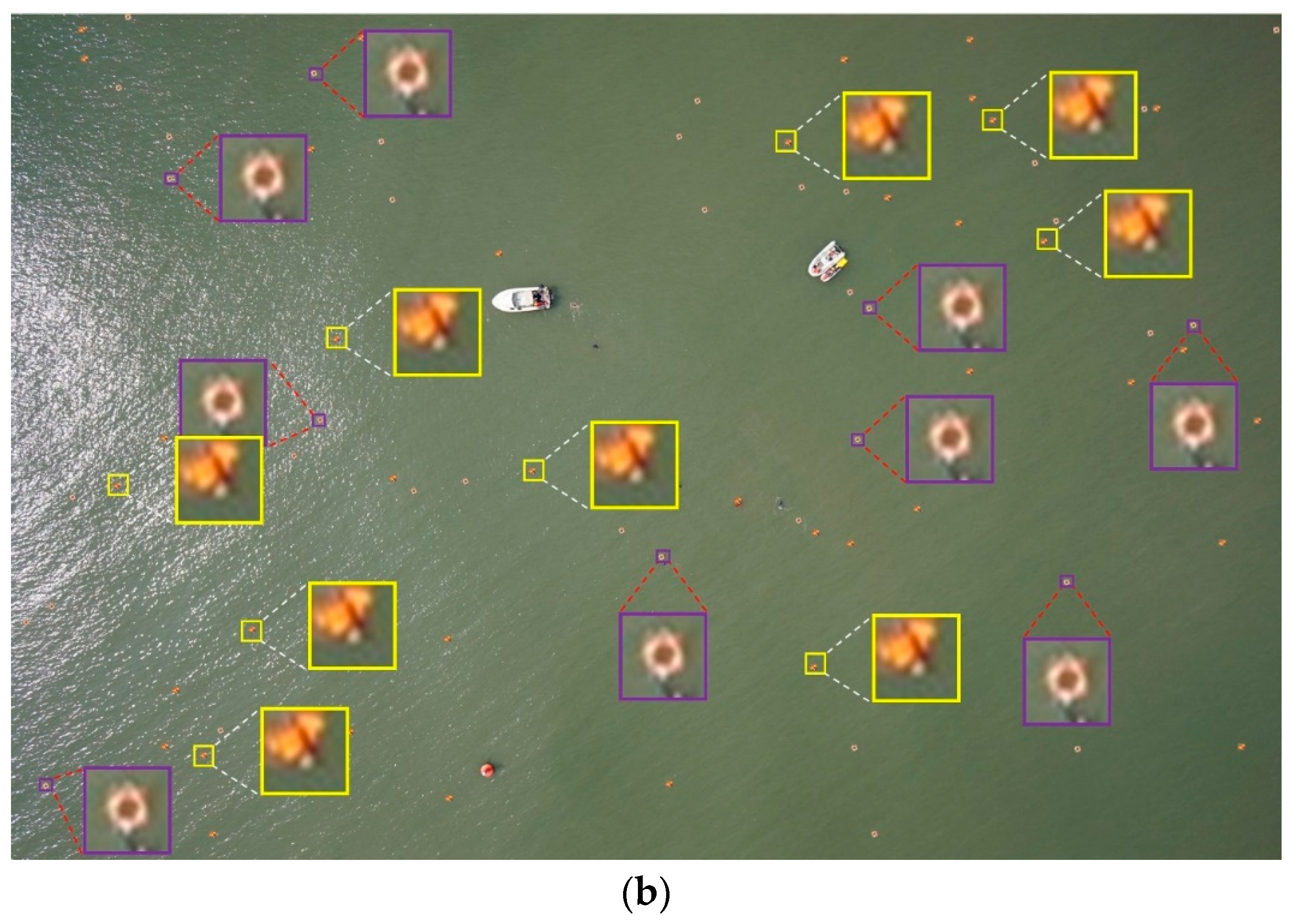
Class	Algorithms	P (%)	R (%)	mAP50val (%)	mAP50-95val (%)	Params (M)	FLOPs (G)	Speed RTX4090 b16 (ms)
1	YOLOv8s	80.2	59.9	66.1	39.9	11.14	28.7	2.6
2	a	84.1	62.2	67.7	40.2	11.14	28.7	2.6
3	b	79.8	60.5	66.6	39.9	9.59	25.7	1.2
4	c	82.8	59.5	66.5	39.3	9.48	23.8	1.4
5	d	86.8	70.5	76.7	42.7	6.86	31.1	2.4
6	b + c	81	59.4	66.1	39.0	7.93	20.9	1.1
7	b + c + d	82.6	71.3	76.6	43.5	3.65	23.3	2.1
8	a + b + c + d (our)	85.5	71.6	78.3	43.7	3.64	22.9	2.1

.

Table 9. The mAP50 results of ablation experiments for five categories on the SeaDroneSee-val.

Class	Algorithms	Swimmer	Boat	Jetski	Life_Saving_Appliances	Buoy	mAP50val (%)
1	YOLOv8s	69.6	91.6	83.7	28.2	57.2	66.1
2	a	66.0	91.2	84.6	35.4	61.4	67.7
3	b	69.4	91.1	85.6	30.7	56.1	66.6
4	c	70.4	91.7	81.4	28.7	60.2	66.5
5	d	77.6	95.6	87.4	45.5	77.2	76.7
6	b + c	69.8	90.5	82.4	27.6	60.1	66.1
7	b + c + d	78.3	95.5	86.3	45.8	77.3	76.6
8	a + b+c + d (our)	79.6	95.5	85.9	54.8	75.7	78.3

presents the mAP results of ablation experiments for five categories on the SeaDroneSee validation set. Figure 11 compares the mAP curves of eight sets of experimental results, and Figure 12 shows the scatter plot of model parameters and inference time for the eight sets of experiments. Since the previous sections have thoroughly analyzed the experimental results of each individual improvement, this chapter focuses on discussing and analyzing the combined impact of multiple improvements on the baseline model.

1. Lightweight improvements to the backbone network: From the results of Group 6 experiments in Table 8, we can see that compared with the baseline model, using DSConv and FC-C2f for lightweight improvements to the baseline model’s backbone network significantly reduces the model parameters and FLOPs while substantially increasing detection speed. Specifically, the model parameters decreased from 11.14 to 7.93, FLOPs reduced from 28.7 to 20.9, and detection time per image dropped from 2.6 ms to 1.1 ms. In addition, the change in detection accuracy before and after the lightweight improvements was minimal. Comparing Group 1 and Group 6 in Table 9, the Map metrics for the five categories show minimal change, demonstrating that the DSConv and FC-C2f modules can reduce computational redundancy and increase detection speed without affecting detection accuracy. Figure 11 and Figure 12 visually confirm these findings, showing that the lightweight improved model has similar Map curves to the YOLOv8s model but with fewer parameters and shorter inference time. The experiments demonstrate that DSConv and FC-C2f can improve the computational efficiency and reduce the complexity of the model without affecting detection accuracy.

2. LMFN: Comparing the experiments from Group 6 and Group 7, we can see that the proposed LMFN can enhance the model’s Precision, Recall, and Map, while reducing the model’s parameters. However, LMFN increases the model’s FLOPs due to its gradual fusion of multiple feature maps from different layers. This extensive cross-layer fusion mitigates information discrepancy between different feature levels, enhancing the model’s ability to recognize objects at various scales. However, this complex fusion process also leads to an increase in the model’s FLOPs and network delay. Comparing Group 6 and Group 7 in Table 9, the detection accuracy for all categories has improved. Additionally, we found that the extent of accuracy improvement is related to the size of the objects. The “life_saving_appliances” category, which contains the smallest objects, saw the greatest improvement of approximately 18.2%. In contrast, the “boat” category, with the largest objects, experienced the smallest improvement of about 5%. Thus, the LMFN can enhance the model’s detection performance for small objects through its multiscale fusion capability and ability to achieve a larger effective receptive field. Figure 11 and Figure 12 show that the Map curve of the LMFN-improved model is higher than that of the baseline model, although the inference time is increased. The experiments demonstrate that the LMFN proposed in this paper can effectively improve the detection accuracy of the model and reduce model parameters. Although the FLOPs increased from 20.9 to 23.3, this increase is negligible compared to the significant improvement in detection accuracy.

3. DFLM-YOLO: Comparing Group 8 of the experiments with the baseline model, we find that the proposed model improves precision by 6.4%, recall by 11.1%, and Map50 by 12.4%. The model parameters are reduced from 11.17 to 3.65, a reduction of 67.2%, and FLOPs decreases from 28.7 to 23.3, a reduction of 18.8%. Inference time is reduced from 2.6 ms to 2.3 ms, a reduction of 11.5%. Comparing Group 1 and Group 8 in Table 9, it is evident that the proposed DFLM-YOLO significantly improves detection accuracy for each category compared to YOLOv8s, with the most notable increases seen in the smaller-sized “life_saving_appliances” and “swimmer” categories. Figure 11 and Figure 12 demonstrate that DFLM-YOLO has the highest Map curve compared to other models, showing excellent detection accuracy while meeting real-time requirements. This model achieves a balance between detection accuracy and speed.

The experimental results show that the four proposed improvements to the baseline model not only improve detection accuracy but also achieve a lightweight design, simplifying the network structure, enhancing computational efficiency, and reducing network latency. These improvements ensure that the model meets the real-time and accuracy requirements for drone-based maritime object detection tasks.

Figure 13 shows the detection results of the DFLM-YOLO and YOLOv8s models in various maritime environments (with certain small areas enlarged). Figure 13a,b display detection scenarios in dense small-object environments. YOLOv8s misses some small objects, while DFLM-YOLO correctly identifies all small objects. Comparing the detection results in Figure 13c,d, DFLM-YOLO not only has a higher accuracy than YOLOv8s but also detects more small objects. The detection results in Figure 13e,f show that YOLOv8s mistakenly identifies “life-saving equipment” as “swimmers” due to their similar pixel characteristics, whereas the improved model correctly identifies the “life-saving equipment”. The detection results in Figure 13g,h indicate that DFLM-YOLO has a significantly higher detection accuracy and recall rate for small objects compared to YOLOv8s. Therefore, the proposed DFLM-YOLO algorithm outperforms the baseline model in small-object detection performance, providing a new solution for maritime object detection.

4.4. Comparative Experiment

To further validate the performance advantages of the DFLM-YOLO algorithm for small object detection with UAVs, comparative experiments are conducted against seven popular detection algorithms: YOLOv5s, YOLO-OW, YOLOv8n, YOLOv9t, YOLOv10s, YOLO-OW, and RT-DETR. Among these, YOLO-OW is the top-ranking detection model on the official leaderboard [49]. The experimental results of each model are shown in

Table 10. The influence of different models evaluated on SeaDroneSee-val.

Class	Algorithms	P (%)	R (%)	mAP50val (%)	mAP50-95val (%)	Params (M)	FLOPs (G)	Speed RTX4090 b16 (ms)
1	YOLOv5s	82.7	57.9	65.4	38.6	9.11	23.8	2.1
2	YOLOv6n	79.5	57.7	60.6	35.9	4.23	11.8	1.7
3	YOLOv8n	79.0	58.8	63.6	37.1	3.0	8.1	1.6
4	YOLOv9t	74.1	58.5	62.3	37.8	2.62	10.7	4.5
5	YOLOv10s	82.3	59.3	63.8	37.7	8.04	24.5	1.0
6	YOLO-OW	83.1	75.5	75.5	39.9	42.1	94.8	4.6
7	RT-DETR-R18	88.4	82.6	83.6	49.6	20.0	57.0	3.8
8	DFLM-YOLO (our)	85.5	71.6	78.3	43.7	3.64	22.9	2.1

.

According to Table 10, the proposed DFLM-YOLO algorithm significantly outperforms other algorithms with similar parameter levels in terms of detection accuracy. The parameter counts of YOLOv6n, YOLOv8n, and YOLOv9t are similar to that of the DFLM-YOLO algorithm, but the mAP scores of the DFLM-YOLO algorithm are higher by 17.7%, 14.7%, and 16%, respectively. As shown in

Table 11. The mAP results of comparative experiments for the five categories on the SeaDroneSee-val.

Class	Algorithms	Swimmer	Boat	Jetski	Life_Saving_Appliances	Buoy	mAP50val (%)
1	YOLOv5s	69.9	91.6	81.1	26.0	58.5	65.4
2	YOLOv6n	65.4	90.7	78.6	14.2	54.1	60.6
3	YOLOv8n	66.7	92.0	83.9	19.8	55.6	63.6
4	YOLOv9t	68.5	91.5	84.5	14.3	52.7	62.3
5	YOLOv10s	67.5	90.1	86.0	23.6	51.9	63.8
6	YOLO-OW	67.9	92.0	93.0	49.8	74.8	75.5
7	RT-DETR-R18	82.2	97.8	92.3	54.6	90.9	83.6
8	DFLM-YOLO (our)	79.6	95.5	85.9	54.8	75.7	78.3

, the detection accuracy of DFLM-YOLO is significantly higher across all categories compared to YOLOv6n, YOLOv8n, and YOLOv9t. The most notable improvement is in the “life_saving_appliances” category, where the accuracy is more than double that of the other models. The mAP curve in Figure 14 indicates that the DFLM-YOLO algorithm outperforms the other three algorithms. Figure 15 illustrates that YOLOv6n and YOLOv8n have inference times 0.4 ms and 0.5 ms faster than DFLM-YOLO, respectively, while YOLOv9t has an inference time of 4.5 ms, due to the auxiliary reversible branches used.

YOLOv5s and YOLOv10s have FLOPs similar to DFLM-YOLO, but their parameter counts are 2.5 times and 2.2 times higher, respectively, and their mAP scores are 12.9% and 14.5% lower than DFLM-YOLO. Additionally, DFLM-YOLO shows higher detection accuracy across all categories compared to YOLOv5s and YOLOv10s. As shown in Figure 15, YOLOv5s has a similar inference time to DFLM-YOLO, while YOLOv10s has an inference time of only 1 ms. This is because YOLOv10s uses a non-NMS training continuous dual assignment strategy, which significantly reduces inference time.

The mAP of the YOLO-OW algorithm is 73.1%, which is 5.2% lower than DFLM-YOLO. Its parameter count is 11.5 times that of DFLM-YOLO, its FLOPs is 4.1 times higher, and its inference time is as high as 4.5 ms. In repeated experiments under the same conditions, we observed that the mAP metric for YOLO-OW did not improve during the early stages of training. In repeated experiments under the same conditions, we observed that the mAP metric for YOLO-OW did not improve during the early stages of training. The mAP of RT-DETR-R18 is 5.3% higher than DFLM-YOLO, but its parameter count is 5.5 times higher, its FLOPs are 2.5 times greater, and its inference time is approximately twice that of DFLM-YOLO.

In summary, the DFLM-YOLO algorithm proposed in this paper demonstrates significant advantages in detection accuracy compared to current mainstream object detection algorithms, with similar parameter levels and FLOPs. The DFLM-YOLO maintains a low parameter count and FLOPs while meeting the requirements for high detection accuracy and real-time performance, providing a new solution for object detection in open water.

5. Conclusions

Object detection in open water is crucial for maritime rescue, resource management, and navigation. In this paper, we propose a lightweight object detection algorithm based on multiscale fusion, which improves the detection accuracy while satisfying the deployment conditions and real-time requirements of an airborne computation device.

This paper proposes a new data augmentation algorithm called SOM to address the class imbalance problem in the SeaDroneSee dataset. The algorithm increases the number of specified class objects through copy-paste without adding actual objects, thereby resolving the class imbalance problem. To meet the requirements of deploying an airborne computation device while maintaining the detection accuracy, firstly, we make the backbone of the original YOLOv8s network lightweight, introducing the lightweight feature extraction module FC-C2f, which significantly reduces model parameters and FLOPs, thereby shortening inference time. Additionally, DSConv was used to replace standard convolutions in the original network, further reducing the parameters and FLOPs of the backbone network. Finally, a lightweight multiscale feature fusion network, LMFN, was proposed as the neck network. The LMFN effectively reduces the contradiction between different feature layers by gradually fusing multiple feature layers extracted from the backbone network and improves the model’s ability to recognize multiscale objects. This paper introduces the DRB module into LMFN, which uses a re-parameterize module to equate multiple small kernel dilated convolutions to a single large kernel non-dilated convolution. The re-parameterize module consists of one non-dilated small convolution kernel and several dilated small convolution kernels. Research shows that the DRB module can significantly increase the effective receptive field of LMFN, enhancing the model’s detection performance, and improving the recall rate for small objects. However, while LMFN improves detection accuracy and reduces parameter count, the extensive fusion between the different feature layers increases the model’s complexity.

Although the proposed DFLM-YOLO model achieved good detection performance on the SeaDroneSee dataset, real sea conditions are far more complex than those represented in the dataset. Therefore, in future research, we will collect image data under extreme weather conditions and low-light environments (such as nighttime) to enhance the model’s adaptability and generalization in practical applications. Additionally, the DFLM-YOLO model has not addressed the adverse effects of sea surface glare and waves on small object detection. We will tackle this issue by improving network structure, feature fusion strategies, and exploring other data augmentation methods. In our subsequent research, we will also employ model compression techniques such as pruning and distillation to further reduce the model’s computational and parameter requirements. Furthermore, we will use hardware acceleration algorithms like TensorRT to deploy the model on airborne computing platforms.

References

- Yang, T.; Jiang, Z.; Sun, R.; Cheng, N.; Feng, H. Maritime Search and Rescue Based on Group Mobile Computing for Unmanned Aerial Vehicles and Unmanned Surface Vehicles. IEEE Trans. Ind. Inform. 2020, 16, 7700–7708. [Google Scholar] [CrossRef]
- Tang, G.; Ni, J.; Zhao, Y.; Gu, Y.; Cao, W. A Survey of Object Detection for UAVs Based on Deep Learning. Remote Sens. 2024, 16, 149. [Google Scholar] [CrossRef]
- Bouguettaya, A.; Zarzour, H.; Kechida, A.; Taberkit, A.M. Deep Learning Techniques to Classify Agricultural Crops through UAV Imagery: A Review. Neural Comput. Appl. 2022, 34, 9511–9536. [Google Scholar] [CrossRef]
- Zhao, C.; Liu, R.W.; Qu, J.; Gao, R. Deep Learning-Based Object Detection in Maritime Unmanned Aerial Vehicle Imagery: Review and Experimental Comparisons. Eng. Appl. Artif. Intell. 2024, 128, 107513. [Google Scholar] [CrossRef]
- Guo, Y.; Xiao, Y.; Hao, F.; Zhang, X.; Chen, J.; de Beurs, K.; He, Y.; Fu, Y.H. Comparison of Different Machine Learning Algorithms for Predicting Maize Grain Yield Using UAV-Based Hyperspectral Images. Int. J. Appl. Earth Obs. Geoinf. 2023, 124, 103528. [Google Scholar] [CrossRef]
- Yang, Z.; Yin, Y.; Jing, Q.; Shao, Z. A High-Precision Detection Model of Small Objects in Maritime UAV Perspective Based on Improved YOLOv5. J. Mar. Sci. Eng. 2023, 11, 1680. [Google Scholar] [CrossRef]
- Lin, T.-Y.; Maire, M.; Belongie, S.; Hays, J.; Perona, P.; Ramanan, D.; Dollár, P.; Zitnick, C.L. Microsoft COCO: Common Objects in Context. In Computer Vision—ECCV 2014, Proceedings of the 13th European Conference, Zurich, Switzerland, 6–12 September 2014; Proceedings, Part V 13; Springer: Cham, Switzerland, 2014; pp. 740–755. [Google Scholar]
- Ma, L.; Liu, Y.; Zhang, X.; Ye, Y.; Yin, G.; Johnson, B.A. Deep Learning in Remote Sensing Applications: A Meta-Analysis and Review. ISPRS J. Photogramm. Remote Sens. 2019, 152, 166–177. [Google Scholar] [CrossRef]
- Zhu, X.X.; Tuia, D.; Mou, L.; Xia, G.-S.; Zhang, L.; Xu, F.; Fraundorfer, F. Deep Learning in Remote Sensing: A Comprehensive Review and List of Resources. IEEE Geosci. Remote Sens. Mag. 2017, 5, 8–36. [Google Scholar] [CrossRef]
- Redmon, J.; Divvala, S.; Girshick, R.; Farhadi, A. You Only Look Once: Unified, Real-Time Object Detection. arXiv 2016, arXiv:1506.02640. [Google Scholar]
- Redmon, J.; Farhadi, A. YOLO9000: Better, Faster, Stronger. arXiv 2016, arXiv:1612.08242. [Google Scholar]
- Redmon, J.; Farhadi, A. YOLOv3: An Incremental Improvement. arXiv 2018, arXiv:1804.02767. [Google Scholar]
- Bochkovskiy, A.; Wang, C.-Y.; Liao, H.-Y.M. YOLOv4: Optimal Speed and Accuracy of Object Detection. arXiv 2020, arXiv:2004.10934. [Google Scholar]
- Jocher, G. YOLOv5 by Ultralytics. Available online: https://github.com/ultralytics/yolov5 (accessed on 1 May 2024).
- Li, C.; Li, L.; Jiang, H.; Weng, K.; Geng, Y.; Li, L.; Ke, Z.; Li, Q.; Cheng, M.; Nie, W.; et al. YOLOv6: A Single-Stage Object Detection Framework for Industrial Applications. arXiv 2022, arXiv:2209.02976. [Google Scholar]
- Wang, C.-Y.; Bochkovskiy, A.; Liao, H.-Y.M. YOLOv7: Trainable Bag-of-Freebies Sets New State-of-the-Art for Real-Time Object Detectors. arXiv 2022. [Google Scholar] [CrossRef]
- Varghese, R.; M., S. YOLOv8: A Novel Object Detection Algorithm with Enhanced Performance and Robustness. In Proceedings of the 2024 International Conference on Advances in Data Engineering and Intelligent Computing Systems (ADICS), Chennai, India, 18–19 April 2024; pp. 1–6. [Google Scholar]
- Wang, C.-Y.; Yeh, I.-H.; Liao, H.-Y.M. YOLOv9: Learning What You Want to Learn Using Programmable Gradient Information. arXiv 2024, arXiv:2402.13616. [Google Scholar]
- Wang, A.; Chen, H.; Liu, L.; Chen, K.; Lin, Z.; Han, J.; Ding, G. YOLOv10: Real-Time End-to-End Object Detection. arXiv 2024, arXiv:2405.14458. [Google Scholar]
- Chen, G.; Pei, G.; Tang, Y.; Chen, T.; Tang, Z. A Novel Multi-Sample Data Augmentation Method for Oriented Object Detection in Remote Sensing Images. In Proceedings of the 2022 IEEE 24th International Workshop on Multimedia Signal Processing (MMSP), Shanghai, China, 26–28 September 2022; pp. 1–7. [Google Scholar]
- Zhang, Q.; Meng, Z.; Zhao, Z.; Su, F. GSLD: A Global Scanner with Local Discriminator Network for Fast Detection of Sparse Plasma Cell in Immunohistochemistry. In Proceedings of the 2021 IEEE International Conference on Image Processing (ICIP), Anchorage, AK, USA, 19–22 September 2021; pp. 86–90. [Google Scholar]
- Ghiasi, G.; Cui, Y.; Srinivas, A.; Qian, R.; Lin, T.-Y.; Cubuk, E.D.; Le, Q.V.; Zoph, B. Simple Copy-Paste Is a Strong Data Augmentation Method for Instance Segmentation. In Proceedings of the 2021 IEEE/CVF Conference on Computer Vision and Pattern Recognition (CVPR), Nashville, TN, USA, 20–25 June 2021. [Google Scholar]
- Iandola, F.N.; Han, S.; Moskewicz, M.W.; Ashraf, K.; Dally, W.J.; Keutzer, K. SqueezeNet: AlexNet-Level Accuracy with 50× Fewer Parameters and <0.5 MB Model Size. arXiv 2016, arXiv:1602.07360. [Google Scholar]
- Howard, A.G.; Zhu, M.; Chen, B.; Kalenichenko, D.; Wang, W.; Weyand, T.; Andreetto, M.; Adam, H. MobileNets: Efficient Convolutional Neural Networks for Mobile Vision Applications. arXiv 2017, arXiv:1704.04861. [Google Scholar]
- Gholami, A.; Kwon, K.; Wu, B.; Tai, Z.; Yue, X.; Jin, P.; Zhao, S.; Keutzer, K. SqueezeNext: Hardware-Aware Neural Network Design. In Proceedings of the 2018 IEEE/CVF Conference on Computer Vision and Pattern Recognition Workshops (CVPRW), Salt Lake City, UT, USA, 18–22 June 2018. [Google Scholar]
- Sandler, M.; Howard, A.; Zhu, M.; Zhmoginov, A.; Chen, L.-C. MobileNetV2: Inverted Residuals and Linear Bottlenecks. In Proceedings of the 2018 IEEE/CVF Conference on Computer Vision and Pattern Recognition, Salt Lake City, UT, USA, 18–23 June 2018. [Google Scholar]
- Qin, D.; Leichner, C.; Delakis, M.; Fornoni, M.; Luo, S.; Yang, F.; Wang, W.; Banbury, C.; Ye, C.; Akin, B.; et al. MobileNetV4—Universal Models for the Mobile Ecosystem. arXiv 2024, arXiv:2404.10518. [Google Scholar]
- Howard, A.; Sandler, M.; Chu, G.; Chen, L.-C.; Chen, B.; Tan, M.; Wang, W.; Zhu, Y.; Pang, R.; Vasudevan, V.; et al. Searching for MobileNetV3. In Proceedings of the 2019 IEEE/CVF International Conference on Computer Vision (ICCV), Seoul, Republic of Korea, 27 October–2 November 2019. [Google Scholar]
- Zhang, J.; Chen, Z.; Yan, G.; Wang, Y.; Hu, B. Faster and Lightweight: An Improved YOLOv5 Object Detector for Remote Sensing Images. Remote Sens. 2023, 15, 4974. [Google Scholar] [CrossRef]
- Gong, W. Lightweight Object Detection: A Study Based on YOLOv7 Integrated with ShuffleNetv2 and Vision Transformer. arXiv 2024, arXiv:2403.01736. [Google Scholar]
- Wang, J.; Chen, K.; Xu, R.; Liu, Z.; Loy, C.C.; Lin, D. CARAFE: Content-Aware ReAssembly of FEatures. In Proceedings of the 2019 IEEE/CVF International Conference on Computer Vision (ICCV), Seoul, Republic of Korea, 27 October–2 November 2019; pp. 3007–3016. [Google Scholar]
- Lin, T.-Y.; Dollár, P.; Girshick, R.; He, K.; Hariharan, B.; Belongie, S. Feature Pyramid Networks for Object Detection. In Proceedings of the IEEE Conference on Computer Vision and Pattern Recognition, Honolulu, HI, USA, 21–26 July 2017. [Google Scholar]
- Liu, S.; Qi, L.; Qin, H.; Shi, J.; Jia, J. Path Aggregation Network for Instance Segmentation. In Proceedings of the 2018 IEEE/CVF Conference on Computer Vision and Pattern Recognition, Salt Lake City, UT, USA, 18–23 June 2018; pp. 8759–8768. [Google Scholar]
- Xu, X.; Jiang, Y.; Chen, W.; Huang, Y.; Zhang, Y.; Sun, X. DAMO-YOLO: A Report on Real-Time Object Detection Design. arXiv 2023, arXiv:2211.15444. [Google Scholar]
- Tan, M.; Pang, R.; Le, Q.V. EfficientDet: Scalable and Efficient Object Detection. In Proceedings of the IEEE/CVF Conference on Computer Vision and Pattern Recognition, Seattle, WA, USA, 13–19 June 2020. [Google Scholar]
- Li, K.; Geng, Q.; Wan, M.; Cao, X.; Zhou, Z. Context and Spatial Feature Calibration for Real-Time Semantic Segmentation. IEEE Trans. Image Process. 2023, 32, 5465–5477. [Google Scholar] [CrossRef]
- Kisantal, M.; Wojna, Z.; Murawski, J.; Naruniec, J.; Cho, K. Augmentation for Small Object Detection. arXiv 2019, arXiv:1902.07296. [Google Scholar]
- Guo, Y.; Li, Y.; Feris, R.; Wang, L.; Rosing, T. Depthwise Convolution Is All You Need for Learning Multiple Visual Domains. Available online: https://arxiv.org/abs/1902.00927v2 (accessed on 16 May 2024).
- Chen, J.; Kao, S.; He, H.; Zhuo, W.; Wen, S.; Lee, C.-H.; Chan, S.-H.G. Run, Don’t Walk: Chasing Higher FLOPS for Faster Neural Networks. arXiv 2023, arXiv:2303.03667. [Google Scholar]
- Ma, N.; Zhang, X.; Zheng, H.-T.; Sun, J. ShuffleNet V2: Practical Guidelines for Efficient CNN Architecture Design. In Computer Vision—ECCV 2018; Ferrari, V., Hebert, M., Sminchisescu, C., Weiss, Y., Eds.; Springer International Publishing: Cham, Switzerland, 2018; pp. 122–138. [Google Scholar]
- Han, K.; Wang, Y.; Tian, Q.; Guo, J.; Xu, C.; Xu, C. GhostNet: More Features from Cheap Operations. In Proceedings of the 2020 IEEE/CVF Conference on Computer Vision and Pattern Recognition (CVPR), Seattle, WA, USA, 13–19 June 2020; pp. 1577–1586. [Google Scholar]
- Zhao, Y.; Lv, W.; Xu, S.; Wei, J.; Wang, G.; Dang, Q.; Liu, Y.; Chen, J. DETRs Beat YOLOs on Real-Time Object Detection. arXiv 2024, arXiv:2304.08069v3. [Google Scholar]
- Dauphin, Y.N.; Fan, A.; Auli, M.; Grangier, D. Language Modeling with Gated Convolutional Networks. PMLR 2017, 70, 933–941. [Google Scholar]
- Shi, D. TransNeXt: Robust Foveal Visual Perception for Vision Transformers. arXiv 2024, arXiv:2311.17132. [Google Scholar]
- Yang, G.; Lei, J.; Zhu, Z.; Cheng, S.; Feng, Z.; Liang, R. AFPN: Asymptotic Feature Pyramid Network for Object Detection. In Proceedings of the 2023 IEEE International Conference on Systems, Man, and Cybernetics (SMC), Honolulu, HI, USA, 1–4 October 2023. [Google Scholar]
- Ding, X.; Zhang, X.; Zhou, Y.; Han, J.; Ding, G.; Sun, J. Scaling Up Your Kernels to 31 × 31: Revisiting Large Kernel Design in CNNs. arXiv 2022, arXiv:2203.06717. [Google Scholar]
- Luo, W.; Li, Y.; Urtasun, R.; Zemel, R. Understanding the Effective Receptive Field in Deep Convolutional Neural Networks. arXiv 2017, arXiv:1701.04128. [Google Scholar]
- Ding, X.; Zhang, Y.; Ge, Y.; Zhao, S.; Song, L.; Yue, X.; Shan, Y. UniRepLKNet: A Universal Perception Large-Kernel ConvNet for Audio, Video, Point Cloud, Time-Series and Image Recognition. arXiv 2024, arXiv:2311.15599. [Google Scholar]
- Xu, J.; Fan, X.; Jian, H.; Xu, C.; Bei, W.; Ge, Q.; Zhao, T. YoloOW: A Spatial Scale Adaptive Real-Time Object Detection Neural Network for Open Water Search and Rescue From UAV Aerial Imagery. IEEE Trans. Geosci. Remote Sens. 2024, 62, 5623115. [Google Scholar] [CrossRef]