Risk Assessment and Distribution Estimation for UAV Operations with Accurate Ground Feature Extraction Based on a Multi-Layer Method in Urban Areas

Abstract

In this paper, a quantitative ground risk assessment mechanism is proposed in which urban ground features are extracted based on high-resolution data in a satellite image when unmanned aerial vehicles (UAVs) operate in urban areas. Ground risk distributions are estimated and a risk map is constructed with a multi-layer method considering the comprehensive risk imposed by UAV operations. The urban ground feature extraction is first implemented by employing a K-Means clustering method to an actual satellite image. Five main categories of the ground features are classified, each of which is composed of several sub-categories. Three more layers are then obtained, which are a population density layer, a sheltering factor layer, and a ground obstacle layer. As a result, a three-dimensional (3D) risk map is formed with a high resolution of 1 m × 1 m × 5 m. For each unit in this risk map, three kinds of risk imposed by UAV operations are taken into account and calculated, which include the risk to pedestrians, risk to ground vehicles, and risk to ground properties. This paper also develops a method of the resolution conversion to accommodate different UAV operation requirements. Case study results indicate that the risk levels between the fifth and tenth layers of the generated 3D risk map are relatively low, making these altitudes quite suitable for UAV operations.

1. Introduction

In recent years, unmanned aerial vehicles (UAVs) have become the fastest growing sector in aviation, and have been widely used in many fields, such as agriculture, infrastructure management, logistics, emergency response, and scientific research [1,2,3]. Concerns have been raised regarding the potential risk that is posed by UAV operations. IN particular, a great number of UAVs are expected to operate at low altitude in urban airspace. In this regard, ensuring flight safety is quite critical to the mission capability and security of UAVs, and there is thus an increasing need to develop and improve the technique of risk assessment for UAVs [4].

However, a comprehensive understanding of the UAV operation risk in urban areas has yet to be fully attained. To conduct the risk assessments for UAV operations, the Joint Authorities for Rulemaking on Unmanned Systems (JARUS) have issued a guidance document that is known as Specific Operational Risk Assessment (SORA), which is a foundation for UAV operational risk testing [5]. SORA breaks down a complex risk assessment step by step and takes a qualitative approach to risk assessment. According to JARUS, however, this SORA methodology is still under development and does not describe the risk distribution in the mission airspace.

A lot of research has been conducted on designing risk assessment methods to provide a risk analysis for UAV operations. Mitici et al. [6] utilized a unified mathematical framework to summarize various mathematical models for estimating air traffic conflict and collision probability, providing insights for the next-generation design of Air Traffic Management (ATM). Kaya et al. [7] proposed a risk assessment algorithm using a probabilistic risk exposure map considering the risk to people and property on the ground. Shelley [8] established a UAV kinetic energy model to assess a ground risk mitigation. La Cour-Harbo [9] proposed a method based on a standard stochastic model and a parametric high-fidelity ground impact distribution model to quantify the probability of fatalities due to UAVs’ uncontrolled descent. Liu et al. [10] analyzed the random uncertainties, such as the UAV speed and wind speed during the descent, to provide an accurate estimation of the UAV ground crash risk.

Determining how to construct a risk map describing the ground risk distributions based on the risk estimation is another crucial problem. First of all, defining and quantifying risk metrics are essential for developing a comprehensive risk map. The current research has focused on addressing some specific aspects of risk map representation, primarily considering ground risk with the population density and obstacles. Primatesta et al. [11,12] developed a location-based two-dimensional risk map quantifying the risk of UAV operation areas that integrates multiple factors. Pang and Hu [13,14] proposed an integrated cost assessment model for the three-dimensional UAV path planning problem, in which high-risk zones can be identified effectively and the risk cost of a planned UAV path can be mitigated. Su et al. [15] investigated a kinetic model and created a risk cost map based on the probabilistic impact of potential UAV collisions with pedestrians and ground vehicles. Schopferer et al. [16] analyzed the operation risk of UAVs based on semantic geospatial datasets and sample-based planning algorithms. Pilko et al. [17] assessed the ground risk due to UAV crashes with spatiotemporal population density data, which allowed for a dynamic assessment of the ground risk as well as improving the accuracy of the risk estimation. Sivakumar et al. [18] utilized public transportation data and applied a diffusive model to assess the risk caused by UAV operations.

With the development of artificial intelligence technology, several deep learning methods have been applied to the study of population density prediction based on spatiotemporal features to improve the accuracy and reliability of a risk assessment. Zhang et al. [19,20] proposed a method based on deep learning to predict population inflow and outflow in different urban regions, which can then be used to improve the availability of UAV risk estimation. Inspired by this, Jiao et al. [21] established a dynamic model to predict the ground risk combining deep learning and a kinetic model.

However, the resolution of a constructed risk map is currently not high enough and cannot define the ground risk distributions with an accepted accuracy. For example, the size of each cell in a risk map is normally 100 m × 100 m. In this situation, it is not suitable for a quite complicated urban area. As a result, the operations of UAVs in urban environments inevitably enter high-risk areas due to insufficient map accuracy.

This paper proposes a quantitative risk assessment method for extracting urban ground features based on high-resolution data in a satellite image to calculate the accurate risk of each grid. Furthermore, a ground risk map is generated using a multi-layer method to define the risk distributions that are caused by UAV operations in urban areas. This constructed risk map dynamically adjusts its size of each risk grid according to the actual urban scenarios. In the proposed method, a K-Means clustering method is imported to classify the actual urban satellite images at the pixel level, and five main categories of the ground features are obtained. Different risk sources from UAV operations are mapped to the ground grid and evaluated by an independent evaluation procedure. Three map layers are obtained, which are a population density layer, a sheltering factor layer, and a ground obstacle layer. As a result, a ground grid map is formed with a high resolution of 1 m × 1 m. For each cell in this grid map, two kinds of risk imposed by UAV operations are taken into account and calculated, which are the fatality risk cost and property damage cost.

The rest of the paper is structured as following. The problem description is given in Section 2. The extraction of urban ground features based on the high-resolution data in a satellite image, as well as the construction of the three map layers, are described in Section 3. The risk assessment model and generation of a risk map are proposed in Section 4. A case study and algorithm validations can be found in Section 5. Finally, the paper is concluded in Section 6.

2. Problem Description

Urban environments are characterized by a dense population, a lot of ground vehicles, high-rise buildings, and many critical infrastructures. UAVs operating in such urban airspace would encounter a great amount of risk issues [22]. In this way, two essential steps must be addressed in detail to accurately conduct a risk assessment. The first is to identify the third-party risk imposed by UAV operations and the other one is to quantify the identified risk accurately. Based on the analysis, the impacts of crashed UAVs on ground pedestrians, vehicles, and properties become the main focus.

In this paper, two main types of risk caused by UAV operations in urban areas are taken into account, which are the fatality risk and the property damage risk, as shown in Figure 1. The former includes the risk to ground pedestrians and risk to ground vehicles. Furthermore, a representative distribution of risk sources is given, which is not only in terms of a population distribution and the surface traffic, but also in terms of a complex combination of ground features that would affect the risk assessment. The definitions can be found below.

Fatality risk is defined as when the crashed UAV strikes pedestrians and vehicles on the ground, which would correspondingly result in fatalities. Property damage is defined as when the crashed UAV results in collisions with high-rise buildings or critical infrastructures, which causes the property damage.

According to the flying height where a UAV failure event happens, the urban airspace could be divided into many voxel grids based on an integrated cost model, each of which is defined as a cuboid with a centroid C_xyz. In this way, the urban airspace can be represented as a risk-based model, which is shown in Figure 2. In this paper, a risk map is defined as a three-dimensional location-based map that quantifies the risk in each cuboid.

A multi-layer method is used to construct a risk map, which is shown in Figure 3. Several map layers that affect the risk distributions are generated first, which include a population density layer, a sheltering factor layer, and a ground obstacle layer. In order to enhance the resolution of the generated risk map, a K-Means clustering method is applied to the actual urban satellite image at the pixel level for each layer separately, which results in a risk map that is more suitable for UAVs operating in urban environments. Note the collisions between UAVs themselves and between manned aircraft are not in the scope of this paper.

3. Methodology for Generating Map Layers

Based on the analysis above, several ground parameters should be obtained accurately when a layer-based method is used, which includes the population density, the sheltering factors, and the ground obstacle heights. The authentic satellite image and ground population are the two that are first imported and further classified to better calculate these needed parameters. Figure 4 shows how the multiple map layers are generated.

As shown in Figure 4, there are some types of data that should be given at the beginning, such as a satellite image, population data on the ground, and ground obstacle heights. Once the data are given, analysis and mining should be performed based on the satellite image and the population density in urban areas. The K-Means clustering method is used to obtain the ground features in each grid on the ground. A sheltering factor layer can then be formed. A correction coefficient is defined to accurately calculate the ground grid population, which then represents a population density layer. According to the obstacle heights on the ground, three main obstacle types are defined to denote a ground obstacle layer.

3.1. Classification of the Satellite Image

Regarding the current image classification techniques, it is possible to obtain a high-resolution risk layer based on a pixel-level feature classification of a satellite image, which greatly enables a refined analysis and assessment of the needed risk factors.

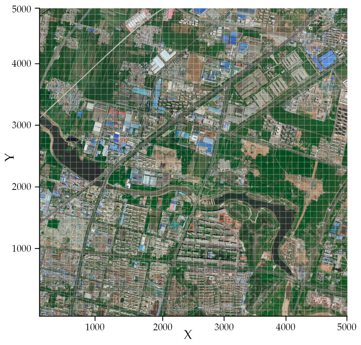
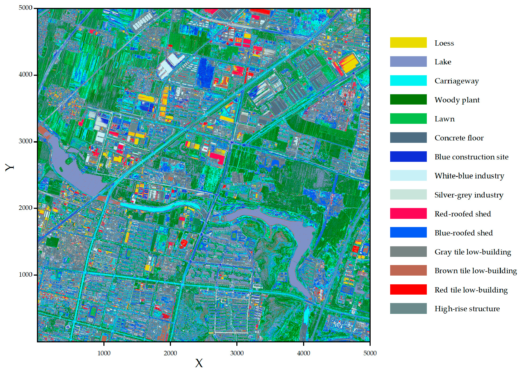
In this section, a satellite image of Changqing District in Jinan City is used, in which a sheltering factor layer is generated to further construct a risk-based airspace model. The satellite image was derived from Baidu Maps with a size of 5 km × 5 km. It means that all the UAVs would operate in this specified area. This selected area with a size of 5 km × 5 km is composed of many different ground features, such as high-rise buildings, industrial zones, and parks.

It is obvious that this obtained satellite image is composed of three channels of red, green, and blue (RGB), but with no label. In this situation, an unsupervised clustering method can be used to create a classification to extract the ground features. The K-Means clustering method [23] is the most well-known and commonly used approach for clustering problems, and it is also a type of unsupervised learning method. This algorithm partitions a whole dataset into K clusters according to the similarities between different samples. Data points would exhibit a significant similarity within the same cluster, while they would be marked as quite dissimilar if they are in different clusters.

There are three channels in a satellite image denoted as RGB, which are red, green, and blue. RGB indicates that each pixel in a satellite image possesses three features. For each channel in RGB, there are 256 brightness levels with values ranging from 0 to 255. There is also no need for data normalization. The size of a pixel in an actual map is set as 1 m × 1 m. The Euclidean distance is employed for calculating the distance from each pixel point to a cluster center, and this objective function can be expressed in Equation (1).

$$J={\displaystyle \sum _{i=1}^K{\displaystyle \sum _{j=1}^{C_i}\Vert p_{ij}-u_i\Vert }}$$

(1)

In Equation (1), K is the number of clusters, C_i is the number of pixel points in the ith cluster, p_ij denotes the jth data point in the ith cluster, and u_i signifies the center of mass of the ith cluster. In the K-Means clustering method, a cluster center u_i would be updated iteratively by minimizing the objective function J in Equation (1). The aim is to assign the data points to the nearest cluster center and then to optimize the clustering effects by adjusting the location of a cluster center.

Using the K-Means clustering method, the ground features are extracted and divided into five main categories, each of which is composed of several types. The total number of ground features is 15 after the extraction, as given in

Table 1. Classification of ground features.

No.	Ground Features
Category 1	Lawn, Lake, Concrete Floor, Loess, Blue Construction Site
Category 2	Carriageway
Category 3	Woody Plant, Blue-Roofed Shed, Red-Roofed Shed
Category 4	Tile Low Building (Brown, Gray, Red), Industrial Area (Silver-Grey, White-Blue)
Category 5	High-Rise Structure

.

As shown in Table 1, in Category 1 there are five types of ground features, which are Lawn, Lake, Concrete Floor, Loess, and Blue Construction Site. The Carriageway type belongs in Category 2. The Woody Plant, Blue-Roofed Shed, and Red-Roofed Shed are in the scope of Category 3. Tile Low Building (Brown, Gray, Red), and Industrial Area (Silver-Grey, White-Blue) are in Category 4. Category 5 is the High-Rise Structure.

Algorithm 1 shows the pseudocode of the K-Means clustering method. In this method, a pixel P and an initial clustering center U of all the pixels in a satellite image are defined as the input. Then the algorithm starts the iteration. Each data point is assigned to the nearest cluster center, and after that the position of the cluster center is updated according to all the data included in it. Each data point is assigned to the nearest cluster center. Following this assignment, the position of each cluster center is updated based on the mean of all data points assigned to that cluster. This iterative procedure continues until the cluster center remains unchanged. Finally, the clustering result C and the set of cluster centers U can be obtained.

Algorithm 1 K-Means clustering method
1:	Procedure K-Means (P, U)
2:	Let m = len(P), K = len(U)
3:	repeat
4:	Let Ci = Ø (1 ≤ i ≤ K)
5:	for j = 1, 2, …, m do
6:	Calculate distance: dji = ||pj − ui||2 (ui in U)
7:	Determine cluster label for pj: λj = argmini∈(1, 2, …, K) dji
8:	Add pj to C: Cλj = Cλj ∪ {pj}
9:	end for
10:	for i = 1, 2, …, K do
11:	Calculate new clustering center: u’i = ∑pij∈Ci pij/|Ci|
12:	if u’i ≠ ui then
13:	Update ui = u’i
14:	end if
15:	end for
16:	until centroids remain unchanged
17:	return (C, U)
18:	end Procedure

Furthermore, a similarity-matching process is required to identify the accurate types of ground features corresponding to the cluster center. In this paper, a total of 15 types of ground feature are considered and collected from a satellite image, and are represented as pixel points u’_i (i = 1, 2, …., 15). All of them are denoted as a ground feature set U’ = {u’₁, u’₂, …, u’₁₅}. The Euclidean distance is employed to calculate the distances between U and U’, which results in a similarity matrix D with a size of 15 × 15. U denotes the set of clustering centers obtained from applying the K-Means clustering algorithm to the satellite image. In this similarity matrix D, each element d_ij represents a Euclidean distance between the ith vector in U and the jth vector in U’. It is obvious that d_ij = ||u_i − u’_j||.

In order to determine the optimal clustering centers for different ground features, a similarity-matching problem is transformed into a task allocation problem by processing a similarity matrix D. The objective function is defined as given in Equation (2).

$$\begin{array}{l}\min Z={\displaystyle \sum _{i=1}^n{\displaystyle \sum _{j=1}^n{c}_{ij}{d}_{ij}}}\\ subject to \{\begin{array}{l}{\displaystyle \sum _{i=1}{c}_{ij}=1,j=1,2\dots ,n}\\ {\displaystyle \sum _{j=1}{c}_{ij}=1,i=1,2\dots ,n}\\ c_{ij}=1 or 0\end{array}\end{array}$$

(2)

In this equation, c_ij = 1 means the ith clustering center is matched to the jth ground feature. Otherwise, there would be no match and then n would be set as 15. In this way, each ground feature can find its optimal pixel center.

3.2. Modeling of a Population Density Layer

The population density layer defines ground population density and its distribution in specified urban areas, which is indispensable when the ground risk is assessed and estimated. Population density indicates the potential number of ground individuals that would be impacted by the crashed UAVs. Consequently, determining how to construct a population density layer with an accepted resolution based on the ground grid division becomes imperative.

3.2.1. Data Acquisition and Preprocessing

To generate a population density layer that is as accurate as possible, the population data were acquired from an open source of WorldPop (World Population) [24] and the official government data of the Seventh National Census Bulletin of Jinan City. WorldPop is a project that aims to provide a global population distribution and population density data. The population data of WorldPop are usually based on various information sources such, as the satellite remote sensing images, geographic statistics, and ground surveys, which greatly improves its accuracy and reliability. The Seventh National Census is a comprehensive census conducted by the Chinese government every ten years and issued to the public. It collects data on the basic population information, economic status, education level, living conditions, and other aspects.

The Chinese population distribution estimation dataset of the year 2020 was obtained from WorldPop. For this dataset, the Geographic Coordinate System WGS84 is used and the ground is divided into many grids. The resolution of the ground grid is 100 m × 100 m, and its unit is the number of people located in a ground grid. A random forest-based asymmetric redistribution is used as a mapping approach. The data of the census bulletin are straightforward, and the total number of people in Changqing District of Jinan in the year 2020 was obtained to further correct and refine the population data from WorldPop.

3.2.2. Estimation of Ground Population Density

In this paper, Changqing District in Jinan City is selected as the UAV operation scenario and the population data of Changqing District from the Chinese population distribution dataset are cropped first. Because of the potential delay in the WorldPop dataset, and aiming for a more accurate population density, a correction coefficient is proposed by incorporating the census data.

The correction coefficient (C_c) is defined in Equation (3), which represents a ratio of the census data of Changqing District (N_census) to the total population (N_WorldPop) of Changqing District estimated by WorldPop. Subsequently, to derive a more accurate population distribution of Changqing District, the population density in each ground grid is corrected by multiplying the proposed correction coefficient (C_c).

$$C_c={\displaystyle \frac{N_{census}}{N_{WorldPop}}}$$

(3)

Equation (4) shows the accurate calculation of the population density using the WorldPop population density in each ground grid and the proposed correction coefficient (C_c). ρ_correction is the corrected population density in a ground grid and ρ_people is the corresponding population density of a ground grid. Upon obtaining the corrected population density of Changqing District with Equation (4), it should be adjusted according to the dimension of the UAV operation areas. In this paper, all the UAVs are restricted within an area of 5 km × 5 km with a resolution of 100 m × 100 m. This means that the distribution of the corrected population density should follow this setting at the same time.

$${\rho }_{correction}={\rho }_{people}\cdot C_c$$

(4)

To obtain higher-resolution population density estimates, the classified ground features listed in Table 1 are considered. It is known that different ground features in a satellite image possess different population densities. However, the population density of the same ground feature in different locations would also be quite different. For example, a population density of a sidewalk near a shopping mall is definitely different from that of a sidewalk in a residential area. According to the analysis above, the total number of people on the ground in a specified urban area should be calculated first using Equation (5) based on different ground features.

$$N_p={\displaystyle \sum _{i=1}^k{A}_i{\rho }_i}$$

(5)

In Equation (5), N_p is the total number of people on the ground in a specified urban area. ρ_i is the population density of the i-th ground feature. A_i is the area of this corresponding i-th ground feature. In this paper, the resolution of the ground feature classification is defined as 1 m × 1 m, and the area of each ground feature can then be calculated easily. The initial grid size for a population density layer is 50 × 50. In this way, a total of 2500 linear equations can be established to calculate the number of people in a specified ground grid, as shown in Equation (6). 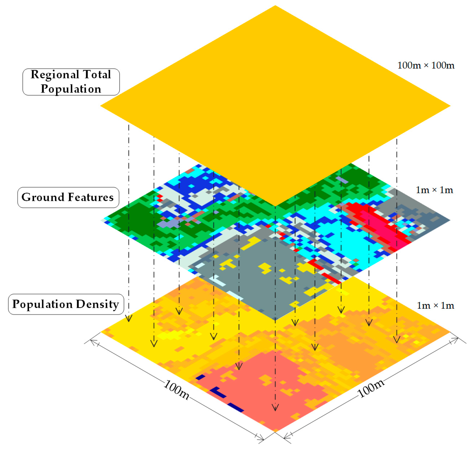Figure 5 illustrates how each equation calculates population density using ground feature classification and regional total population. Specifically, the top layer of the diagram represents the WorldPop data adjusted by a correction coefficient, yielding ρ_correction with a resolution of 100 m × 100 m. By calculating the area of each ground feature in the middle layer (with a resolution of 1 m × 1 m), the population density of each ground feature in the bottom layer can be determined. In the bottom layer of the figure, the color spectrum ranges from pale yellow to deep brown, where pale yellow indicates the lowest population density, and deep brown signifies the highest population density. This gradient provides a clear visual representation that different ground features have their corresponding population densities.

In Equation (6), A_n’k denotes the area of the kth ground feature given in Table 1 in the nth ground region and ρ_k is the population density of the kth ground feature. N_n is the total number of people in the nth ground region.

$$\{\begin{array}{l}{A}_{1^{\prime }1}{\rho }_1+A_{1^{\prime }2}{\rho }_2+\cdots +A_{1^{\prime }k}{\rho }_k=N_1\\ A_{2^{\prime }1}{\rho }_1+A_{2^{\prime }2}{\rho }_2+\cdots +A_{2^{\prime }k}{\rho }_k=N_2\\ ⋮⋮⋮\\ A_{n^{\prime }1}{\rho }_1+A_{n^{\prime }2}{\rho }_2+\cdots +A_{n^{\prime }k}{\rho }_k=N_n\end{array}$$

(6)

Because Equation (6) is a multiple linear regression model, it can be solved by a multiple linear regression method. However, it is also essential to emphasize that the key intercept term in this mentioned regression model should be 0.

Considering the fact that the population densities of the same type of ground feature may vary in different locations, the WorldPop data are used to correct the population densities of the same ground feature in different urban places. This step makes the obtained population density more accurate and reliable. To evaluate the contributions by incorporating these two kinds of data to a population density, a weight factor α_k is defined, and the final population density can be obtained with Equation (7).

$${\rho }_P={\alpha }_1{\rho }_1+{\alpha }_2{\rho }_2$$

(7)

In Equation (7), ρ_P is the final obtained population density. α_k denotes the kth weight factor and ρ_k is the kth population density. It should be noted that ρ₁ and ρ₂ correspond to the population densities of the ground features and WorldPop at a location, respectively. Here {α₁, α₂} ∈ (0, 1] and α₁ + α₂ = 1.

3.3. Modeling of a Sheltering Factor Layer

The sheltering factor is the level of protection that could be provided by buildings, structures, or trees to pedestrians in the event of a UAV crashing to the ground [25]. A sheltering factor is a positive number that reflects the degree of shielding effects, with higher values indicating a greater level of the provided protection. The sheltering factor is crucial as it mitigates the kinetic energy impact in the event of a UAV crash, thereby decreasing the fatality risk. Neglecting the sheltering factor leads to an assessment that fails to accurately represent the actual conditions, overlooking the protective shading effects of buildings, vehicles, and trees offered to ground people.

The precise concept of a sheltering factor has been defined differently across multiple studies, yet it can be generally classified into two categories. The first is that a sheltering factor is defined as a real number ranging from 0 to positive infinity, where 0 signifies the absence of any shelter with no protections and infinity denotes powerful protection. However, an excessively high value of the sheltering factor suffers from a lack of an evaluative significance. This is because substantial kinetic energy would be required to cause a fatality once it is beyond a certain threshold. Another approach is to confine the sheltering factor within a fixed range, ensuring that the assessment of the sheltering effect is more scientific and accurate.

In this section, a sheltering factor is defined based on the previous results of ground feature classifications. This means that the sheltering factors are assigned to the classified ground features with limited values. According to the classifications of ground features given in Table 1, the fifteen classified types of ground features are allocated with a fixed sheltering factor with a value between 0 and 1.

Table 2. Sheltering factors of ground features.

No.	Ground Features	Sheltering Factor
Category 1	Lawn, Lake, Concrete Floor, Loess, Blue Construction Site	0
Category 2	Carriageway	0.25
Category 3	Woody Plant, Blue-Roofed Shed, Red-Roofed Shed	0.50
Category 4	Tile Low Building (Brown, Gray, Red), Industrial Area (Silver-Grey, White-Blue)	0.75
Category 5	High-Rise Structure	1

gives the sheltering factors of different ground features. As shown in Table 2, the sheltering factors are set as 0, 0.25, 0.50, 0.75, and 1 for the five classified categories of ground features, respectively.

The sheltering factor of Lawn, Lake, Concrete Floor, Loess, and Blue Construction Site is 0, which means no protection can be provided when the UAVs crash into these areas. The Carriageway could provide protection with a sheltering factor 0.25. Woody Plant, Blue-Roofed Shed, and Red-Roofed Shed belong to the third category, whose sheltering factor is set as 0.5. Tile Low Building (Brown, Gray, Red), and Industrial Area (Silver-Grey, White-Blue) are in the scope of Category 4. Its sheltering factor is 0.75. Category 5 is High-Rise Structure, whose sheltering factor is the greatest, at 1.

Based on the above settings, for the ground feature classification results generated from the satellite image in Section 3.1, we assign the corresponding sheltering factor to obtain the sheltering factor layer. Similar to the ground feature classification, the resolution of this layer is also defined as 1 m × 1 m. This ensures that each 1 m × 1 m grid cell is assigned an appropriate sheltering factor, reflecting the level of protection provided by the ground feature in that grid.

3.4. Modeling of a Ground Obstacle Layer

In this section, the classified ground features given in Table 1 are taken into account to generated a ground obstacle layer. It is known that each type of ground feature has a specific height and can be treated as an obstacle in the urban airspace. In this way, all the UAVs are not permitted to fly within these occupied spaces or collide with them. Generally speaking, the denser the obstacles, the more risk for UAV operations in that area.

To generate a more accurate obstacle layer, all the ground obstacles are categorized into three main types by considering all the ground features given in Table 1 The first type consists of ground areas without high structures, such as grasslands or lakes, whose sheltering factor is generally zero. The second type includes trees, which are typically not as high in urban environments. The third type comprises urban buildings, which usually have a height of 4 m or more, and would significantly influence the UAV operation’s efficiency and safety.

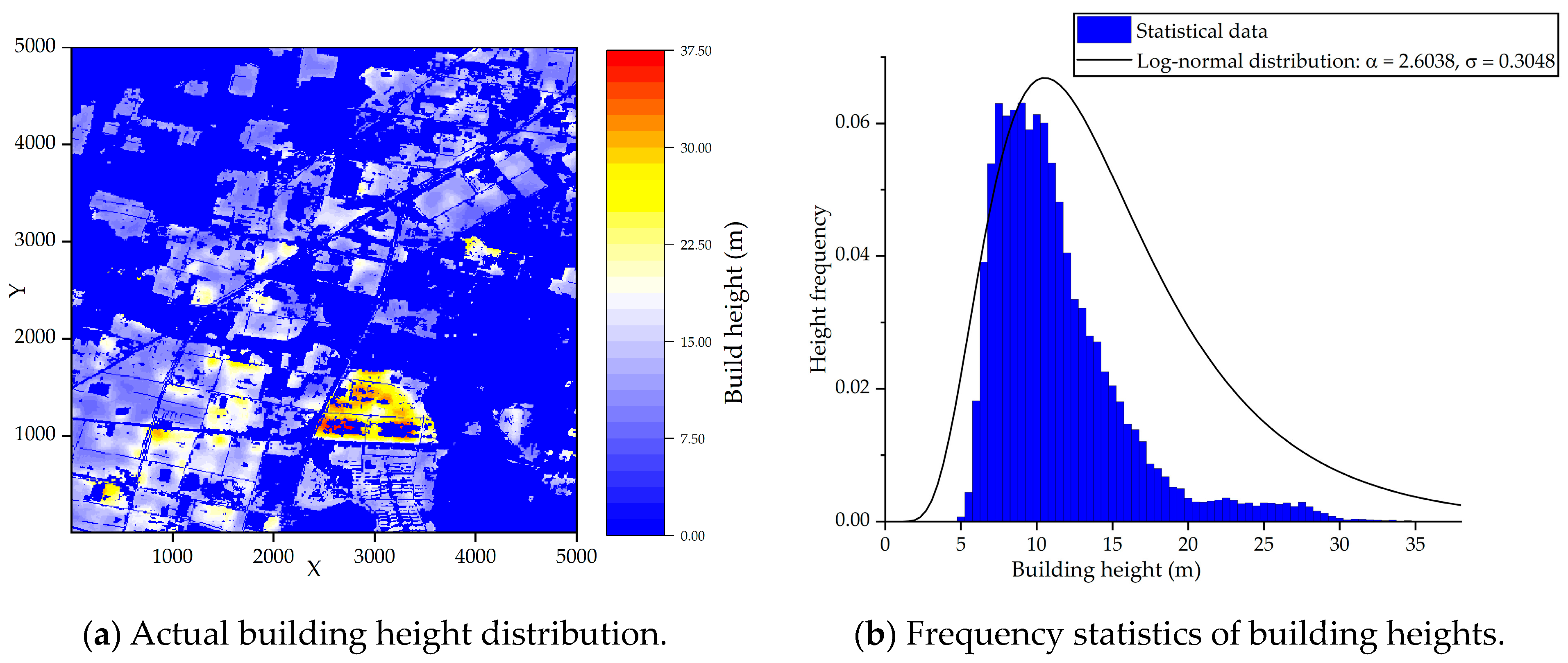
The accurate densities and heights of all the obstacles on the ground are fundamental when a ground obstacle layer is constructed. In this paper, the Chinese building height at 10 m resolution (CNBH-10 m) is the data source for the building densities [26], in which the resolution of a building height map is ten meters. However, due to the lack of specific data, the heights of the trees are defined as a normal distribution, and range from 3 m to 8 m to simulate the actual conditions in the urban environments. Meanwhile, this normal distribution is assumed to have a mean value (μ_tree) of 5.5 and a standard deviation (σ_tree) of 1.25. In this way, based on this assumption, as shown in Equation (8), the tree heights are randomly generated from the normal distribution N(μ_tree, σ_tree) to obtain h_random. Then, the tree heights h_tree are constrained within the range of 3 to 8 m.

$$\begin{array}{l}{h}_{random}\sim N({\mu }_{tree},{\sigma }_{tree}^2)\\ h_{tree}=\max \left\{3,\min (8,h_{random})\right\}\end{array}$$

(8)

4. Risk Assessment and Distribution Estimation

When a UAV failure event happens in the air, the UAV will crash onto the ground, which would further lead to peoples’ injuries or deaths on the ground. Three sequential factors contribute to this complete process, which are UAV malfunctions leading to a crash, descending UAVs colliding with ground obstacles, and the ground casualties caused among pedestrians or property damage to ground buildings [11]. The ground risk caused by crashed UAVs, which is denoted as C_risk, can be finally defined using Equation (9).

$$C_{risk}=P_{crash}\cdot P_{impact}\cdot R_{fatality}$$

(9)

In Equation (9), P_crash is the failure probability of a UAV in the air. P_impact refers to the probability of a UAV impacting people on the ground. R_fatality indicates the probability of people on the ground sustaining fatal injuries after being impacted by the crashed UAV. The detailed discussion of these three factors is provided in the following sections.

4.1. Fatality Risk Cost Model

Equation (9) gives a general idea to calculate the risk imposed by crashed UAVs on people on the ground. Based on this method, the fatality risk can be divided into the direct risk to pedestrians on the ground, and the risk to vehicles on the ground, which further causes injuries to people. This fatality risk model is given in Equation (10).

$$C_{r\_f}=C_{r\_p}+C_{r\_v}$$

(10)

where C_{r_p} means the risk that is imposed on pedestrians on the ground and C_{r_v} is the risk to vehicles on the road. The calculation of C_{r_p} and C_{r_v} is given in detail in the following sections.

4.1.1. Risk Assessment for Ground Pedestrians

Combined with Equation (9) above, the model to estimate the risk imposed to pedestrians on the ground by UAV crashes is given in Equation (11).

$$C_{r\_p}=P_{crash}\cdot P_{p\_i}\cdot R_{p\_f}$$

(11)

In Equation (11), P_crash is the probability that a UAV loses control in the air and crashes onto the ground. The identification of a UAV’s crash probability is so complicated that the historical data in traditional aviation are not suitable for estimating this probability directly. According to Ref. [27], the failure rate for commercial manned aircrafts is set at 1/10⁵ per flight hour, and similarly the failure rate for the UAVs is set at 1/10⁴ per flight hour, which is also used as a reference in this paper. P_{p_i} denotes the number of pedestrians on the ground who are affected by a crashed UAV in urban areas. In order to obtain a more accurate P_{p_i}, the UAV’s complete descent should be analyzed and simulated. There are four typical types of UAV descents, which are the ballistic descent, uncontrolled glide, parachute descent, and flyaway [9]. In this paper, the ballistic descent is considered. This occurs when a UAV loses most of its lift entering a (near) ballistic trajectory, which is entirely governed by its aerodynamics. In this way, P_{p_i} can then be obtained using Equation (12), which is a linear function related to the number of pedestrians on the ground.

$$P_{p\_i}=a\cdot N_p$$

(12)

where a is the slope of the linear function, which can be adjusted based on the characteristics of the ground where the UAV crashes. N_p is the actual number of the pedestrians on the urban ground, which can be obtained using Equation (13). ρ_P is the population density in a ground grid, which is given in Equation (7). S_{u_hit} is the area of ground impact when the UAV crashes to the ground.

$$N_p=S_{u\_hit}\cdot {\rho }_p$$

(13)

Equation (14) shows how S_{u_hit} is calculated. In Equation (14), L_u is the maximum value of the UAV’s dimension. H_p is the average height of the pedestrians on the ground, which is set as 1.75 m in the model. Similarly, R_p is the average radius of the ground pedestrians, which is set to 0.25 m. γ is the angle of descent when the UAVs are falling in the air with the absence of power.

$$S_{u\_hit}=\pi {(L_u+{\displaystyle \frac{H_p}{\tan \gamma }}+2R_p)}^2$$

(14)

Obtaining the parameter γ is given in Equation (15). In this equation, v_u is the UAV’s velocity when descending. m_u is the mass of the UAV. ρ_A is the air density at sea level, whose value is 1.225 kg/m³. C_D is the drag coefficient and A_u means the windward area of the UAV. g is the gravitational acceleration, which is normally taken as 9.8 m/s².

$$\gamma ={\tan }^{-1}{\displaystyle \frac{H_p}{v_u\sqrt{\frac{2m_u}{{\rho }_A{C}_D{A}_{u}g}}{\cosh }^{-1}{e}^{\frac{{\rho }_A{C}_D{A}_u{H}_p}{2m_u}}}}$$

(15)

Figure 6 illustrates the ground areas that could be affected by a UAV’s crash, whose center is the UAV’s failure point projected on the ground.

The fatality rate of people on the ground who are impacted by the crashed UAVs is associated with two main factors, which are the kinetic energy of the UAVs impacting the ground and the sheltering factors that are provided by different ground features. Equation (16) shows the derivation of the fatality rate, which is denoted as R_{p_f}. In this equation, E_k is the mentioned kinetic energy of the UAVs when they impact the ground and S_f is the corresponding sheltering factors that could be provided by different ground features. The value of S_f can be found in Table 2.

$$R_{p\_f}={\displaystyle \frac{1}{1+\sqrt{\frac{\alpha }{\beta }}{\left(\frac{\beta }{E_k}\right)}^{\frac{1}{4S_f}}}}$$

(16)

In Equation (16), α represents the impact energy that may cause a 50% fatality rate when the sheltering factor S_f = 0.5. β indicates a threshold of the impact energy required to cause a fatality when S_f is close to 0 [28]. In this paper, the parameters α and β are set as α = 10⁶ J and β = 100 J, respectively. The impact kinetic energy E_k can be obtained using Equation (17).

$$E_k={\displaystyle \frac{m_u{v}_{hit}^2}{2}}$$

(17)

where v_hit is the velocity of a UAV at the moment that it hits the ground. The calculation for this parameter v_hit is given in detail in the following by analyzing the UAV’s descent process. During a UAV’s descent, its vertical drag resistance F_d is related to the UAV’s mass, size, and air density, which is denoted with Equation (18).

$$F_d={\displaystyle \frac{C_D{A}_u{\rho }_A{v}_{TAS}^2}{2}}$$

(18)

In Equation (18), C_D is the drag coefficient, A_u is the frontal area of a falling UAV, ρ_A is the air density, which is a constant with a value of 1.225 kg/m³, and v_TAS is the true airspeed of a falling UAV (Equation (13)). In this way, the UAV’s acceleration can be represented by Equation (19).

$$a={\displaystyle \frac{F_g-F_d}{m_u}}=g-{\displaystyle \frac{C_D{A}_u{\rho }_A{v}_{TAS}^2}{2m_u}}$$

(19)

In this equation, F_g is the force of gravity, which can be expressed as F_g = m_u⋅g. Thus, the velocity v_hit of a UAV at the moment t when it hits the ground can be obtained with Equation (20) below.

$$v_{hit}={\displaystyle \underset{0}{\overset{t}{\int }}\left(g-\frac{C_D{A}_u{\rho }_A{v}_{TAS}^2}{2m_u}\right)} dt=\sqrt{{\displaystyle \frac{2m_{u}g}{C_D{A}_u{\rho }_A}}\left(1-e^{-{\displaystyle \frac{h{C}_D{A}_u{\rho }_A}{m_u}}}\right)}$$

(20)

It is obvious that h represents the height of the UAV above the ground when it loses control.

4.1.2. Risk Assessment for Ground Vehicles

The risk imposed on the ground vehicles by a UAV’s crash is highly related not only to the kinetic energy of a UAV when it hits the ground, but also the speed and density of the ground vehicles, as well as the probability that a UAV fails in the air [15]. Equation (21) can be used to estimate the risk imposed on the ground vehicles.

$$C_{r\_v}=P_{crash}\cdot P_{v\_i}\cdot R_{v\_f}$$

(21)

where C_{r_v} is the risk to the ground vehicles that is caused by the UAV’s crash. P_crash is the probability that a UAV loses control in the air and crashes onto the ground. P_{v_i} is the number of vehicles that are hit by the crashed UAV. R_{v_f} is the average fatality rate of persons in vehicles that are killed in the accidents.

As shown in Equation (22), the calculation method for P_{v_i} is similar to that for P_{p_i}. S_{u_hit} is the size of the UAV’s crash impact area; ρ_v is the vehicle density.

$$P_{v\_i}=S_{u\_hit}\cdot {\rho }_v$$

(22)

Due to the unavailability of actual vehicle density data, we approximate the vehicle density in the study area using a normal distribution, as shown in Equation (23). Vehicle densities are randomly selected within the range of 0 to 2μ_v. According to the Jinan Municipal Government, by the end of 2023, the total highway mileage in the city was 18,356.5 km, and there were 389.8 million civilian motor vehicles. Assuming an average road width of 25 m, the average vehicle density (μ_v) is approximately 8.49 × 10³ (vehicles/km²). Considering the variability in urban traffic density, the standard deviation (σ_v) is set to 2 × 10³ (vehicles/km²).

$$\begin{array}{l}{\rho }_{v\_random}\sim N({\mu }_v,{\sigma }_v^2)\\ {\rho }_v=\max \left\{0,\min (2{\mu }_v,{\rho }_{v\_random})\right\}\end{array}$$

(23)

In Equation (21), R_{v_f} represents the fatality rate when a UAV crashes into a vehicle, and it can be defined by Equation (24).

$$R_{v\_f}={\displaystyle \frac{1}{1+\sqrt{\frac{\alpha }{\beta }}{\left(\frac{\beta }{E_{v\_k}}\right)}^{\frac{1}{4S_f}}}}$$

(24)

However, in order to calculate the kinetic energy E_{v_k} of the UAV impacting ground vehicles, a relative velocity of the crashed UAV and vehicle is considered, which is denoted in Equation (25). m_u is the mass of a UAV, v_u is the velocity of the UAV at the moment of impact with the vehicle, and v_car is assumed to be the road speed limit.

$$E_{v\_k}={\displaystyle \frac{m_u(v_u^2+v_{car}^2)}{2}}$$

(25)

4.2. Property Damage Risk Cost Model

Dense high-rise buildings in urban environments present another challenge for UAV operations, as potential collisions with buildings during a UAV’s flight pose the risk of property damage. The lower the flight altitude of a UAV, the higher the density of buildings encountered, which increases the operational risk and reduces the efficiency [13]. Conversely, in areas with fewer buildings, the safety of UAV operations is enhanced. The distribution of building heights in urban areas follows a log-normal distribution, and the values of different buildings vary. Thus, the property damage risk cost C_{r_b} can be established with Equation (26).

$$C_{r\_b}=\{\begin{array}{l}{\alpha }_b\psi (e^{\mu })0<h\le e^{\mu }\\ {\alpha }_b\psi (h)h>e^{\mu }\end{array}$$

(26)

In Equation (26), ψ(h) can be defined further using Equation (27). h is the building height. μ and σ are the mean and standard deviation of the logarithmic variable. α_b (α_b ∈ (0, 1]) is defined as a coefficient for different building categories, and is used to adjust the effects on the risk based on the types of buildings.

$$\psi (h;\mu ,\sigma )={\displaystyle \frac{1}{h\sigma \sqrt{2\pi }}}{e}^{-{\displaystyle \frac{{\left(\ln h-\mu \right)}^2}{2{\sigma }^2}}}$$

(27)

Table 3. Building types and corresponding α_b.

Building Types	αb
Blue-Roofed Shed, Red-Roofed Shed	0.25
Tile Low Building (brown, gray, red)	0.50
Industrial Area (silver-grey, white-blue)	0.80
High-Rise Structure	1

shows possible building types in urban areas and their corresponding values of coefficient α_b. The Blue-Roofed and Red-Roofed Sheds share the same α_b with the value of 0.25. The Tile Low Building’s α_b is 0.50. The Industrial Area and High-Rise Structure have values of α_b of 0.80 and 1, respectively.

4.3. Integrated Risk Cost Model

All the risks introduced by UAV operations in urban areas consist of the fatality risk cost and property damage risk cost. Generally, the weight of the fatality risk is considered to be the most critical because of the most significant severity. Although reducing the weight of property damage risk may increase the UAV operation cost in some situations, it would prevent or mitigate the casualties and lessen the negative impact on society. Furthermore, given the differences in the order of magnitude for different types of ground risk, a normalized factor ω_i is designed with a normalization range of (0, 1]. Therefore, the integrated risk cost model is developed as a linear model, which is given in Equation (28).

$$C_u={\displaystyle \sum _{i=1}^2{\alpha }_i\cdot {\omega }_i\cdot C_i}$$

(28)

In Equation (28), C_u is the integrated risk cost. α_i (i = 1, 2) indicates a weight factor with α_i ∈ (0, 1] and α₁ + α₂ = 1. ω_i is a normalized factor and ω_i = 1/C_{i_max}. So, in this situation C_{i_max} is the maximum possible value for each type of ground risk. C_i is the value of ground risk, and it should be noted that {C_i: C₁ = C_{r_f}, C₂ = C_{r_b}}.

4.4. Estimation of Risk Distributions

In this paper, a ground risk map is constructed as a three-dimensional cuboid with each unit having resolution of 1 m × 1 m × 5 m. Within each cuboid, the risk is represented as C_{u,1_1_5}(x, y, z), where (x, y, z) is a 3D coordinate. Operating in a high-resolution map enables UAVs to avoid the high-risk areas, significantly enhancing flight safety. However, a high-resolution map also presents certain challenges. For example, a high-resolution map requires a much larger storage space and greater processing power. Additionally, in some low-risk areas, the UAVs can traverse directly without complex data processing, yet the high-resolution maps significantly increase the computational burden. To address this problem, a method for converting the resolution of a risk map is proposed, which is shown in Equation (29).

$$C_{u,n\_n\_m}(i,j,k)={\displaystyle \frac{1}{n^{2}m}}{\displaystyle \sum _{a=1}^n{\displaystyle \sum _{b=1}^n{\displaystyle \sum _{c=1}^m{C}_{u,1\_1\_5}(ni+a,nj+b,mk+c)}}}$$

(29)

The risk of a specified urban area can be represented either by the average value of the risk or by the maximum value of the risk. In this study, to obtain a risk map in another resolution, the averaging method is used to calculate the risk value in the converted map. As given in Equation (29), C_{u,n_n_m} is the value of the risk within a new cuboid with a size of n × n × m. i, j, and k are the indices of a new cuboid in the x, y, and z directions, respectively. a, b, c are used to iterate over the positions in the original map relative to the corresponding cuboids in the new map.

5. Simulations and Verifications

In this section, a case study is presented to illustrate the proposed methodology. First, each risk layer is generated based on the classification of a satellite image from the actual urban environment. Subsequently, a risk assessment model is implemented to generate a three-dimensional risk map. The model and algorithm were coded in MATLAB and ran on a server with a 5.4 GHz CPU and 32.0 GB of RAM.

5.1. Scenario Description

An actual urban area of Changqing District in Jinan City is selected for UAV operations. The satellite image of this area is given in Figure 7, whose size is 5 km × 5 km. As shown in Figure 7, the typical urban elements are incorporated in this area representing the characteristics of a modern city. The ground features in the satellite image given in Figure 7 can be classified into 15 types based on the classifications given in Table 1. From this figure, it can be seen that a lot of areas in the bottom left are predominantly residential quarters with a uniform housing structure, which correspondingly indicates a densely populated area.

Risk assessment was conducted using a model M210RTK UAV, which is manufactured by DJI. The DJI M210RTK is a type of rotor-wing vertical take-off and landing (VTOL) aircraft, which is commonly utilized in fields such as public safety, civil security, environmental management, and disaster monitoring and control. The parameters of the UAV DJI M210RTK are given in

Table 4. Parameters of UAV M210RTK.

Parameter	Value
Mass	4.27 kg
Length	0.887 m
Width	0.880 m
Frontal Area	0.234 m2
Pcrash	3.42 × 10−4

, including the mass, length, and width, which are 4.27 kg, 0.887 m, and 0.880 m. The frontal area of this UAV is 0.234 m². The probability of the UAV failure in the air is also given in Table 4, which is 3.42 × 10⁻⁴.

Table 5. Parameters for risk assessment.

Parameter	Value
g	9.8 m/s
ρA	1.225 kg/m3
CD	0.3
vcar	16 m/s
α	106 J
β	100 J

provides the needed parameters when assessing and estimating the risk caused by the UAV operations in urban areas. The density of the air is 1.225 kg/m³ and the drag coefficient is set as 0.3. The values of parameters α and β are set as 10⁶ J and 100 J, respectively. The velocity of all ground vehicles is set to the same value of 16 m/s.

In order to construct multiple map layers, two data sources are used. The first is the population distribution data, which delineate the number of people per grid cell with a resolution of 100 m × 100 m. The second is the building height data, which provide the information about the heights of ground buildings with a resolution of 10 m × 10 m, aiding in the analysis of the three-dimensional structure of urban areas.

5.2. Classification Results of the Satellite Image

The ground features in a satellite image are classified based on their RGB values. The selected satellite image consists of 5000 × 5000 pixels in total, and the resolution of each pixel is 1 m × 1 m. Fifteen ground features are defined in Table 1. At the beginning, the initial clustering centers are selected randomly to ensure the randomness of the starting points of the K-Means clustering algorithm. The clustering process continues iteratively until the clustering centers no longer change, at which point the final clustering results are returned to further ensure the stability and accuracy of the outcomes. After the K-Means clustering operation is completed, a similarity matching process is then performed according to the obtained results. Figure 8 shows the classification results of a selected satellite image, which gives the spatial distribution of various types of ground features.

As shown in Figure 8, a specific color identifies each ground feature. Among these, Woody Plant has the widest distribution, covering 14.7% of the study area, mainly concentrated around the coordinates (1000, 3700) and (4000, 2500). Carriageway ranks second with a proportion of 12.9%, with several main roads clearly visible traversing the study area. Lawn and Blue Construction Site are the third and fourth most common ground features, accounting for 11.5% and 10.6% of the area, respectively. Red-Roofed Shed has the least distribution, occupying only 1% of the area. The proportions of all ground features are shown in Figure 9, starting from 1.6% for Loess and displayed in a clockwise order, showing the proportion of each ground feature.

5.3. Generation of a Population Density Layer

Figure 10a shows the original population density, whose data are from WorldPop. The size of each grid cell in Figure 10a is 100 m × 100 m. It can be seen that the population is primarily concentrated in the bottom left, which is proven to be a densely populated residential district. Notably, the grid cell located near the coordinates (800, 1300) has the highest population density, with a maximum value of 175.238. This pattern of ground population distribution aligns with the typical layout of the urban residential areas, which is shown in Figure 8. The high-density housing areas usually correspond with the concentration of the ground population in city centers. The population in this selected region is about 77,904. The Seventh National Census reported approximately 68,619 people in the same area. The difference between the two estimates is 9285 people. Using Equation (3), the correction coefficient C_c is calculated as 0.8808.

Based on the assumptions that each type of ground feature is associated with a specific population density, we derived the population densities for each ground feature using a regression model, as shown in

Table 6. Population density of ground features.

Ground Feature	Population Density (10−3 People/m2)
High-Rise Structure	6.7441
Red Tile Low Building	3.7066
Brown Tile Low Building	3.0889
Gray Tile Low Building	2.5384
Blue-Roofed Shed	3.6033
Red-Roofed Shed	2.4022
Silver-Grey Industry	2.2052
White-Blue Industry	17.6416
Blue Construction Site	2.8910
Concrete Floor	3.5808
Lawn	1.5021
Woody Plant	1.5022
Carriageway	4.2970
Lake	0
Loess	2.9962

. The highest population density is found in the industrial areas, with a value of 1.7642 × 10⁻² people/m². It should be noted that since in Lake areas there is no population, the population density is set to zero correspondingly. The population density of the High-Rise Structures is 6.7441 × 10⁻³ people/m². The Carriageway’s population density is 4.2970 × 10⁻³ people/m². The Red Tile Low Building, Blue-Roofed Shed, and Concrete Floor share a similar population density, with the values of 3.7066 × 10⁻³ people/m², 3.6033 × 10⁻³ people/m², and 3.5808 × 10⁻³ people/m², which are a little higher than that of Brown Tile Low Building, with the value 3.0889 × 10⁻³ people/m². The population densities of the Gray Tile Low Building, Red-Roofed Shed, Silver-Grey Industry, Blue Construction Site and Loess are between 2 × 10⁻³ people/m² and 3 × 10⁻³ people/m². The Lawn and Woody Plant’s population densities are more or less the same, with values of 1.5021 × 10⁻³ people/m² and 1.5022 × 10⁻³ people/m², respectively.

To create a more accurate population density layer, the data from WorldPop and the population density corresponding to ground features are combined using Equation (7), with weight coefficients set to 0.3 and 0.7, respectively. The resulting population density layer, as shown in Figure 10b, has a resolution of 1 m × 1 m. This layer clearly illustrates the population distribution across the entire selected urban area. For instance, the Lake areas centered around coordinates (500, 2700) and (4000, 1800) have a population density of 0, depicted as dark purple in Figure 10b. The highest population density is located at (701, 1278), with a value of 0.0176 people/m², corresponding to the Gray Tile Low Building feature. Most of the population is still concentrated in the bottom left corner of the study area, which is primarily residential. Another high-density area is around (2000, 4000), where the ground feature is Industry, which is logical due to the presence of many workers.

5.4. Generation of a Sheltering Factor Layer

The sheltering factors of different ground features are defined within the range of 0 and 1, which are used as the needed parameters in Equation (16). A sheltering factor quantifies the probability of fatal injuries caused to the exposed personnel in a UAV’s crash event. Each type of ground feature is assigned a corresponding sheltering factor, as detailed in Table 2. Based on the classification results of the satellite image, a sheltering factor layer is constructed, which is shown in Figure 11.

Figure 11 illustrates the spatial distribution of the sheltering effects provided by different ground features across different ground regions. The resolution of this generated sheltering factor layer is 1 m × 1 m, which allows for a more accurate representation of the sheltering effects in different ground areas. In Figure 11, the red areas would provide more sheltering effects that offer better protection to people on the ground. The blue regions represent no sheltering effects, introducing more ground risk. The most notable observation in the figure is that the area with the poorest sheltering effect is the Lake, with a sheltering factor of 0 and a population density of 0. The regions with a sheltering factor ranging from 0.3 to 0.5 are primarily shown in light blue; these areas mainly consist of Woody Plants, which are the most widely distributed ground features in the study area. The areas with higher sheltering factors are primarily residential districts in the bottom left corner, as buildings provide substantial sheltering effects. The most prominent red areas represent the industrial zones, mainly centered around the coordinates (2000, 4000). These industrial zones have high sheltering factors due to the dense concentration of industrial features, and they cover a significant proportion of the area, with White-Blue and Silver-Grey Industrial Areas accounting for a total of 10.5%. Consequently, these areas are quite prominent. The High-Rise Structures have a sheltering factor of 1 but only cover 4.4% of the area, making them less noticeable in the figure. These High-Rise Structures are primarily located around the coordinates (3000, 1000).

5.5. Generation of a a Ground Obstacle Layer

Figure 12 shows the distribution of ground building heights in the selected region, as described in Figure 7. It can be found that, in Figure 12a, the highest ground building reaches 37.47 m and the average ground building height is 14.16 m. The ground building height is subject to a lognormal distribution, as demonstrated in Figure 12b, with mean μ = 2.6038 and standard deviation σ = 0.3048. For the ground features classified as Woody Plant, we also consider them as obstacles, and their heights are randomly determined using a normal distribution model. The average height of the ground trees is set at 5.5 m, and heights range from 3 m to 8 m.

As shown in Figure 12a, the red areas indicate regions with tall buildings, with the tallest building reaching 37.47 m, located at the coordinates (2758, 1105). The buildings around this coordinate are the tallest in the study area. Correspondingly, the population density in this area is also relatively high in the population density layer. The building heights in the bottom left corner of the study area are also significant, ranging from 10 m to 30 m, and the population density is similarly high, indicating a higher risk for UAV operations. The building heights in the upper right corner of the study area are also notable, where many industrial areas are located, with heights around 15 m. The blue areas represent regions with no height, such as the Lake centered at coordinates (4000, 1800); this area also has no population density, resulting in a lower risk for UAV operations.

5.6. Generation of a Risk Map Based on Multiple Layers

In the simulation, the weight coefficients of the ground fatality risk and the property damage risk are set as 0.65 and 0.35, respectively, which are needed in Equation (28). To comprehensively assess the risk at different flight heights, 20 flight levels ranging from 5 m to 100 m are established with an increment of 5 m per level. Six layers of the generated risk map at different flying heights with a resolution of 1 m × 1 m × 5 m are given in Figure 13, which are Layer 1, Layer 5, Layer 9, Layer 10, Layer 15, and Layer 20.

In Figure 13a, with the height of 5 m, the risk of Layer 1 is relatively high, primarily due to the dense distribution of the buildings in an actual urban environment, which leads to a significant increase in the property damage loss, and thereby the total risk rises. When the flight altitude increases as shown in Figure 13b, the property damage risk significantly decreases. The total risk of Layer 5 reduces by 29.68% compared with that of Layer 1. In Layer 9, which is shown in Figure 13c, with the flight altitude of 45 m, there are no buildings at this level and in this way only the risk of fatalities exists. Combining Equation (14) with Equation (15), the higher the operation altitude of the UAVs, the greater the speed and impact area when it uncontrollably falls to the ground. Correspondingly, more risk results. The total fatality risk of Layer 15 is increased by 23.25% compared to that of Layer 10. Layer 20 is 11.61% higher than Layer 15. Overall, the risk is relatively low from Layer 5 to Layer 10. Thus, the UAV operations between these layers pose little risk, meaning these are safer altitudes for UAV flights. Overall, in areas with high population density and a dense building distribution, the risk values are higher. For example, the residential district in the bottom left corner has a high population density, resulting in higher risk values, shown in red in the figure, with risk values around 0.7. The Lake area has very low risk, close to 0, and is prominently displayed in blue in the figure. The Carriageway also shows significant risk due to the presence of ground vehicles, with risk values around 0.5.

Figure 13 shows the risk distributions accurately based on the multi-layer method with a resolution of 1 m × 1 m × 5 m. To better explore the accuracy of the risk distributions under different resolution settings, Figure 14 shows a risk map with a resolution of 50 m × 50 m × 10 m.

It is important to note that since the risk in 14 is represented by the average risk across the area, the high-risk areas may be underestimated, resulting in an overall lower risk. The highest risk value is 0.5344, mainly concentrated in the bottom left corner. However, the risk map presented in 14 exhibits similar characteristics to the previous one, with relatively lower risks in the middle layers. This risk map still holds significant value, as its risk distribution is also representative.

In the first layer, as shown in 14a, buildings around 10 m high are relatively numerous, making the building risk particularly prominent, with a risk value of approximately 0.4, depicted in cyan. At the third layer, with a height of 30 m, the overall risk is below 0.3. Buildings of this height are less frequent, resulting in lower risk. As the height increases, by the fifth layer, there is no property damage risk, and fatality risk becomes dominant. Compared to other layers, the risk in the middle layers (third to sixth layers) is relatively low. In the seventh layer, as shown in 14d, the risk in densely populated areas is more pronounced, such as in the bottom left corner of the study area. In the subsequent layers, the risk values gradually increase, and similar to previous analyses, the rate of risk increase slows down. The total risk of the eighth layer is 15.59% higher than that of the sixth layer, and the total risk of the tenth layer is 9.14% higher than that of the eighth layer.

6. Conclusions

In this paper, a mechanism of risk assessment and its distribution estimation for UAV operations by extracting the ground features from an actual satellite image is proposed. An accurate risk map can be generated using a multi-layer method in urban areas. First, an actual satellite image of a selected city area is classified with a K-Means clustering method and fifteen ground features are extracted. Three more map layers are generated, which are a population density layer, a sheltering factor layer, and a ground obstacle layer. Based on the three established layers, the risk caused by UAV operations is evaluated and calculated by considering the fatality risk and property damage risk. Using a UAV M210RTK, which is manufactured by DJI, as a case study, a comprehensive risk map of specified city areas is generated by overlaying the three obtained map layers. According to the simulations and verifications, there is little risk when the UAV operates between Layer 5 and Layer 10, which proves that these altitudes are relatively safe and suitable for UAV operations. Conversely, more risk is imposed at other altitudes. Additionally, a resolution conversion method is employed to generate risk maps of different resolutions to satisfy different flight requirements.