Quality and Efficiency of Coupled Iterative Coverage Path Planning for the Inspection of Large Complex 3D Structures

Abstract

To enable unmanned aerial vehicles to generate coverage paths that balance inspection quality and efficiency when performing three-dimensional inspection tasks, we propose a quality and efficiency coupled iterative coverage path planning (QECI-CPP) method. First, starting from a cleaned and refined mesh model, this was segmented into narrow and normal spaces, each with distinct constraint settings. During the initialization phase of viewpoint generation, factors such as image resolution and orthogonality degree were considered to enhance the inspection quality along the path. Then, the optimization objective was designed to simultaneously consider inspection quality and efficiency, with the relative importance of these factors adjustable according to specific task requirements. Through iterative adjustments and optimizations, the coverage path was continuously refined. In numerical simulations, the proposed method was compared with three other classic methods, evaluated across five aspects: image resolution, orthogonality degree, path distance, computation time, and total path cost. The comparative simulation results show that the QECI-CPP achieves maximum image resolution and orthogonality degree while maintaining inspection efficiency within a moderate computation time, demonstrating the effectiveness of the proposed method. Additionally, the flexibility of the planned path is validated by adjusting the weight coefficient in the optimized objective function.

1. Introduction

When performing visual inspections of large three-dimensional (3D) structures, it is crucial to capture complete and high-quality target information with high efficiency. However, manual inspection suffers from low operational efficiency, lacks guaranteed complete coverage, is highly subjective, and involves high risk factors [1,2]. To effectively mitigate these issues, automatic inspection using unmanned aerial vehicles (UAVs) equipped with cameras and other sensors has become an important research topic. Coverage path planning (CPP) is a key technology for automatic inspection. The objective of CPP is to plan an optimal path that avoids collisions and obstacles, ensuring that UAVs can utilize their sensors to cover the region of interest (ROI) effectively. Over the past decade, CPP has been successfully applied in fields such as visual inspection of complex structures [3], regional exploration [4,5,6], agricultural operations [7,8], and aircraft skin damage detection [9,10].

To simplify the CPP problem, most studies design two steps [11,12,13]: (1) determine the viewpoint set that can cover the ROI and (2) solve the transversal order of viewpoints and connect them to obtain the final path. In fact, there are many sets of viewpoints that can cover the ROI, and each viewpoint set corresponds to a different path cost, such as path length and energy consumption. Because the focus in the viewpoint generation step is primarily on achieving full coverage, it cannot be guaranteed that the viewpoint set will obtain a good path cost during the path planning step. Therefore, some studies [14,15,16,17,18,19,20] attempt to couple these two steps together through iterations, adjusting the set of viewpoints continuously to obtain a path with a lower cost. In [14,15], based on an initial viewpoint set and coverage path, a new candidate for each viewpoint $q_j$ is iteratively selected to achieve a shorter path length and observe all primitives uniquely observed by $q_j$, facilitated by an enhancement of the rapidly exploring random tree (RRT) algorithm [16]. Unlike selecting a new candidate through random sampling, the methods proposed in [17,18] determine an improved set of viewpoints that achieve complete coverage while reducing path length by solving a quadratic problem. Reference [19] enhances the inspection path using remeshing techniques via an iterative strategy, achieving uniform coverage of the 3D structure with high computational efficiency. Reference [20] combines path optimization algorithms with the particle swarm optimization (PSO) framework, using random sampling for path initialization. In most of these CPP methods, the path is typically initialized using random sampling methods, without considering the regularity of viewpoint generation and image quality. Consequently, the initially chosen path shape may be overly cluttered, and the inspection quality cannot be ensured. This will make subsequent optimization difficult.

For certain structure inspection tasks, such as detecting aircraft skin damage, high-quality images are crucial for achieving precise identification of damages of various sizes. However, most existing CPP methods prioritize minimizing path distance and ensuring complete coverage, often neglecting image quality as a specific objective in path planning. A model-based CPP method was proposed in [21] to generate paths that maximize coverage ratio while minimizing path distance, utilizing a heuristic reward function developed based on the structural mesh model and UAV-mounted sensors. Reference [22] proposed a CPP method that utilizes a multi-resolution hierarchical framework, addressing the problem at two different levels and emphasizing the improvement of path generation efficiency. To enhance the coverage path accuracy and coverage ratio of the primal sampling method, an adaptive search space coverage path planner (ASSCPP) was proposed in [23], which combines the model of the structure to be inspected with the noise model of the onboard sensors to generate paths. The algorithm generates a set of viewpoints through adaptive sampling, directing the search towards areas with low coverage accuracy and ratio. Reference [24] proposed a two-stage automatic aircraft scanning method using UAVs equipped with RGB-D cameras. In the first stage, the UAV–camera system follows a predefined path at a distance from the aircraft surface to generate a coarse model of the aircraft. Subsequently, an optimal scanning path, defined as the shortest flying distance for full coverage, is computed using a Monte Carlo tree search algorithm. Reference [25] designed a non-random targeted viewpoint sampling strategy to reduce the number of viewpoints, which can significantly shorten the cycle time for the inspection task. References [26,27] focused on additional indices such as turning angle, path distance, battery capacity, etc., without explicitly considering the quality of captured images. Unlike previous studies that separately address CPP and trajectory planning, reference [3] innovatively tackles both issues simultaneously. It proposed a multi-UAV collaborative coverage trajectory planning method based on heat equation driven area coverage and demonstrated its application on various complex 3D structures, achieving significant results. Most CPP methods do not integrate image quality into path optimization, often failing to align inspection quality with efficiency. Consequently, the planned paths may lack flexibility for user-defined adjustments. In structural surface inspection, focusing solely on inspection quality can lead to unnecessarily long paths and extended execution times. Conversely, prioritizing inspection efficiency alone may result in capturing images that inadequately represent critical structural defect features for accurate analysis. Therefore, achieving both high inspection quality and efficiency is crucial.

In practice, large 3D complex structures often feature narrow spaces, such as the area beneath an aircraft’s belly, where the movement of a robot is restricted. Current methods typically employ primal sampling for such spaces [14,15]. However, when the detection sensors carried by the robot have multiple degrees of freedom, sampling numerous viewpoints in discrete spaces escalates computational complexity significantly. Thus, a common dilemma arises between achieving high coverage ratio and managing computational demands when using primal sampling-based CPP methods. Inspection in narrow spaces necessitates the consideration of factors such as the UAV’s minimum flight altitude, shooting distance, size of the primitive to be inspected, and quality of the captured images. Inadequate attention to these factors may result in the exclusion of inspected areas, leading to substantial reductions in both coverage ratio and inspection quality [28].

To address the aforementioned challenges, we propose a quality and efficiency coupled iterative coverage path planning (QECI-CPP) method. This approach considers narrow spaces and emphasizes high-quality initialization to generate a coverage path that balances inspection quality and efficiency. The method employs iterative optimization based on a novel objective that integrates both quality and efficiency considerations.

The contributions of this work are as follows:

• A quality-guided and non-random dual sampling inspection strategy is employed to obtain the initial viewpoint set, enhancing conditions for subsequent iterative path optimization. Additionally, to accommodate narrow spaces using dual sampling methods, specific adjustments are made to the sizes of surface triangles on the structure surfaces near these spaces, along with the constraints on the feasible viewpoint space associated with each surface triangle.
• A dual-coupling strategy is proposed for CPP. Initially, viewpoint generation is integrated with path planning, continuously optimizing the viewpoint set and coverage path to lower path costs through iterations. Additionally, the objective function for iterative optimization is designed to integrate metrics including image resolution, orthogonality degree, and path length, thereby coupling coverage quality with efficiency. Particularly, the introduced weight coefficient in the objective function can be flexibly adjusted to meet the specific requirements of various inspection tasks concerning coverage quality and efficiency characteristics.

The paper is organized as follows. Section 2 describes the CPP problem. Section 3 introduces the primary strategies of the proposed method. Section 4 presents the evaluation metrics for coverage paths and includes comprehensive simulation comparisons. Section 5 provides the concluding remarks.

2. Problem Description

2.1. Model Description

To perform the QECI-CPP design, the following models are employed.

• Three-dimensional structure model: The 3D structure model to be inspected is represented using surface triangles. Initially, this model can be rough since it will undergo cleaning, refinement, and adjustment of surface triangle size during the preprocessing step of the proposed method.
• UAV model: As an example, we consider a common rotary-wing UAV equipped with a gimbal camera. The gimbal camera is not fixed to the UAV body but can move independently, expanding the accessible space of the viewpoint.
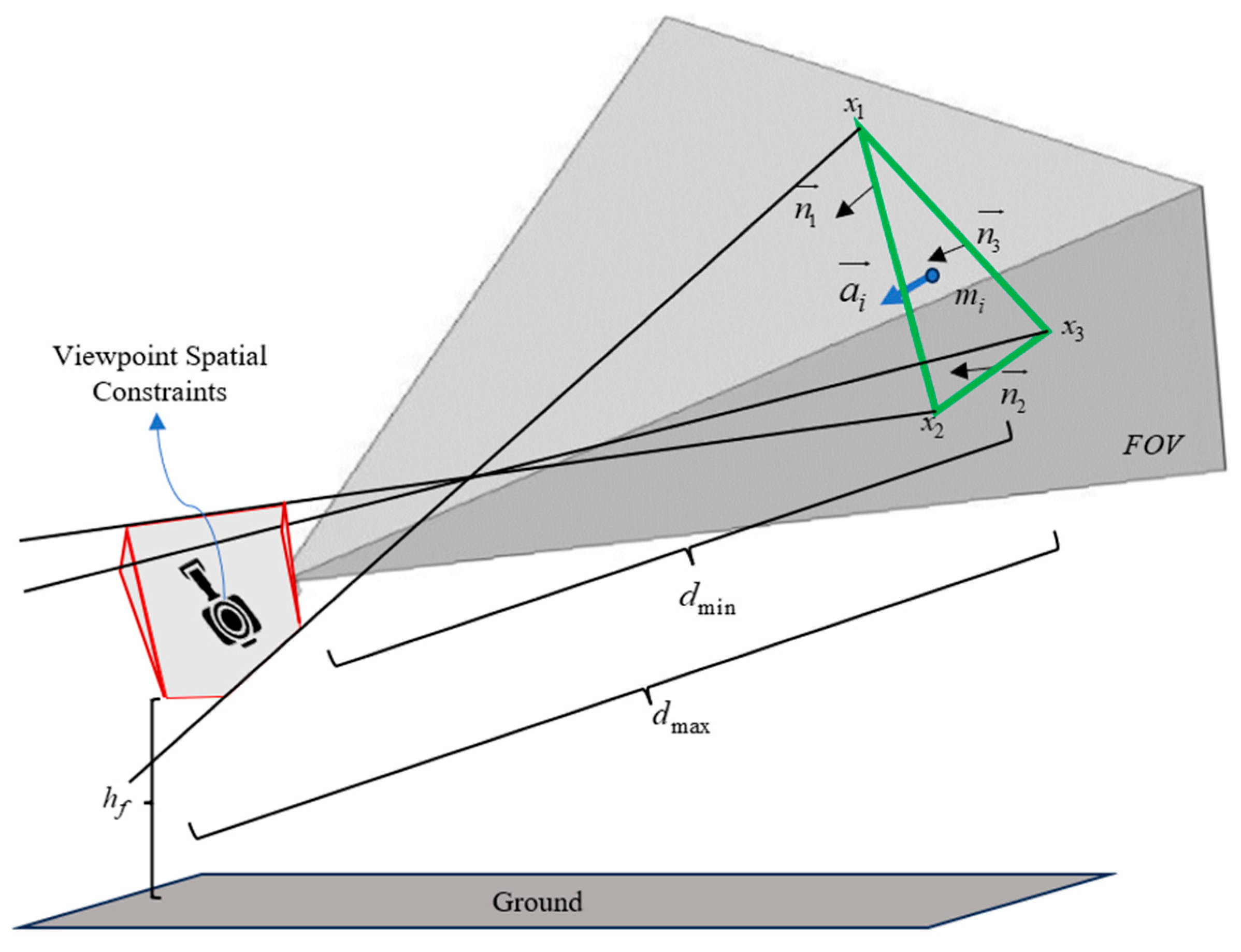
• Pan–tilt (PT) camera model: The PT camera model is defined by its frustum and orientation [29]. The shape of the frustum is determined by the corresponding field of view (FOV) as well as the minimum and maximum detecting ranges. The orientation and shutter of the PT camera are controlled by a gimbal stabilizer. Since most PT cameras do not have restrictions on yaw angles [30], we assume a yaw angle range of $[-\pi ,\pi ]$. As a result, the camera orientation is only restricted by the pitch angle. The PT camera is precalibrated with its radial distortion removed, and its parameters such as FOV and focal distance range are known in advance.

2.2. Definition of Inspection Quality and Inspection Efficiency

• Orthogonality degree and resolution are used to evaluate the quality of captured images. The orthogonality degree measures the deviation of the camera’s shooting direction from the normal vector direction of the surface triangle. Our goal is to align the camera’s shooting direction as closely as possible with the normal vector of the surface triangle to minimize side-angle shots and reduce image distortion. Resolution refers to the clarity of the camera’s captured surface features. For a given surface triangle and specific camera parameters, optimal view-to-surface resolution is achieved by determining the viewpoint where the projected image best fits the surface triangle. Detailed mathematical descriptions of these performance metrics will be provided later.
• Inspection Efficiency: The path distance is closely related to the efficiency of completing the task. Therefore, in this paper, the distance of the coverage path is used to represent inspection efficiency.

2.3. Problem Formulation of CPP

For the given models of structure, UAV, and sensor, the optimization goal of CPP is to plan a high-quality and efficient path under the constraints of full coverage and feasible movement space of the UAV. Additionally, the path’s balance between inspection quality and efficiency can be adjusted based on user-defined priorities.

3. Proposed Methodology

The workflow of our proposed CPP method is illustrated in Figure 1. Firstly, in the preprocessing step (Section 3.1), the mesh model of the 3D structure undergoes refinement and cleaning. To accommodate narrow space environments with restricted movement, sizes of the surface triangles are adjusted according to different spatial constraints. Subsequently, an initial viewpoint for each surface triangle is selected (Section 3.2). The generation of these viewpoints ensures high resolution and orthogonality. Once the initial viewpoints are determined, they are sequentially connected to form the initial path. The primary consideration during viewpoint generation is path quality, while path efficiency becomes paramount during path generation. Finally, to optimize the path further and reduce total cost, an iterative resampling scheme is employed (Section 3.3). Between each resampling iteration, viewpoints are continuously updated according to an objective function that integrates inspection quality and efficiency. Once a satisfactory path is found, the final step is to deploy the computed path as the flight path.

3.1. Model Preprocessing

To plan a high-quality coverage path adaptable to narrow spaces, the preprocessing phase involves cleaning and refining the provided mesh model. Specific constraints must be set for areas where UAV movement is restricted. For instance, consider the inspection of a civil aircraft: above the aircraft, the UAV enjoys greater freedom of movement, allowing it to capture comprehensive surface information from a suitable distance, thus minimizing the number of viewpoints required. Conversely, beneath the aircraft, movement space is limited, potentially hindering the complete coverage of the surface triangle if the surface triangle is too large. Attempting to capture images from a distance may risk collisions with the ground. Therefore, to ensure both a high-quality coverage path and UAV safety, the adjustment of surface triangle sizes should be tailored to suit the characteristics of different spaces. Subsequently, the length of the camera’s view range in various spaces is first calculated. Then, we assess whether the actual size of the surface triangle fits within this FOV. If not, adjustments are made to the surface triangle accordingly.

The actual length of the camera’s view range at a certain distance is calculated as:

$$H_x=h_x\times d/f,H_y=h_y\times d/f$$

(1)

where $f$ represents the focal length of the camera; $d$ represents the distance between the camera and the target surface triangle; $h_x$ and $h_y$, respectively, represent the length and width of the camera’s image sensor size; and $H_x$ and $H_y$, respectively, represent the length and width in the actual FOV. For the space above the aircraft (the height exceeds the threshold $h_l$), let $d_{max}$ and $d_{min}$ be the maximum and minimum shooting distances between the camera and the target surface triangle; and for the space beneath the aircraft (the height is below the threshold $h_l$), let $d_{l\_max}$ and $d_{l\_min}$ be the maximum and minimum shooting distances. Then, the maximum and minimum values of $H_x$ and $H_y$ for various spaces can be calculated based on Equation (1), which are denoted by $H_{x\_max}$, $H_{x\_min}$, $H_{y\_max}$, and $H_{y\_min}$, respectively. Figure 2 is a schematic diagram of the size relationship between the target surface and the image.

For convenience, a simplified rectangle is used to approximate the camera view. Figure 3 illustrates the schematic diagram depicting the size relationship between the camera view and the surface triangle, where $m_i$ represents the centroid of the i-th surface triangle, and $l_{jx}$ and $l_{jy}$ $\left(j=1,\hspace{0.17em}2,\hspace{0.17em}3\right)$ represent the horizontal and vertical distances from each of the three vertices of the surface triangle to $m_i$. During constraint calculations, the centroid of the surface triangle overlaps with the center point of the rectangle, and the constraints are established separately as follows:

$$H_{x\_min}/2\le l_{jx}\le H_{x\_max}/2$$

(2)

$$H_{y\_min}/2\le l_{jy}\le H_{y\_max}/2$$

(3)

Using Rhino 7 and CINEMA 4D R18 modeling software, the area of each original surface triangle is checked. If a surface triangle does not meet the above conditions, its size is constrained to the corresponding maximum or minimum value. For a given camera model, if high-resolution images are required, it is crucial to reduce $d_{max}$ and $d_{min}$. Once the image resolution requirements are established, $d_{max}$ and $d_{min}$, as well as $H_{x\_max}$, $H_{x\_min}$, $H_{y\_max}$, and $H_{y\_min}$, are determined. Then, we use the method outlined above to adjust the size of each surface triangle. If a surface triangle exceeds the maximum coverage of a single image, we subdivide it so that each surface triangle meets the resolution requirements. This process not only yields a high-resolution mesh model but also allows us to plan a coverage path that captures high-resolution images.

3.2. High-Quality Initial Path

Here, we first introduce the viewpoint spatial constraints of the surface triangle, and then discuss the strategies for initializing high-quality viewpoints.

3.2.1. Spatial Constraints Applied to Viewpoints

For each surface triangle in the 3D structure to be inspected, a viewpoint must be found that can capture its image. Therefore, the spatial constraints for the viewpoint need to be defined. Figure 4 illustrates the schematic diagram of spatial constraints applied to a viewpoint. $V_i=[x,y,z]$ is denoted as the position of the viewpoint of the i-th surface triangle ($i=1,2,\cdots ,T_n$, $T_n$ represents the total number of surface triangles), and then the specific constraints for $V_i$ are defined as follows:

$${(V_i-x_j)}^T\cdot \overrightarrow{n_j}\ge 0$$

(4)

$${\overrightarrow{a_i}}^T\cdot (V_i-x_1-d_{min}\times \overrightarrow{a_i})\ge 0$$

(5)

$${\overrightarrow{a_i}}^T\cdot (V_i-x_1-d_{max}\times \overrightarrow{a_i})\le 0$$

(6)

$$V_i[2]\ge h_f$$

(7)

$${\theta }_k(V_i,m_i,x_l,x_r,x_t,x_b)\le {\theta }_k\hspace{0.17em}\left(k=h,v\right)$$

(8)

$${\theta }_g(V_i,m_i)\in [{\theta }_{min},{\theta }_{max}]$$

(9)

where $x_j(j=1,2,3)$ is the coordinate vector of the three vertices of the surface triangle; $\overrightarrow{n_j}$ is the normal vector of the j-th separating hyperplane, which forms an angle ${\theta }_c$ with the surface triangle and intersects the j-th edge of the surface triangle; ${\theta }_c$ represents the minimum incidence angle; $\overrightarrow{a_i}$ is the normalized normal vector of the i-th surface triangle; $h_f$ is the minimum flight altitude of the UAV; $x_l$, $x_r$, $x_t$, and $x_b$ represent the positions of the leftmost, rightmost, top, and bottom vertices of the current surface triangle, respectively; ${\theta }_k(\cdot )$ represents the minimum angle in the horizontal and vertical directions at which $V_i$ can cover the outermost vertices of the surface triangle; ${\theta }_h$ and ${\theta }_v$ are the horizontal and vertical FOV of the camera; and ${\theta }_g$ is the pitch angle of the camera, with ${\theta }_{max}$ and ${\theta }_{min}$ being its maximum and minimum allowable values, respectively. For a given $V_i$, the direction of the viewpoint is defined as the vector transformation from $m_i$ to $V_i$, which is denoted by $\overrightarrow{P_i}$.

Equations (4)–(6) constrain the position of the viewpoint through the incidence angle and the minimum and maximum shooting distances. Equation (7) constrains the minimum flight altitude of the viewpoint, and Equation (8) ensures that the angle at which the current viewpoint can cover the surface triangle in both horizontal and vertical dimensions is within the camera’s FOV, thereby ensuring complete coverage of the surface triangle. Equation (9) restricts the pitch angle of the gimbal camera.

To accommodate narrow spaces, such as the area beneath an aircraft’s belly, the constrains in Equations (5) and (6) are adjusted as follows:

$${\overrightarrow{a_i}}^T\cdot (V_i-x_1-d_{l\_min}\times \overrightarrow{a_i})\ge 0$$

(10)

$${\overrightarrow{a_i}}^T\cdot (V_i-x_1-d_{l\_max}\times \overrightarrow{a_i})\le 0$$

(11)

3.2.2. Inspection Quality-Guided Viewpoint Initialization

When generating the initial viewpoint set, it is challenging to directly consider path efficiency. However, it is straightforward to consider factors related to image quality. Therefore, our aim is to create a high-quality initial viewpoint set, with path efficiency continually optimized through subsequent iterative processes.

While capturing images with a camera, shooting from too far may result in insufficient resolution of the target surface, while shooting from too close may fail to cover the entire surface triangle in the captured image. To achieve better detection resolution, we adopt the image resolution model in reference [20], where the optimal view-to-surface resolution is identified when the radius of the projected cone-shape camera model approaches the longest medium (i.e., the longest distance from the centroid to the triangle corner) of the surface triangle. Because this model originally assumes a conical camera projection, which differs from the rectangular view of actual cameras, we modify this model by using the camera’s rectangular view to assess image resolution, aiming to better fit our specific scenario.

In this paper, the optimal resolution is identified when the average distance from the rectangle’s origin to the two edges in the camera view is close to the average distance from the centroid to the three vertices of the surface triangle. Let ${\ell }_{ij}$ represent the distance from the three vertices of the surface triangle to $m_i$, and ${\ell }_a$ and ${\ell }_b$ are defined as:

$${\ell }_a=H_x/2,{\ell }_b=H_y/2$$

(12)

According to Equations (1) and (12), it can be inferred that:

$${\displaystyle \frac{{\ell }_a+{\ell }_b}{2}}={\displaystyle \frac{d(h_x+h_y)}{4f}}$$

(13)

In order to capture images at appropriate distances, the relationship between the average of ${\ell }_a+{\ell }_b$ and the average of ${\ell }_{ij}$ can be defined as:

$${\displaystyle \frac{d(h_x+h_y)}{4f}}={\displaystyle \frac{{\displaystyle \sum _{j=1}^3{\ell }_{ij}}}{3}}$$

(14)

Therefore, the initial shooting distance $d_i$ corresponding to the i-th surface triangle can be obtained as:

$$d_i={\displaystyle \frac{4f{\displaystyle \sum _{j=1}^3{\ell }_{ij}}}{3(h_x+h_y)}}$$

(15)

After determining the optimal initial distances, each surface triangle in the normal and narrow spaces is initialized separately to achieve better resolution. The values of $D_{i\_l}$ and $D_{i\_u}$ for the optimal initial distances in narrow and normal spaces are set to $d_i$. Meanwhile, $D_{i\_l}$ and $D_{i\_u}$ are constrained by their maximum and minimum values.

In addition to image resolution, orthogonality degree is also considered during viewpoint initialization. Orthogonality degree reflects the angle deviation between the direction from $\overrightarrow{P_i}$ and $\overrightarrow{a_i}$, indicating how much the camera’s optical axis deviates from $\overrightarrow{a_i}$. It also determines the distortion level of the captured image. The closer the angle difference is to 0, the better the orthogonality degree is.

By using the shooting distance in Equation (15) and aligning $\overrightarrow{P_i}$ with $\overrightarrow{a_i}$, the final initialized viewpoint positions in narrow and normal spaces, $V_{i\_l}$ and $V_{i\_u}$, are determined by the follow formula:

$$V_{i\_l}=m_i+D_{i\_l}\times \overrightarrow{a_i}$$

(16)

$$V_{i\_u}=m_i+D_{i\_u}\times \overrightarrow{a_i}$$

(17)

3.2.3. Occlusion Detection and Path Planning

For the surface triangle to be inspected, visibility tests are performed by projecting rays from the viewpoint to the points uniformly sampled on the surface triangle. When occlusions are detected, additionally planar constraints, as shown in Equation (10) in [17], are established, and the VPSolver from the QP-based Online Active Set Solver (qpOASES) package [31] is used to search for possible optimal solutions in the non-occluded space according to the viewpoint spatial constraints and obstacle positions. qpOASES (version 1.0) is a versatile and efficient software package for solving quadratic programming (QP) problems, employing an online active set method to iteratively solve QP subproblems and update the active set of constraints. Its key advantages include high efficiency, flexibility in handling various types of constraints, and strong numerical stability through regularization techniques, as well as support for warm-starting to handle sequences of related QP problems.

After the feasible viewpoint is obtained, path planning involves solving the following integer programming problem:

$$\begin{array}{c}\min {\displaystyle \sum _i{\displaystyle \sum _j{c}_{ij}}}{x}_{ij}\\ \mathrm{s}.\mathrm{t}.{\displaystyle \sum _{i\in W}{x}_{ij}}=1,\hspace{1em}\forall j\in W,i\ne j\\ {\displaystyle \sum _{j\in W}{x}_{ij}}=1,\hspace{1em}\forall i\in W,i\ne j\\ {\displaystyle \sum _{i,j\in S}{x}_{ij}}\le \left|S\right|-1,2\le \left|S\right|\le N-1,S\subset W\\ x_{ij}\in \{0,1\},\hspace{1em}\forall i,j\in W\end{array}$$

(18)

where W represents the waypoint set, c_ij represents the cost of the local path between waypoint i and waypoint j, x_ij is a binary decision variable, and N denotes the number of waypoints in W. This problem is also known as the Traveling Salesman Problem (TSP). To solve it, we use the Lin–Kernighan–Helsgaun (LKH) algorithm [32] proposed by Keld Helsgaun, a state-of-the-art heuristic solver for generating optimal or near-optimal solutions for the TSP. The algorithm has been tested on benchmark instances ranging from 10 to 100,000 cities, achieving optimal solutions for all problems with known optima [33]. According to the report on Keld Helsgaun’s research homepage, LKH has produced optimal solutions for a 109,399-city instance. Additionally, it has improved the best-known solutions for a series of large-scale instances with unknown optima, among these a 1,904,711-city instance [33]. These results highlight the algorithm’s robustness in solving problems of various scales, particularly large-scale ones. The running times were also satisfactory for all test problems in [32], which are approximately O (n^2.2). When the number of viewpoints in the inspection task increases, the scale of the TSP may increase, but it remains within the problem size that the LKH algorithm can handle.

Because the TSP solver requires a cost matrix that includes the connection costs for all viewpoint pairs, the RRT* method [34] is used to find collision-free local paths, where the length represents the connection cost. The RRT* algorithm is widely used for efficiently planning paths in complex and high-dimensional environments. This algorithm starts with an initial point as the root node and expands by adding leaf nodes through random sampling, creating a randomly expanding tree. When the leaf nodes of the random tree contain the target point or enter the target area, a path composed of tree nodes from the initial point to the target point can be found in the random tree. The RRT* method incorporates a rewire strategy to generate shorter feasible paths.

The occlusion detection and path planning steps are also used in the subsequent path iterative optimization.

3.3. Path Iterative Optimization

3.3.1. Quality-Efficiency Coupled Design

We now evaluate feasible paths and guide path optimization by introducing an objective function that couples inspection quality and inspection efficiency. First, we define the cost for each viewpoint as the weighted sum of inspection quality and inspection efficiency. To enable flexible adjustments of the generated path, we introduce a weight coefficient ${\beta }_w$, allowing users to adjust the importance between inspection quality and inspection efficiency based on task requirements. The objective function is designed as follows:

$$\underset{V_{i,k}}{\min }{ℂ}_{i,k}=E_{i,k}+{\beta }_w{Q}_{i,k}$$

(19)

where ${ℂ}_{i,k}$ is the cost of the i-th viewpoint, and $Q_{i,k}$ and $E_{i,k}$ represent the costs of inspection quality and inspection efficiency, respectively. The newly introduced subscript k represents the k-th iteration, and in the following text, variables with subscript k similarly denote the k-th iteration.

The cost of inspection quality is designed as follows:

$$Q_{i,k}={\displaystyle \frac{{\displaystyle \sum _{j=1}^3(|{\ell }_{ij}-\frac{{\ell }_{a,k}+{\ell }_{b,k}}{2}|)}}{3}}-{(V_{i,k}-m_i)}^T\cdot \overrightarrow{a_i}$$

(20)

The first and second parts of Equation (20) represent the costs associated with resolution and orthogonality degree, respectively. A lower value in the first part corresponds to higher resolution, while a higher value in the second part indicates greater orthogonality degree.

To achieve higher inspection efficiency during the iterative process, $E_{i,k}$ is designed as follows:

$$E_{i,k}={(V_{i,k}-V_{i,k-1}^p)}^2+{(V_i-V_{i,k-1}^s)}^2+{(V_{i,k}-V_{i,k-1})}^2$$

(21)

In terms of inspection efficiency, we no longer solely consider the length of the current path. Instead, we comprehensively evaluate both the previous and current paths. The inspection efficiency of viewpoint sampling is defined as the sum of the squares of the distances between the current viewpoint of the current path ($V_{i,k}$) and the previous viewpoint $V_{i,k-1}^p$, the subsequent viewpoint $V_{i,k-1}^s$, and the current viewpoint ($V_{i,k-1}$) of the previous path. The first two components reduce the travel distance by bringing the viewpoints closer to each other, while the latter component constrains the magnitude of increment.

The constraints corresponding to the objective function in Equation (19) are provided in Equations (4)–(11), and an efficient solver [31] is employed to solve this optimization problem. It is important to note that each new viewpoint obtained from solving the optimization problem may not necessarily result in a lower cost than the original viewpoint. Therefore, it is essential to compare the costs between the new and original viewpoints; if the cost is lower, the viewpoint is updated.

Remark 1.

For $Q_{i,k}$, the units of the first term and the second term are meters (m) and square meters (m²), respectively. Although the units of these two quantities are not exactly the same, after calculations, we found that their ranges are almost consistent under the parameter settings used in this paper. Therefore, no normalization factor was introduced in $Q_{i,k}$. The physical meaning of $E_{i,k}$ is the square of distance, with the unit of m². In the design process of the objective function, we focus primarily on the relative magnitudes of $E_{i,k}$ and $Q_{i,k}$, without considering unit conversion factors. First, we normalize them to comparable magnitudes, and then we introduce a weight factor to reflect their importance in the task. Since we found that the magnitudes of $E_{i,k}$ and $Q_{i,k}$ are quite similar, we did not introduce a normalization factor. The term ${\beta }_w$ here mainly represents the weight factor, which is used to adjust the relative importance of the two quantities.

3.3.2. Viewpoint and Path Iterative Optimization

To reduce the total path cost, an iterative resampling scheme is employed. Based on the initial path, this scheme continuously adjusts the viewpoint set and optimizes the path. Let $\kappa$ represent the iteration number. The process of path iterative optimization is outlined in Algorithm 1.

Remark 2.

The proposed approach can be applied to various 3D structure inspection tasks and demonstrates good scalability. Specifically, it does not impose special requirements on the geometric shape or size of the 3D structures, which can be validated by simulation results for 3D structures of varying complexity and scales in the Section 4. Furthermore, the proposed algorithm can be customized for different inspection tasks by adjusting its parameters. For example, modifying $d_{max}$ and $d_{min}$ affects image resolution, changing ${\theta }_c$ influences image distortion, and altering ${\beta }_w$ impacts the final path length and image quality. These adjustments highlight the algorithm’s scalability.

Algorithm 1 Viewpoint and Path Iterative Optimization

$\mathbf{Input}: 3\mathrm{D} \mathrm{structure} \mathrm{model}, \mathrm{PT} \mathrm{camera} \mathrm{model}, h_l$$, h_f$$, {\beta }_w$$, \left[d_{min},\hspace{0.17em}{d}_{max}\right]$$, [d_{l\_min},\hspace{0.17em}{d}_{l\_max}]$$, {\theta }_c$$, T_n$$, \kappa$; $\mathbf{Output}: \mathrm{viewpoint} \mathrm{set}, \mathrm{coverage} \mathrm{path}, {ℂ}_i$; $1.\hspace{1em}k \leftarrow 0, i \leftarrow 0$ $2.\hspace{1em}\mathbf{for} i<T_n$ 3.   Inspection quality-guided viewpoint initialization 4.   Occlusion detection and viewpoint adjustment $5.\hspace{1em}\hspace{1em}\hspace{1em}i \leftarrow i$ + 1 6. end for 7. Calculate the cost matrix and solve the TSP to obtain the initial path $8.\hspace{1em}\mathbf{while} k<\kappa$ $9.\hspace{1em}i$ ← 0 $10.\hspace{1em}\hspace{1em} \mathbf{for} i<T_n$ 11.    Resample viewpoints by optimizing Equation (19) under constraints in Equations (4)–(11) 12.    Occlusion detection and viewpoint adjustment $13.\hspace{1em}\hspace{1em}\hspace{1em}\hspace{1em}\mathrm{Determine} \mathrm{whether} \mathrm{to} \mathrm{update} \mathrm{viewpoints} \mathrm{based} \mathrm{on} {ℂ}_i$ $14.\hspace{1em}\hspace{1em}\hspace{1em}\hspace{1em}i \leftarrow i$ + 1 15.   end for 16.   Update the cost matrix and solve the TSP to revise the path $17.\hspace{1em}\hspace{1em} k \leftarrow k$ + 1 18. end while

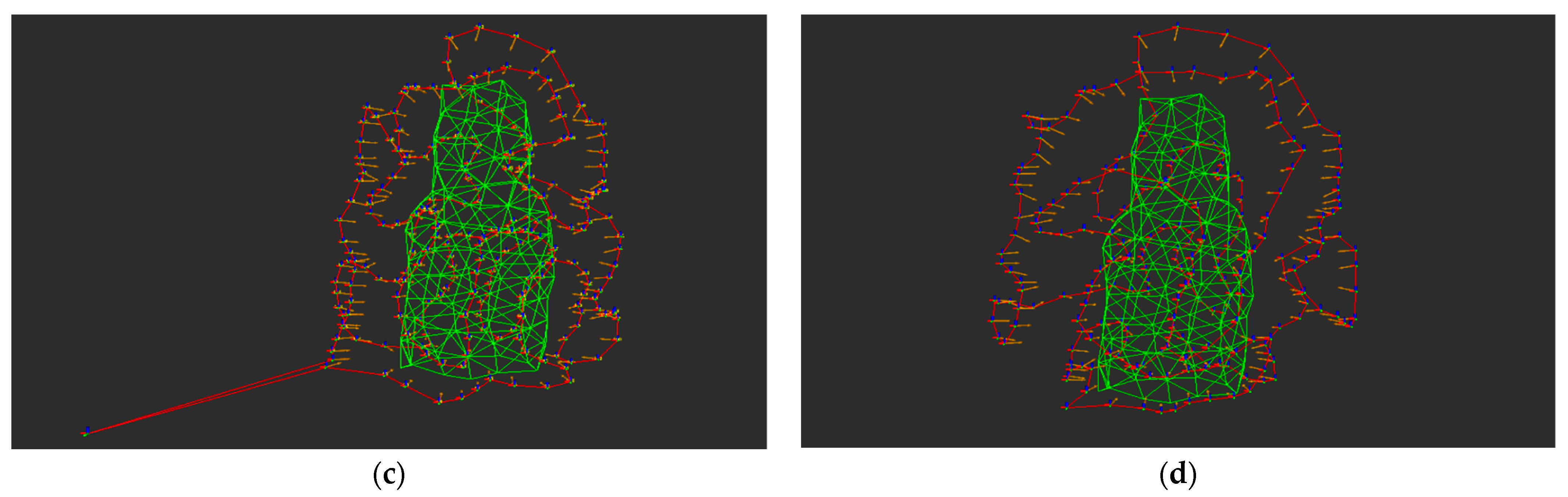
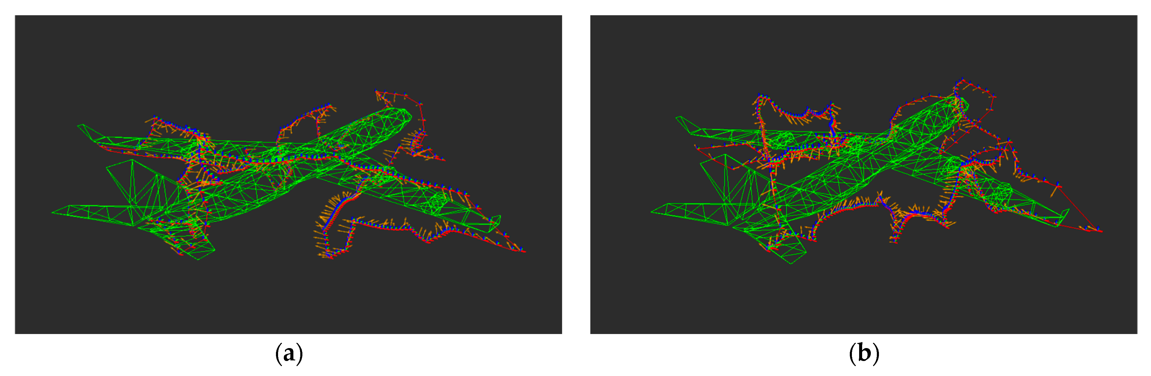
4. Simulation and Evaluation

4.1. Simulation Setup

All simulations in this paper were conducted on the following hardware: Intel(R) Core(TM) i7-13400F processor, NVIDIA GeForce RTX 3070 graphics card, 32GB RAM. To evaluate the proposed algorithm, simulations were performed on Ubuntu 18.04 using Robot Operating System (ROS) melodic, and RVIZ was employed for visualization. We conducted simulations on three different 3D structures: (1) a complex large-scale 3D model of a civil aircraft, (2) a simple small-scale 3D model, hoaHakanaia, and (3) a 3D wind turbine model with a tall height and a dense triangle mesh. These models represent different shapes, levels of complexity, and narrow space characteristics.

Table 1. Different 3D structure models and parameters.

Model
Name	Civil Aircraft	Hoa Hakanaia	Wind Turbine
Number of surface triangles	435	225	720
Dimensions (m)	63.6 × 60.3 × 16.7	8.4 × 5.2 × 19.5	60.7 × 10.3 × 108.5

shows the shapes and parameters of the models used.

4.2. Comparative Methods and Evaluation Metric

4.2.1. Comparative Methods

We compared our QECI-CPP method with the Structural Inspection Planner (SIP) [18], co-optimal coverage path planning (CCPP) [20], and LKH-based TSP using Improved RRT* (IRRT*-LKH) [35]. In SIP, a set of viewpoints was generated by solving an Art Gallery Problem (AGP), and an alternating two-step optimization paradigm was used to find new viewpoints and iteratively optimize the path. The roll and pitch angles of the UAV were considered to be near zero during the path planning computation process, and the camera was mounted on the UAV with a fixed pitch angle. In CCPP, the viewpoint generation and path optimization algorithm use a PSO framework, iteratively optimizing the coverage path without discretizing the motion space or simplifying the perception model like similar methods. $\mathbb{N}$ particles in population were used, and another weight parameter $\epsilon$ is needed. In IRRT*-LKH, an improved path planning algorithm for UAV based on RRT* is proposed. In order to obtain a higher-quality path, considering the optimization effect of the basic path, two random trees are extended from the initial point and the target point, and the deviation around the generated path is sampled during the operation of the algorithm.

Parameter tuning for each method is presented in detail subsequently. All parameters can be categorized into three types: model parameters, such as ${\theta }_h$, ${\theta }_v$, ${\theta }_{min}$, and ${\theta }_{max}$; inspection task requirements, including $d_{min}$, $d_{max}$, and ${\theta }_c$; and algorithm-specific parameters, which are unique to each algorithm. For all algorithms, the model parameters and inspection task requirements remain the same. However, the SIP algorithm has specific requirements, as it is designed for scenarios where the gimbal’s pitch angle is fixed. Therefore, the gimbal’s pitch angle is set to the default value of −25° as specified in the original algorithm [18]. We will now provide a detailed explanation of the selection of the third category of parameters. The parameters unique to our method include $h_l$, $d_{l\_max}$, $d_{l\_min}$, and ${\beta }_w$. Three of these parameters are designed specifically for inspection models in narrow spaces. For example, for an aircraft model, $h_l$, $d_{l\_max}$, and $d_{l\_min}$ are determined by the space height of the fuselage and the maximum and minimum feasible shooting distances within a narrow space. The weight factor ${\beta }_w=1$ is set to balance the inspection quality and efficiency equally. Compared to our algorithm, SIP does not have additional specific parameters. For the CCPP method, the unique parameters include $\epsilon$, $\kappa$, and $\mathbb{N}$. Here, $\epsilon =0.5$ is set to balance shooting quality and distance similarly to our method. As stated in [20], both population size and iteration number positively affect the optimization results, though their effects vary depending on the geometry being inspected. Generally, strong results are obtained with both the population size and iteration number set to 30. Therefore, we also let $\kappa =30$ and $\mathbb{N}=30$ in this paper. To evaluate IRRT*-LKH, we use the viewpoint space described in Section 3.2, with random sampling of viewpoint positions and without additional iterative optimization. The parameters of IRRT* are consistent with [35]. All the above parameters are shown in

Table 2. Parameters for the civil aircraft (distance unit in meters).

$[{\theta }_{min},{\theta }_{max}]$

$[{\theta }_h,{\theta }_v]$

${\theta }_c$

$h_l$

$h_f$

$d_{l\_min}$

$d_{l\_max}$

$d_{min}$

$d_{max}$

${\beta }_w$

$\kappa$

$\epsilon$

$\mathbb{N}$

QECI-CPP

[−90°, 80°]

[120°, 80°]

60°

5.2

0.6

0.5

3

2.5

8

1

30

\

\

SIP

−25°

[120°, 80°]

60°

\

2.5

8

\

30

\

\

CCPP

[−90°, 80°]

[120°, 80°]

60°

\

2.5

8

\

30

0.5

30

IRRT*-LKH

[−90°, 80°]

[120°, 80°]

60°

\

2.5

8

\

\

\

\

,

Table 3. Parameters for hoa hakanaia (distance unit in meters).

	$[{\theta }_{min},{\theta }_{max}]$	$[{\theta }_h,{\theta }_v]$	${\theta }_c$	$h_f$	$d_{min}$	$d_{max}$	${\beta }_w$	$\kappa$	$\epsilon$	$\mathbb{N}$
QECI-CPP	[−90°, 80°]	[120°, 80°]	60°	0.6	1.5	7	1	30	\	\
SIP	−25°	[120°, 80°]	60°	\	1.5	7	\	30	\	\
CCPP	[−90°, 80°]	[120°, 80°]	60°	\	1.5	7	\	30	0.5	30
IRRT*-LKH	[−90°, 80°]	[120°, 80°]	60°	\	1.5	7	\	\	\	\

and

Table 4. Parameters for wind turbine (distance unit in meters).

	$[{\theta }_{min},{\theta }_{max}]$	$[{\theta }_h,{\theta }_v]$	${\theta }_c$	$h_f$	$d_{min}$	$d_{max}$	${\beta }_w$	$\kappa$	$\epsilon$	$\mathbb{N}$
QECI-CPP	[−90°, 80°]	[120°, 80°]	60°	0.6	1.5	13	1	30	\	\
SIP	−25°	[120°, 80°]	60°	\	1.5	13	\	30	\	\
CCPP	[−90°, 80°]	[120°, 80°]	60°	\	1.5	13	\	30	0.5	30
IRRT*-LKH	[−90°, 80°]	[120°, 80°]	60°	\	1.5	13	\	\	\	\

.

The additional key parameter settings for the LKH, RRT*, and VPSolver algorithms in QECI-CPP, as well as for the LKH in IRRT*-LKH, are aligned with those used in the open-source code of the SIP algorithm [36] to ensure fairness in the comparison. The main parameters of the LKH are as follows: the move type used in the local search is specified by MOVE_TYPE = 5, the number of iterations for path calculations is RUNS = 10, the use of sub-gradient optimization is indicated by SUBGRADIENT = 1, the maximum number of candidate edges associated with each node is MAX_CANDIDATES = 5, and the internal precision of the transformation distance is PRECISION = 100. The key parameters of the RRT* are as follows: the size of RRT* space is set to rrt_scope = 25, the number of iterations for the RRT* planner when no connection can be established is rrt_it = 50, the collision check interval is specified by discretization_step = 0.1, and the depth of the recursive obstacle avoidance search is set to max_obstacle_depth = 3.

4.2.2. Evaluation Metric

All the methods were evaluated from five aspects: resolution, orthogonality degree, path distance, computation time, and total path cost. For the convenience of separately calculating and statistically analyzing resolution and orthogonality degree, both terms in Equation (20) were normalized. The evaluation metric for resolution, $r_i$, is defined as follows:

$$\begin{array}{c}{r}_i={\displaystyle \frac{{\displaystyle \sum _{j=1}^3(1-\frac{|{\ell }_{ij}-\frac{{\ell }_a+{\ell }_b}{2}|}{\frac{{\ell }_a+{\ell }_b}{2}})}}{3}}\end{array}$$

(22)

The closer $r_i$ is to 1, the better the resolution. The evaluation metric for orthogonality degree is defined as follows:

$${\beta }_i={\displaystyle \frac{(V_i-m_i)\cdot \overrightarrow{a_i}}{\left|\right|V_i-m_i\left|\right|}}$$

(23)

The closer ${\beta }_i$ is to 1, the better the orthogonality degree. For $r_i$ and ${\beta }_i$, the average values corresponding to all surface triangles are used as the final indicators. For path distance, we use the length of the final collision-free path as the metric. Based on (19), the total path cost $ℂ$ is calculated as follows:

$$ℂ={\Sigma }_i^{T_n}{ℂ}_i$$

(24)

4.3. Results and Analysis

In this section, we first conduct comparative simulations and analysis using four methods on different 3D structures under four metrics: resolution, orthogonality degree, path distance, and computation time. Then, for the civil aircraft model, we analyze the impact of different ${\beta }_w$ on the generated final path. Finally, we assess the change in total path cost with the number of iterations under conditions with and without the high-quality initialization (HQI) strategy designed in Section 3.2.

4.3.1. Comparative Simulation Results

Figure 5a–d show the final coverage paths and generated viewpoints for QECI-CPP, SIP, CCPP, and IRRT*-LKH, respectively. In these figures, the green areas represent the surface triangles of the 3D structures to be inspected, the red lines represent the planned paths, the yellow arrows indicate the viewpoint directions, and the colored markers at the tails of the arrows represent the positions of the viewpoints.

Table 5. Path metrics generated by QECI-CPP and other methods (distance unit in meters).

Path Metrics	Civil Aircraft				Hoa Hakanaia				Wind Turbine
	QECI-CPP	SIP	CCPP	IRRT*-LKH	QECI-CPP	SIP	CCPP	IRRT*-LKH	QECI-CPP	SIP	CCPP	IRRT*-LKH
Resolution	0.94	0.35	0.92	0.32	0.96	0.30	0.93	0.28	0.91	0.29	0.90	0.37
Orthogonality degree	0.87	0.32	0.85	0.39	0.87	0.29	0.87	0.31	0.85	0.31	0.87	0.42
Path distance	593.3	529.8	721.5	571.6	223.6	224.7	358.3	343.8	568.3	472.4	671.2	698.5

presents the path metrics generated using QECI-CPP and other methods. In Figure 5 and Table 5, it is evident that compared to other methods, QECI-CPP produces a more effective coverage path for the civil aircraft model. This superiority is reflected in the achieved maximum orthogonality degree of 0.94 and resolution of 0.87. In contrast, SIP offers the shortest path but compromises inspection quality compared to QECI-CPP and CCPP, as SIP does not prioritize image quality during its iterative process. This highlights QECI-CPP’s ability to achieve superior inspection quality with minimal path distance sacrifice.

Table 6. Computation time for using QECI-CPP and other methods on civil aircraft.

Methods	View Sampling (s)	At Each Iteration (s)			Total (s)
		LKH Time	Cost Evaluation	Greedy Heuristic + Particles Update
QECI-CPP	1.6	0.28	0.056	\	11.3
SIP	1.9	0.43	0.066	\	16.4
CCPP	15.7	6.39	0.667	5.58	427.9
IRRT*-LKH	4.2	\			8.6

displays the computation times for QECI-CPP and other methods applied to the civil aircraft model. For the civil aircraft model, Table 6 indicates that QECI-CPP’s computation time is 11.3 s, compared to 427.9 s for CCPP. Thus, QECI-CPP is approximately 97.4% faster. Compared to SIP’s 16.4 s, QECI-CPP is 31.1% faster. IRRT*-LKH, which takes 8.6 s, is faster than QECI-CPP, but again, with a significant compromise in inspection quality.

Comparing Table 5 and Table 6, it is evident that IRRT*-LKH exhibits the shortest computation time at 8.6 s. However, this method achieves this speed by randomly generating viewpoint positions without iterative consideration of viewpoint quality, resulting in poorer final inspection quality. This is reflected in Table 5, where IRRT*-LKH has a low resolution (0.32) and orthogonality degree (0.39), indicating inferior inspection paths compared to other methods. In contrast, CCPP requires significantly more computation time (427.9 s) than the other methods. This is due to its utilization of a PSO framework for path optimization, which incorporates a greedy heuristic algorithm to actively explore the viewpoint search space. The extensive computation is necessary because the algorithm’s complexity grows exponentially with problem size, rendering it inefficient for larger problems. Additionally, Table 5 shows that the path distance generated by CCPP for the civil aircraft is the longest (721.5 m), further indicating inefficiency in path planning. QECI-CPP, on the other hand, strikes a balance between computation time and path quality. With a total computation time of 11.3 s, it is significantly faster than CCPP and slightly faster than SIP (16.4 s).

Similarly, Figure 6a–d and Table 5 depict the final paths and metrics generated by QECI-CPP, SIP, CCPP, and IRRT*-LKH for hoa hakanaia. The computation times for QECI-CPP and other methods are presented in

Table 7. Computation time for using QECI-CPP and other methods on hoa hakanaia.

Methods	View Sampling (s)	At Each Iteration (s)			Total (s)
		LKH Time	Cost Evaluation	Greedy Heuristic + Particles Update
QECI-CPP	0.9	0.15	0.03	\	7.6
SIP	1.4	0.26	0.05	\	9.3
CCPP	9.7	3.91	0.41	2.16	218.2
IRRT*-LKH	2.9	\			6.1

. Compared to the civil aircraft model, hoa hakanaia exhibits a simpler structure and lower geometric complexity, providing more flexibility in selecting high-quality viewpoints. This enhances the retention of viewpoints generated during high-quality initialization, thereby facilitating easier subsequent iterative optimization. Consequently, this enables the generation of more streamlined paths that balance quality and efficiency. In terms of computation time for hoa hakanaia, Table 7 shows that QECI-CPP is significantly faster than CCPP. QECI-CPP takes 7.6 s, while CCPP takes 218.2 s. This means QECI-CPP is approximately 96.5% faster than CCPP. Furthermore, compared to SIP, which takes 9.3 s, QECI-CPP is about 18.3% faster. IRRT*-LKH has the shortest computation time at 6.1 s, making QECI-CPP 24.6% slower than IRRT*-LKH, but this comes with a trade-off in inspection quality. Examining path distances for hoa hakanaia in Table 5, QECI-CPP generates a path distance of 223.6 m, which is shorter than the 358.3 m generated by CCPP. This indicates that QECI-CPP produces a path that is approximately 37.6% shorter than that of CCPP. When compared to SIP’s path distance of 224.7 m, QECI-CPP offers a marginal improvement of 0.5%. IRRT*-LKH, on the other hand, generates a path distance of 343.8 m, making QECI-CPP’s path 34.9% shorter.

According to Table 6 and Table 7, IRRT*-LKH exhibits the shortest computation time, while CCPP requires the longest. SIP and QECI-CPP show relatively shorter computation times, with QECI-CPP proving more efficient than SIP. This efficiency stems from SIP’s initial viewpoint selection via random sampling, which necessitates extensive computation to optimize the UAV’s overall pose iteratively. In contrast, QECI-CPP’s initialization ensures high-quality path requirements with enhanced regularity. Furthermore, QECI-CPP separates calculations for viewpoint positions and directions using onboard gimbal solutions, enhancing efficiency in path generation and viewpoint direction computation.

Figure 7 and

Table 8. Computation time for using QECI-CPP and other methods on wind turbine.

Methods	View Sampling (s)	At Each Iteration (s)			Total (s)
		LKH Time	Cost Evaluation	Greedy Heuristic + Particles Update
QECI-CPP	3.4	0.37	0.06	\	34.9
SIP	4.9	0.63	0.08	\	38.1
CCPP	16.8	8.81	0.83	12.74	647.5
IRRT*-LKH	4.6	\			12.9

showed final paths and computation time for the wind turbine model using QECI-CPP and other methods. The wind turbine model has a considerable height and a relatively narrow cross-section, which poses certain challenges for CPP of UAV, especially when high-quality image coverage is required. In terms of resolution and orthogonality degree, the QECI-CPP method excels in ensuring high-quality image coverage. Its resolution and orthogonality degree are both close to or better than those of the CCPP method, and significantly better than the SIP and IRRT*-LKH methods. The resolution of QECI-CPP is 0.91, which is 213.8% higher than SIP, 145.9% higher than IRRT*-LKH, and slightly higher than CCPP. The orthogonality degree of QECI-CPP is 0.85, which is 174.2% higher than SIP, 102.4% higher than IRRT*-LKH, but a little lower than CCPP. The viewpoint sampling time of QECI-CPP is 3.4 s, which is 30.6% shorter than SIP, 79.8% shorter than CCPP, and slightly (26.1%) shorter than IRRT*-LKH. However, in terms of total computation time, the total computation time of QECI-CPP is 34.9 s, which is 8.4% shorter than SIP, 94.6% shorter than CCPP, but 170.5% longer than IRRT*-LKH. The path distance of QECI-CPP is 568.3 m, which is 20.3% longer than SIP and shorter than CCPP and IRRT*-LKH.

The simulation results for the wind turbine model show that the QECI-CPP method achieves a good balance between image quality and path efficiency. While the path distance is slightly longer than the SIP method, it significantly outperforms SIP in terms of resolution and orthogonality. The SIP method has moderate computation time but performs poorly in image quality, particularly in resolution and orthogonality. The CCPP method, although close to QECI-CPP in image quality, has extremely long computation times, limiting its practicality. The IRRT*-LKH method has the shortest computation time but far inferior image quality compared to the other methods, making it unsuitable for high-quality inspection tasks.

Overall, paths generated by QECI-CPP consistently demonstrate superior inspection quality and efficiency compared to other methods. The method’s advantages are particularly evident in terms of significantly reduced computation times and shorter path distances relative to CCPP, while maintaining a balance between computation efficiency and path quality compared to SIP and IRRT*-LKH. This makes QECI-CPP a highly effective choice for various inspection tasks, offering robust performance across different models.

We have established a general UAV simulation platform based on PX4, ROS, and Gazebo on an Ubuntu 18.04 system. On this simulation platform, we first imported the civil aircraft model from the paper into Gazebo. Then, we imported the UAV (typhoon_h480). The typhoon_h480 is equipped with a gimbal camera and a GPS module, which are used for visual capture and self-positioning, respectively. After exporting viewpoints planned by QECI-CPP, we used the MAVROS (version 1.16.0) package for communication with the Typhoon H480 in MAVLink format. In the offboard mode, the upper computer program publishes desired motion commands, which the underlying controller uses to track the desired motion. The drone’s body movement controls the yaw of the viewpoint attitude, while the gimbal controls the pitch. Together, these mechanisms adjust the viewpoint attitude. The control of the drone body, gimbal attitude, and photography is managed using topics from the PX4-Autopilot [37]. The virtual simulation video has been uploaded to YouTube at the following link: https://youtu.be/7aENGz2din0?si=laOASAHyiqG3VeMU (accessed on 6 August 2024).

4.3.2. Impact Analysis of Weight Coefficient on the Final Path

Figure 8a–f show the final paths after iterative optimization for the civil aircraft model with ${\beta }_w$ values of 0.0, 0.3, 0.6, 1.0, 1.5, and 2.0, respectively.

Table 9. Coverage path metrics for the civil aircraft model with different weight coefficients.

${\mathit{\beta }}_{\mathit{w}}$	Orthogonality Degree	Resolution	Path Distance (m)	Computation Time (s)
0	0.43	0.38	512.9	11.4
0.3	0.62	0.68	549.2	11.3
0.6	0.87	0.79	587.2	11.4
1.0	0.94	0.87	593.3	11.3
1.5	0.95	0.88	634.6	11.5
2.0	0.96	0.88	640.1	11.4

presents the variations in inspection quality, inspection efficiency, and computation time corresponding to different ${\beta }_w$. As depicted in Table 9, an increase in ${\beta }_w$ enhances the emphasis on inspection quality throughout the iterative optimization process. The selection process prioritizes the quality of the inspection path. However, due to constraints in configuration space and available time for viewpoint selection, the orthogonality degree and resolution of inspection quality tend to stabilize, resulting in increased path distance and a gradual decrease in inspection efficiency. Concurrently, the computation time remains approximately 11.4 s, indicating that changes in ${\beta }_w$ do not significantly impact computation time.

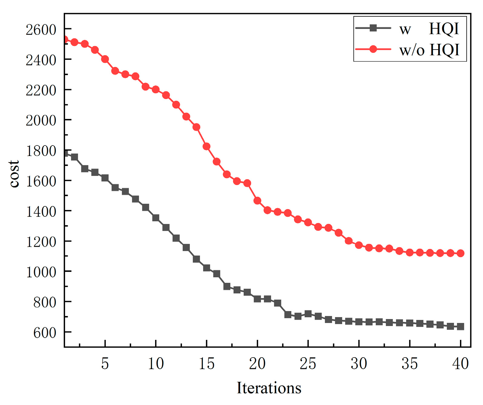
4.3.3. Impact Analysis of HQI on Total Path Cost

Finally, we evaluate the impact of HQI on the total path cost for the two different 3D structures being inspected. Figure 9, Figure 10 and Figure 11 depict the variations in total path cost with the number of iterations under conditions with and without HQI. The results show that without HQI, the path cost tends to increase and is more prone to becoming trapped in local optima.

5. Conclusions

This paper presents the QECI-CPP method, aimed at addressing the CPP problem in high-quality image acquisition for 3D structures. By simultaneously considering inspection quality and efficiency in the objective function, QECI-CPP optimizes inspection quality while maintaining efficiency and significantly reducing computational complexity. Compared with traditional methods, QECI-CPP iteratively optimizes to generate high-quality UAV inspection paths around structures, considering factors such as image resolution, orthogonality degree, and feasible space constraints. This ensures efficient and safe inspections in complex environments while significantly improving computational efficiency through effective initialization and the separation of viewpoint direction calculations. Simulation results demonstrate that QECI-CPP outperforms traditional methods across various 3D structures, achieving high levels of orthogonality and resolution, reducing computation time, and maintaining high path efficiency.

Future work will focus on testing QECI-CPP on real UAV systems to verify its effectiveness in practical applications. Experiments will include the planning of executable trajectories and will account for various model and camera interferences, such as wind disturbance, UAV localization errors, and non-ideal control of the PTU camera. Additionally, we will explore extending the proposed approach to multi-UAV inspection planning in dynamic and uncertain environments.

References

1. Tappe, M.; Dose, D.; Alpen, M.; Horn, J. Autonomous surface inspection of airplanes with unmanned aerial systems. In Proceedings of the 2021 7th International Conference on Automation, Robotics and Applications (ICARA), Prague, Czech Republic, 4–6 February 2021; pp. 135–139. [Google Scholar]
2. Maboudi, M.; Homaei, M.; Song, S.; Malihi, S.; Saadatseresht, M.; Gerke, M. A Review on Viewpoints and Path Planning for UAV-Based 3-D Reconstruction. IEEE J. Sel. Top. Appl. Earth Obs. Remote Sens. 2023, 16, 5026–5048. [Google Scholar] [CrossRef]
3. Ivić, S.; Crnković, B.; Grbčić, L.; Matleković, L. Multi-UAV trajectory planning for 3D visual inspection of complex structures. Autom. Constr. 2023, 147, 104709. [Google Scholar] [CrossRef]
4. Jiao, L.; Peng, Z.; Xi, L.; Ding, S.; Cui, J. Multi-Agent Coverage Path Planning via Proximity Interaction and Cooperation. IEEE Sens. J. 2022, 22, 6196–6207. [Google Scholar] [CrossRef]
5. Tang, Y.; Zhou, R.; Sun, G.; Di, B.; Xiong, R. A Novel Cooperative Path Planning for Multirobot Persistent Coverage in Complex Environments. IEEE Sens. J. 2020, 20, 4485–4495. [Google Scholar] [CrossRef]
6. Yuan, D.; Chang, X.; Li, Z.; He, Z. Learning Adaptive Spatial-Temporal Context-Aware Correlation Filters for UAV Tracking. ACM Trans. Multimed. Comput. Commun. Appl. 2022, 18, 1–18. [Google Scholar] [CrossRef]
7. Höffmann, M.; Patel, S.; Büskens, C. Optimal Coverage Path Planning for Agricultural Vehicles with Curvature Constraints. Agriculture 2023, 13, 2112. [Google Scholar] [CrossRef]
8. Pour Arab, D.; Spisser, M.; Essert, C. Complete coverage path planning for wheeled agricultural robots. J. Field Robot. 2023, 40, 1460–1503. [Google Scholar] [CrossRef]
9. Silberberg, P.; Leishman, R.C. Aircraft inspection by multirotor UAV using coverage path planning. In Proceedings of the 2021 International Conference on Unmanned Aircraft Systems (ICUAS), Athens, Greece, 15–18 June 2021; pp. 575–581. [Google Scholar]
10. Liu, Y.; Dong, J.; Li, Y.; Gong, X.; Wang, J. A UAV-Based Aircraft Surface Defect Inspection System via External Constraints and Deep Learning. IEEE Trans. Instrum. Meas. 2022, 71, 1–15. [Google Scholar] [CrossRef]
11. Wang, H.; Zhang, S.; Zhang, X.; Zhang, X.; Liu, J. Near-Optimal 3-D Visual Coverage for Quadrotor Unmanned Aerial Vehicles Under Photogrammetric Constraints. IEEE Trans. Ind. Electron. 2021, 69, 1694–1704. [Google Scholar] [CrossRef]
12. Saha, A.; Kumar, L.; Sortee, S.; Dhara, B.C. An autonomous aircraft inspection system using collaborative unmanned aerial vehicles. In Proceedings of the 2023 IEEE Aerospace Conference, Big Sky, MT, USA, 4–11 March 2023; pp. 1–10. [Google Scholar]
13. Jing, W.; Polden, J.; Lin, W.; Shimada, K. Sampling-based view planning for 3D visual coverage task with unmanned aerial vehicle. In Proceedings of the 2016 IEEE/RSJ International Conference on Intelligent Robots and Systems (IROS), Daejeon, Republic of Korea, 9–14 October 2016; pp. 1808–1815. [Google Scholar]
14. Englot, B.; Hover, F. Sampling-based coverage path planning for inspection of complex structures. In Proceedings of the International Conference on Automated Planning and Scheduling (ICAPS), Atibaia, Brazil, 25–29 June 2012; Volume 22, pp. 29–37. [Google Scholar]
15. Englot, B.; Hover, F. Planning complex inspection tasks using redundant roadmaps. In Robotics Research: The 15th International Symposium ISRR; Springer International Publishing: Berlin/Heidelberg, Germany, 2017; pp. 327–343. [Google Scholar]
16. LaValle, S.M. Rapidly-Exploring Random Trees: A New Tool for Path Planning. 1998. Available online: http://lavalle.pl/papers/Lav98c.pdf (accessed on 9 October 2020).
17. Bircher, A.; Kamel, M.; Alexis, K.; Burri, M.; Oettershagen, P.; Omari, S.; Siegwart, R. Three-dimensional coverage path planning via viewpoint resampling and tour optimization for aerial robots. Auton. Robot. 2016, 40, 1059–1078. [Google Scholar] [CrossRef]
18. Bircher, A.; Alexis, K.; Burri, M.; Oettershagen, P.; Omari, S.; Mantel, T.; Siegwart, R. Structural inspection path planning via iterative viewpoint resampling with application to aerial robotics. In Proceedings of the 2015 IEEE International Conference on Robotics and Automation (ICRA), Seattle, WA, USA, 26–30 May 2015; pp. 6423–6430. [Google Scholar]
19. Alexis, K.; Papachristos, C.; Siegwart, R.; Tzes, A. Uniform coverage structural inspection path-planning for micro aerial vehicles. In Proceedings of the 2015 IEEE International Symposium on Intelligent Control (ISIC), Sydney, Australia, 21–23 September 2015; pp. 59–64. [Google Scholar]
20. Shang, Z.; Bradley, J.; Shen, Z. A co-optimal coverage path planning method for aerial scanning of complex structures. Expert Syst. Appl. 2020, 158, 113535. [Google Scholar] [CrossRef]
21. Almadhoun, R.; Taha, T.; Seneviratne, L.; Dias, J.; Cai, G. GPU accelerated coverage path planning optimized for accuracy in robotic inspection applications. In Proceedings of the 2016 IEEE 59th International Midwest Symposium on Circuits and Systems (MWSCAS), Abu Dhabi, United Arab Emirates, 16–19 October 2016; pp. 1–4. [Google Scholar]
22. Cao, C.; Zhang, J.; Travers, M.; Choset, H. Hierarchical coverage path planning in complex 3D environments. In Proceedings of the 2020 IEEE International Conference on Robotics and Automation (ICRA), Paris, France, 31 May–31 August 2020; pp. 3206–3212. [Google Scholar]
23. Almadhoun, R.; Taha, T.; Gan, D.; Dias, J.; Zweiri, Y.; Seneviratne, L. Coverage path planning with adaptive viewpoint sampling to construct 3D models of complex structures for the purpose of inspection. In Proceedings of the 2018 IEEE/RSJ International Conference on Intelligent Robots and Systems (IROS), Madrid, Spain, 1–5 October 2018; pp. 7047–7054. [Google Scholar]
24. Sun, Y.; Ma, O. Automating Aircraft Scanning for Inspection or 3D Model Creation with a UAV and Optimal Path Planning. Drones 2022, 6, 87. [Google Scholar] [CrossRef]
25. Glorieux, E.; Franciosa, P.; Ceglarek, D. Coverage path planning with targetted viewpoint sampling for robotic free-form surface inspection. Robot. Comput. Manuf. 2020, 61, 101843. [Google Scholar] [CrossRef]
26. Almadhoun, R.; Taha, T.; Dias, J.; Seneviratne, L.; Zweiri, Y. Coverage path planning for complex structures inspection using unmanned aerial vehicle (UAV). In Proceedings of the Intelligent Robotics and Applications: 12th International Conference, ICIRA 2019, Shenyang, China, 8–11 August 2019; Proceedings, Part V 12*; Springer International Publishing: Berlin/Heidelberg, Germany, 2019; pp. 243–266. [Google Scholar]
27. Ibrahim, A.; Golparvar-Fard, M.; El-Rayes, K. Multiobjective Optimization of Reality Capture Plans for Computer Vision–Driven Construction Monitoring with Camera-Equipped UAVs. J. Comput. Civ. Eng. 2022, 36, 04022018. [Google Scholar] [CrossRef]
28. Luo, R.; Xu, J.; Zuo, H. Automated surface defects acquisition system of civil aircraft based on unmanned aerial vehicles. In Proceedings of the 2020 IEEE 2nd International Conference on Civil Aviation Safety and Information Technology (ICCASIT), Weihai, China, 14–16 October 2020; pp. 729–733. [Google Scholar]
29. Cao, Y.; Cheng, X.; Mu, J. Concentrated Coverage Path Planning Algorithm of UAV Formation for Aerial Photography. IEEE Sens. J. 2022, 22, 11098–11111. [Google Scholar] [CrossRef]
30. Cheng, P.; Keller, J.; Kumar, V. Time-optimal UAV trajectory planning for 3D urban structure coverage. In Proceedings of the 2008 IEEE/RSJ International Conference on Intelligent Robots and Systems (IROS), Nice, France, 22–26 September 2008; pp. 2750–2757. [Google Scholar]
31. Ferreau, H.J.; Kirches, C.; Potschka, A.; Bock, H.G.; Diehl, M. qpOASES: A parametric active-set algorithm for quadratic programming. Math. Program. Comput. 2014, 6, 327–363. [Google Scholar] [CrossRef]
32. Helsgaun, K. An effective implementation of the Lin–Kernighan traveling salesman heuristic. Eur. J. Oper. Res. 2000, 126, 106–130. [Google Scholar] [CrossRef]
33. Helsgaun, K. LKH-The LKH Solver. Available online: http://akira.ruc.dk/~keld/research/LKH/ (accessed on 1 November 2022).
34. Karaman, S.; Frazzoli, E. Sampling-based algorithms for optimal motion planning. Int. J. Robot. Res. 2011, 30, 846–894. [Google Scholar] [CrossRef]
35. Chen, J.; Yu, J. An improved path planning algorithm for UAV based on RRT*. In Proceedings of the 2021 4th International Conference on Advanced Electronic Materials, Computers and Software Engineering (AEMCSE), Changsha, China, 26–28 March 2021; pp. 895–898. [Google Scholar]
36. Open-Source Implementation of the SIP Algorithm as a ROS Package. Available online: https://github.com/ethzasl/StructuralInspectionPlanner (accessed on 26 June 2015).
37. Open-Source Implementation of the PX4 Flight Control Software as a ROS Package. Available online: https://github.com/PX4/PX4-Autopilot (accessed on 1 June 2022).
Figure 1. General workflow of QECI-CPP.
Drones 08 00394 g001
Figure 2. Schematic diagram of the size relationship between the target surface and the image.
Drones 08 00394 g002
Figure 3. Schematic diagram of the size relationship between the camera view and the surface triangle.
Drones 08 00394 g003
Figure 4. Schematic diagram of spatial constraints applied to viewpoints.
Drones 08 00394 g004
Figure 5. Final paths generated for civil aircraft using QECI-CPP and other methods: (a) QECI-CPP; (b) SIP; (c) CCPP; and (d) IRRT*-LKH.
Drones 08 00394 g005
Figure 6. Final paths generated for hoa hakanaia using QECI-CPP and other methods: (a) QECI-CPP; (b) SIP; (c) CCPP; and (d) IRRT*-LKH.
Drones 08 00394 g006aDrones 08 00394 g006b
Figure 7. Final paths generated for wind turbine using QECI-CPP and other methods: (a) QECI-CPP; (b) SIP; (c) CCPP; and (d) IRRT*-LKH.
Drones 08 00394 g007
Figure 8. Coverage paths for the civil aircraft model with different weight coefficients: (a) β w = 0.0; (b) β w = 0.3; (c) β w = 0.6; (d) β w = 1.0; (e) β w = 1.5; and (f) β w = 2.0.
Drones 08 00394 g008aDrones 08 00394 g008b
Figure 9. Changes in total path cost with the number of iterations for the civil aircraft model under conditions with and without HQI.
Drones 08 00394 g009
Figure 10. Changes in total path cost with the number of iterations for hoa hakanaia under conditions with and without HQI.
Drones 08 00394 g010
Figure 11. Changes in total path cost with the number of iterations for wind turbine model under conditions with and without HQI.
Drones 08 00394 g011