Atmospheric Aircraft Conceptual Design Based on Multidisciplinary Optimization with Differential Evolution Algorithm and Neural Networks

Abstract

A methodology for selecting rational parameters of atmospheric aircraft during the initial design stages using a differential evolutionary optimization algorithm and numerical mathematical modeling of aerodynamics problems is proposed. The technique involves implementing weight and aerodynamic balance in the main flight modes, considering atmospheric aircraft with one or two lifting surfaces, applying parallel calculations, and auto-generating a three-dimensional geometric model of the aircraft’s appearance based on the optimization results. A method for accelerating the process of optimizing aircraft parameters in terms of takeoff weight by more than three times by introducing an objective function into the set of design variables is proposed and demonstrated. The reliability of mathematical models used in aerodynamics and the accuracy of the objective function calculation considering various constraints are explored. A comprehensive test of the performance and efficiency of the methodology is conducted by solving demonstration problems to optimize more than ten main design parameters for the appearance of two existing heavy-class unmanned aerial vehicles with known characteristics from open sources.

1. Introduction

The growing importance of aviation technology in various fields of human activity today necessitates the development of new, more effective manned and unmanned aerial vehicles (UAVs). A key role in ensuring the competitiveness of newly created models or modifications of existing aircraft is the initial design stages, during which up to three-quarters of the main technical decisions are made. The success of a project as a whole depends on the correctness of these decisions [1,2,3,4,5,6,7].

Traditional methods of aircraft design [1,2,3,4,5,6,7,8] involve a sequential consideration of the problems of aerodynamics, flight dynamics, strength, weight calculations, and several other disciplines. This determines the iterative character of the initial stages of design, requiring the repeated execution of computational approximations in each discipline. Many solutions are based on the experience of the designer and the established traditions within the development team.

The development of high-performance computing technology has enabled the emergence of a new design paradigm called “concurrent design” [9,10,11], which involves the parallel consideration of weight, energy, and aerodynamic efficiency indicators in early design through the use of multidisciplinary optimization (MDO) methods and numerical mathematical modeling. This approach is already being introduced into the practice of designing manned [12,13,14,15,16,17,18] and unmanned aerial vehicles [19,20,21,22,23,24,25,26,27]. The use of MDOs during the initial design stages for UAVs is of particular importance because UAVs currently cover almost the entire variety of existing and possible unusual aerodynamic configurations [28] and require the consideration of a larger number of design variables across various types. The key requirements of the “concurrent design” paradigm for the design methods used are the high accuracy of mathematical models and the quick impact of optimization algorithms, which allow the consideration of a large number of design variables within the limited time available during the initial design stages.

A monograph [29] is a significant milestone in the automation of aircraft design processes. It formulates and solves design problems in terms of nonlinear mathematical programming (NLP), including the problem of selecting the appearance of aircraft of various types and configurations [30].

Several studies on optimizing the appearance of aircraft have employed various search methods, particularly gradient methods [24,25,31]. However, these methods require the calculation of partial derivatives of the objective function, including the refinement of the calculation of the takeoff weight according to the sizing equation at each iteration. An additional difficulty in solving design selection problems is the heterogeneity and discreteness of design variables. For example, hybrid power plants may include a heat engine and an electric motor in various combinations. Therefore, metaheuristic search methods are being developed to solve these problems. In particular, evolutionary methods borrowed from the natural environment are considered the main approaches. Initially, these were relatively simple algorithms and programs that solved combinatorial optimization problems from homogeneous elements, such as the choice of orientation and number of layers of composite material in different parts of the wing skin [32] or the optimization of structural and geometric parameters of complex composite parts [33,34]. At present, algorithms and programs in this area are intensively developed and implemented in the preliminary design of aviation technology [22,35,36]. The primary components of any evolutionary algorithm are the selection of the best solutions and randomization. The selection of the best solutions ensures convergence to the optimal values, and randomization prevents the solutions from getting trapped in local optima and increases the diversity of the solutions. A good combination of these two components typically ensures that overall optimization can be achieved. One of the most commonly used evolutionary algorithms in engineering problems is the differential evolution (DE) algorithm. DE optimizes a problem by maintaining a population of candidate solutions and creating new candidate solutions by combining existing ones according to simple operators. Then, the candidate solution with the best score or aptitude in the optimization problem is maintained. In this way, the optimization problem can be treated as a black box that simply provides a measure of quality given a candidate solution. In addition, DE offers great flexibility to incorporate adaptive methods, use different forms of vector coding, and work with various surrogate methods (especially those based on deep learning models) [37,38,39,40]. Compared to other optimization algorithms, such as simulated annealing (SA) and genetic algorithms (GAs), the differential evolution (DE) algorithm has several outstanding advantages: it has a fast convergence speed due to its efficient search mechanism, and it is simple to implement with fewer sensitive parameters to adjust. In addition, DE maintains population diversity through differential mutation, effectively balancing the exploration of new solutions and the exploitation of known good solutions, thereby reducing the likelihood of getting stuck in local optima. Another notable advantage of DE over other methods is its excellent scalability for high-dimensional problems [41,42,43]. However, the potential of this optimization method in the field of conceptual aircraft design has not been demonstrated in the limited number of publications. For instance, the optimization process does not consider any stability or control constraints [21,24,44], it does not contemplate a whole mission profile [22,23,24,44], it converges to a local minimum [21], and only a single flying-wing aerodynamic configuration has been considered [45].

The purpose of this work is to demonstrate the capabilities of the DE algorithm with certain adaptability in solving multidisciplinary optimization problems of aircraft-type aerial vehicles with many design variables, including structural ones. The use of the DE algorithm and neural networks to optimize the selection of the aircraft wing airfoil is illustrated.

This paper proposes a method for optimizing the technical parameters of aircraft-type unmanned aerial vehicles at the initial stages of design, which allows considering aerodynamic configurations with two loading surfaces, taking into account the main stages of the flight of the aircraft, performing its longitudinal balancing, setting the degree of margin of longitudinal static stability, maintaining weight and energy balance, considering a significant number of design variables, and automatically visualizing the resulting solution in the form of a surface geometric model of the aerodynamic configuration.

The novelty of the proposed method lies in the following:

-

It includes the iterative process of calculating the takeoff mass based on the sizing equation into the general optimization cycle by adapting the differential evolution optimization algorithm to reduce direct calculations of the objective function and increase the performance of the algorithm.

-

It is a method for parameterizing the ratio of two loading surface areas of an aircraft, which allows one not to be limited to a certain aerodynamic design to optimize its geometric parameters and obtain the configuration based on optimization results (flying-wing, normal, tandem, or canard).

2. Methods and Models

2.1. Formulation of the Conceptual Design Problem

The problem of selecting optimal parameters for the appearance of an aircraft-type UAV was considered in terms of NLP, following [7,29,46] and recent works in this field. In its canonical form, the NLP problem is expressed as follows [47]:

$$F\left({\mathit{x}}^{\mathit{o}\mathit{p}\mathit{t}}\right)\le F\left(\mathit{x}\right)\forall \mathit{x}\in \mathsf{\Omega },$$

$$\mathsf{\Omega }=\left\{\mathit{x}:q_j\left(\mathit{x}\right)\le 0,h_k\left(\mathit{x}\right)=0\right\}$$

(1)

where:

F($\mathit{x}$)—objective function;

$\mathit{x}=\left\{x_1,x_2,\dots ,x_n\right\}$—vector of design variables;

${\mathit{x}}^{\mathit{o}\mathit{p}\mathit{t}}$—optimal solution of the problem;

Ω—area of permissible design variables;

q_j($\mathit{x}$) $\le$ 0, j = 1, …, p—constraints in the form of inequalities;

h_k($\mathit{x}$) = 0, k = 1, …, l—constraints in the form of equations;

n, p, l—the number of variables and constraints.

In the proposed methodology, various technical characteristics of UAVs that are of interest to developers can be defined as objective functions. However, due to the complexity of formulating and solving the problem in a general context, the features of the methodology are further illustrated through the task of improving specific technical characteristics, i.e., minimizing the takeoff weight of two existing heavy drones with different aerodynamic configurations: U-40 [48] and MQ-1 [49] (see Figure 1).

2.2. Digital UAV Model

When solving problems using NLP methods, the mathematical model of the optimization objective must answer two questions:

-

What is the value of the objective function at the considered point in the space of the design variables, defined by vector x?

-

Does this point belong to the feasible region of design variables? If not, how should the value of the objective function be penalized or adjusted in minimization problems?

2.2.1. Objective Function

In the considered tasks, the takeoff weight f($\mathit{x}$) = $W_{TO}$ was selected as the objective function. If another indicator, such as energy or transport efficiency, is selected as the objective function, an accurate calculation of the takeoff weight is still necessary. This value forms the basis for aircraft balancing, weight, energy balance, and absolute geometric parameters. The takeoff weight of an aircraft depends on almost all design parameters, which are iteratively determined using the sizing equation-weight balance [50,51].

2.2.2. Constraints

When solving NLP problems, it is convenient to divide restrictions into three groups:

The first group consists of constraints on the maximum and minimum values of the design variables, typically in the form a_i ≤ x_i ≤ b_i. These constraints define the permissible range of values for each variable and are categorized as geometric constraints, regardless of their character. The physical characteristics may include linear, angular, specific wing loads, and other physical characteristics. The second group comprises inequalities in the form q_j(x) ≤ 0. The third group comprises equations in the form h_k(x) = 0. These constraints define the technical requirements for aircraft operation and typically cannot be explicitly expressed through design variables. Special algorithms are employed to assess compliance with these functional constraints, which can be quite complex. Examples include the vortex-lattice method (VLM) in aerodynamics, statistical data, and criteria such as the “Force coefficient” [50] used in weight calculations.

The second and third groups of restrictions are used as follows:

-

UAV equilibrium conditions in the vertical plane with a given static stability margin:

$$h_1(\mathit{x})=C_m(\mathit{x})=0,$$

(2)

$$h_2(\mathit{x})=C_{L\text{\_}\mathit{bal}}(\mathit{x}) - C_L(\mathit{x})=0;$$

(3)

-

The constraint on the maximum lift coefficient:

$$q_1(\mathit{x})=C_L(\mathit{x}) \le C_L^{*};$$

(4)

-

The constraint on the value of the horizontal tail volume coefficient to ensure the required characteristics of UAV controllability, influencing the size of the horizontal tail arm and its relative area:

$$q_2\left(\mathit{x}\right)=c_{HT}\left(\mathit{x}\right) \in [c_{HT\_min}, c_{HT\_max}]$$

(5)

Here: C_m—the pitch moment coefficient relative to the center mass; C_L—the lift coefficient; C_{L_bal}—the lift coefficient under the equilibrium condition; $C_L^{*}$—the permissible lift coefficient in a given flight mode; $c_{HT}$—the horizontal tail volume coefficient.

2.2.3. Design Variables

The vector of design variables x includes the geometric and specific energy parameters of the aircraft’s appearance, as well as the kinematic parameters of the considered flight modes.

A feature of this work is the inclusion of the input value (preliminary approximation) of the takeoff mass $W_{TO }^{in}$ into vector x. Based on $W_{TO}^{in}$, the output (refined) value of the takeoff weight $W_{TO }^{out}$ is calculated, and then the value of the objective function $W_{TO }^{+}$ = $W_{TO }^{out}$ + ψ, where ψ is the value of the penalty function that implements the requirements of the constraints. The convergence of the optimization process is ensured when $W_{TO}^{in}$ ≈ $W_{TO}^{out}$ = $W_{TO}^{+}$. For variable $W_{TO}^{in}$, the first index in vector x should be used. Therefore, in this work, the proposed vector x consists of 14 design variables: x = [$W_{TO}^{in}$, AR₁, AR₂, ${\mathsf{\Lambda }}_1$, ${\mathsf{\Lambda }}_2$, ${\lambda }_1$, ${\lambda }_2$, δ₁, ${\overline{L}}_2$, ${\overline{S}}_2$, V, W/S, δ₂, α], where: $W_{TO}^{in}$—the input value of the takeoff weight, [kg]; AR₁, AR₂—the aspect ratio of the forward and aftward lifting surfaces, respectively; ${\mathsf{\Lambda }}_1$, ${\mathsf{\Lambda }}_2$—sweep angles of the leading edges of the forward and aftward lifting surfaces, respectively, [°]; ${\lambda }_1$, ${\lambda }_2$—taper ratios of the forward and aftward lifting surfaces, respectively; δ₁—incidence angle of the forward lifting surface, [°]; ${\overline{L}}_2={\displaystyle \frac{L_2}{\overline{c}}}$—the relative distance between the lifting surfaces; ${\overline{S}}_2={\displaystyle \frac{S_2}{S_1}}$—the relative area of the aftward lifting surface compared to the forward lifting surface; V—the flight speed, [m/s]; and W/S—lift system loading, [kg/m²]. The values of the incidence angle δ₂ of the aftward lifting surface and the angle of attack α of the aircraft are carried out by the balancing algorithm within the general optimization cycle.

An information model for NLP optimization includes tools to calculate an aircraft’s takeoff weight based on design variables and assess compliance with constraints.

2.2.4. Scope and Assumptions

• Scope

The proposed algorithm can be applied to aircraft types limited to the following configurations: flying-wing, normal, canard, and tandem equipped with different types of engines.

• Assumptions

  -

  Aerodynamic characteristics are calculated in subsonic mode, up to Mach number 0.6 due to limitations of the vortex-lattice method for aerodynamics.

  -

  Consider only three main flight modes: climb, cruise, and landing.

  -

  Consider only the aircraft’s longitudinal static stability in determining aerodynamic characteristics and solving the aircraft’s existing equations and constraints.

2.3. Methodology for Selecting the Optimal Parameters of an Aircraft-Type UAV

The proposed method is based on the application of the success-history-based adaptive differential evolution (SHADE) optimization algorithm [52,53,54], utilizing penalty functions [55,56,57], population size reduction methods [58,59,60], and numerical mathematical modeling. The SHADE optimization method involves the transformation of information within populations of individuals.

In the considered problems, an individual represents one of the possible project variants–vector x_s, whose components are specific values of the design variables x_i of the designed aircraft:

$${\mathit{x}}_{\mathit{s}}=[x_1, x_2, \dots x_i, \dots x_n{]}_s, s=1,\dots w$$

where:

${\mathit{x}}_{\mathit{s}}$—the vector design variables of the individual s in the population P_g;

s—index of the individual;

w—number of individuals in the population;

i and n—index and number of design variables in the individual s.

A population P_g is a set of individuals s at an iteration of optimization (generation) g, and includes vectors of individuals ${\mathit{x}}_{\mathit{s}}$:

$${\mathit{P}}_{\mathit{g}}={\left\{{\mathit{x}}_1,{\mathit{x}}_2,\dots {\mathit{x}}_{\mathit{s}},\dots ,{\mathit{x}}_{\mathit{w}}\right\}}_{\mathit{g}}, g=1, \dots , m.$$

where: g—the index of the population.

The methodology of this work is based on the algorithm from [45] but incorporates a new approach with significant improvements that allow the following:

-

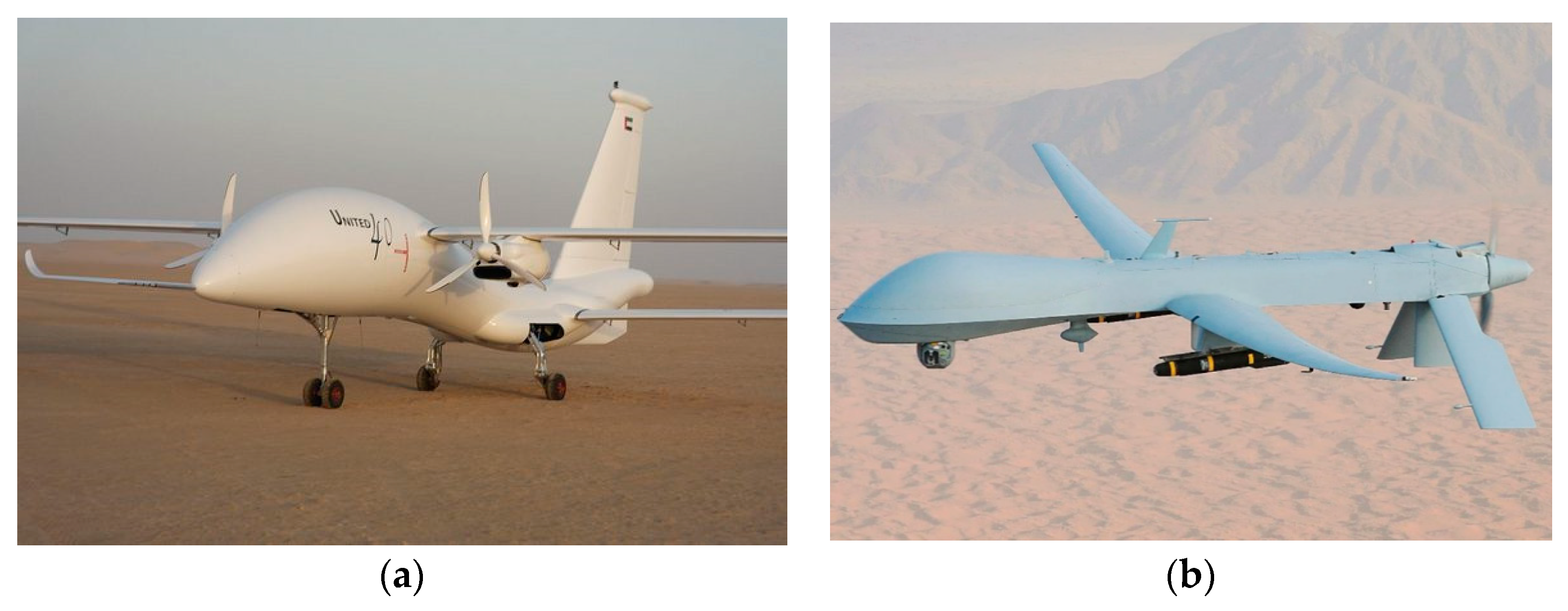
Consideration of various aerodynamic configurations of UAVs with one or two lifting surfaces (flying-wing, normal, canard, tandem);

-

Design of UAVs of different dimensions;

-

Use various types of power plants on UAVs;

-

Increase the performance of calculations through analytical tools and parallel calculations.

The methodology is implemented on the Python platform, integrating the AVL open-source code for aerodynamic calculations [61].

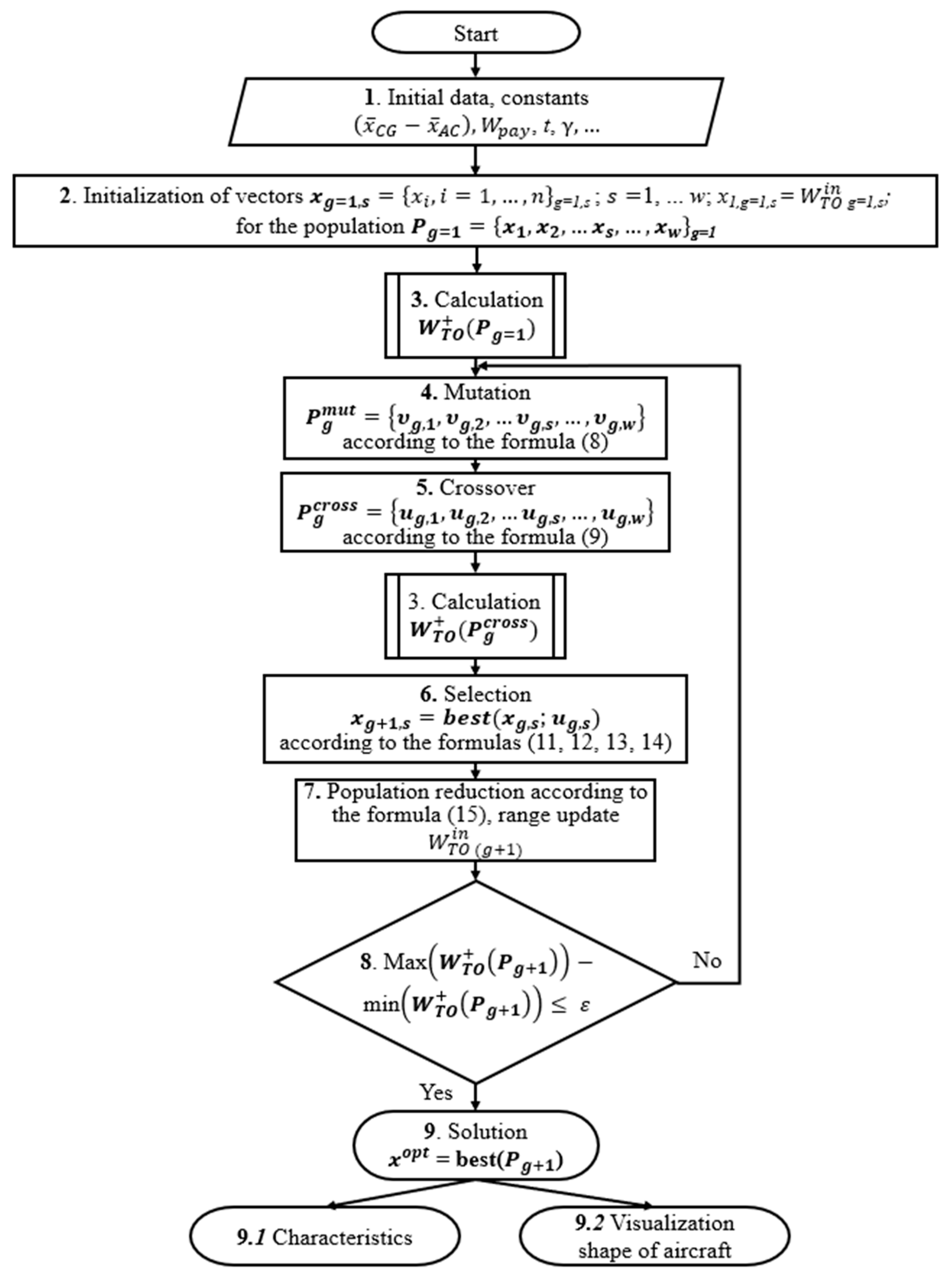
A block scheme of the methodology is presented in Figure 2.

In general, the methodology includes several basic blocks.

• Block 1

The process includes entering initial data and design constants, configuring the optimization method settings, choosing the size of the first w populations, assigning the value of the stop criterion ε, setting the ranges of values for the design variables [x_i(min)… x_i(max)], and defining the constraints q_j ≤ 0. Additionally, it involves specifying the range of possible values for the input takeoff weight of the individuals in the initial approximation at the first iteration [$W_{TOg=1}^{in}$_(min) …$W_{TOg=1}^{in}$_(max)].

• Block 2

The process involves initializing the first population P_g = 1, consisting of vectors ${\mathit{x}}_{\mathit{s}}$ of individuals. The values of the design variables x_g = 1, i in the vectors of each individual x_g = 1, s are selected randomly from the user-defined range of values for the design variables [x_i(min)… x_i(max)] using the Latin hypercube sampling (LHS) method [62]. This includes the initial takeoff weight approximation $W_{TO }^{in}$_g = 1 and s within the given range [$W_{TOg=1}^{in}$_(min) …$W_{TOg=1}^{in}$_(max)]. The size of the first population should be at least w_g = 1 = 10n, where n is the number of design variables.

• Block 3

Block 3 is designed to calculate the values of the objective function $W_{TO }^{+}\left({\mathit{x}}_{\mathit{g},\mathit{s}}\right)$ of individuals ${\mathit{x}}_{\mathit{s}}$ of the population P_g based on the values of their design variables x_i, including the input takeoff weight of the initial approximation $W_{TO }^{in}$_g,s. The value of the objective function of each individual is the output (refined) takeoff weight $W_{TO }^{out}$(x_g,s), calculated using the sizing equation (see Figure 3, Blocks 3.1.s) and supplemented by the value of the penalty ψ (see Figure 3, Block 3.2):

$$W_{TO }^{+}({\mathit{x}}_{\mathit{g},\mathit{s}})=\left\{\begin{array}{cc}{W}_{TO }^{out}\left({\mathit{x}}_{\mathit{g},\mathit{s}}\right)\hfill & if \psi \left({\mathit{x}}_{\mathit{g},\mathit{s}}\right)=0\hfill \\ R\psi \left({\mathit{x}}_{\mathit{g},\mathit{s}}\right)+U^{*}\hfill & if \psi \left({\mathit{x}}_{\mathit{g},\mathit{s}}\right)>0 \bigwedge W_{TO }^{out}\left({\mathit{x}}_{\mathit{g},\mathit{s}}\right)\le U^{*}\hfill \\ R\psi \left({\mathit{x}}_{\mathit{g},\mathit{s}}\right)+W_{TO }^{out}\left({\mathit{x}}_{\mathit{g},\mathit{s}}\right)\hfill & if \psi \left({\mathit{x}}_{\mathit{g},\mathit{s}}\right)>0 \bigwedge W_{TO }^{out}\left({\mathit{x}}_{\mathit{g},\mathit{s}}\right)>U^{*}\hfill \end{array}\right.$$

(6)

where:

$$\psi \left({\mathit{x}}_{\mathit{g},\mathit{s}}\right)={\psi }_1\left({\mathit{x}}_{\mathit{g},\mathit{s}}\right)+{\psi }_2\left({\mathit{x}}_{\mathit{g},\mathit{s}}\right)$$

(7)

$$\begin{gathered} {\psi }_1\left({\mathit{x}}_{\mathit{g},\mathit{s}}\right)=\left\{\begin{array}{c}0 if C_L\left({\mathit{x}}_{\mathit{g},\mathit{s}}\right)\le C_L^{*} \\ C_L\left({\mathit{x}}_{\mathit{g},\mathit{s}}\right)-C_L^{*} if C_L\left({\mathit{x}}_{\mathit{g},\mathit{s}}\right)>C_L^{* } \end{array}\right. \\ {\psi }_2\left({\mathit{x}}_{\mathit{g},\mathit{s}}\right)=\left\{\begin{array}{c}\begin{array}{c}0 if c_{HT}\left({\mathit{x}}_{\mathit{g},\mathit{s}}\right) \left[c_{HT\_min}, c_{HT\_max}\right] \\ c_{HT}\left({\mathit{x}}_{\mathit{g},\mathit{s}}\right)-c_{HT\_max} if c_{HT}\left({\mathit{x}}_{\mathit{g},\mathit{s}}\right)>c_{HT\_max} \end{array}\\ {c_{HT\_min}-c}_{HT}\left({\mathit{x}}_{\mathit{g},\mathit{s}}\right) if c_{HT}\left({\mathit{x}}_{\mathit{g},\mathit{s}}\right)<c_{HT\_min} \end{array}\right. \end{gathered}$$

where $\psi \left(\mathit{x}\right)$—the penalty function; $U^{*}$—the upper limit of the possible takeoff weight; R—the penalty amplification parameter that matches the dimensions and orders of the penalty function with takeoff weight values. Based on the estimates provided in [57], considering the sensitivity of the constraint parameters to the objective function, $U^{*}$= 60,000 and R = 100 were chosen. SHADE is a variation of the DE algorithm that is designed to enhance performance by adapting control parameters. By utilizing historical success rates of different parameter settings, SHADE guides the search process more efficiently. In constrained optimization problems, penalty functions are utilized to handle constraints by transforming them into unconstrained problems. They impose penalties on solutions that violate constraints, steering the search towards feasible regions. In the context of the SHADE optimization algorithm, penalty functions can be integrated to handle constraints by adjusting the objective function value of candidate solutions based on their constraint violations. By doing this, the search process prioritizes feasible solutions while efficiently exploring the solution space.

The result of Block 3 is a vector of objective function values $W_{TO}^{+}\left({\mathit{x}}_{\mathit{g},\mathit{s}}\right)$for each individual x_s in the population P_g (see Figure 3).

The use of the differential evolution method allows the calculation process $W_{TO }^{out}$(x_g,s) to be performed using parallel calculations (see Figure 3, Blocks 3.1.s) with the Joblib library [63] to enhance performance, as the design variable vectors of each individual are independent of one another.

Blocks 4–7 are responsible for the process of generating new populations.

A new population P_g+1 of individuals x_g+1,s at each subsequent step of optimization is formed based on the selection of the best individuals x_g,s from the previous population P_g= {x₁, x₂, … x_s, … x_w}_g and the crossover population ${\mathit{P}}_{\mathit{g}}^{\mathit{c}\mathit{r}\mathit{o}\mathit{s}\mathit{s}}$ = {u₁, u₂, … u_s, … u_w}_g, which is obtained by crossing the population P_g with the mutant population ${\mathit{P}}_{\mathit{g}}^{\mathit{m}\mathit{u}\mathit{t}}$ = {v₁, v₂, …v_s, … v_w}_g.

• Block 4—Mutation

A population ${\mathit{P}}_{\mathit{g}}^{\mathit{m}\mathit{u}\mathit{t}}$ includes mutated vectors of individuals ${\mathit{P}}_{\mathit{g}}^{\mathit{m}\mathit{u}\mathit{t}}$ = {v₁, v₂, … v_s, … v_w}_g, each of which is calculated by the formula:

$${\mathit{v}}_{\mathit{s}}={\mathit{x}}_{\mathit{s}}+F_s\left({\mathit{x}}_{\mathit{p}\mathit{b}\mathit{e}\mathit{s}\mathit{t}}-{\mathit{x}}_{\mathit{s}}\right)+F_s\left({\mathit{x}}_{\mathit{r}1}-{\mathit{x}}_{\mathit{r}2}\right)$$

(8)

where:

${\mathit{x}}_{\mathit{p}\mathit{b}\mathit{e}\mathit{s}\mathit{t}}$—a randomly selected vector from the group of the best vectors of the population P_g. The group of the best vectors is determined based on the principle of minimizing the objective function $W_{TO }^{+}\left({\mathit{x}}_{\mathit{g},\mathit{s}}\right)$, and the size of the group of the best vectors is determined by the algorithm settings [52].

${\mathit{x}}_{\mathit{r}1}$—a random vector from the population P_g, excluding ${\mathit{x}}_{\mathit{s}}$;

${\mathit{x}}_{\mathit{r}2}$—a random vector selected from the combined population P_g and the archive of worst solutions A [52].

The value of the scaling factor F_s is determined by the algorithm settings [52].

• Block 5—Crossover

The vectors u_s = (u₁, u₂, … u_i, … u_n)_s of the crossover population ${\mathit{P}}_{\mathit{g}}^{\mathit{c}\mathit{r}\mathit{o}\mathit{s}\mathit{s}}$ = {u₁, u₂, … u_s, … u_w}_g are formed by crossing the values of mutant vectors v_s = (v₁, v₂, …v_i, … v_n)_s of the mutant population ${\mathit{P}}_{\mathit{g}}^{\mathit{m}\mathit{u}\mathit{t}}$ = {v₁, v₂, …v_s, … v_w}_g with vectors x_s = (x₁, x₂, … x_i, … x_n)_s of the current population P_g = {x₁, x₂, … x_s, … x_w}_g.

Crossing is carried out randomly according to the following conditions:

$$u_{i,s}=\left\{\begin{array}{cc}{v}_{i,s}\hfill & if U\left[\mathrm{0,1}\right]\le {CR}_s or i=i_{rand}\hfill \\ x_{i,s}\hfill & if \mathrm{otherwise}\hfill \end{array}\right.$$

(9)

${CR}_s$—the value of the crossover speed;

$U\left[\mathrm{0,1}\right]$—random number range.

If the new values of the design variables for any individual exceed the specified range after the mutation and crossover operations, they will be reassigned according to the condition:

$$u_i=\left\{\begin{array}{cc}\min \left(x_i\right)\hfill & if u_i<\min \left(x_i\right)\hfill \\ \max \left(x_i\right)\hfill & if u_i>\max \left(x_i\right)\hfill \end{array}\right.$$

(10)

• Block 6—Selection of individuals and the formation of a new population

The values of the objective function $W_{TO}^{+}\left({\mathit{u}}_{\mathit{g},\mathit{s}}\right)$of the crossover vectors u_s are calculated using Block 3 (see Figure 2) and their values are compared with the values of the objective function ${W_{TO}^{+}(\mathit{x}}_{\mathit{g},\mathit{s}})$of the vectors x_s in the current population P_g. The selection of individuals from the new population P_g+1 for the next optimization step is based on the following condition:

$${\mathit{x}}_{\mathit{g}+1,\mathit{s}}=\left\{\begin{array}{cc}{\mathit{u}}_{\mathit{g},\mathit{s}}\hfill & if W_{TO}^{+}\left({\mathit{u}}_{\mathit{g},\mathit{s}}\right)\le W_{TO}^{+}\left({\mathit{x}}_{\mathit{g},\mathit{s}}\right)\hfill \\ {\mathit{x}}_{\mathit{g},\mathit{s}}\hfill & if \mathrm{otherwise}\hfill \end{array}\right.$$

(11)

The objective function, penalty function, and input values of the takeoff weight for each individual will be determined for the new population under the following conditions:

$$W_{TO}^{out}\left({\mathit{x}}_{\mathit{g}+1,\mathit{s}}\right)=\left\{\begin{array}{cc}{W}_{TO}^{out}\left({\mathit{u}}_{\mathit{g},\mathit{s}}\right)\hfill & if W_{TO}^{+}\left({\mathit{u}}_{\mathit{g},\mathit{s}}\right)\le W_{TO}^{+}\left({\mathit{x}}_{\mathit{g},\mathit{s}}\right)\hfill \\ W_{TO}^{out}\left({\mathit{x}}_{\mathit{g},\mathit{s}}\right)\hfill & if \mathrm{otherwise}\hfill \end{array}\right.$$

(12)

$$W_{TO}^{+}\left({\mathit{x}}_{\mathit{g}+1,\mathit{s}}\right)=\left\{\begin{array}{cc}{W}_{TO}^{+}\left({\mathit{u}}_{\mathit{g},\mathit{s}}\right)\hfill & if W_{TO}^{+}\left({\mathit{u}}_{\mathit{g},\mathit{s}}\right)\le W_{TO}^{+}\left({\mathit{x}}_{\mathit{g},\mathit{s}}\right)\hfill \\ W_{TO}^{+}\left({\mathit{x}}_{\mathit{g},\mathit{s}}\right)\hfill & if \mathrm{otherwise}\hfill \end{array}\right.$$

(13)

$$\psi \left({\mathit{x}}_{\mathit{g}+1,\mathit{s}}\right)=\left\{\begin{array}{cc}\psi \left({\mathit{u}}_{\mathit{g},\mathit{s}}\right)\hfill & if W_{TO}^{+}\left({\mathit{u}}_{\mathit{g},\mathit{s}}\right)\le W_{TO}^{+}\left({\mathit{x}}_{\mathit{g},\mathit{s}}\right) \hfill \\ \psi \left({\mathit{x}}_{\mathit{g},\mathit{s}}\right)\hfill & if \mathrm{otherwise}\hfill \end{array}\right.$$

(14)

At this stage, an archive of the worst individuals is created, which will be utilized for mutation in subsequent optimization iterations:

$${\mathit{A}}_{\mathit{g}+1}=\mathit{A}+{\mathit{x}}_{\mathit{g},\mathit{s}} if W_{TO}^{+}\left({\mathit{u}}_{\mathit{g},\mathit{s}}\right)\le W_{TO}^{+}\left({\mathit{x}}_{\mathit{g},\mathit{s}}\right)$$

In this case, a set of vectors representing individuals is formed, with the value of the penalty function equal to zero (ψ = 0) according to the following condition:

$${\mathit{Mxf}}_{\mathit{g}}=\mathit{Ø} +{\mathit{x}}_{\mathit{g}+1,\mathit{s}} if \psi \left({\mathit{x}}_{\mathit{g}+1,\mathit{s}}\right)=0$$

• Block 7—Population reduction and convergence of the sizing equation

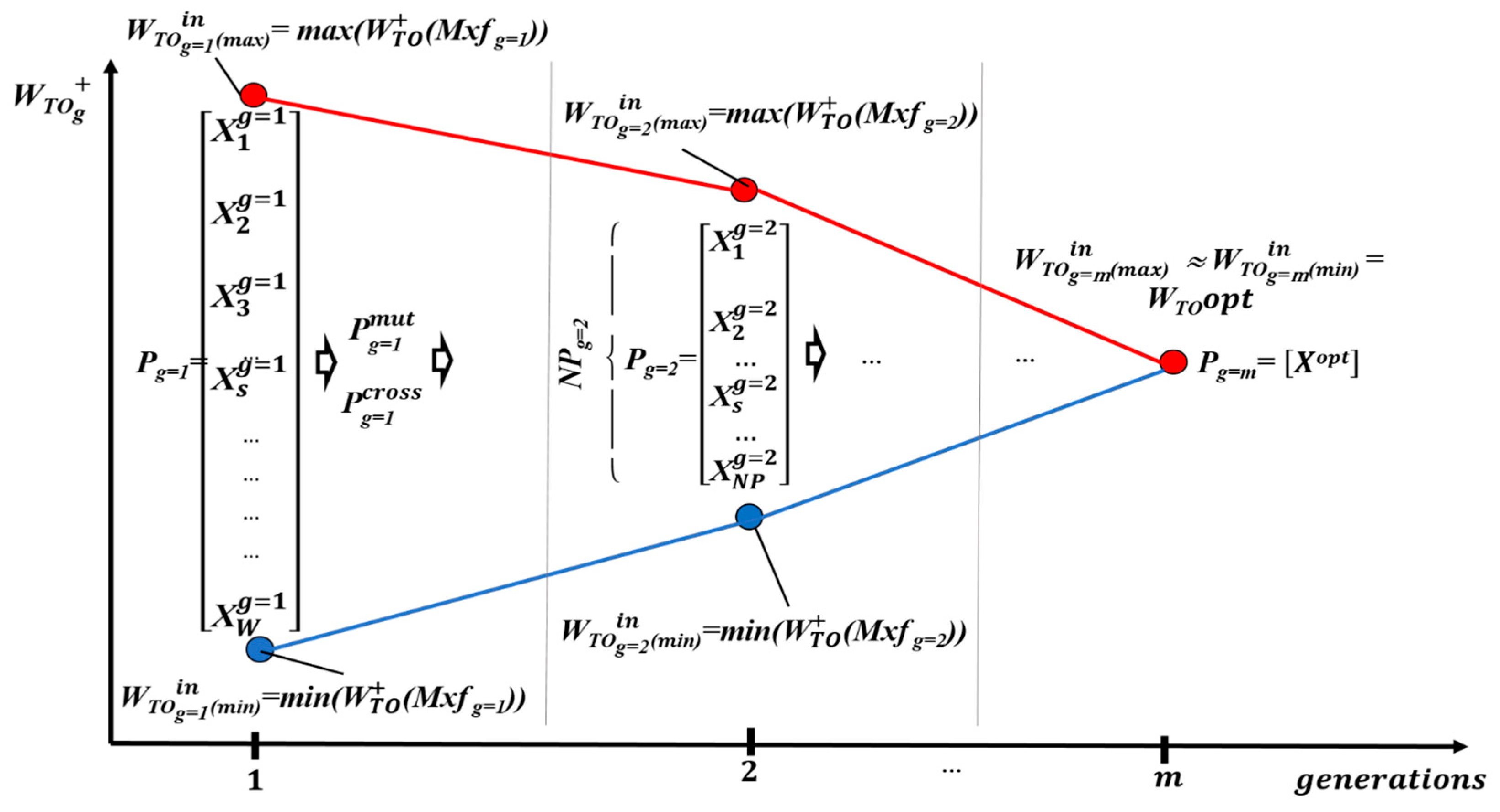
The convergence of the sizing equation is ensured by narrowing the range of values [$W_{TO}^{in}$_(min) …$W_{TO}^{in}$_(max)] at each subsequent optimization step, according to the condition:

$${W_{TOg+1}^{in}}_{\left(\min \right)}=\min \left(\mathit{M}\mathit{x}{\mathit{f}}_{\mathit{g}}\right)$$

$${W_{TOg+1}^{in}}_{\left(\max \right)}=\max \left(\mathit{M}\mathit{x}{\mathit{f}}_{\mathit{g}}\right)$$

That is, the new boundaries [$W_{TOg+1}^{in}$_{(min) …}$W_{TOg+1}^{in}$_(max)] for the next generation are determined based on the most successful individuals (ψ = 0).

If the set of individuals with ψ = 0 at the previous optimization step is empty Mxf_g = ∅ (that is, all $\psi \left({\mathit{x}}_{\mathit{g},\mathit{s}}\right)$ > 0), then the new range of values [$W_{TO}^{in}$_(min) …$W_{TO}^{in}$_(max)] remains the same as in the previous generation:

$${W_{TOg+1}^{in}}_{\left(\min \right)}={W_{TOg}^{in}}_{\left(\min \right)}$$

$${W_{TOg+1}^{in}}_{\left(\max \right)}={W_{TOg}^{in}}_{\left(\max \right)}$$

Each optimization step reduces the population size by excluding the worst individuals with the highest values of the objective function $W_{TO}^{+}$ (ψ >> 0). The population size for the next generation is determined using an exponential population size reduction method:

$${NP}_{g+1}=round\left[{NP}_0{\left({\displaystyle \frac{{NP}_{min}}{{NP}_0}}\right)}^{{\displaystyle \frac{NFE}{{NFE}_{max}}}}\right]$$

(15)

where: NP_min—the minimum population, NP₀—the initial population, NFE_max—the maximum number of evaluated functions, NFE is the current number of evaluated functions. The NP_g+1 individuals with the best fitness are selected.

If the size of the new population is greater than the number of individuals with ψ = 0, then the population will be supplemented by individuals with the lowest values of the objective function among those with ψ ≠ 0.

The initial value of the takeoff weight for the next approximation $W_{TOg+1, s}^{in}$for any individual is a result of the mutation and crossover process of the population from the previous step. If these actions cause the initial takeoff weight $W_{TOg+1, s}^{in}$of an individual in the new generation to exceed the boundaries of the new range [$W_{TOg+1}^{in}$_(min)…$W_{TOg+1}^{in}$_(max)], then this individual will be assigned the nearest boundary value from this range.

Therefore, individuals with ψ ≠ 0 will gradually be eliminated according to the population reduction, and the boundaries [$W_{TO}^{in}$_{(min) …}$W_{TO}^{in}$_(max)] will narrow until the convergence of the sizing equation $W_{TO}^{in}$ ≈ $W_{TO}^{out}$ = $W_{TO}^{+},$ along with the convergence of the overall optimization process max$\left({\mathit{W}}_{\mathit{T}\mathit{O}}^{+}\left({\mathit{P}}_{\mathit{g}+1}\right)\right)$—min$\left({\mathit{W}}_{\mathit{T}\mathit{O}}^{+}\left({\mathit{P}}_{\mathit{g}+1}\right)\right)\le \epsilon$.

The convergence of the objective function when solving the sizing equation is shown schematically in Figure 4.

• Block 8

The convergence condition is evaluated as max$\left({\mathit{W}}_{\mathit{T}\mathit{O}}^{+}\left({\mathit{P}}_{\mathit{g}+1}\right)\right)$ − min$\left({\mathit{W}}_{\mathit{T}\mathit{O}}^{+}\left({\mathit{P}}_{\mathit{g}+1}\right)\right)\le \epsilon$. The algorithm blocks from 3 to 7 will be executed iteratively until convergence is achieved if this condition is not met.

• Block 9

The best individual is selected from the final population ${\mathit{x}}^{\mathit{o}\mathit{p}\mathit{t}},$along with its corresponding objective function $W_{TO}^{+}$(${\mathit{x}}^{\mathit{o}\mathit{p}\mathit{t}}$) (as a result, $W_{TO}^{+}$(${\mathit{x}}^{\mathit{o}\mathit{p}\mathit{t}}$) = ${W_{TO}^{out}}^{opt}$). Additionally, the algorithm yields other output values crucial for comparing results with alternative solutions and for advancing further design stages, including the weights of UAV components, the takeoff weight, flight technical specifications, energy, aerodynamic characteristics, and appearance (see Figure 2, Blocks 9.1–9.2).

The pseudocode of the algorithm (see Figure 2) is presented in Appendix A.

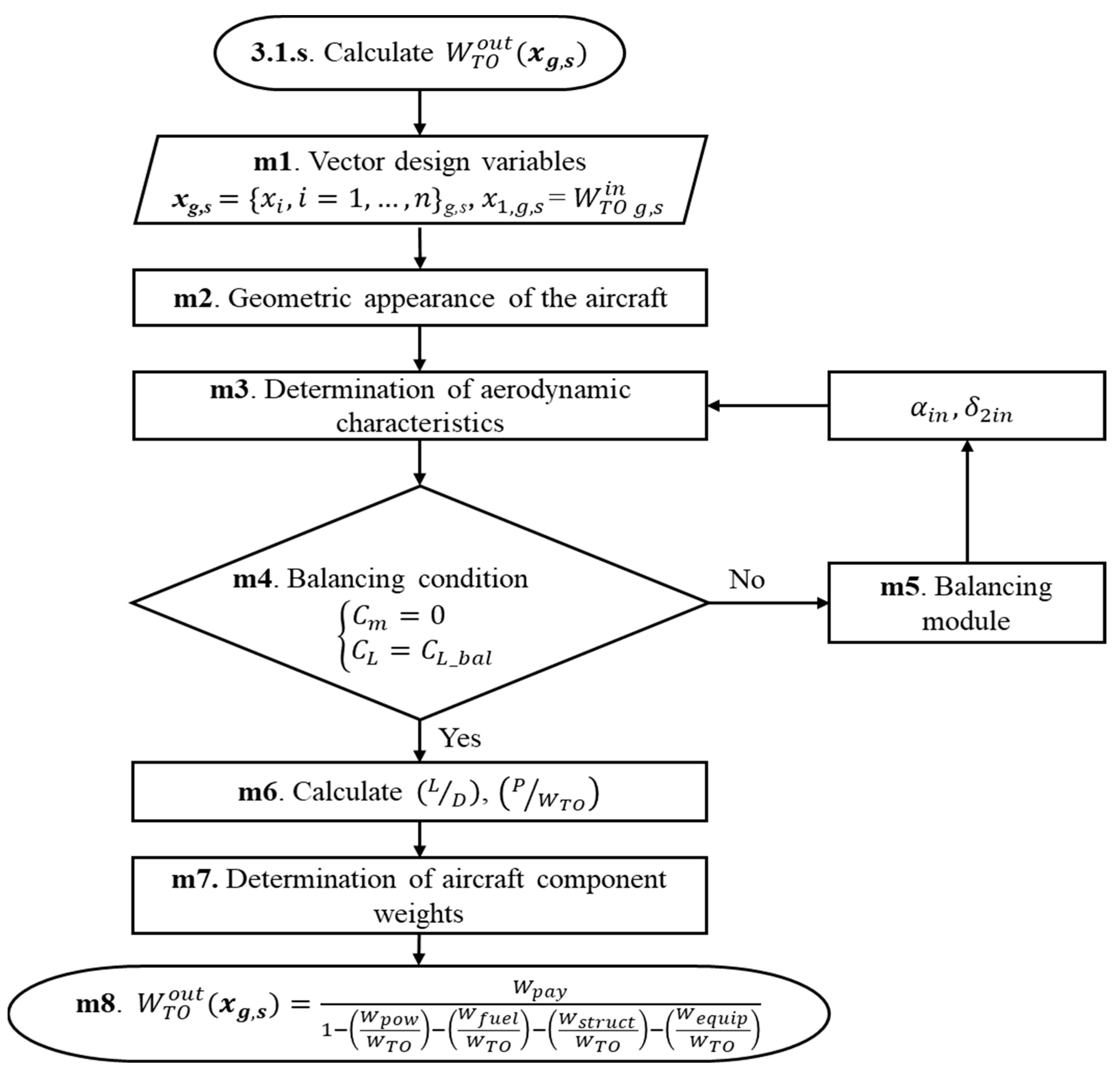
The algorithm for calculating the output (refined) takeoff weight $W_{TO}^{out}$(x_g,s) (see Figure 3, Blocks 3.1.s) is one of the cycles of the general optimization algorithm and is presented in more detail in Figure 5:

Block m1—receives as input the initial data from Block 1 and the vector of the design variables of the individual x_g,s in the generation g, which also includes the initial approximation (input value) of the takeoff weight $W_{TOg,s}^{in}$.

Block m2 is used to calculate the absolute geometric characteristics of the aircraft based on the input value of the takeoff weight $W_{TOg,s}^{in}$and the specific load on the lifting surface (W/S)_g,s, the value of which is in the vector of the design variables of the considered individual x_g,s.

Geometric characteristics are used in the algorithm for the following purposes:

-

Automated generation of three-dimensional geometric models of UAVs;

-

Generation of numerical models for calculating the aerodynamic characteristics of UAVs;

-

Application of engineering formulas for aerodynamics, taking into account compressibility and viscous friction;

-

Calculation of the weight of the UAV airframe structure.

Block m3—calculates the aerodynamic characteristics of the UAV in order to determine the lift-to-drag ratio.

Block m4—checks the balancing condition of the UAV in the vertical plane.

Block m5—implements the process of balancing the UAV by selecting the angle of attack α and the incidence angle δ₂ of the balancing surface, taking into account the specified static margin of longitudinal stability.

Block m6—calculates the required power characteristics of the power plants and the required amount of energy carrier at all stages of the flight.

Block m7—calculates the weights of the main components of the UAV.

Block m8—calculates the output takeoff weight $W_{TO}^{out}\left({\mathit{x}}_{\mathit{g},\mathit{s}}\right)$ using the sizing Equation (16) based on the values of the parameters x_i and the input takeoff weight value ${ W}_{TO g,s}^{in}$.

• Calculation of the weights of aircraft components

Taking into consideration the characteristics of the optimization algorithm, the takeoff weight is calculated using Formula (16) for each individual x_g,s of the current generation g.

$$W_{TO }^{out}\left({\mathit{x}}_{\mathit{g},\mathit{s}}\right)={\displaystyle \frac{W_{pay}}{1-\left(\frac{W_{pow}}{W_{TO}}\right)-\left(\frac{W_{fuel}}{W_{TO}}\right)-\left(\frac{W_{struct}}{W_{TO}}\right)-\left(\frac{W_{equip}}{W_{TO}}\right)}}$$

(16)

where: $W_{pay}$—payload; $\left({\displaystyle \frac{W_{pow}}{W_{TO}}}\right)$—relative weight of the power plants; $\left({\displaystyle \frac{W_{fuel}}{W_{TO}}}\right)$—relative weight of fuel (or $\left({\displaystyle \frac{W_{bat}}{W_{TO}}}\right)$—relative weight of batteries in the case of electric power plants); $\left({\displaystyle \frac{W_{struct}}{W_{TO}}}\right)$—relative weight of structure; $\left({\displaystyle \frac{W_{equip}}{W_{TO}}}\right)$—relative weight of equipment and control.

• Weight of energy carrier

In the case of the use of an internal combustion engine UAV (or other type of fuel engine), the relative weight of the fuel is determined by the formula:

$$\left({\displaystyle \frac{W_{fuel}}{W_{TO}}}\right)=\left({\displaystyle \frac{P}{W_{TO}}}\right)Ct$$

(17)

where: $\left({\displaystyle \frac{P}{W_{TO}}}\right)$—power-to-weight ratio [kW/daN]; C—specific fuel consumption [kg/(kW.h)]; t—the flight endurance [h].

In the case of using an electric motor UAV, the relative weight of the batteries will be equal to:

$${\displaystyle \frac{W_{bat}}{W_{TO}}}={\displaystyle \frac{g\left(\frac{P}{W_{TO}}\right)t}{E{\eta }_{pow}Soc}}$$

(18)

where: ${\eta }_{pow}$—efficiency of the power plants; SoC—the state of charge of the battery; E—the specific energy capacity of the battery [kg/(kW.h)]; and g—the acceleration of gravity [m/s²].

2.

The weight of the power plants

The weight of the power plants includes the weight of the propellers and the engine, along with performance support systems such as the fuel system for internal combustion engines and controllers of electric motors when used as a power unit. The relative weight of the engine is calculated according to the formula:

$$\left({\displaystyle \frac{W_{pow}}{W_{TO}}}\right)=k\left({\displaystyle \frac{P}{W_{TO}}}\right)\gamma$$

(19)

where: k—coefficient that takes into account the increase in the weight of the power plants due to the systems; $\gamma$—the specific weight of the engine.

3.

Weight of structure and on-board equipment

The weight of the UAV airframe structure, which includes the weights of the wing, tail, fuselage, landing gear, and on-board equipment, is determined using weight formulas presented in the specialized literature [2,4,6,7,8].

The values included in the denominator of Equation (16) directly or indirectly depend on the takeoff weight and vice versa. Equation (16) is solved through successive approximations: it starts with the initial approximation of the takeoff weight $W_{TO}^{in}$ as input and produces a refined value $W_{TO}^{out}$ as output. The convergence of the solution (16) is achieved when $W_{TO}^{in}$ ≈ $W_{TO}^{out}$ with a given accuracy. The convergence process of the sizing equation is integrated within the general optimization cycle, which has been detailed earlier.

The pseudocode of the takeoff weight calculation algorithm is presented in Appendix B.

• Geometric characteristics (see Figure 5, Block m2)

The geometric characteristics of each individual x_g,s of the current generation (see Figure 5, Block m2) are calculated using the input value of the takeoff weight $W_{TOg,s}^{in}$, the lift system loading (W/S)_g,s, and other relative geometric parameters from the vector of the individual x_g,s generated by the optimization cycle.

The total area of the lifting surfaces of the UAV S_Σ is determined by the formula:

$$S={\displaystyle \frac{W_{TO}}{(W/S)}}$$

(20)

where: W_TO—takeoff weight [kg] and $W/S$—the lift system loading [daN/m²].

The remaining absolute geometric characteristics of each lifting surface are found by the relationships:

$$S=S_1+S_2$$

(21)

$$b_j=\sqrt{{AR}_j{S}_j}$$

(22)

$$c_{tj}={\displaystyle \frac{2S_j}{b_j\left(1+{\lambda }_j\right)}}$$

(23)

$$c_{rj}={\displaystyle \frac{c_{tj}}{{\lambda }_j}}$$

(24)

$$\overline{c}={\displaystyle \frac{2}{3}}{c}_r{\displaystyle \frac{1+\lambda +{\lambda }^2}{1+\lambda }}$$

(25)

where: S₁—the area of the forward lifting surface [m²]; S₂—the area of the aftward lifting surface [m²]; b—the span [m]; $AR$—aspect ratio; j—the index (j = 1 or 2); c_r—root chord [m]; c_t—tip chord [m]; $\lambda$—taper ratio; $\overline{c}$—the mean aerodynamic chord [m]. The geometric twist $\tau$ is determined by the law of distribution of the incidence angles of the flow sections of the wing.

The geometry of the fuselage is described by relative and absolute parameters: fuselage aspect ratio, ${AR}_{\mathrm{f}}$; aspect ratio of the nose and tail fuselage, ${AR}_{\mathrm{n}}$, ${AR}_{\mathrm{t}}$; equivalent mid-section diameter, $d_{mf}^3$; and loading on mid-section (W/S)_mf.

The scientific novelty of the proposed method lies in the utilization of geometric parameters $S$ and $\overline{S_2}$ = $S_2/S_1$, which enable the consideration of aerodynamic configurations involving one or two lifting surfaces without categorizing them into normal, canard, tandem, or flying-wing. The value $\overline{S_2}$ serves as a variable parameter during optimization. In the case $\overline{S_2}$ < 1, UAV has a normal configuration; in the case $\overline{S_2}$ > 1—canard configuration; if $\overline{S_2}$ ~ 1—tandem; and $\overline{S_2}$ = 0 is the flying-wing or tailless configuration. This approach allows for flexibility in optimizing UAV designs across various aerodynamic configurations.

In this context, the main lifting surface is identified as the forward surface if $S_1$ > $S_2,$ and alternatively, as the aftward surface if $S_1<$ $S_2$. Normalization of aerodynamic coefficients and relative geometric characteristics is conducted relative to the mean aerodynamic chord of the main surface.

• Calculation of the aerodynamic characteristics of the UAV (see Figure 5, Block m3)

The calculation of the aerodynamic characteristics of the UAV (see Figure 5, Block m3) is performed for the specific aerodynamic configuration derived from each individual x_g,s. This includes determining key properties and the inductive component of drag using the VLM method [64,65,66] with the open-source AVL software [61] integrated with Python. Additionally, considerations for the compressibility effects and the calculation of viscous friction forces are addressed using established engineering methods.

The pseudocode for creating a calculation file for AVL and determining aerodynamic characteristics is presented in Appendix C.

The primary objective of the aerodynamics model used is to determine the lift-to-drag ratio during each stage of flight in order to assess the necessary energy characteristics of the power plants and the amount of energy carrier required, determined based on the required power-to-weight ratio at different stages of flight, as outlined in Equation (26).

The lift-to-drag ratio, which determines the energy costs during each stage of flight, is calculated as the ratio of the lift coefficient C_L to the drag coefficient C_D corresponding to the specific flight mode.

The energy balance is provided at each of the stages of flight by the expression:

$$\left({\displaystyle \frac{P}{W_{TO}}}\right)={\displaystyle \frac{V}{{\eta }_{vint}}}{\displaystyle \frac{\raisebox{1ex}{$L$}\!\left/ \!\raisebox{-1ex}{$D$}\right.sin\gamma +cos\gamma }{sin\alpha +\raisebox{1ex}{$L$}\!\left/ \!\raisebox{-1ex}{$D$}\right.cos\alpha }}$$

(26)

where: $\gamma$—flight path angle [°]; α—angle of attack [°]; ${\displaystyle \raisebox{1ex}{$L$}\!\left/ \!\raisebox{-1ex}{$D$}\right.}$—lift-to-drag ratio; V—flight speed [m/s]; ${\eta }_{vint}$—efficiency of the propeller.

• UAV balancing (see Figure 5, Block m4)

The determination of the lift-to-drag ratio and the required energy characteristics of the UAV is conducted under the condition that the UAV is in equilibrium in the vertical plane, ensuring:

$$\left\{\begin{array}{cc}M=0\hfill & \left(a\right)\hfill \\ L=L_{bal}\hfill & \left(b\right)\hfill \\ D=Tcos+Wsin\gamma \hfill & \left(c\right)\hfill \end{array}\right.$$

(27)

where: M—the pitch moment relative to the center mass; L—lift force; $L_{bal}$—lift required for equilibrium along the z_w axis of the wind coordinate frame; D—drag force; T—the thrust of the power plants; and W—the weight of the UAV.

Condition (27) is satisfied based on Equation (26). The forces and moments in (a) and (b) of Equation (27) are more conveniently expressed in terms of coefficients.

The lift coefficient $C_{L\_bal}$ required to ensure equilibrium along the z_w axis is determined by the formula:

$$C_{L\_bal}={\displaystyle \frac{g\left(W/S\right)cos\gamma }{\frac{1}{2}\rho V^2}}$$

(28)

where: g—the acceleration of gravity [m/s²]; ${\displaystyle \raisebox{1ex}{$W$}\!\left/ \!\raisebox{-1ex}{$S$}\right.}$—the lift system loading [kg/m²]; $\gamma$—flight path angle [°]; $\rho$—air density [kg/m³]; V—the flight speed [m/s].

The lift coefficient $C_L$ of the aircraft depends on the angle of attack and the angular arrangement of the lifting surfaces relative to each other. Similarly, the coefficient of pitch moment relative to the center of mass also depends on the chosen static margin of longitudinal stability.

The equilibrium problem (27) is an optimization task aimed at satisfying Equations (27a) and (27b) using two variables:

$$\left\{\begin{array}{cc}{C}_m(\alpha ,{\delta }_2)=0\hfill & \left(a\right)\hfill \\ C_L(\alpha ,{\delta }_2)-C_{L\_bal}=0\hfill & \left(b\right)\hfill \end{array}\right.$$

(29)

where: α—angle of attack [°]; ${\delta }_2$—the incidence angle of the balancing aerodynamic surface [°].

The aerodynamic models utilized establish the linear relationships depicted in (29). Therefore, the proposed approach advocates employing an algorithm that heavily relies on analytical methods to expedite the solution of this problem:

-

The calculation of the coefficients $C_L$ and $C_{mA}$ using the numerical VLM method in AVL software pertains to the leading edge of the mean aerodynamic chord of the main lifting surface. This calculation considers two different combinations of α and ${\delta }_2$.

-

Based on the data obtained, a linear approximation of the analytical dependencies $C_L(\alpha ,{\delta }_2)$ = ${\displaystyle \frac{\partial C_L}{\partial \alpha }}(\alpha -{\alpha }_0+{\delta }_2)$ and $C_{mA}(\alpha ,{\delta }_2)$ = $C_{m0}+{\left({\displaystyle \frac{\partial C_m}{\partial C_L}}\right)}_A{C}_L(\alpha ,{\delta }_2)$ is conducted.

-

The position of the aerodynamic focus is calculated relative to the angle of attack from the leading edge of the mean aerodynamic chord of the main lifting surface: $x_{AC}^{\alpha }=-{\displaystyle \frac{\partial C_m}{\partial C_L}}$ and the required position of the center of mass is calculated to achieve a specific static margin of longitudinal stability: ${\overline{x}}_{AC}+\left({\overline{x}}_{CG}-{\overline{x}}_{AC}\right)$, where $\left({\overline{x}}_{CG}-{\overline{x}}_{AC}\right)$ = Δ—the required static margin of longitudinal stability.

-

The dependence is recalculated $C_{m\_CG}(\alpha ,{\delta }_2)$ relative to the required position of the center mass (see Figure 6):

$$C_{m_{CG}}=C_{m0}+C_L=C_{m0}+{\displaystyle \frac{C_{mA}-C_{m0}}{{\left(\frac{\partial C_m}{\partial C_L}\right)}_A}}$$

(30)

-

Analytical expressions for the two lines obtained by the intersection of the plane $C_L=C_L(\alpha ,{\delta }_2)$ (light green) with the plane $C_L=C_{L\_bal}$ (blue), and the plane $C_{m\_CG}=C_{m\_CG}(\alpha ,{\delta }_2)$ (yellow) with the plane $C_{m\_CG}$ = 0 are determined, solutions (29a) and (29b) are found independently of each other (see Figure 7);

-

The solution of the problem (27) is analytically determined as the point B = (${\alpha }^{*},{\delta }_2^{*}$), which represents the intersection of the two lines $C_L(\alpha ,{\delta }_2)=C_{L\_bal}$ (pink) and $C_{m\_CG}(\alpha ,{\delta }_2)=0$ (red) (see Figure 7).

-

Values $C_L\left({\alpha }^{*},{\delta }_2^{*}\right)$ and $C_{m\_CG}({\alpha }^{*},{\delta }_2^{*})$ are also calculated using the VLM method in AVL software to validate the equilibrium conditions.

The pseudocode of the algorithm is presented in Appendix D.

2.4. Visualization of Optimization Results in the Form of a Planned Projection of the optimal Option and Its Three-Dimensional Model

A file *.xlsx containing all of the geometric parameters of the last generation is saved after the optimization cycle is completed.

An additional module is included at the end of the main optimization program to run the FreeCAD program [67] through the Python subprocess package.

The 3D models are constructed using Python-written macro files. These macro files utilize geometric parameters stored in an *.xlsx file to generate the models, save their images in .png format, automatically close the FreeCAD program upon completion, and place them in the FreeCAD installation folder. By utilizing the “run macro on startup” feature, FreeCAD automatically runs the macro file, allowing the entire process to occur in the background of the system.

2.5. Selection of the Wing Airfoil with a Neural Network

Returning to the condition $C_L^{*}$ used for the optimizing prototypes, the selection of the aircraft’s wing airfoil is mathematically defined as:

$$\begin{gathered} f\left({{\mathit{x}}^{\mathbf{\prime }}}^{\mathit{o}\mathit{p}\mathit{t}}\right)\ge f\left({\mathit{x}}^{\mathbf{\prime }}\right)={\displaystyle \frac{c_l^{1.5}}{c_d}} \forall {\mathit{x}}^{\mathbf{\prime }} \in {\mathsf{\Omega }}_1, \\ {\mathsf{\Omega }}_1=\left\{{\mathit{x}}^{\mathbf{\prime }}: c_l^{*}\left({\mathit{x}}^{\mathbf{\prime }}\right)-c_l\ge 0,y_t\left({\mathit{x}}^{\mathbf{\prime }}\right)-y_{t,min}\ge 0\right\} \end{gathered}$$

(31)

where c_l and c_d are the lift and drag coefficients of the airfoil profile; c_l* is the maximum permissible lift coefficient for the specified flight condition (c_l* = C_L*); y_t is the maximum thickness of the airfoil profile; y_t,min is the minimum allowable value of y_t; ${\mathit{x}}^{\mathbf{\prime }}$ denotes the vector of design parameters. The objective function of maximizing the c_l^1.5/c_d parameter was selected in order to improve the endurance of the aircraft [68,69].

At this point of the research, the design parameters are delimited by the CST (class/shape transformation) parameterization method. This method has the advantages of adjustable design variables and powerful parametric geometric shape design ability and has been widely used in aerodynamic design and optimization processes [70].

In order to evaluate the objective function of (31), the AZTLI-NN [71] neural network is used, which is specifically designed for the design of aerodynamic profiles that provide a large endurance. The architecture of AZTLI-NN is based on the neural network proposed by Wang in [72], a network composed of a multilayer perceptron (MLP) and the decoder of a variational autoencoder (VAE) (see Figure 8). The main difference between the neural network proposed by Wang and AZTLI-NN is that the former is designed for the prediction of physical fields of the profile, while the latter provides the prediction of three graphs of aerodynamic coefficients depending on the angle of attack. The graphs predicted by AZTLI-NN are c_l^1.5/c_d vs. α, c_m vs. α, and c_l vs. α.

This neural network was trained with data obtained from computational fluid dynamics simulations (using the OpenFOAM package). In CFD simulations, a viscous, turbulent, and incompressible flow is considered. Figure 9 shows an example of the performance of AZTLI-NN when performing the aerodynamic coefficient predictions compared to OpenFOAM and a wind tunnel test [73].

To solve the optimization task written in (31), the SHADE algorithm is used in conjunction with AZTLI-NN. Making use of a neural network helps the evolutionary algorithm in reducing the calculation time of the objective functions; in addition, as the neural network provides the graphs of c_l vs. α, the search for c_l* is saved in time.

3. Assessment of the Reliability of Models and Methods

3.1. Validation of Mathematical Models of Aerodynamics

The aerodynamic characteristics of the UAV, based on the specified parameters, are calculated using the VLM method integrated with AVL software, alongside engineering formulas implemented on the Python platform. Validation of these calculations is performed by comparing the results with experimental data obtained using the weight method in the T-3 wind tunnel at Samara University. Details of the experimental setup can be found in [74,75]. The object of the study is a model with geometric characteristics presented in Figure 10.

For validation purposes, the integral aerodynamic coefficients C_D, C_L, and C_m, which depend on the angle of attack, were considered.

Figure 11 presents the results of a comparison of experimental data and calculation results.

The validation results demonstrated a good correspondence between the calculated results using the mathematical models and experimental data. The coefficient of variation in the deviation of the coefficients C_D, C_L, and C_m was found to be 6.8%, 6.1%, and 7.3%, respectively.

3.2. Validation of Models and Algorithm for Calculating the Objective Function

To assess the reliability of the objective function calculation and the characteristics obtained from the takeoff weight calculation cycle, the main characteristics of existing UAVs with known data were computed using the proposed models: U-40 [48] and MQ-1 [49]. Both UAVs are equipped with Rotax 914 engines. Some characteristics of these devices (geometric, kinematic, and specific energy) used in the calculations are given in

Table 1. Calculation results.

Parameters	U-40	Calculation	%	MQ-1	Calculation	%
Takeoff weight [kg]	2000	2055	2.68	1020	1015	0.49
Payload [kg]	600	600	0	204	204	0
Engine weight [kg]	152	150	1.3	76	79	3.9
Fuel weight [kg]	450	458	1.8	302	316	4.4
Empty weight [kg]	950	997	4.7	514	495	3.7
Max engine power [kW]	2 × 84.5	2 × 84.1	0.01	84.5	88.3	4.3
Cruise lift-to-drag ratio	n/a	24.8	-	n/a	23.2	-

.

The convergence of the solution of the sizing equation in the proposed conceptual design methodology is ensured through a comprehensive optimization cycle. Therefore, to solve the sizing equation in a direct one-time calculation of the objective function using initial data from Table 1 and Table 2, a regular iterative cycle is used. This iterative cycle accounts for various flight stages: takeoff, climb, cruise, descent, and landing while considering the UAV’s balance in the vertical plane across all flight modes.

Table 1 shows the results of calculating the objective function—takeoff weight, as well as the weights of empty UAVs, fuel, engines, and their maximum power. Similar characteristics of existing considered UAVs [48,49] are also provided in Table 1 for comparison with the calculated results.

The difference in the results of calculating the takeoff weight, as well as the weights of the main parts of the two existing UAVs using the proposed methodology, did not exceed 3–4%. The estimated required power of the power plants and the actual maximum power of the UAV power plants are in the range of 4–5%. The comparison results from Table 1 provide a sufficient assessment of the accuracy in calculating the key characteristics of the UAV using the proposed methodology, suitable for design purposes.

4. Solving Applied Optimization Problems

Using the proposed optimization methodology, the solution to enhancing the characteristics of two existing UAVs, U-40 and MQ-1, by optimizing several of their key parameters is explored.

These examples use the general problem statement (1) presented in Section 2 and incorporate functional constraints (2)–(5).

The objective function is the takeoff weight $W_{TO}$.

A selection of initial values is drawn from Table 1 and Table 2.

Table 3. Some optimization algorithm settings.

Parameters	Value
Lift coefficient constraint (CL)	<0.6
Constraint of the horizontal tail volume coefficient (cHT)	[0.2…0.6]
Initial value of penalty (U*) [kg]	60,000
Optimization stopping criterion: max$\left({\mathit{W}}_{\mathit{T}\mathit{O}}^{+}\left({\mathit{P}}_{\mathit{g}+1}\right)\right)$ − min$\left({\mathit{W}}_{\mathit{T}\mathit{O}}^{+}\left({\mathit{P}}_{\mathit{g}+1}\right)\right)\le \epsilon$	1
Number of design variables (D)	12
Number of initial population (NP0)	10D
Minimum number of generations	12

presents specific settings for the optimization algorithm.

Table 2. Design constants.

Parameters		U-40	MQ-1
Flight endurance [h]		24	35
Static margin longitudinal stability		−0.1
Specific fuel consumption [kg/(kW.h)]	Climb	0.285
	Cruise	0.27
Flight path angle [°]	Climb	+5
	Cruise	0
	Declimb	−5
Propeller efficiency		0.75
Payload [kg]		600	204
Specific weight engine ${\vartheta }_{en}={\displaystyle \frac{W_{en}.g}{10.N_0}}$ [daN/kW]		0.87

Table 2. Design constants.

Parameters		U-40	MQ-1
Flight endurance [h]		24	35
Static margin longitudinal stability		−0.1
Specific fuel consumption [kg/(kW.h)]	Climb	0.285
	Cruise	0.27
Flight path angle [°]	Climb	+5
	Cruise	0
	Declimb	−5
Propeller efficiency		0.75
Payload [kg]		600	204
Specific weight engine ${\vartheta }_{en}={\displaystyle \frac{W_{en}.g}{10.N_0}}$ [daN/kW]		0.87

The number of individuals in the initial population was 120.

The optimization process achieved convergence after 123 generations and took 62 min on a computer running Windows 10, equipped with an Intel(R) Core i7-6700 processor @ 3.40 GHz and 64 GB of RAM. The last generation comprised 22 individuals. Figure 12 illustrates the convergence of takeoff weight calculations during the optimization process using the algorithm employed.

Changes in the geometric parameters of the considered UAV appearance due to optimization are shown in Figure 13; the prototypes’ appearances are shown in red, while the appearance after optimization is shown in blue.

The figures are automatically generated using the FreeCAD program in Batch mode, which renders the general view of the last population of optimization individuals.

Additionally, to conduct a comparative analysis, the aircraft model with optimized parameters based on the UAV U-40 prototype was constructed using the AVL simulation software (see Figure 14). The results presented in

Table 4. Comparison of aerodynamic characteristics before and after optimization of the UAV U-40 prototype.

Parameters	Prototype	Optimization
Cruise drag coefficient	0.019	0.023
Cruise lift coefficient	0.477	0.59
Cruise lift-to-drag ratio	24.8	26
Cruise angle of attack [°]	1.15	2.8

show an improvement in the aerodynamic characteristics of the aircraft after optimization compared to the prototype.

Table 5. Results of optimization of UAV U-40 and MQ-1 parameters.

	Parameters	Optimization
		Min Value	Max Value	Optimal Value		Initial Values
				U-40	MQ-1	U-40	MQ-1
1	${AR}_1$	4	20	14	7.6	20	19
2	${\mathsf{\Lambda }}_1$ [°]	0	25	2.7	0	1	7.22
3	${\lambda }_1$	0.3	1	0.53	0.34	0.33	0.36
4	${\delta }_1$[°]	0	5	2.5	0	2,5	2.5
5	${AR}_2$	4	20	4	18.7	20	6.75
6	${\mathsf{\Lambda }}_2$ [°]	0	25	0	3	1	0
7	${\lambda }_2$	0.3	1	0.63	0.62	0.33	1
8	${\delta }_2$ [°]	−10	+10	−2.2	−2.0	2.2	−2.62
9	${\overline{L}}_2$	3	8	5.1	4.6	5.55	4.37
10	${\overline{S}}_2$	0.2	5	0.2	4.9	1	0.26
11	α [°]	−10	+10	2.8	5.2	-	-
12	V [m/s]	40	90	50	45	55	47
13	W/S [kg/m2]	20	110	92	75	90	73.2
14	WTO [kg]	500	3000	1667	914	2000	1020

presents the results of the parameter optimization. To visually assess the improvements in the characteristics achieved through optimization, the initial characteristics of the aircraft under consideration are also included in

Table 6. Results of calculating the weight of components and aerodynamic characteristics of the UAV as a result of optimization.

Parameters		U-40			MQ-1
		Initial Values	Optimal Value	$\mathit{\xi }$, %	Initial Values	Optimal Value	$\mathit{\xi }$, %
Takeoff weight [kg]		2000	1667	16.7	1020	914	10.4
Payload [kg]		600	600	0	204	204	0
Equipment weight [kg]		n/a	137	-	n/a	84.1	-
Weights [kg]	forward lifting surface	n/a	181.7	-	n/a	22.4	-
	aftward lifting surface	n/a	25.2	-	n/a	123.4	-
	vertical tail	n/a	13.5	-	n/a	19.6	-
	fuselage	n/a	171.6	-	n/a	77.6	-
	landing gear	n/a	84.1	-	n/a	36.5	-
Engine weight [kg]		152	132	13.2	76	76	0
Fuel weight [kg]		450	313.5	30.3	302	266.6	11.7
Propeller weight [kg]		n/a	8.4	-	n/a	3.8	-
Engine power [kW]		2 × 84.5	2 × 62.9	25.6	1 × 84.5	1 × 80.6	4.6
Relative position of the center mass $\left({\overline{x}}_{CG}={\displaystyle \frac{x_{CG}}{MAC}}\right)$		n/a	0.54	-	n/a	−0.651	-
Cruise lift coefficient		n/a	0.59	-	n/a	0.59	-
Cruise lift-to-drag ratio		n/a	26	-	n/a	24.7	-

.

Figure 15 and Figure 16 show histograms illustrating the distribution of weights among the main components of the UAVs and a comparison of the required engine power before and after optimization.

To better understand the optimization results and their analysis, response surfaces for takeoff weight and aerodynamic quality were constructed from the most influential parameters near the minimum achieved for the U-40 UAV (see Figure 17). To accomplish this, direct calculations of the objective function and aerodynamic quality were performed for the following parameters: specific load on the lifting surface and flight speed. The feasible solution region is shown in color. For the given input data, the best combination of minimizing W_TO = 1671 [kg] and maximizing lift-to-drag ratio L/D = 25.34 corresponds to V = 50 [m/s], W/S = 90 [kg/m²]. The obtained results for the lift-to-drag ratio and aircraft takeoff weight are consistent with the results of the proposed method. This confirms the feasibility of extending the choice of the objective function of the proposed algorithm to the lift-to-drag ratio instead of the takeoff weight.

To evaluate computational performance in the application of parallel computing programs, the DE algorithm is applied to the U-40 prototype without using parallel computing programs. The results obtained from the two methods are compared in

Table 7. Compare computing performance when applying parallel computation.

Parameter	Series Computation	Parallel Computation
WTO [kg]	1669	1667
t [min]	260	62

.

The following design constraints were taken to make the airfoil selection: C_l = 0.59, y_t,min = 11%. For the optimization process, NP₀ = 10 × D (D = 14, number of CST parameters suitable to describe the geometry of a wide variety of profiles [72]), 500 generations, and U* = 0.2 were utilized. The ranges of each design parameter are shown in

Table 8. Design intervals to define the wing airfoil of UAVs.

Parameter	Design Interval	Parameter	Design Interval
Au,0	[0.07, 0.35]	Al,0	[−0.30, −0.05]
Au,1	[0.04, 0.55]	Al,1	[−0.26, 0.05]
Au,2	[0.00, 0.45]	Al,2	[−0.36, 0.05]
Au,3	[0.00, 0.55]	Al,3	[−0.47, 0.05]
Au,4	[0.00, 0.55]	Al,4	[−0.47, 0.05]
Au,5	[0.00, 0.50]	Al,5	[−0.42, 0.10]
Au,6	[−0.01, 0.50]	Al,6	[−0.28, 0.10]

.

The optimization test was performed five times to validate the repeatability of the results provided by the SHADE algorithm in conjunction with the AZTLI-NN network. The five optimal geometries of the airfoils obtained are shown in Figure 18, while the aerodynamic characteristics of each airfoil are shown in

Table 9. Aerodynamic characteristics of the optimized airfoils.

Test	cl1.5/cd	α [°]	ytmax	cd	cm
1	42.7059	3.91	0.1152	0.0106	−0.0341
2	42.7059	3.91	0.1137	0.0106	−0.0376
3	42.7059	3.91	0.1125	0.0106	−0.0341
4	42.7059	3.91	0.1105	0.0106	−0.0359
5	42.7059	3.91	0.1128	0.0106	−0.0324

.

Each test required 65 s of computing time.

As can be seen, the AZTLI-NN neural network, together with the SHADE algorithm, is able to provide consistency in the results and save time in optimization processes.

Table 5 demonstrates that the optimization results led to a reduction in the takeoff weight of the considered UAVs and a decrease in the required power of the power plants.

The proposed optimization method uses takeoff weight as the objective function. Minimizing the takeoff weight of the aircraft is achieved based on two main criteria: maximizing aerodynamic efficiency and minimizing structural weight. From the results shown in Table 4, it can be observed that significant differences lie in the aspect ratio and the relative area of the wings. A higher aspect ratio will reduce induced drag, thereby increasing aerodynamic efficiency; however, this also increases the structural weight. The optimization result is a compromise between these two criteria.

The UAV U-40 was designed with a tandem aerodynamic configuration. Optimization results indicate that the proposed methodology allows for parametric optimization not only of specific aerodynamic layouts but also partially addresses circuit synthesis challenges. In a tandem configuration with equal distribution of areas between the wings, all else being equal, the aircraft tends to exhibit a lower lift-to-drag ratio and a heavier structural weight. This circumstance arises because, in cruising flight mode (the main mode for long-range UAVs), the aftward wing is “underloaded”. In the example considered, with ${\overline{S}}_2$ = 1, the forward wing generates 64% of the lift, while the aftward wing generates 36%. Efforts to load the aftward wing result in a normal or canard configuration. The increase in the weight of the U-40 structure is also associated with the higher aspect ratio of both wings. The proposed algorithm redistributed the aerodynamic load more efficiently, resulting in a transition to a normal configuration with a relative ${\overline{S}}_2$= 0.2. This solution enabled a slight reduction in the aspect ratio of the main wing, thereby decreasing the weight of the wing structure and the UAV as a whole. With an improved lift-to-drag ratio of 3.84% and a reduction in the UAV’s takeoff weight by 16.7%, the required power of the power plants decreased by 25.6%. This would potentially allow the UAV U-40 to replace its existing Rotax 914 engines with lighter options, such as the Rotax 912, further reducing both the weight of the power plants and the overall UAV weight.

The aerodynamic configuration of the UAV MQ-1 was chosen more successfully by the developers. However, the placement of heavy power plants in the rear fuselage shifted the center of mass rearward, which required the wing to be positioned closer to the tail. To maintain the necessary horizontal tail volume coefficient, due to the reduction of the horizontal tail arm, its area had to be increased, and the dynamic characteristics of the UAV in the longitudinal channel worsened.

The proposed algorithm enabled the development of a different configuration—a forward horizontal tail with a smaller area and a longer arm. The forward horizontal tail generates positive lift, partially unloading the wing. Consequently, the wing area was reduced, and the lift-to-drag ratio of the UAV was improved. Overall, this resulted in a 10.4% reduction in takeoff weight and a 4.6% reduction in the required power of the power plants.

5. Conclusions

A methodology for optimizing the appearance of UAVs is proposed. The problem is presented in terms of nonlinear mathematical programming. Specific aspects of the methodology related to the conceptual design of aircraft are illustrated using two real examples of heavy-class UAVs with fundamentally different aerodynamic configurations.

The primary focus of the methodology is to ensure high accuracy in predicting the takeoff weight of an aircraft. For this purpose, the VLM method used in aerodynamic calculations has been validated through our own full-scale wind tunnel experiment. A distinctive feature of the proposed approach is the consideration and assurance of longitudinal balancing within the algorithm for determining takeoff weight. Overall, the accuracy of the mathematical models, algorithms, and programs used in the methodology was verified by a single calculation of the takeoff weight, power-to-weight ratio, and fuel weight of each of the considered UAVs based on their geometric characteristics. The discrepancy between the published main parameters and those obtained through the calculation is within the range of 3–4%.

Estimation of the accuracy of optimization algorithms in complex multidisciplinary technical problems deserves special consideration and, apparently, does not have any general methods except for test functions, test models and specially designed problems with a known optimal solution.

The solution to the optimization problems of the takeoff weight for two UAVs, using 14 design variables with a given payload and flight endurance characteristic of the U-40 and MQ-1, significantly reduced the takeoff weight of these vehicles by making certain changes in appearance and geometric parameters. The obtained results can be considered a test of the reliability and effectiveness of the methodology as a whole.

When developing the methodology, particular attention was paid to its computational efficiency. For this purpose, the optimization algorithm allows for parallel calculation of the takeoff weight of each individual in the population and a one-time calculation of $W_{TO}$ and several other measures. The application of parallel computing using four independent cores shortens the calculation time by four times. Particularly noteworthy are the results of a computational experiment in which the current value of the objective function—takeoff weight—was included as a design variable. Preliminary studies indicate that this measure speeds up the optimization process by approximately three times, achieving equivalent results compared to the traditional method of converging the sizing equation at each optimization step. The analysis of the reasons for this acceleration is of significant scientific interest. Using these accelerations, the time required to obtain a solution with 12 design variables is about one hour on a personal computer with an Intel(R) Core i7-6700 @ 3.40 GHz processor and 64 GB of RAM. Considering the complexity of the multidisciplinary combinatorial problem, this performance seems quite acceptable.

The development of a methodology and software for the conceptual design of UAVs, with the achieved parameters of accuracy and speed, can be considered a significant step towards concurrent design technology.

The proposed methodology, based on the considered examples, demonstrated the potential to develop new competitive models of unmanned aerial vehicles or to improve the characteristics of existing modifications in terms of the required energy of the power plants and the takeoff weight of the device as a whole.

Currently, in this paper, only basic aerodynamic configurations are considered, normal, canard, tandem, and neural networks, and have been applied only in airfoil selection. To further develop this work in the future, other aerodynamic configurations such as twin-fuselage, twin-boom, and V-tail configurations should be considered. Additionally, using neural networks to predict the aerodynamic characteristics of the aircraft in equilibrium problems and determining the lift-to-drag ratio, as a replacement for mathematical models, should also be explored.

A further aspect of developing this work is to consider expanding the selection of objective functions, evaluate optimization results when choosing different objective functions, as well as develop multi-objective function optimization algorithms.

References

1. Komarov, V.A.; Borgest, N.M.; Vislov, I.P.; Vlasov, N.V.; Kozlov, D.M.; Korolkov, O.N.; Mainskov, V.N. Kontseptual’noe Proektirovanie Samoleta [Aircraft Concept Design]; Samara National Research University: Samara, Russia, 2013; ISBN 978-5-7883-0921-7. [Google Scholar]
2. Raymer, D.P. Aircraft Design: A Conceptual Approach, 2nd ed.; American Institute of Aeronautics and Astronautics, Inc.: Washington, DC, USA, 2018; ISBN 0-930403-51-7. [Google Scholar]
3. Nicolai, L.M.; Carichner, G.E. Fundamentals of Aircraft and Airship Design; American Institute of Aeronautics and Astronautics: Columbia, LL, USA, 2010; ISBN 978-1-60086-751-4. [Google Scholar]
4. Torenbeek, E. Advanced Aircraft Design: Conceptual Design, Technology and Optimization of Subsonic Civil Airplanes; Wiley: Hoboken, NJ, USA, 2013; ISBN 978-1-118-56811-8. [Google Scholar]
5. Kroo, I.; Altus, S.; Braun, R.; Gage, P.; Sobieski, I. Multidisciplinary Optimization Methods for Aircraft Preliminary Design. In Proceedings of the 5th Symposium on Multidisciplinary Analysis and Optimization, Panama, FL, USA, 7–9 September 1994; pp. 697–707. [Google Scholar]
6. Badyagin, A.A.; Mukhamedov, F.A. Proektirovanie Legkikh Samoletov [Design of Light Aircraft]; Mashinostroenie Publisher: Moscow, Russia, 1978. [Google Scholar]
7. Eger, S.M.; Mishin, V.F.; Liseytsev, N.K.; Badyagin, A.A.; Rotin, V.E.; Sklyansky, F.I.; Kondrashov, N.A.; Kiselev, V.A.; Fomin, N.A. Proektirovanie Samoletov [Aircraft Design]; Mashinostroenie Publ: Moscow, Russia, 1983. [Google Scholar]
8. Sheinin, V.M.; Kozlovsky, V.I. Vesovoye Proektirovanie i Effektivnost’ Passazhirskikh Samoletov [Weight Design and Efficiency of Passenger Aircraft]; Mashinostroenie Publ: Moscow, Russia, 1977. [Google Scholar]
9. Komarov, V.A. Tochnoe proektirovanie [Concurrent design]. Ontol. Des. 2012, 3, 8–23. [Google Scholar]
10. Weishaar, T.A.; Komarov, V.A. Chelovecheskii faktor v proektirovanii aviatsionnykh konstruktsii [Human Factor in the Design of Aviation Structures]. All-Russ. Sci. Tech. J. Flight 1998, 1, 17–23. [Google Scholar]
11. Komarov, V.A.; Weisshaar, T.A. New Approach to Improving the Aircraft Structural Design process. J. Aircr. 2002, 39, 227–233. [Google Scholar] [CrossRef]
12. Manning, V.M. High Speed Civil Transport Design Using Collaborative Optimization and Approximate Models; Northern Trust Corporation: Chicago, IL, USA, 1997. [Google Scholar]
13. Lukyanov, O. Razrabotka Metodiki Vybora Oblika Gruzovykh Samolotov s Ispol’zovaniyem Mnogodistsiplinarnoy Optimizatsii [Development of a Methodology for Selecting the Shape of Cargo Aircraft Using Multidisciplinary Optimization]. Ph.D. Thesis, Samara National Research University, Samara, Russia, 2019. [Google Scholar]
14. Komarov, V.; Lukyanov, O. Multidisciplinary Optimization of the Cargo Airplane Wing Parameters. All-Russ. Sci.-Tech. J. Polet 2018, 3, 3–15. [Google Scholar]
15. Martins, J.R.R.A.; Kenway, G.; Brooks, T. Multidisciplinary Design Optimization of Aircraft Configurations Part 2: High-Fidelity Aerostructural Optimization; University of Michigan: Ann Arbor, MI, USA, 2016. [Google Scholar]
16. Wunderlich, T.; Dähne, S.; Heinrich, L.; Reimer, L. Multidisciplinary Optimization of an NLF Forward Swept Wing in Combination with Aeroelastic Tailoring Using CFRP. CEAS Aeronaut. J. 2017, 8, 673–690. [Google Scholar] [CrossRef]
17. Sgueglia, A.; Schmollgruber, P.; Bartoli, N.; Benard, E.; Morlier, J.; Jasa, J.; Martins, J.R.R.A.; Hwang, J.T.; Gray, J.S. Multidisciplinary Design Optimization Framework with Coupled Derivative Computation for Hybrid. Aircr. J. Aircr. 2020, 57, 715–729. [Google Scholar] [CrossRef]
18. Leifsson, L. Multidisciplinary Design Optimization of Low-Noise Transport Aircraft [Electronic Resource]. Ph.D. Thesis, Virginia Polytechnic Institute and State University, Blacksburg, VA, USA, 2005. [Google Scholar]
19. Champasak, P.; Panagant, N.; Pholdee, N.; Bureerat, S.; Yildiz, A.R. Self-Adaptive Many-Objective Meta-Heuristic Based on Decomposition for Many-Objective Conceptual Design of a Fixed Wing Unmanned Aerial Vehicle. Aerosp. Sci. Technol. 2020, 100, 105783. [Google Scholar] [CrossRef]
20. Escobar-Ruiz, A.G.; Lopez-Botello, O.; Reyes-Osorio, L.; Zambrano-Robledo, P.; Amezquita-Brooks, L.; Garcia-Salazar, O. Conceptual Design of an Unmanned Fixed-Wing Aerial Vehicle Based on Alternative Energy. Int. J. Aerosp. Eng. 2019, 2019, 8104927. [Google Scholar] [CrossRef]
21. Chung, P.H.; Ma, D.M.; Shiau, J.K. Design, Manufacturing, and Flight Testing of an Experimental Flying Wing UAV. Appl. Sci. 2019, 9, 3043. [Google Scholar] [CrossRef]
22. Boutemedjet, A.; Samardžić, M.; Rebhi, L.; Rajić, Z.; Mouada, T. UAV aerodynamic design involving genetic algorithm and artificial neural network for wing preliminary computation. Aerosp. Sci. Technol. 2019, 84, 464–483. [Google Scholar] [CrossRef]
23. Aksugur, M.; Inalhan, G. Design Methodology of a Hybrid Propulsion Driven Electric Powered Miniature Tailsitter Unmanned Aerial Vehicle. J. Intell. Robot. Syst. 2010, 57, 505–529. [Google Scholar] [CrossRef]
24. Gu, H.; Lyu, X.; Li, Z.; Zhang, F. Coordinate Descent Optimization for Winged-UAV Design. J. Intell. Robot. Syst. 2020, 97, 109–124. [Google Scholar] [CrossRef]
25. Ming, L.; Junqiang, B.; Li, L.; Xiaoxuan, M.; Qian, L.; Bao, C. A gradient-based aero-stealth optimization design method for flying wing aircraft. Aerosp. Sci. Technol. 2019, 92, 156–169. [Google Scholar] [CrossRef]
26. Parada, L.M.A. Conceptual and Preliminary Design of a Long Endurance Electric UAV. Master’s Thesis, University of Lisbon, Lisbon, Portugal, 2016. [Google Scholar]
27. Papageorgiou, A. Design Optimization of Unmanned Aerial Vehicles: A System of Systems Approach. Ph.D. Thesis, Linköping Studies in Science and Technology, Linköping, Sweden, 2019. [Google Scholar]
28. Bowers, P.M. Unconventional Aircraft; Blue Ridge Summit, PA; TAB Books: New York, NY, USA, 1984; 323p. [Google Scholar]
29. Eger, S.M.; Liseytsev, N.K.; Samoilovich, O.S. Osnovyi Avtomatizirovannovo Proektirovaniya Samoletov [Fundamentals of Automated Design of Aircraft]; Mashinostroenie Publ: Moscow, Russia, 1986; 232p. [Google Scholar]
30. Malchevskiy, V.V. Matrichno-Topologicheskii Metod Sinteza i Komponovki Samoleta (Opyt Avtomatizatsii Tvorcheskoy Deyatel’nosti Konstruktora) [Matrix-Topological Method of Synthesis and Aircraft Layout (Experience of Automation of the Designer’s Creative Activity)]; Monograph, Moscow Aviation Institute: Moscow, Russia, 2011; 356p. [Google Scholar]
31. Safavi, E.; Tarkian, M.; Gavel, H.; Ölvander, J. Collaborative Multidisciplinary Design Optimization. A Framework Applied on Aircraft Conceptual System Design. Concurr. Eng. 2015, 23, 236–249. [Google Scholar] [CrossRef]
32. Cherniaev, A.; Komarov, V. Multistep Optimization of Composite Drive Shaft Subject to Strength, Buckling, Vibration and Manufacturing Constraints. Appl. Compos. Mater. 2015, 22, 475–487. [Google Scholar] [CrossRef]
33. Kurkin, E.; Espinosa Barcenas, O.U.; Kishov, E.; Lukyanov, O. Topology Optimization and Efficiency Evaluation of Short-Fiber-Reinforced Composite Structures Considering Anisotropy. Computation 2024, 12, 35. [Google Scholar] [CrossRef]
34. Kurkin, E.; Kishov, E.; Espinosa Barcenas, O.U.; Chertykovtseva, V. Gate Location Optimization of Injection Molded Aerospace Brackets Using Metaheuristic Algorithms. In Proceedings of the 2021 International Scientific and Technical Engine Conference (EC), Samara, Russia, 23–25 June 2021; pp. 1–6. [Google Scholar] [CrossRef]
35. Simanowitsch, D.; Theiss, A.; Sudhi, A.; Badrya, C. Comparison of Gradient-Based and Genetic Algorithms for Laminar Airfoil Shape Optimization. In Proceedings of the AIAA SciTech 2022 Forum, ARC. AIAA Scitech Forum 2022, San Diego, CA, USA, 3–7 January 2022; pp. 1–21, ISBN 978-162410631-6. [Google Scholar] [CrossRef]
36. Zingg, D.W.; Nemec, M.; Pulliam, T.H. A comparative evaluation of genetic and gradient-based algorithms applied to aerodynamic optimization. Eur. J. Comput. Mech. 2008, 17, 2008. [Google Scholar] [CrossRef]
37. Xin-She, Y. Engineering Optimization: A Introduction with Metaheuristic Applications; John Wiley & Sons, Inc.: Hoboken, NJ, USA, 2010; 376p, ISBN 978-0-470-58246-6. [Google Scholar] [CrossRef]
38. Blum, C.; Roli, A. Metaheuristics in combinatorial optimization: Overview and conceptual comparison. ACM Comput. Surv. 2001, 35, 268–308. [Google Scholar] [CrossRef]
39. Almufti, S.M.; Shaban, A.A.; Ali, Z.A.; Ali, R.I.; Fuente, J.A.D. Overview of metaheuristic algorithms. Polaris Glob. J. Sch. Res. Trends 2023, 2, 10–32. [Google Scholar] [CrossRef]
40. Pioquinto, J.G.Q.; Moreno, R.A.F. Methods for increasing the efficiency of the differential evolution algorithm for aerodynamic shape optimization applications. In Proceedings of the XXVI All-Russian Seminar on motion Control and Navigation of Aircraft, Samara, Russia, 14–16 June 2023; pp. 166–171. [Google Scholar]
41. Gonzales, G.V.; Isoldi, L.A.; Rocha, L.A.O.; dos Santos, E.D.; Neto, A.J.S. Comparison between differential evolution and simulated annealing algorithms applied to the constructal design of double-t shaped cavities. In Proceedings of the XXI ENMC—National Meeting on Computational Modeling and IX ECTM—Materials Science and Technology Meeting, Rio de Janeiro, Brazil, 8–11 October 2018. [Google Scholar]
42. Saruhan, H. Differential Evolution and Simulated Annealing Algorithms for Mechanical Systems Design. Eng. Sci. Technol. Int. J. 2014, 17, 131–136. [Google Scholar] [CrossRef]
43. Kurkin, E.; Kishov, E.; Quijada Pioquinto, J.G.; Gavrilov, A.; Chertykovtseva, V. Identification of a mathematical model of elastic-plastic behavior of short-reinforced composite materials using evolutionary algorithms. In Proceedings of the X International Conference on Information Technology and Nanotechnology (ITNT), Samara, Russia, 20–24 May 2024; pp. 1–6. [Google Scholar] [CrossRef]
44. Karakas, H.; Koyuncu, E.; Inalhan, G. ITU Tailless UAV Design. J. Intell. Robot. Syst. Theory Appl. 2013, 69, 131–146. [Google Scholar] [CrossRef]
45. Barcenas, O.U.E.; Pioquinto, J.G.Q.; Kurkina, E.; Lukyanov, O. Multidisciplinary Analysis and Optimization Method for Conceptually Designing of Electric Flying-Wing Unmanned Aerial Vehicles. Drones 2022, 6, 307. [Google Scholar] [CrossRef]
46. Lazarev, I.B. Osnovy Optimal’nogo Proektirovaniya Konstruktsii [Fundamentals of Optimal Design of Structures]; Siberian State Academy of Railway Engineering: Novosibirsk, Russia, 1995; 295p. [Google Scholar]
47. Malkov, V.P.; Ugodchikov, A.G. Optimization of Elastic Systems; Nauka Publ: Moscow, Russia, 1981. [Google Scholar]
48. Srednevysonyi Bespilotnyi Letatel’nyi Apparat Bol’šoi Prodolžiten’nosti Polota United 40 [Medium-Altitude Long-Endurance Unmanned Aerial Vehicle United 40]. Available online: https://vpk.name/library/f/united-40.html (accessed on 2 December 2023).
49. The General Atomics “Predator MQ-1” UAS. Available online: https://barnardmicrosystems.com/UAV/uav_list/predator.html (accessed on 2 December 2023).
50. Bolkhovitinov, V.F. Puti Razvitiya Letatelnykh Apparatov [Ways of Development of Flying Apparatus]; Oborongiz Publ.: Moscow, Russia, 1962; 132p. [Google Scholar]
51. Komarov, V.A. Vesovoy analiz aviatsionnykh konstruktsii: Teoreticheskie osnovy [Weight analysis of aviation structures: Theoretical foundations]. All-Russ. Sci. Tech. J. Flight 2000, 1, 31–39. [Google Scholar]
52. Tanabe, R.; Fukunaga, A. Success-history based parameter adaptation for Differential Evolution. In Proceedings of the 2013 IEEE Congress on Evolutionary Computation, Cancun, Mexico, 20–23 June 2013; pp. 71–78. [Google Scholar] [CrossRef]
53. Jin, R.; Chen, W. An efficient algorithm for constructing optimal design of computer experiments. In Proceedings of the DETC’03 ASME 2003 Design Engineering Technical Conferences and Computers and Information in Engineering Conference, Chicago, IL, USA, 2–6 September 2003. [Google Scholar]
54. Viktorin, A.; Senkerik, R.; Pluhacek, M.; Kadavy, T.; Jasek, R. A Lightweight SHADE-Based Algorithm for Global Optimization—liteSHADE. Lect. Notes Electr. Eng. 2020, 554, 197–206. [Google Scholar] [CrossRef]
55. Storn, R.; Price, K. Differential Evolution—A Simple and Efficient Adaptive Scheme for Global Optimization over Continuous Spaces; Technichcal Report TR-95-012; ICSI: Berkeley, CA, USA, 1995. [Google Scholar]
56. Storn, R.; Price, K. Differential evolution—A Simple and Efficient Heuristic for Global Optimization over Continuous Spaces. J. Glob. Optim. 1997, 11, 341–359. [Google Scholar] [CrossRef]
57. Ali, M.M.; Zhu, W.X. A penalty function-based differential evolution algorithm for constrained global optimization. Comput. Optim. Appl. 2013, 54, 707–739. [Google Scholar] [CrossRef]
58. Pioquinto, J.G.Q.; Shakhov, V.G. Acceleration of Evolutionary Optimization for Airfoils Design with Population Size Reduction Methods. In Proceedings of the 20th International Conference on the Aviation and Cosmonautics, Samara, Russia, 22–26 November 2021; pp. 22–26. [Google Scholar]
59. Wong, I.; Liu, W.; Ho, C.H.; Ding, X. Continuous adaptive population reduction (CAPR) for differential evolution optimization. SLAS Technol. 2017, 22, 289–305. [Google Scholar] [CrossRef] [PubMed]
60. Tanabe, R.; Fukunaga, A.S. Improving the search performance of SHADE using linear population size reduction. In Proceedings of the 2014 IEEE Congress on Evolutionary Computation (CEC), Beijing, China, 6–11 July 2014; pp. 1658–1665. [Google Scholar] [CrossRef]
61. AVL Overview. Available online: https://web.mit.edu/drela/Public/web/avl/ (accessed on 13 October 2023).
62. Viana, F.A. A tutorial on Latin hypercube design of experiments. Qual. Reliab. Eng. Int. 2015, 32, 1975–1985. [Google Scholar] [CrossRef]
63. Sharma, H. Lightweight Pipelining in Python. Using Joblib for Storing the Machine Learning Pipeline to a File. Available online: https://towardsdatascience.com/lightweight-pipelining-in-python-1c7a874794f4 (accessed on 2 November 2023).
64. Belotserkovsky, S.M. Thin Carrying Surface in the Subsonic Flow of Gas; Rozalskaya, N.I., Sh, I., Axelrod, T.D., Eds.; Doverman, Nauka Publisher: Moscow, Russia, 1965; 244p. [Google Scholar]
65. Katz, J.; Plotkin, A. Low-Speed Aerodynamics, 2nd ed.; Cambridge University Press: Cambridge, UK, 2001; 126p. [Google Scholar] [CrossRef]
66. Budziak, K. Aerodynamic Analysis with Athena Vortex Lattice (AVL); Hamburg University of Applied Sciences: Hamburg, Germany, 2015. [Google Scholar]
67. FreeCAD. Available online: https://www.freecad.org/ (accessed on 21 January 2024).
68. Nikolaev, N.V. Optimization of airfoils along high-aspect-ratio wing of long-endurance aircraft in trimmed flight. J. Aerosp. Eng. 2019, 32, 04019090. [Google Scholar] [CrossRef]
69. Quijada Pioquinto, J.Q.; Shakhov, V.; Minaev, E.; Kurkin, E.; Lukyanov, O. Optimization of Airfoils for the Design of Long Endurance Aircrafts Using Deep Learning Models and Metaheuristics Algorithms. Preprints 2024, 2024071992. [Google Scholar] [CrossRef]
70. Kulfan, B.M.; Bussoletti, J.E. “Fundamental” parametric geometry representations for aircraft component shapes. In Proceedings of the 11th AIAA/ISSMO Multidisciplinary Analysis and Optimization Conference, Portsmouth, VA, USA, 6–8 September 2006. [Google Scholar]
71. AZTLI-NN. Available online: https://github.com/OpenVozduj/AZTLI-NN (accessed on 22 July 2024).
72. Wang, J.; He, C.; Li, R.; Chen, H.; Zhai, C.; Zhang, M. Flow field predictions of supercritical airfoils via variational autoencoder based deep learning framework. Phys. Fluids 2021, 33, 086108. [Google Scholar] [CrossRef]
73. Althaus, D.; Wortmann, F.X. Experimental Results from Laminar Wind Tunnel of the Institut fur Aero- und Gasdynamic der Universitat Stuttgart; Fried; Vieweg & Sohn: Stuttgart, Germany, 1981; pp. 1–20. [Google Scholar]
74. Lukyanov, O.E.; Tarasova, E.V.; Martynova, V.A. Udalionoe upravlenie eksperimental’noi ustanovkoi i avtomatizatsia obrabotki eksperimental’nykh dannykh [Remote control of experimental installation and automation of experimental data processing]. Proc. Samara Sci. Cent. Russ. Acad. Sci. 2017, 19, 128–132. [Google Scholar]
75. Lukyanov, O.E.; Martynova, V.A. Eksperimental’nye issledovaniya aerodinamicheskikh kharakteristiki modeli korpusha nesushchey forma [Experimental studies of the aerodynamic characteristics of the model of the hull of the bearing form]. Proc. Samara Sci. Cent. Russ. Acad. Sci. 2016, 18, 83–89. [Google Scholar]
Figure 1. View in the plan of the considered UAV heavy class: (a) U-40; (b) MQ-1.
Drones 08 00388 g001
Figure 2. Block scheme of the algorithm of the proposed methodology for optimizing the design parameters of UAVs.
Drones 08 00388 g002
Figure 3. Block-scheme of calculation for objective function.
Drones 08 00388 g003
Figure 4. Simulation of the convergence process of the objective function.
Drones 08 00388 g004
Figure 5. Block scheme of the takeoff weight calculation algorithm based on the iterative solution of the sizing equation with the UAV balancing cycle in the vertical plane.
Drones 08 00388 g005
Figure 6. Determination of the pitch moment coefficient relative to the center mass.
Drones 08 00388 g006
Figure 7. Solve the balancing problem. (a) Dependence of Cm from α and δ 2 . (b) Dependence of CL from α and δ 2 . (c) Solution of the condition UAV balancing.
Drones 08 00388 g007
Figure 8. Architecture of the AZTLI-NN neural network.
Drones 08 00388 g008
Figure 9. Aerodynamic coefficients of the FX 66-S-161 profile obtained with a laminar wind tunnel [71], with OpenFOAM and AZTLI-NN. (a) cd vs. α, (b) cm vs. α, (c) cl vs. α.
Drones 08 00388 g009
Figure 10. Validation of mathematical models of aerodynamics. (a) Experimental model in a wind tunnel. (b) Geometric parameters of an experimental model in a wind tunnel.
Drones 08 00388 g010
Figure 11. Results of aerodynamic properties. (a) Dependence of CD from α . (b) Dependence of CL from α . (c) Dependence of Cm from α by AVL; ♦ by experiment.
Drones 08 00388 g011
Figure 12. Example of calculating takeoff weight by generations of the proposed algorithm.
Drones 08 00388 g012
Figure 13. Appearance of UAV prototypes (red) and after optimization (blue): (a) U-40; (b) MQ-1.
Drones 08 00388 g013
Figure 14. Modeling of UAV U-40: (a) prototype; (b) optimization.
Drones 08 00388 g014
Figure 15. Weight summary of the design assignment for UAV modernization: (a) U-40; (b) MQ-1.
Drones 08 00388 g015
Figure 16. Comparison engine power of prototypes and after optimization.
Drones 08 00388 g016
Figure 17. Dependence of L/D (a) and WTO (b) on speed and wing loading.
Drones 08 00388 g017
Figure 18. Optimal airfoils for the provided design conditions.
Drones 08 00388 g018