Improved Nonlinear Model Predictive Control Based Fast Trajectory Tracking for a Quadrotor Unmanned Aerial Vehicle

Abstract

This article studies a nonlinear model predictive control (NMPC) scheme for the trajectory tracking efficiency of a quadcopter UAV. A cost function is first proposed that incorporates weighted increments of control forces in each direction, followed by a weighted summation. Furthermore, a contraction constraint for the cost function is introduced based on the numerical convergence of the system for the sampling period of the UAV control force. Then, an NMPC scheme based on improved continuous/generalized minimum residuals (C/GMRES) is proposed to obtain acceptable control performance and reduce computational complexity. The proposed control scheme achieves efficient and smooth tracking control of the UAV while guaranteeing the closed-loop stability of the system. Finally, simulation results are presented to illustrate the effectiveness and superior performance of the proposed NMPC control scheme.

1. Introduction

Recently, unmanned aerial vehicles (UAVs) have aroused great interest and attention in civilian fields, including aerial photography, cargo transportation, and rescue missions [1,2,3,4]. Many studies have been conducted to explore the motion control of UAVs. The trajectory tracking problem of UAVs is one of the typical motion control problems. In particular, a UAV is a 6-degree of freedom, nonlinear, underdriven, strongly coupled system. Hence, the design of a stable and efficient trajectory-tracking controller holds high practical significance [5].

As is well known, PID controllers remain a widely utilized class of algorithms. Gao et al. [6] used cascaded PID control with a Kalman filter to remove noise. However, parameter tuning often needs more comprehensive theoretical guidance and is time-consuming. Robust control can address parameter uncertainty [7,8]. Although it effectively suppresses external disturbances during the control process, its exclusive focus on worst-case scenarios may diminish overall control performance. Sliding mode control exhibits reduced dependency on parameters and demonstrates rapid responsiveness, as the state trajectory swiftly reaches and then remains on the sliding surface in finite time [9]. Li et al. [10] designed a finite-time extended state observer based on terminal sliding mode to estimate and compensate for system faults or uncertainties in the aggregate system. Reference [11] designed a new sliding mode observer based on specified fixed-time sliding mode variables and adaptive techniques to estimate external disturbances within a specified stable time. Huang et al. [12] proposed a non-singular terminal sliding mode control method to address errors and external disturbances in UAV modeling. Using disturbance observers, they effectively mitigated vibration issues commonly associated with sliding mode control. Although these algorithms can achieve optimal control strategies [13], the challenge lies in their computational burden, making it difficult to design and implement. Model predictive control (MPC) is an optimal feedback control technology. MPC can iteratively compute optimal control inputs using a rolling optimization strategy, while also satisfying nonlinear/linear constraints on system states and control increments of UAVs.

References [14,15,16,17] conducted research on MPC in the context of trajectory tracking. Wei et al. [18] developed a distributed MPC using Lyapunov theory, which allowed an autonomous underwater vehicle to maintain a desired formation and track a reference trajectory, even in the presence of external disturbances. Mohammadi et al. [19] utilized linear MPC to track the trajectory of the UAV on a ground platform, which was a straight line, and the direction of the UAV remained essentially constant. However, the limitations of linear MPC become apparent when the tracked trajectory deviates from a straight line. Vlanis et al. [20] designed an NMPC controller that considers real-time constraints, including the UAV’s flight capability and collision avoidance requirements. The controller solves the constraint optimization problem online, ensuring the UAV operates effectively and safely. Pedro et al. [21] proposed a multi-model solution-based for altitude and yaw control of a quadrotor transporting an unknown constant load. Yan et al. [22] developed a multi-constraint MPC control strategy by integrating a Kalman-consistent filter with a fixed-time perturbation observer. This integration aims to enhance the applicability and robustness of the control algorithm in complex environments and improve computational efficiency. Zhang et al. [23] proposed a self-triggered adaptive MPC approach for constrained discrete-time nonlinear systems, effectively addressing challenges related to parameter uncertainties and additive disturbances. Said et al. [24] designed two optimal controllers based on linear quadratic Gaussian and MPC algorithms for a quadrotor, enabling it to autonomously track a moving platform from any initial position and achieve precise landings. Wu et al. [25] proposed a synthesis method for generating collision avoidance trajectories by categorizing trajectory planning into macro-planning and micro-planning and using model prediction to control the final arrival at the specified position within the target area.

The above analysis needs to consider improving computational efficiency and accuracy within the constraints of actual physical conditions. It also needs to address the extensive number of iterations required to solve the optimization problem. The continuous/generalized minimum residuals (C/GMRES) algorithm computes optimal parameter estimates by minimizing the residual norm. It continuously updates parameter estimates and adjusts them to minimize residuals, thereby achieving a better fit to the data [26]. However, due to its inability to handle inequality constraints, C/GMRES cannot be used in isolation. Toshiyuki [27] proposed a program based on the standard C/GMRES algorithm for automatically generating numerical solutions. Shen et al. [28] introduced a modified C/GMRES (mC/GMRES) that uses initial values based on a logarithmic barrier function, facilitating rapid convergence to the optimum. Nonetheless, this approach did not consider terminal state constraints. Wang et al. [29] incorporated a penalty term into the cost function while considering the initial optimum and analyzing its convergence and stability. However, their model was specific to certain instances and lacked applicability in practical scenarios. To address these limitations, we propose an improved NMPC solution.

(1)

Considering the actual quadrotor model, we propose an improved NMPC control scheme to achieve more precise and rapid position tracking. This improvement aims to enhance the generality and applicability control.

(2)

Compared with mC/GMRES in [28], this study enhances control stability and computational efficiency in NMPC by incorporating a weighted sum of control increments into the cost function to solve the new optimization problem.

(3)

The Lyapunov-based shrinkage constraints are added according to the optimal solution, and the set of two stabilization domains is found to ensure numerical convergence and trajectory stability throughout the entire simulation process.

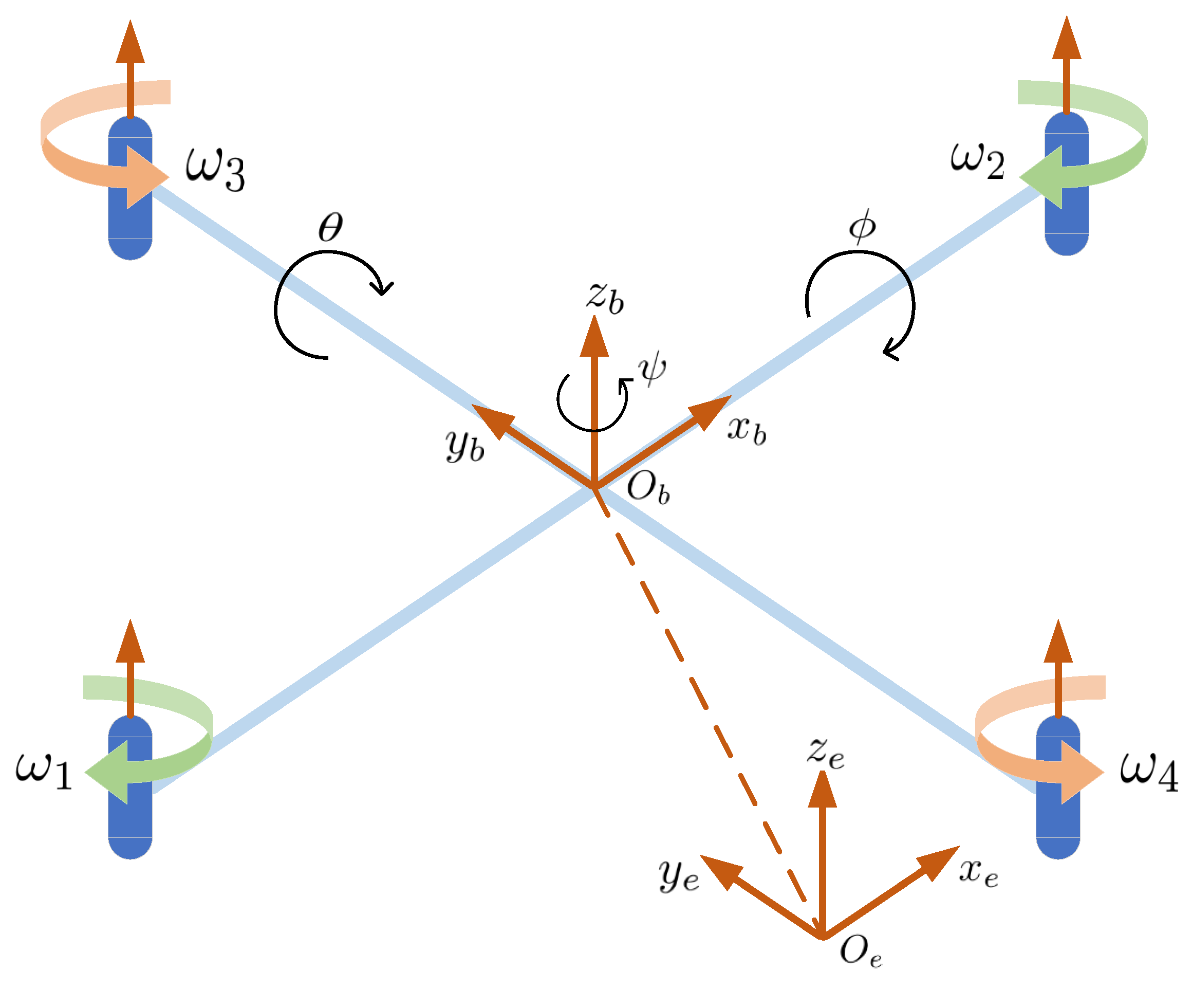
2. System Description

The design of a quadrotor UAV involves both position and attitude control. The structure of the quadrotor is illustrated in Figure 1. The origin $O_b$ is the center of the quadrotor UAV. The roll and pitch angles $(\varphi ,\theta )$ are coupled to the global position $(x,y)$. To move in the $x_e$ or $y_e$ direction, it is usually necessary to adjust the pitch or roll angle $(\theta ,\varphi )$, while the yaw angle $\left(\psi \right)$ changes the direction of the UAV’s travel. Additionally, let $\mathit{X}={\left[x,y,z\right]}^{\mathrm{T}}$ represent the center of position of the quadrotor.

The quadrotor UAV dynamics model is established as follows [13]:

$$m\ddot{\mathit{X}}+mg{\mathit{e}}_3=\mathit{R}\left(\mathsf{\Theta }\right)\mathit{U}$$

(1)

$$\mathit{J}\left(\mathsf{\Theta }\right)\ddot{\mathsf{\Theta }}+\mathit{C}\left(\mathsf{\Theta },\dot{\mathsf{\Theta }}\right)\dot{\mathsf{\Theta }}=\mathit{\tau }$$

(2)

with

$$\mathit{R}\left(\mathsf{\Theta }\right)=\left[\begin{array}{ccc}C\psi C\theta & C\psi S\theta S\varphi -S\psi C\varphi & C\psi S\theta C\varphi +S\psi S\varphi \\ S\psi C\theta & S\psi S\theta S\varphi +C\psi C\varphi & S\psi S\theta C\varphi -C\psi S\varphi \\ -S\theta & C\theta S\varphi & C\theta C\varphi \end{array}\right]$$

(3)

where ${\mathit{e}}_3={\left[0,0,1\right]}^{\mathrm{T}}$; m is the mass of the quadrotor UAV; g is the gravitational constant; $\mathit{U}={\left[0,0,f\right]}^{\mathrm{T}}$ is the total thrust vector; $\mathit{\tau }\in {\mathbb{R}}^3$ is the moment input by the attitude system. $S·$ is the sine function $sin(·)$ and $C·$ is the cosine function $cos(·)$. The positive definite diagonal matrix $\mathit{I}=\mathrm{diag}\left([I_{11},I_{22},I_{33}\right])$. The symmetry matrix $\mathit{J}\left(\mathsf{\Theta }\right)\in {\mathbb{R}}^{3\times 3}$ and matrix $\mathit{C}\left(\mathsf{\Theta },\dot{\mathsf{\Theta }}\right)\in {\mathbb{R}}^{3\times 3}$ are given by

$$\mathit{J}\left(\mathsf{\Theta }\right)=\left[\begin{array}{ccc}{I}_{11}& 0& -I_{11}S\theta \\ 0& I_{22}{C}^2\varphi +I_{33}{S}^2\varphi & \left(I_{22}-I_{33}\right)C\varphi S\varphi C\theta \\ -I_{11}S\theta & \left(I_{22}-I_{33}\right)C\varphi S\varphi C\theta & I_{11}{S}^2\theta +I_{22}{S}^2\varphi C^2\theta +I_{33}{C}^2\varphi C^2\theta \end{array}\right]$$

(4)

$$\mathit{C}\left(\mathsf{\Theta },\dot{\mathsf{\Theta }}\right)=\left[\begin{array}{ccc}{c}_{11}& c_{12}& c_{13}\\ c_{21}& c_{22}& c_{23}\\ c_{31}& c_{32}& c_{33}\end{array}\right]$$

(5)

with

$$\begin{array}{cc}\hfill c_{11}& =0,\hfill \\ \hfill c_{12}& =\left(I_{22}-I_{33}\right)\left(\dot{\theta }C\varphi S\varphi +\dot{\psi }{S}^2\varphi C\theta -\dot{\psi }{C}^2\varphi C\theta \right)-I_{11}\dot{\psi }C\theta ,\hfill \\ \hfill c_{13}& =\left(I_{22}-I_{33}\right)\dot{\psi }C\varphi S\varphi C^2\theta ,\hfill \\ \hfill c_{21}& =\left(I_{33}-I_{22}\right)\left(\dot{\theta }C\varphi S\varphi +\dot{\psi }{S}^2\varphi C\theta -\dot{\psi }{C}^2\varphi C\theta \right)+I_{11}\dot{\psi }C\theta ,\hfill \\ \hfill c_{22}& =\left(I_{33}-I_{22}\right)\varphi C\varphi S\varphi ,\hfill \\ \hfill c_{23}& =-I_{11}\dot{\psi }S\theta C\theta +I_{22}\dot{\psi }{S}^2\varphi C\theta S\theta +I_{33}\dot{\psi }{C}^2\varphi S\theta C\theta ,\hfill \\ \hfill c_{31}& =\left(I_{33}-I_{22}\right)\dot{\psi }C\varphi S\varphi S\theta -I_{11}\dot{\theta }C\theta ,\hfill \\ \hfill c_{32}& =\left(I_{33}-I_{22}\right)\left(\dot{\psi }C\varphi S\varphi S\theta -\dot{\varphi }{S}^2\varphi C\theta -\dot{\varphi }{C}^2\varphi C\theta \right)+I_{11}\dot{\psi }S\theta C\theta \hfill \\ \hfill & \phantom{=}-I_{22}\dot{\psi }{S}^2\varphi C\theta S\theta -I_{33}\dot{\psi }C\varphi S\theta C\theta ,\hfill \\ \hfill c_{33}& =\left(I_{33}-I_{22}\right)\varphi C\varphi S\varphi C^2\theta -I_{22}\dot{\theta }{S}^2\varphi C\theta S\theta -I_{33}\dot{\theta }{C}^2\varphi S\theta C\theta \hfill \\ \hfill & \phantom{=}+I_{11}\dot{\theta }S\theta C\theta .\hfill \end{array}$$

(6)

This paper addresses the trajectory tracking problem for UAVs using NMPC with the dynamic model of the UAV described above. To ensure the UAV’s control smoothness requirements, control increments are weighted in the cost function. Thus, $\Delta u=u_i-u_{i-1}\to 0$ ($i=1,2,3,\dots$) is reached when $t\to \infty$. The C/GMRES method is employed to reduce the computational burden of NMPC. The barrier methods are used to transform the original optimization problem into an unconstrained one. Additionally, the algorithm’s attraction domain intersects with a Lyapunov-based control method to ensure the system’s closed-loop stability. The system is divided into inner-loop and outer-loop control, as shown in Figure 2. The outer-loop position controller uses the improved C/GMRES method to efficiently solve the nonlinear optimization problem, allowing for real-time adjustment of the system’s position and ensuring accurate trajectory tracking. The inner-loop attitude controller uses a PID control strategy to quickly adjust the attitude and stabilize the system’s flight state.

3. Trajectory Tracking Controller Design

3.1. Brief Description of NMPC Controller

Assuming that the reference trajectory is appropriate and does not violate the physical limits of the UAV [30]. We consider both the UAV’s force constraints and the constraints on the rate of change simultaneously. The cost function is constructed based on the UAV’s position dynamics model as follows:

$$\begin{array}{cc}\hfill \underset{\widehat{u}\left(·\right)}{min}& {\int }_t^{t+T}{∥\widehat{\tilde{\mathit{x}}}\left(s\right)∥}_Q^2+{∥\widehat{\mathit{u}}\left(s\right)∥}_R^{2}ds+{∥\widehat{\tilde{\mathit{x}}}\left(t+T\right)∥}_P^2\hfill \\ \hfill \mathrm{s}.\mathrm{t}.& \dot{\widehat{\mathit{x}}}\left(s\right)=f\left(\widehat{\mathit{x}}\left(s\right),\widehat{\mathit{u}}\left(s\right)\right),s\in \left[t,t+T\right)\hfill \\ \hfill & \widehat{\mathit{x}}\left(t\right)=\mathit{x}\left(t\right),\widehat{\mathit{u}}\left(t\right)=\mathit{u}\left(t\right)\hfill \\ \hfill & {∥\widehat{\mathit{u}}\left(s\right)∥}_{\infty }⩽u_{max},s\in \left[t,t+T\right)\hfill \end{array}$$

(7)

where T is the prediction horizon; $\widehat{\mathit{x}}\left(\mathit{s}\right)$ represents the current state; ${\mathit{x}}_r\left(\mathit{s}\right)$ represents the reference state; $\widehat{\mathit{u}}\left(t\right)$ represents the control sequence; $\widehat{\tilde{\mathit{x}}}\left(s\right)=\widehat{\mathit{x}}\left(s\right)-{\mathit{x}}_r\left(s\right)$ represents the error in predicted tracking; ${\mathit{u}}_{max}$ and $\Delta {\mathit{u}}_{max}$ denote the maximum magnitudes of control input and control variations, respectively; $Q,R,S$ are positive definite weighting matrices. ${∥\widehat{\tilde{\mathit{x}}}\left(s\right)∥}_Q^2={\widehat{\tilde{\mathit{x}}}}^{\mathrm{T}}\left(s\right)Q\widehat{\tilde{\mathit{x}}}\left(s\right)$, ${∥\widehat{\mathit{u}}\left(s\right)∥}_R^2={\widehat{\mathit{u}}}^{\mathrm{T}}\left(s\right)R\widehat{\mathit{u}}\left(s\right)$ and ${∥\widehat{\tilde{\mathit{x}}}(t+T)∥}_P^2={\widehat{\tilde{\mathit{x}}}(t+T)}^{\mathrm{T}}P\widehat{\tilde{\mathit{x}}}(t+T)$.

The C/GMRES-based method is computed and implemented using a discrete-time formulation but remains based on continuous time t. Therefore, the discretization problem must be addressed at each continuous time t, ensuring the stability and accuracy of the discretization process. Assuming a prediction interval of N steps, the step size is $\delta =T/N$, which is referred to as the sampling period. The discretization of the above equation is as follows:

$$\begin{array}{cc}\hfill P_1\left(\mathit{x}\right):\underset{{\widehat{u}}_i}{min}& J=\sum _{i=0}^{N-1}\left({∥{\tilde{x}}_i∥}_Q^2+{∥{\widehat{u}}_i∥}_R^2\right)\delta +{∥{\tilde{x}}_N∥}_P^2\hfill \\ \hfill \mathrm{s}.\mathrm{t}.& \dot{\widehat{\mathit{x}}}\left(s\right)=f\left(\widehat{\mathit{x}}\left(s\right),\widehat{\mathit{u}}\left(s\right)\right),s\in \left[t,t+T\right)\hfill \\ \hfill & \widehat{\mathit{x}}\left(t\right)=\mathit{x}\left(t\right),\widehat{\mathit{u}}\left(t\right)=\mathit{u}\left(t\right)\hfill \\ \hfill & {∥\widehat{\mathit{u}}\left(s\right)∥}_{\infty }⩽u_{max},s\in \left[t,t+T\right)\hfill \end{array}$$

(8)

with the guarantee that the system is differentiable and the constraints hold, the Karush–Kuhn–Tucker (KKT) condition [31] provides a first-order necessary condition for the optimal solution ${\mathit{U}}^{*}$ of the optimization problem $P_1\left(\mathit{x}\right)$. Sequential quadratic programming and the interior point method can be used to solve the KKT condition for $P_1\left(\mathit{x}\right)$. However, these methods rely on continuous linearization. To address this, the C/GMRES numerical algorithm will be used to speed up the numerical computation of NMPC, considering both the onboard computational burden and computational efficiency. The standard C/GMRES can only solve optimization problems with equality constraints. Then, we relax this restriction and propose an improved strategy to compute the optimal solution under the inequality constraints, which leads to a smoother and globally stabilized control process.

3.2. Improved Efficient NMPC

This section introduces a smoothing constraint on the control increment and a contraction constraint to improve the smoothness of the control process and ensure global convergence. Finally, an efficient NMPC algorithm is proposed to ensure that the solution obtained during the optimization process satisfies the conditions and constraints.

3.2.1. Smoothness Constraint Term for Control Increments

The rate of change of the control input must be considered in the actual control process. Otherwise, excessive changes in the control strategy can lead to violent system oscillations. In addition, the optimization algorithm might produce significant control input variations between successive steps, which could result in an unstable system response.

Firstly, the control sequence is defined as ${\left\{{\widehat{\mathit{u}}}_i^{*}\right\}}_{i=0}^N$, where ${\mathit{u}}_i$ is the ith control input component at the current time step, and ${\mathit{u}}_{i-1}$ is the corresponding control input component at the previous time step. The sum of squares of control increments is introduced to address potential numerical instability in the search for an optimal solution to an optimization problem. When the control inputs change significantly between time steps, the penalty function penalizes these changes. This function finds a solution that satisfies the constraints during the optimization process. As a result, the final solution meets the requirements. The constraint with the penalty term is then defined as follows:

$$\mathit{\vartheta }\left({\widehat{\mathit{u}}}_i\right)=\rho ·\sum _{i=1}^N{\left(\Delta {\widehat{\mathit{u}}}_i\right)}^2$$

(9)

where $\Delta {\widehat{\mathit{u}}}_i={\widehat{\mathit{u}}}_i^{*}-{\widehat{\mathit{u}}}_{i-1}^{*}$, and the penalty factor $\rho$ is introduced to emphasize the impact of $\mathit{\vartheta }\left({\widehat{\mathit{u}}}_i\right)$. A larger value of $\rho$ causes $\mathit{\vartheta }\left({\widehat{\mathit{u}}}_i\right)$ to $\Delta {\widehat{\mathit{u}}}_i$ more significantly, while a smaller $\rho$ reduces this penalty. The parameter $\rho$ is introduced to balance the attainment of an optimal solution with the satisfaction of constraints, thereby preventing the imposition of excessively stringent conditions. To facilitate the optimization process, it is typically necessary to fine-tune the value of $\rho$, ensuring a more effective and efficient solution. The modified optimal control problem (OCP) $\left(P_2\left(\mathit{x}\right)\right)$, with the penalty term incorporated into the cost function, can be formulated as follows:

$$\begin{array}{cc}\hfill P_2\left(\mathit{x}\right):\underset{{\widehat{u}}_i}{min}& J=\sum _{i=0}^{N-1}\left({∥{\widehat{\tilde{\mathit{x}}}}_i∥}_Q^2+{∥{\widehat{\mathit{u}}}_i∥}_R^2+\epsilon ·\mathit{\vartheta }\left({\widehat{\mathit{u}}}_i\right)\right)\delta +{∥{\widehat{\tilde{\mathit{x}}}}_N∥}_P^2\hfill \\ \hfill \mathrm{s}.\mathrm{t}.& {\widehat{\mathit{x}}}_{i+1}=f\left({\widehat{\mathit{x}}}_i,{\widehat{\mathit{u}}}_i\right)+{\widehat{\mathit{x}}}_i\hfill \\ \hfill & {\widehat{\mathit{x}}}_0=\mathit{x}\left(t\right)\hfill \\ \hfill & {∥\widehat{\mathit{u}}\left(s\right)∥}_{\infty }⩽{\mathit{u}}_{max},s\in \left[t,t+T\right)\hfill \end{array}$$

(10)

where $\mathit{\vartheta }\left({\widehat{\mathit{u}}}_i\right)$ represents a soft constraint on the control input $\Delta {\widehat{\mathit{u}}}_i$. It can moderately violate the constraints in the optimization process, making it more flexible. Especially when the constraints are difficult to handle, a feasible solution can be obtained by appropriately adjusting the strength of the penalty term, thus adapting to the different needs of the problem. The impact of different parameter values $\epsilon$ in (10) on numerical convergence should be discussed. Utilizing the C/GMRES method for approximate computation of solutions in $P_2\left(\mathit{x}\right)$, the following assumptions and lemmas are made within the context of practical applications:

Assumption 1 

([32]). For each $\epsilon ={\epsilon }_d>0$, there exists a bounded solution ${\mathit{U}}_n$.

The C/GMRES method is based on the conditions required for solving Pontryagin’s Maximum Principle (PMP) to attain the optimal solution for $P_2\left(\mathit{x}\right)$, rather than the KKT conditions. Therefore, the sufficiency of PMP for addressing the KKT conditions is explored first.

Lemma 1 

([28]). A point satisfies the PMP condition of $P_2\left(\mathit{x}\right)$, sufficiently solving its KKT conditions.

Proof. 

The proof of Lemma 1 is presented in Appendix A.1. □

Lemma 2. 

Assume Assumption 1 holds, and $0<{\epsilon }_{n+1}<{\epsilon }_n$ is a solution to $P_2\left(\mathit{x}\right)$ with optimal solutions ${\overline{\mathit{U}}}_{n+1}$ and ${\overline{\mathit{U}}}_n$. Then, the following inequalities can hold as follows:

$$\overline{\mathit{J}}\left({\overline{\mathit{U}}}_{n+1},{\epsilon }_{n+1}\right)\le \overline{\mathit{J}}\left({\overline{\mathit{U}}}_n,{\epsilon }_n\right)$$

$$\overline{\mathit{J}}\left({\overline{\mathit{U}}}_{n+1}\right)\ge \overline{\mathit{J}}\left({\overline{\mathit{U}}}_n\right),\vartheta \left({\overline{\mathit{U}}}_n\right)\ge \vartheta \left({\overline{\mathit{U}}}_{n+1}\right)$$

Proof. 

The proof of Lemma 2 is presented in Appendix A.2. □

Lemma 3 

([29]). ${\left\{{\epsilon }_{\mathrm{n}}\right\}}_{n=1}^N$ is a decreasing sequence satisfying $0<{\epsilon }_{n+1}<{\epsilon }_n$, and when $n\to +\infty$, there exists ${\epsilon }_n$ sufficiently small. Based on Assumption 1, ${\mathit{U}}_n$ converges to ${\mathit{U}}^{*}$.

Lemma 4 

([29]). Consider Lemmas 1 and 3. $P_2\left(\mathit{x}\right)$ is the optimal solution. Then, the above approximately solves $P_1\left(\mathit{x}\right)$ with a sufficiently little ε in $P_2\left(\mathit{x}\right)$.

3.2.2. C/GMRES Algorithm

For $P_2\left(\mathit{x}\right)$, the Hamiltonian function is defined as follows:

$$\mathit{H}\left(\mathit{x},\mathit{u},\mathit{\kappa }\right)={∥\mathit{x}-{\mathit{x}}_r∥}_Q^2+{∥\mathit{u}∥}_R^2+\mathit{\vartheta }\left(\mathit{u},{\mathit{u}}_{max}\right)+{\mathit{\kappa }}^{\mathrm{T}}f\left(\mathit{x},\mathit{u}\right)$$

where $\mathit{\kappa }$ represents the costate [28], and ${\left\{{\widehat{\mathit{u}}}_i^{*}\right\}}_{i=0}^{N-1}$ is the global optimal solution to $P_2\left(\mathit{x}\right)$. The costate sequence ${\left\{{\mathit{\kappa }}_i\right\}}_{i=1}^N$ satisfies ${\widehat{\mathit{x}}}_{i+1}=f\left({\widehat{\mathit{x}}}_i,{\widehat{\mathit{u}}}_i\right)+{\widehat{\mathit{x}}}_i$ and ${\widehat{\mathit{x}}}_0=\mathit{x}\left(t\right)$, and the following conditions:

$${\widehat{\mathit{x}}}_{i+1}={\mathit{x}}_i+f\left({\mathit{x}}_i,{\mathit{u}}_i\right)\delta$$

(11)

$${\mathit{\kappa }}_N={\displaystyle \frac{\partial {∥{\tilde{\mathit{x}}}_N∥}_P^2}{\partial \mathit{x}}}$$

(12)

$${\mathit{\kappa }}_i={\mathit{\kappa }}_{i+1}+{\mathit{H}}_x\left({\widehat{\mathit{x}}}_i,{\widehat{\mathit{u}}}_i^{*},{\mathit{\kappa }}_{i+1},\epsilon \right)\delta$$

(13)

$${\mathit{H}}_u\left({\widehat{\mathit{x}}}_i,{\widehat{\mathit{u}}}_i^{*},{\mathit{\kappa }}_{i+1},\epsilon \right)=0$$

(14)

Equations (11) and (13) represent recursive relationships, while ${\widehat{\mathit{x}}}_0=\mathit{x}\left(t\right)$ and (12) serve as boundary conditions. ${\mathit{H}}_x$ and ${\mathit{H}}_u$ are the partial derivatives of the Jacobian matrix $\mathit{H}$ with respect to $\mathit{x}$ and $\mathit{u}$, respectively. The sequence ${\left\{{\widehat{\mathit{u}}}_i^{*}\right\}}_{i=1}^{N-1}$ is determined by (14). Starting from ${\widehat{\mathit{x}}}_0=\mathit{x}\left(t\right)$ and iterating through (11), Equations (12) and (13) are processed in reverse order of time. The state sequence ${\left\{{\widehat{\mathit{x}}}_i\right\}}_{i=0}^{N-1}$ and the costate sequence ${\left\{{\mathit{\kappa }}_i\right\}}_{i=1}^N$ are explicit functions of ${\dot{\mathit{U}}}^{*}$. We then substitute these into (14) to construct the system of equations:

$$\mathit{F}\left({\dot{\mathit{U}}}^{*},\mathit{x},\mathit{\epsilon }\right)=\left[\begin{array}{c}{\mathit{H}}_u\left({\widehat{\mathit{x}}}_0,{{\widehat{\mathit{u}}}^{*}}_0,{\mathit{\kappa }}_1,\epsilon \right)\\ {\mathit{H}}_u\left({\widehat{\mathit{x}}}_1,{{\widehat{\mathit{u}}}^{*}}_1,{\kappa }_2,\epsilon \right)\\ {\mathit{H}}_u\left({\widehat{\mathit{x}}}_2,{{\widehat{\mathit{u}}}^{*}}_2,{\kappa }_3,\epsilon \right)\\ ⋮\\ {\mathit{H}}_u\left({\widehat{\mathit{x}}}_{N-1},{{\widehat{\mathit{u}}}^{*}}_{N-1},{\kappa }_N,\epsilon \right)\end{array}\right]$$

(15)

To solve (15) at time t, standard approaches involve computing the Jacobian matrix, Hessian matrix, and their inverses using iterative methods. However, this process is computationally expensive and time-consuming. Instead, numerical continuum methods and forward difference generalized minimum residuals (FDGMRES) avoid the need to compute matrix inverses. The FDGMRES method, which combines forward difference approximation combined with GMRES, is described as follows:

$$\dot{\widehat{\mathit{U}}}=\mathrm{FDGMRES}\left(\widehat{\mathit{U}},\mathit{x},\dot{\mathit{x}},\tilde{\dot{\widehat{\mathit{U}}}},{\mathit{k}}_{max},\epsilon \right)$$

(16)

where $\dot{\mathit{x}}$ is approximated as $\dot{\mathit{x}}\left(t\right)=\left(\mathit{x}\left(t+\delta \right)-\mathit{x}\left(t\right)\right)/\delta$; $k_{max}$ represents the maximum number of iterations; $\tilde{\dot{\widehat{\mathit{U}}}}$ is the initial feasible value; $\widehat{\mathit{U}}$ is a feasible initial control input sequence [27]. $\left(P_2\left(\mathit{x}\right)\right)$ can be solved efficiently by applying C/GMRES. Algorithm 1 summarizes the FDGMRES algorithm for solving ${\dot{\mathit{U}}}^{*}$:

Algorithm 1: FDGMRES algorithm for ${\dot{\mathit{U}}}^{*}$

1. Initialize $t=0$, $l=0$, ${\mathit{x}}_0=\mathit{x}\left(0\right)$, $n=n+1$;

2. Get $\tilde{\dot{\widehat{\mathit{U}}}}$ by $∥\mathit{F}\left({\widehat{\mathit{U}}}_0,\mathit{x}\left(t_0\right),0\right)∥=0$;

3. Get $\mathit{F}$ from (14) and partial derivative ${\mathit{F}}_d$;

4. $\mathit{b}=\mathit{A}\ast \mathit{F}-(1/h)\ast \mathit{F}$, $\widehat{\mathit{r}}=\mathit{b}-{\mathit{F}}_d\left({\mathit{U}}^{*},\mathit{x}+h\dot{\mathit{x}},\tilde{\dot{\widehat{\mathit{U}}}},\mathrm{zeros}(nX,1)\right)$, $\mathit{v}1=\widehat{\mathit{r}}/\parallel \widehat{\mathit{r}}\parallel$;

5. while $k<k_{max}$ do

6.     get ${\mathit{x}}_{k+1}=\mathit{x}\left(t+\delta \right)$ and ${\dot{\mathit{x}}}_k=({\mathit{x}}_{k+1}-{\mathit{x}}_k)/\delta$;

7.     ${\mathit{v}}_{k+1}={\mathit{F}}_d\left({\mathit{U}}^{*},\mathit{x}+h\dot{\mathit{x}},{\mathit{v}}_k(nU,N),\mathrm{zeros}(nX,1)\right)$;

8.     For $j=1:1:k$

9.        ${\mathit{h}}_{j,k}={{\mathit{v}}_k}^{\mathrm{T}}\ast {\mathit{v}}_k$;

10.       ${\mathit{v}}_{k+1}={\mathit{v}}_{k+1}-{\mathit{h}}_{j,k}\ast {\mathit{v}}_k$;

11.    End for

12.    ${\mathit{h}}_{k+1,k}=\parallel {\mathit{v}}_{k+1}\parallel$; ${\mathit{v}}_{k+1}={\mathit{v}}_{k+1}/\parallel {\mathit{v}}_{k+1}\parallel$; $\mathit{e}=[1,\mathrm{zeros}(k,1\left)\right]$;

13.    ${\widehat{\mathit{h}}}_k={\mathit{h}}_k(1:k+1,1:k)$; ${\mathit{m}}_k={\left({\widehat{\mathit{h}}}_k\right)}^{-1}\ast \parallel \widehat{\mathit{r}}\parallel \ast \mathit{e}$; $\rho =\parallel \parallel \widehat{\mathit{r}}\parallel \ast \mathit{e}-{\widehat{\mathit{h}}}_k\ast {\mathit{m}}_k\parallel$;

14.    If $\rho <\mathrm{tol}$

15.       break;

16.    End if

17. End While

18. ${\dot{\mathit{U}}}^{*}={\dot{\widehat{\mathit{U}}}}^{*}+{\mathit{v}}_k\ast {\mathit{m}}_k$;

19. $t=t+\delta$, $k=k+1$.

3.2.3. Adding Stability Constraints

Nonetheless, while it is possible to achieve the global optimal solution, the closed-loop stability of the system cannot be assured due to the limited prediction horizon. Therefore, the following solution is needed. Suppose there is a feedback control rule $\mathit{u}\left(t\right)=\mathit{\zeta }\left(\mathit{x}\right(t\left)\right)$, which in some stable region ensures that the control input $\mathit{u}$ satisfies a particular constraint and makes the system asymptotically stable at the origin. According to the inverse Lyapunov theorem [33], this means that we can find some specific type of function ${\gamma }_i(·)(i=1,2,3,4)$ and a continuously differentiable Lyapunov function $V\left(\mathit{x}\right)$ such that the system satisfies certain inequalities, thus proving its stability. ${\gamma }_1∥\mathit{x}∥\le V\left(\mathit{x}\right)\le {\gamma }_2∥\mathit{x}∥$, ${\displaystyle \frac{\partial V}{\partial \mathit{x}}}f(\mathit{x},\mathit{\zeta }\left(\mathit{x}\right))\le -{\gamma }_3∥\mathit{x}∥$, $∥{\displaystyle \frac{\partial V\left(\mathit{x}\right)}{\partial \mathit{x}}}∥\le {\gamma }_4∥\mathit{x}∥$. For all $\mathit{x}\in O\in R^n$, where O is an open neighborhood of the origin, we denote the region ${\Omega }_O\in O$ as the stability region of the closed-loop system under control $\mathit{u}=\mathit{\zeta }\left(\mathit{x}\right)$ [34].

Since the system uses only the first column of the control sequence ${\mathit{U}}^{*}$ obtained from the prediction sequence $[t,t+\delta ]$, only the first prediction interval is considered.

$$\begin{array}{cc}\hfill P_3\left(\mathit{x}\right):\underset{{\widehat{u}}_i}{min}& J=\sum _{i=0}^{N-1}\left({∥{\widehat{\tilde{\mathit{x}}}}_i∥}_Q^2+{∥{\widehat{\mathit{u}}}_i∥}_R^2+\epsilon ·\mathit{\vartheta }\left({\widehat{\mathit{u}}}_i\right)\right)\delta +{∥{\widehat{\tilde{\mathit{x}}}}_N∥}_P^2\hfill \\ \hfill \mathrm{s}.\mathrm{t}.& {\widehat{\mathit{x}}}_{i+1}=f\left({\widehat{\mathit{x}}}_i,{\widehat{\mathit{u}}}_i\right)+{\widehat{\mathit{x}}}_i\hfill \\ \hfill & {\widehat{\mathit{x}}}_0=\mathit{x}\left(t\right)\hfill \\ \hfill & {∥\widehat{\mathit{u}}\left(s\right)∥}_{\infty }⩽{\mathit{u}}_{max},s\in \left[t,t+T\right)\hfill \\ \hfill & {\displaystyle \frac{\partial V}{\partial \mathit{x}}}f\left(\mathit{x}\left(t\right),\mathit{u}\left(t\right)\right)\le {\displaystyle \frac{\partial V}{\partial \mathit{x}}}f\left(\widehat{\mathit{x}}\left(t\right),\mathit{\zeta }\left(\widehat{\mathit{x}}\left(t\right)\right)\right)\hfill \end{array}$$

(17)

where $V\left(·\right)$ is the Lyapunov function and designed in Section 3.2.4; $\mathit{\zeta }\left(·\right)$ is the auxiliary control law based on the Lyapunov function. When $t\in [t,t+\delta )$, the optimal solution of the optimization problem is $U^{*}$. The constraints ${\displaystyle \frac{\partial V}{\partial \mathit{x}}}f\left(\mathit{x}\left(t\right),\mathit{u}\left(t\right)\right)\le {\displaystyle \frac{\partial V}{\partial \mathit{x}}}f\left(\widehat{\mathit{x}}\left(t\right),\mathit{\zeta }\left(\widehat{\mathit{x}}\left(t\right)\right)\right)$ ensure that the time derivative $V\left(\mathit{x}\right)$ of the Lyapunov function at time t is less than or equal to the value of the nonlinear control law $u=\zeta \left(x\right)$. This holds when the control law is applied in a sample-and-hold fashion within a closed-loop system. Using the state measurements obtained at each synchronized sampling time, it can be demonstrated that the control law designed in this paper inherits the stability and robustness of the Lyapunov-based control law $\zeta \left(x\right)$. This is true provided that system data loss is not considered [35]. One of the main properties of stability constraints is that they have the same stability domain as the nonlinear control law $\zeta \left(x\right)$. That means the system is stable when the sampling time and the upper limit of perturbation are small enough [36,37]. In $P_3\left(\mathit{x}\right)$, without compromising the stability of the tracking control, a component that adaptively adjusts the prediction horizon is added to $P_2\left(\mathit{x}\right)$, which reduces the inconvenience caused by adjusting the parameters. Meanwhile, the adaptive adjustment of the prediction horizon can reduce the optimization scale of the NMPC.

3.2.4. Lyapunov-Based Auxiliary Control Law Design

The Lyapunov-based control method is widely used in nonlinear UAV systems, as it can demonstrate the global stability of the entire system [36]. Therefore, the fixed-time integral sliding mode control method can be adopted to construct $\mathit{\zeta }\left(\mathit{x}\right)$. According to [38,39], for system $\dot{\mathit{x}}\left(t\right)=f\left(\mathit{x},\mathit{u}\right)$, if there exists a Lyapunov function on its domain that satisfies $\dot{V}\left(\mathit{x}\right)\le -aV{\left(\mathit{x}\right)}^{\alpha }-bV{\left(\mathit{x}\right)}^{\beta }$. Here, $a,b>0$ and $0<\beta <1<\alpha$. Furthermore, the system is globally fixed-time stable, and the stability time is $T\le {\displaystyle \frac{1}{a(\alpha -1)}}+{\displaystyle \frac{1}{b(\beta -1)}}$.

The position loop system can be written as ${\dot{\mathit{X}}}_1={\mathit{X}}_2={\displaystyle \frac{\mathit{U}}{m}}-g{\mathit{e}}_3$, where ${\mathit{X}}_2={[\dot{x},\dot{y},\dot{z}]}^{\mathrm{T}}$. Then, design a virtual controller [40]: ${\mathit{u}}_{nom}=-k_1{\mathrm{sig}}^{p_1}\left({\mathit{X}}_1\right)-k_1{\mathrm{sig}}^{q_1}\left({\mathit{X}}_1\right)-k_2{\mathrm{sig}}^{p_2}\left({\mathit{X}}_2\right)-k_2{\mathrm{sig}}^{q_2}\left({\mathit{X}}_2\right)$. Choose $k_1$, $k_2$ to ensure that the second-order polynomial ${\lambda }^2+k_2\lambda +k_1$ is Hurwitz. And $0<p_1<1,q_1=2p_1/(1+p_1),p_2>1,q_2=2p_2/(1+p_2)$.

For the error system ${\dot{\mathit{X}}}_2-{\ddot{\mathit{X}}}_{2r}={\dot{\mathit{X}}}_{2e}={\displaystyle \frac{\zeta }{m}}-g{\mathit{e}}_3-{\ddot{\mathit{X}}}_{2r}$, where ${\mathit{X}}_{2r}={[x_d,y_d,z_d]}^{\mathrm{T}}$ and ${\ddot{\mathit{X}}}_{2r}={[{\ddot{x}}_d,{\ddot{y}}_d,{\ddot{z}}_d]}^{\mathrm{T}}$. Its Lyapunov candidate function satisfies ${\lambda }_1{∥{\mathit{x}}_e∥}^2\le V\left(\mathit{x}\right)\le {\lambda }_2{∥{\mathit{x}}_e∥}^2$, where ${\lambda }_1,{\lambda }_2\in R$. Select the sliding surface as follows:

$$\mathit{s}={\mathit{X}}_{2e}-{\mathit{X}}_{2r}\left(0\right)+{\int }_0^t\left(-{\displaystyle \frac{{\mathit{u}}_{nom}}{m}}+g{\mathit{e}}_3\right)dt$$

(18)

then, taking its derivative yields

$$\dot{\mathit{s}}={\dot{\mathit{X}}}_{2e}-{\displaystyle \frac{{\mathit{u}}_{nom}}{m}}+g{\mathit{e}}_3={\displaystyle \frac{\mathit{\zeta }}{m}}+{\displaystyle \frac{{\mathit{u}}_{nom}}{m}}$$

(19)

Theorem 1. 

Considering the dynamic error system ${\dot{\mathit{X}}}_{2e}={\displaystyle \frac{\zeta }{m}}-g{\mathit{e}}_3-{\ddot{\mathit{X}}}_{2r}$, and selecting surface (18) as the sliding surface, the controller can be designed as follows:

$$\mathit{\zeta }=-{\gamma }_1{\mathrm{sig}}^{{\displaystyle \frac{b}{c}}}\left(\mathit{s}\right)-{\gamma }_2{\mathrm{sig}}^{{\displaystyle \frac{n}{m}}}\left(\mathit{s}\right)+{\mathit{u}}_{nom}$$

(20)

where ${\gamma }_1,{\gamma }_2$ is a positive number and $b<c,n>m$ are all positive odd integers, then there exists a fixed time T such that the system converges for $t>T$.

Proof. 

The proof of Theorem 1 is presented in Appendix A.3. □

Remark 1. 

According to ${\displaystyle \frac{\partial V}{\partial \mathit{x}}}f\left(\mathit{x}\left(t\right),\mathit{u}\left(t\right)\right)\le {\displaystyle \frac{\partial V}{\partial \mathit{x}}}f\left(\widehat{\mathit{x}}\left(t\right),\mathit{\zeta }\left(\widehat{\mathit{x}}\left(t\right)\right)\right)$, after obtaining the virtual control law based on Lyapunov, the intersection of the stability domains of the control law obtained from $P_2\left(\mathit{x}\right)$ can be obtained. The final solution obtained at last is also the solution obtained from $P_3\left(\mathit{x}\right)$. The improved NMPC controller in this paper can inherit the stability and robustness of $\mathit{\zeta }\left(\mathit{x}\right)$ [34].

Remark 2. 

Firstly, we use the control force $\mathit{U}$ and the desired ${\psi }_d$ obtained from the previous step to calculate the expected values ${\varphi }_d$ and ${\theta }_d$ for the angle. Secondly, we establish the desired values for the required roll and pitch angles, where ${\varphi }_d=arcsin\left({\displaystyle \frac{U_{a1}S{\psi }_d-U_{a2}C{\psi }_d}{∥{\mathit{U}}_a∥}}\right)$ and ${\theta }_d=arctan\left({\displaystyle \frac{U_{a1}C{\psi }_d+U_{a2}S{\psi }_d}{U_{a3}}}\right)$. In the case of ${\mathit{U}}_a={\left[U_{a1},U_{a2},U_{a3}\right]}^{\mathrm{T}}={\displaystyle \frac{1}{m}}\mathit{U}$, the obtained expected values of the attitude angles serve as inputs to the attitude controller. Therefore, the attitude controller is designed as ${\mathit{\tau }}_i=K_P^i{\mathit{e}}_i+K_I^i{\int }_0^t{\mathit{e}}_{i}dt+K_D^i{\displaystyle \frac{d{\mathit{e}}_i}{dt}}$, where $i\in \{\varphi ,\theta ,\psi \}$, ${\mathit{e}}_i$ represents the desired value of the angle minus the current value.

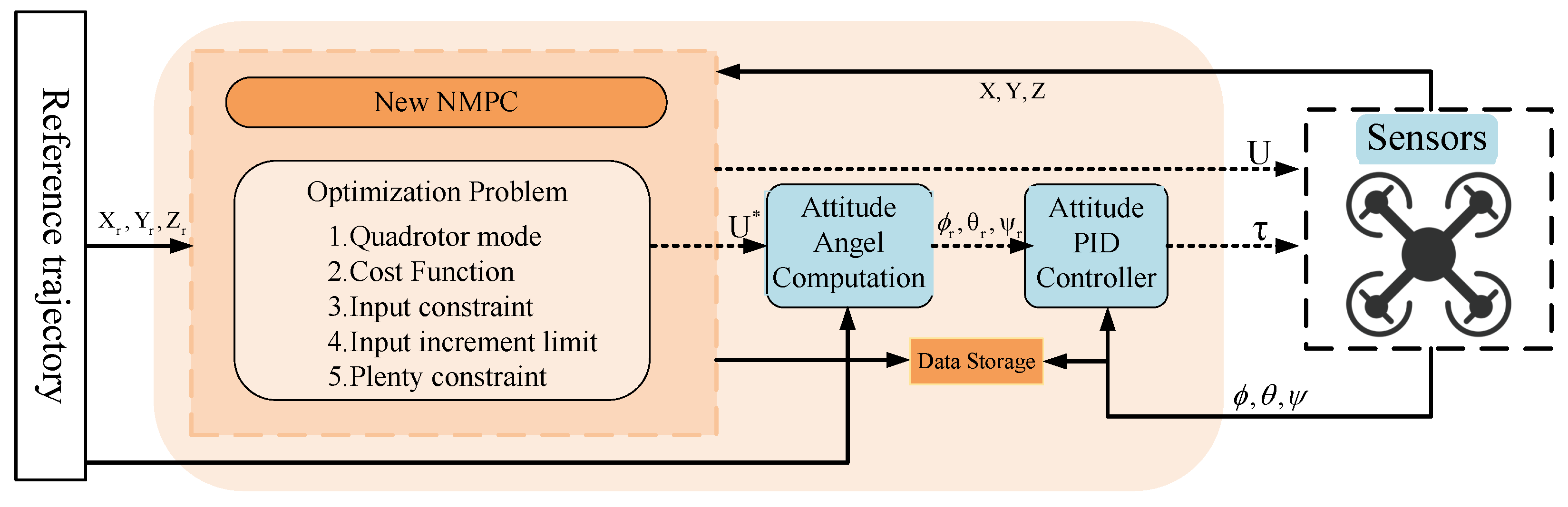
3.3. Algorithm Structure

In summary, the controller for the position loop increases the system’s rapidity without compromising the stability of the system’s tracking control. Then, the desired three angle values are obtained by attitude decoupling, and the design of the PID controller for the attitude loop is carried out. The control framework can be seen as follows: Firstly, the desired trajectory ($X,Y,Z$) is predefined and the fundamental cost function of the NMPC is formulated based on the established error model. This cost function comprises the error term, control term, and terminal error. A weighted sum of control increments is incorporated into the cost function to enhance control smoothness. Subsequently, the NMPC problem is solved using the C/GMRES method. A stability constraint is introduced to ensure that the stability region of the entire system is confined within the stability domain derived from Lyapunov’s method. Finally, the resulting control forces are decoupled to determine the desired angles for the PID control. This iterative process is repeated until the trajectory tracking is completed. Algorithm 2 covers the entire process:

Algorithm 2: Efficient-NMPC algorithm for UAV trajectory

1. Initialize $k_{max}=0$, $t_{prev}=0$, ${\mathit{x}}_0=\mathit{x}\left(0\right)$, ${\mathit{U}}_0=\mathit{u}\left(0\right)$, $N_{min}$, $N_{max}$, $\Delta N$;

2. While $k<k_{max}$ do

3. $k=k+1$; find $\tilde{\dot{\widehat{\mathit{U}}}}$ by $∥\mathit{F}\left({\widehat{\mathit{U}}}_0,\mathit{x}\left(t_0\right),0\right)∥=0$;

4. End while;

5. While $t<t_{end}$ do

6.     ${\mathit{x}}_{k+1}=\mathit{x}\left(t+\delta \right)$ and $\Delta {\mathit{x}}_k={\mathit{x}}_{k+1}-{\mathit{x}}_k$;

7.     ${\dot{\mathit{U}}}^{*}=\mathrm{FDGMRES}\left(\widehat{\mathit{U}},\mathit{x},\mathit{x}/\delta ,t,\tilde{\dot{\widehat{\mathit{U}}}},k_{max},\rho ,\epsilon \right)$;

8.     ${\mathit{U}}^{*}=\widehat{\mathit{U}}+{\dot{\mathit{U}}}^{*}\ast \delta ;$

9.     If ${\displaystyle \frac{\partial V}{\partial \mathit{x}}}f\left(\mathit{x}\left(t\right),\mathit{u}\left(t\right)\right)\le {\displaystyle \frac{\partial V}{\partial \mathit{x}}}f\left(\widehat{\mathit{x}}\left(t\right),\mathit{\zeta }\left(\widehat{\mathit{x}}\left(t\right)\right)\right)$

10.       $\mathit{U}={\mathit{U}}^{*}$; Else $\mathit{U}=\mathit{\zeta }$;

11.    End If

12.    Decoupling angel ${\varphi }_d=arcsin\left({\displaystyle \frac{U_{a1}S{\psi }_d-U_{a2}C{\psi }_d}{∥{\mathit{U}}_a∥}}\right)$, ${\theta }_d=arctan\left({\displaystyle \frac{U_{a1}C{\psi }_d+U_{a2}S{\psi }_d}{U_{a3}}}\right)$;

13.    Attitude controller ${\mathit{\tau }}_i=K_P^i{\mathit{e}}_i+K_I^i{\int }_0^t{\mathit{e}}_{i}dt+K_D^i{\displaystyle \frac{d{\mathit{e}}_i}{dt}}$;

14. End While

4. Simulation

4.1. Parameter Selection

In the simulation process, the mass of the quadrotor is 1.12 $\mathrm{kg}$. Inertia moments are $I_{11}=0.01 \mathrm{kg}·{\mathrm{m}}^2$, $I_{22}=0.0082 \mathrm{kg}·{\mathrm{m}}^2$, $I_{33}=0.0148 \mathrm{kg}·{\mathrm{m}}^2$. The initial position is set as ${\mathit{X}}_0=[0.1; 0.01; 0.01]$. The system’s sampling period is $t=0.1$ s. The desired trajectory is set as ${\mathit{X}}_d=[0.5sin\left(0.3t\right);0.3sin\left(0.6t\right);0.4]$. These trajectories are typical tracking control test trajectories with different reference tangential velocities and angular velocities, which pose a challenge to the tracking task. We can choose the following main parameters for the fixed-time integral sliding mode controller ${\gamma }_1=0.02$, ${\gamma }_2=0.02$, $b=3,c=2,n=4,m=3$. Since the initial solution of the FDGMRES function at the previous sampling time is often reasonable, the system can converge when the maximum number of iterations $k_{max}$ is reached. The weighting matrices $\mathit{R}=\mathrm{diag}\left(\right[1,1,1\left]\right)$, $\mathit{Q}=\mathrm{diag}\left(\right[100,100,320,300,340,160\left]\right)$ and $\mathit{P}=\mathrm{diag}\left(\right[110,130,100,300,80,40\left]\right)$. The coefficient is $\omega =0.4$, and the prediction increment is $\Delta N=5$.

4.2. Total Trajectory Simulation

When the sampling time $t=0.1$ s, the system tracking results are plotted in Figure 3. The blue trajectory represents the improved NMPC algorithm proposed in this paper and the red trajectory represents the algorithm used in reference [28]. The black trajectory represents the desired trajectory. Observing the trajectories at $t=0.6$ s, it can be seen that our proposed improved algorithm exhibits a significant improvement in rapidity, tracking the desired trajectory in a shorter time, with better performance and higher accuracy under the same conditions.

4.3. Improved NMPC Tracking Trajectory Performance and Efficiency Comparison

The NMPC algorithm utilizing the Hamiltonian solution method is employed to solve the position trajectory, with a sampling time of $t=0.2$ s. The grey trajectory curves for $N=5$ and light blue trajectory curves for $N=10$ are plotted. For a sampling time of $t=0.1$ s and $N=5$, the yellow trajectory curve with $d_{max}=1$ and the brown trajectory curve with $d_{max}=10$ are solved using the mC/GMRES method [28]. Additionally, with the same sampling time of $t=0.1$ s, the improved NMPC solution proposed in this paper is computed for various values of N and $d_{max}$. In

Table 1. The time required for each iteration of different algorithms.

Numerical Algorithm	Prediction Horizon	Average Time (s)
Improved NMPC	N = 5	0.0012
	N = 10	0.0041
	N = 15	0.0065
Hamiltonian-based NMPC	N = 5	0.15
	N = 10	0.19
	N = 15	1.28

, it can be seen that the average running time of the algorithms increases as N increases. However, when comparing the two algorithms with the same N, it can be seen that the average solution speed of the improved NMPC proposed in this paper is higher than that of the Hamiltonian-based NMPC. As shown in Figure 4 and Figure 5, the improved NMPC exhibits faster responsiveness and tracking with faster stabilization. As N and $d_{max}$ increase, the $e_x$ error rapidly converges close to 0. In Figure 4, the C/GMRES method does not achieve a steady-state trend as quickly as the improved NMPC, which can also be observed in $e_y$. It is observed that with the same $d_{max}$, the system response is faster when $N=10$; however, when both N and $d_{max}$ are lower, the tracking effect is not so good. In Figure 5, larger N and $d_{max}$ can make the system error smaller and the system response faster. So when N and $d_{max}$ exist relatively correctly, the system performance improves more obviously. The response time is shorter and the system error is smaller. It can be synthesized that the proposed improved NMPC demonstrates better overall performance within the tracking system, but comparisons reveal that different values of N and $d_{max}$ still result in slight variations in tracking effectiveness.

4.4. Performance under Wind Disturbance

When the system faces irregular and sudden wind disturbances during flight, its ability to recover quickly and accurately is essential for stability. To evaluate this recovery capability, wind disturbances of $ds=[2;-0.1;1]$ m/s lasting for $0.2$ s are applied at 10 s, 15 s, and 20 s, respectively. As shown in Figure 6, the mC/GMRES method demonstrates poor recovery performance in response to wind disturbances, while the improved NMPC proposed in this paper recovers more rapidly.

When subjected to smaller wind disturbances of $ds=[0.2;-0.1;0.3]$ m/s, lasting $0.2$ s at 10 s, 15 s, and 20 s, respectively, the recovery performance and the magnitude of the resulting errors are compared. This comparison includes cases where $d_{max}$ for the mC/GMRES method is 1 and 10, and where $d_{max}$ for the improved NMPC method varies. As shown in Figure 7, the improved NMPC proposed in this paper handles wind disturbances more effectively and recovers to stable values more quickly. Figure 8 illustrates that the error in the solution process of the improved NMPC is smoother and converges faster in response to disturbances compared to the mC/GMRES algorithm. In summary, the improved NMPC significantly enhances perturbation resistance and stability compared to the mC/GMRES method. Additionally, Figure 9 shows the variation in linear velocity under different algorithms.

4.5. Attitude Trajectory and Error Simulation

Given the decoupling of the three attitude angles, which are obtained under conditions of rapidity and stability in the position loop, the expected values also adhere to physical characteristics and exhibit strong continuity and stability. Based on this, PID control is employed for the UAV’s attitude loop, ensuring more accurate control with enhanced stability. In the absence of external wind disturbances, Figure 10, Figure 11 and Figure 12 illustrate the images for different angular velocities and error values, respectively. It can be seen that the error ${\varphi }_e$, ${\theta }_e$, and ${\psi }_e$ can quickly reach a steady state. The entire trajectory tracking simulation can be viewed at this link (https://github.com/MHY-design/Dissertation-Video-Verification/blob/main/Real-time%20UAV%20trajectory.gif, accessed on 5 August 2024). It demonstrates that the UAV can track the entire trajectory in real time, achieve a stable state quickly, and maintain stable control performance.

5. Conclusions

An improved NMPC control algorithm is proposed for a quadrotor UAV under practical conditions. This algorithm simultaneously considers inequality constraints, control variation increments, and time constraints. A fixed-time integral sliding mode controller is employed as an auxiliary controller for stability constraints to ensure closed-loop system stability. Simulations using algorithms with varying numerical values to track the reference trajectory indicate that the improved NMPC proposed in this paper is more suitable for efficiently tracking quadrotors. The simulation experiments clearly show that the parameters significantly impact the system’s performance.

References

1. Zuo, Z. Trajectory tracking control design with command-filtered compensation for a quadrotor. IET Control Theory Appl. 2010, 4, 2343–2355. [Google Scholar] [CrossRef]
2. Cho, S.W.; Park, H.J.; Lee, H.; Shim, D.H.; Kim, S.Y. Coverage path planning for multiple unmanned aerial vehicles in maritime search and rescue operations. Comput. Ind. Eng. 2021, 161, 107612. [Google Scholar] [CrossRef]
3. Shao, X.; Liu, J.; Cao, H.; Shen, C.; Wang, H. Robust dynamic surface trajectory tracking control for a quadrotor UAV via extended state observer. Int. J. Robust Nonlinear Control 2018, 28, 2700–2719. [Google Scholar] [CrossRef]
4. Chen, T.; Shan, J. A novel cable-suspended quadrotor transportation system: From theory to experiment. Aerosp. Sci. Technol. 2020, 104, 105974. [Google Scholar] [CrossRef]
5. He, Y.; Zhang, S. Trajectory tracking control for quad-rotor system in the presence of velocity constraint. Int. J. Adv. Robot. Syst. 2020, 17, 1729881420931682. [Google Scholar] [CrossRef]
6. Gao, p.; Liu, y.; Zhang, H.; Wang, l. Quadrotor helicopter Attitude Control using cascade PID. In Proceedings of the 28th Chinese Control and Decision Conference, CCDC 2016, Yinchuan, China, 28–30 May 2016; pp. 5158–5163. [Google Scholar]
7. Li, C.; Jing, H.; Bao, J.; Sun, S.; Wang, R. Robust H fault tolerant control for quadrotor attitude regulation. Proc. Inst. Mech. Eng. Part I J. Syst. Control. Eng. 2018, 232, 1302–1313. [Google Scholar] [CrossRef]
8. Rekabi, F.; Shirazi, F.A.; Sadigh, M.J.; Saadat, M. Nonlinear H Measurement Feedback Control Algorithm for Quadrotor Position Tracking. J. Frankl. Inst. 2020, 357, 6777–6804. [Google Scholar] [CrossRef]
9. Li, B.; Liu, H.; Ahn, C.K.; Wang, C.; Zhu, X. Fixed-Time Tracking Control of Wheel Mobile Robot in Slipping and Skidding Conditions. IEEE/ASME Trans. Mechatron. 2024, 1–11. [Google Scholar] [CrossRef]
10. Li, B.; Hu, Q.; Yang, Y. Continuous finite-time extended state observer based fault tolerant control for attitude stabilization. Aerosp. Sci. Technol. 2019, 84, 204–213. [Google Scholar] [CrossRef]
11. Li, B.; Gong, W.; Yang, Y.; Xiao, B.; Ran, D. Appointed Fixed Time Observer-Based Sliding Mode Control for a Quadrotor UAV Under External Disturbances. IEEE Trans. Aerosp. Electron. Syst. 2022, 58, 290–303. [Google Scholar] [CrossRef]
12. Huang, Y.; Zhu, M.; Zheng, Z.; Feroskhan, M. Fixed-time autonomous shipboard landing control of a helicopter with external disturbances. Aerosp. Sci. Technol. 2019, 84, 18–30. [Google Scholar] [CrossRef]
13. Li, B.; Liu, H.; Ahn, C.K.; Gong, W. Optimized intelligent tracking control for a quadrotor unmanned aerial vehicle with actuator failures. Aerosp. Sci. Technol. 2024, 144, 108803. [Google Scholar] [CrossRef]
14. Hanover, D.; Foehn, P.; Sun, S.; Kaufmann, E.; Scaramuzza, D. Performance, Precision, and Payloads: Adaptive Nonlinear MPC for Quadrotors. IEEE Rob. Autom. Lett. 2022, 7, 690–697. [Google Scholar] [CrossRef]
15. Zheng, R.; Lyu, Y. Nonlinear tight formation control of multiple UAVs based on model predictive control. Def. Technol. 2023, 25, 69–75. [Google Scholar] [CrossRef]
16. Xu, Z.; Fan, L.; Qiu, W.; Wen, G.; He, Y. A Robust Disturbance-Rejection Controller Using Model Predictive Control for Quadrotor UAV in Tracking Aggressive Trajectory. Drones 2023, 7, 557. [Google Scholar] [CrossRef]
17. Yi, F.; Zhang, C.; Rawashdeh, S.; Baek, S. Autonomous Landing of a UAV on a Moving Platform Using Model Predictive Control. Drones 2018, 2, 34. [Google Scholar] [CrossRef]
18. Wei, H.; Shen, C.; Shi, Y. Distributed Lyapunov-Based Model Predictive Formation Tracking Control for Autonomous Underwater Vehicles Subject to Disturbances. IEEE Trans. Syst. Man Cybern. Syst. 2021, 51, 5198–5208. [Google Scholar] [CrossRef]
19. Mohammadi, A.; Feng, Y.; Zhang, C.; Rawashdeh, S.; Baek, S. Vision-Based Autonomous Landing Using an MPC-Controlled Micro UAV on a Moving Platform. In Proceedings of the 2020 International Conference on Unmanned Aircraft Systems, ICUAS 2020, Athens, Greece, 1–4 September 2020; pp. 771–780. [Google Scholar]
20. Vlantis, P.; Marantos, P.; Bechlioulis, C.P.; Kyriakopoulos, K.J. Quadrotor landing on an inclined platform of a moving ground vehicle. In Proceedings of the IEEE International Conference on Robotics and Automation, Seattle, WA, USA, 26–30 May 2015; pp. 2202–2207. [Google Scholar]
21. Outeiro, P.; Cardeira, C.; Oliveira, P. Multiple-model adaptive control architecture for a quadrotor with constant unknown mass and inertia. Aerosp. Sci. Technol. 2021, 117, 106899. [Google Scholar] [CrossRef]
22. Yan, D.; Zhang, W.; Chen, H.; Shi, J. Robust control strategy for multi-UAVs system using MPC combined with Kalman-consensus filter and disturbance observer. Isa Trans. 2023, 135, 35–51. [Google Scholar] [CrossRef]
23. Zhang, K.; Liu, C.; Shi, Y. Self-triggered adaptive model predictive control of constrained nonlinear systems: A min-max approach. Automatica 2022, 142, 110424. [Google Scholar] [CrossRef]
24. Cengiz, S.K.; Ucun, L. Optimal controller design for autonomous quadrotor landing on moving platform. Simul. Model. Pract. Theory 2022, 119, 102565. [Google Scholar] [CrossRef]
25. Wu, X.; Xiao, B.; Wu, C.; Guo, Y. Centroidal voronoi tessellation and model predictive control–based macro-micro trajectory optimization of microsatellite swarm. Space Sci. Technol. 2022, 2022, 9802195. [Google Scholar] [CrossRef]
26. Boyd, S.; Vandenberghe, L. Convex Optimization; Cambridge University Press: Cambridge, UK, 2004. [Google Scholar]
27. Ohtsuka, T. A tutorial on C/GMRES and automatic code generation for nonlinear model predictive control. In Proceedings of the 2015 European Control Conference, ECC 2015, Linz, Austria, 15–17 July 2015; pp. 73–86. [Google Scholar]
28. Shen, C.; Buckham, B.; Shi, Y. Modified C/GMRES Algorithm for Fast Nonlinear Model Predictive Tracking Control of AUVs. IEEE Trans. Control Syst. Technol. 2017, 25, 1896–1904. [Google Scholar] [CrossRef]
29. Wang, D.; Pan, Q.; Shi, Y.; Hu, J.; Records, C.Z. Efficient Nonlinear Model Predictive Control for Quadrotor Trajectory Tracking: Algorithms and Experiment. IEEE Trans. Cybern. 2021, 51, 5057–5068. [Google Scholar] [CrossRef]
30. Singh, B.K.; Kumar, A. Model predictive control using LPV approach for trajectory tracking of quadrotor UAV with external disturbances. Aircaft Eng. Aerosp. Technol. 2023, 95, 607–618. [Google Scholar] [CrossRef]
31. Giorgi, G.; Jimenez, B.; Novo, V. Approximate Karush-Kuhn-Tucker Condition in Multiobjective Optimization. J. Optim. Theory Appl. 2016, 171, 70–89. [Google Scholar] [CrossRef]
32. Lasdon, L.; Waren, A.; Rice, R. An interior penalty method for inequality constrained optimal control problems. IEEE Trans. Autom. 1967, 12, 388–395. [Google Scholar] [CrossRef]
33. Khalil, K.H. Nonlinear Systems; Prentice-Hall: Hoboken, NJ, USA, 2002. [Google Scholar]
34. Christofides, P.D.; Jinfeng, L.; de la Peña, D.M. Networked and Distributed Predictive Control: Methods and Nonlinear Process Network Applications; Advances in Industrial Control; Springer: London, UK, 2011. [Google Scholar] [CrossRef]
35. Munoz de la Pena, D.; Christofides, P.D. Lyapunov-Based Model Predictive Control of Nonlinear Systems Subject to Data Losses. IEEE Trans. Automat. Control 2008, 53, 2076–2089. [Google Scholar] [CrossRef]
36. Shen, C.; Shi, Y. Distributed implementation of nonlinear model predictive control for AUV trajectory tracking. Automatica 2020, 115, 108863. [Google Scholar] [CrossRef]
37. Shen, C.; Shi, Y.; Buckham, B. Lyapunov-based model predictive control for dynamic positioning of autonomous underwater vehicles. In Proceedings of the 2017 IEEE International Conference on Unmanned Systems, ICUS 2017, Beijing, China, 27–29 October 2017; pp. 588–593. [Google Scholar]
38. Ba, D.; Li, Y.X.; Tong, S. Fixed-time adaptive neural tracking control for a class of uncertain nonstrict nonlinear systems. Neurocomputing 2019, 363, 273–280. [Google Scholar] [CrossRef]
39. Polyakov, A. Nonlinear Feedback Design for Fixed-Time Stabilization of Linear Control Systems. IEEE Trans. Autom. 2012, 57, 2106–2110. [Google Scholar] [CrossRef]
40. Li, B.; Zhang, H.; Xiao, B.; Wang, C.; Yang, Y. Fixed-time integral sliding mode control of a high-order nonlinear system. Nonlinear Dyn. 2022, 107, 909–920. [Google Scholar] [CrossRef]
41. Song, T.; Fang, L.; Wang, H. Model-free finite-time terminal sliding mode control with a novel adaptive sliding mode observer of uncertain robot systems. Asian J. Control 2022, 24, 1437–1451. [Google Scholar] [CrossRef]
Figure 1. The structure representation of a quadrotor UAV.
Drones 08 00387 g001
Figure 2. The schematic of the control strategy.
Drones 08 00387 g002
Figure 3. Overall trajectory comparison.
Drones 08 00387 g003
Figure 4. Optimal solutions of different algorithms.
Drones 08 00387 g004
Figure 5. Tracking errors under different algorithms.
Drones 08 00387 g005
Figure 6. Comparison of tracking images under strong disturbances with different algorithms.
Drones 08 00387 g006
Figure 7. Optimal solutions of different algorithms under interference.
Drones 08 00387 g007
Figure 8. Tracking errors under different algorithms in the presence of disturbances.
Drones 08 00387 g008
Figure 9. Linear velocity under different algorithms in the presence of disturbances.
Drones 08 00387 g009
Figure 10. Attitude loop ϕ e error and ϕ ˙ .
Drones 08 00387 g010
Figure 11. Attitude loop θ e error and θ ˙ .
Drones 08 00387 g011
Figure 12. Attitude loop ψ e error and θ ˙ .
Drones 08 00387 g012