A Mission Planning Method for Long-Endurance Unmanned Aerial Vehicles: Integrating Heterogeneous Ground Control Resource Allocation

Abstract

Long-endurance unmanned aerial vehicles (LE-UAVs) are extensively used due to their vast coverage and significant payload capacities. However, their limited autonomous intelligence necessitates the intervention of ground control resources (GCRs), which include one or more operators, during mission execution. The performance of these missions is notably affected by the varying effectiveness of different GCRs and their fatigue levels. Current research on multi-UAV mission planning inadequately addresses these critical factors. To tackle this practical issue, we present an integrated optimization problem for multi-LE-UAV mission planning combined with heterogeneous GCR allocation. This problem extends traditional multi-UAV cooperative mission planning by incorporating GCR allocation decisions. The coupling of mission planning decisions with GCR allocation decisions increases the dimensionality of the decision space, rendering the problem more complex. By analyzing the problem’s characteristics, we develop a mixed-integer linear programming model. To effectively solve this problem, we propose a bilevel programming algorithm based on a hybrid genetic algorithm framework. Numerical experiments demonstrate that our proposed algorithm effectively solves the problem, outperforming the advanced optimization toolkit CPLEX. Remarkably, for larger-scale instances, our algorithm achieves superior solutions within 10 s compared with CPLEX’s 2 h runtime.

1. Introduction

In recent years, unmanned aerial vehicles (UAVs) have emerged as advanced aircraft that are widely utilized across various fields, including reconnaissance and surveillance [1,2], communication relay [3,4], disaster management [5,6], logistics delivery [7,8], and remote sensing [9,10]. Based on their endurance capabilities, UAVs are typically categorized into short-endurance and long-endurance types. Due to limitations in payload and energy configuration, short-endurance UAVs (SE-UAVs) exhibit slower flight speeds and shorter ranges [11]. In contrast, long-endurance UAVs (LE-UAVs), with their extended flight durations and greater payload capacities, are capable of executing a more diverse array of extensive missions. Consequently, various countries have developed multiple models of LE-UAVs, such as the United States’s “MQ-1 Predator” and “RQ-4 Global Hawk” and China’s “Twin-Tailed Scorpion” and “Wing Loong” UAVs.

Currently, LE-UAVs possess a certain degree of autonomous intelligence, enabling them to autonomously perform operations such as cruising along a predetermined route and obstacle avoidance [12]. However, LE-UAVs are still incapable of completely relying on onboard computers to autonomously execute complex tasks, such as strikes, reconnaissance, surveillance, and payload delivery. These tasks still require operators to send commands from ground control stations, a mode referred to as “human-in-the-loop” command and control [13]. For instance, the RQ-4 Global Hawk UAV, produced by Northrop Grumman, is operated by both a pilot and an image sensor operator at the ground control station to complete its mission after takeoff [14]. In this study, UAV operators are defined as ground control resources (GCRs).

The multi-UAV mission planning problem has been extensively studied. To enhance the efficiency and intelligent coordination of multiple UAVs in complex environments, researchers have proposed various mission planning algorithms, including mathematical programming algorithms, heuristic algorithms, swarm intelligence algorithms, and contract network algorithms [15,16,17]. However, to the best of our knowledge, most current research is based on the assumption that UAVs possess complete autonomous intelligence and do not require GCR for control. In practical applications, LE-UAVs lack full autonomy and still require GCR control during the operational phase. Although a few studies [18,19,20] have considered the need for GCR control, they have overlooked the heterogeneity of GCRs (differences in task execution capabilities) and the significant impact of fatigue on the effectiveness of UAV mission execution. In fact, the existing literature has demonstrated the crucial influence of GCR capabilities and fatigue levels on UAV operations [21]. Furthermore, to the best of our knowledge, current research typically assumes that the communication link between UAVs and GCRs is a fixed match, meaning one or more UAVs are permanently connected to a specific GCR. In reality, there exists a flexible matching mechanism between LE-UAVs and GCRs. This allows for the selection of the most suitable GCR to control the UAV based on the current task information.

Assume that GCR1 controls tasks N1–N6 with the following profits: {10, 20, 10, 20, 10, 20}, and GCR2 controls tasks N1–N6 with the following profits: {20, 10, 20, 10, 20, 10}. If the influence of the GCRs on UAV task execution is not considered, the mission planning scheme is likely to be suboptimal, as shown in Figure 1a, with an actual profit of only 80. In reality, the capabilities and fatigue levels of GCR significantly impact the profits of UAV task execution. Taking these factors into account, a fixed matching mechanism can yield a slightly better scheme, as shown in Figure 1b, with a profit value of 100. By employing a flexible matching mechanism on this basis, an even better scheme can be obtained, as illustrated in Figure 1c, with a profit value of 120, which is the highest among the three strategies.

Therefore, it is crucial to investigate how to optimize UAV mission planning in conjunction with GCR allocation. Based on customer information and UAV capabilities, each UAV should be assigned a rational sequence of tasks. At the same time, considering the varying capabilities and fatigue levels of each GCR, the most suitable GCR should be allocated for each task assigned to each UAV. This integrated approach aims to maximize the overall profit.

When the heterogeneity of GCR is not considered, the UAV mission planning problem can be simplified to the classic vehicle routing problem (VRP). As indicated in the reference, the VRP is classified as an NP-hard problem [22]. However, when the heterogeneity of GCR is taken into account, the mission planning problem becomes significantly more complex, thus it also remains an NP-hard problem. In this scenario, the decision making for mission planning is coupled with the allocation of heterogeneous GCRs, resulting in an increased dimensionality of the decision space and a more complex problem structure. This introduces substantial challenges in modeling the problem and developing solution algorithms.

The main contributions of this paper can be summarized as follows: (1) Based on the relationship between LE-UAVs and GCR, as well as the practical applications of LE-UAVs, we propose the integrated optimization problem of multi-long-endurance UAV mission planning and multi-heterogeneous GCR assignment, termed H-G&U IOP. This problem is formulated as a mixed-integer linear programming (MILP) model, with the objective of maximizing overall profit. (2) To efficiently solve the MILP, we present a bi-level programming algorithm (BPA) based on a hybrid genetic algorithm (HGA) framework. The upper level of the BPA addresses mission planning, where we determine the task sequence for each UAV. We design three initial solution generation methods according to the problem characteristics and employ a local search–variable neighborhood descent (LS-VND) to improve solution quality. The lower level of the BPA focuses on heterogeneous GCR assignment, deciding the GCR for each task of each UAV. We apply a greedy algorithm combined with local search to calculate the optimal GCR assignment strategy for each chromosome (mission planning solution) in the HGA. Finally, the fitness function of the HGA aggregates the profit values from both levels, iterating until convergence is achieved. (3) Numerical experiments demonstrate that the BPA effectively solves the H-G&U IOP and outperforms the advanced optimization package CPLEX in terms of solution quality. Notably, for larger-scale instances, our algorithm obtains better solutions in 10 s than CPLEX does in 2 h.

The remainder of this paper is structured as follows. Section 2 describes related work on UAV mission planning. Section 3 introduces the problem description and mathematical model of the H-G&U IOP. Section 4 presents the bilevel programming algorithm (BPA) developed to solve this problem. Section 5 details the datasets used, the settings adopted in the BPA, and a comprehensive experimental evaluation. Section 6 discusses the results and provides insights into future research directions. Finally, Section 7 concludes this study.

2. Related Work

The multi-UAV mission planning problem can be formulated as a complex combinatorial optimization problem, incorporating factors such as time constraints, task decomposition, and dynamic reassignment, making it an NP-hard problem [23]. UAV mission planning algorithms can generally be categorized into mathematical programming algorithms, swarm intelligence algorithms, and heuristic algorithms [15].

Mathematical programming algorithms aim to obtain the optimal solution for an objective function under given constraints. Commonly used mathematical programming algorithms include integer programming algorithms [24,25] and dynamic programming algorithms [26,27]. Integer programming algorithms are a class of algorithms designed to solve integer programming problems, encompassing methods such as branch and bound, branch and cut, column generation, and row generation. Dynamic programming algorithms employ a bottom-up approach, solving a problem by breaking it down into a series of subproblems and incrementally solving these subproblems to address the overall problem. Due to their effective management of subproblems and utilization of overlapping subproblems, dynamic programming algorithms excel in handling complex issues.

Swarm intelligence algorithms are a class of optimization algorithms inspired by the collective behavior of natural systems. These algorithms solve complex problems by simulating the collaboration and information-sharing mechanisms observed in biological communities. Common swarm intelligence algorithms include ant colony optimization [28], particle swarm optimization [29], artificial bee colony [30], and the multi-swarm fruit fly optimization algorithm [31].

Heuristic algorithms are intuition- or experience-based methods designed to find feasible solutions to complex problems within a limited timeframe. These methods primarily focus on the objective function of the model, requiring less complexity. This allows for the attainment of good feasible solutions in a short period, making them practically viable for large-scale complex problems. Heuristic algorithms include genetic algorithm (GA) [32], tabu search [33], simulated annealing [34], and fireworks algorithm [16], among others. Notably, genetic algorithms, due to their superior computational robustness and ability to handle complex constraints, have seen various improved versions widely applied to address UAV mission planning problems.

Tal Shima et al. [32] were the pioneers in applying genetic algorithms to solve UAV mission planning problems. They viewed the allocation of multiple UAVs executing multiple missions with multiple objectives as a novel combinatorial optimization problem and proposed a corresponding genetic algorithm to address it.

Wu et al. [35] investigated the problem of finding optimal flyable trajectories for heterogeneous fixed-wing UAVs in multi-objective missions. They proposed a coupled distributed planning approach that integrates task allocation with trajectory generation. To search for the optimal solution, they introduced a distributed genetic algorithm and modified the chromosomal genes to adapt to the heterogeneous characteristics of the UAVs. Ye et al. [36] addressed the cooperative multiple task assignment problem for heterogeneous fixed-wing UAVs performing the Suppression of Enemy Air Defense mission against multiple stationary ground targets. They proposed an improved GA utilizing a multitype gene chromosome encoding strategy to tackle this issue. Yu et al. [37] investigated the cooperative mission planning problem for multiple heterogeneous UAVs in cross-regional joint operations. To address this challenge, they developed an improved GA and introduced a novel chromosome encoding format. Gao et al. [38] addressed the issue of cooperative mission assignment for heterogeneous UAVs by developing a multi-objective optimization model that balances mission profit and loss, taking into account the probabilities of mission success and UAV loss. To tackle this problem, they proposed an improved multi-objective genetic algorithm (MOGA) that employs a natural chromosome encoding format and specially designed genetic operators. This approach effectively handles constraints such as munitions loading capacity, time, and priority.

The existing research literature on UAV mission planning generally assumes that UAVs possess a high degree of autonomous intelligence, thereby overlooking the factor of GCRs. However, in practical military applications, LE-UAVs have limited autonomous intelligence and still require control from GCRs. To the best of our knowledge, the following literature has considered the relationship between GCRs and multiple UAVs in mission planning.

Ramirez et al. [18] conducted an in-depth study on the cooperative multiple-task assignment problem and proposed a new MOGA to address complex mission planning problems involving multiple UAVs and GCRs. This mission planning system takes into account the communication distance constraints between UAVs and GCRs, as well as the resource constraints of GCRs. It not only allocates each task to a specific UAV but also ensures that each UAV is assigned to a specific GCR for control. In reference [19], they model the multi-UAV mission planning problem as a constraint satisfaction problem (CSP) and propose a hybrid multi-objective evolutionary algorithm combined with a constraint satisfaction problem model (MOEA-CSP) to solve it. They extend non-dominated sorting genetic algorithm-II to handle constraints in the fitness function and certain settings, as well as genetic operators, aiming to reduce the search space of the problem. This study also involves a set of heterogeneous UAVs and GCRs and considers communication constraints between UAVs and GCRs, as well as the limited control resources of the GCR. In reference [20], they also addressed the problem of multi-UAV mission planning, with a focus on improving the efficiency and effectiveness of MOEA. They proposed a weighted random generator to enhance MOEA. This generator employs three strategies—arithmetic, harmonic, and geometric—to create new individuals, thereby improving the diversity and convergence performance of the algorithm. The study also considered the constraints between GCRs and UAVs. Moreover, multiple UAVs are coordinated and commanded by various GCRs to execute missions collaboratively.

However, in planning multi-UAV missions, the aforementioned literature overlooks the heterogeneity of GCRs—differences in their capabilities to execute tasks—and the significant impact that fatigue can have on the effectiveness of UAV mission execution. In reality, the existing literature has demonstrated that the capabilities and fatigue levels of GCRs play a crucial role in operating UAV tasks [21]. More skilled GCRs achieve better task outcomes within the same time frame. Moreover, as the workload increases, GCRs experience growing fatigue. With increasing fatigue, the accuracy of GCRs in completing tasks declines rapidly, and consequently, the profit decreases.

A summary of papers on UAV mission planning is provided in

Table 1. Summary of UAV mission planning.

Authors	GCR Constraint	Heterogeneous GCR	Matching Mechanism	Solution
Tal et al. (2006) [32]				GA
Wu et al. (2018) [35]				Distributed GA
Ye et al. (2020) [36]				Improved GA
Yu et al. (2022) [37]				Improved GA
Gao et al. (2023) [38]				MOGA
Ramirez et al. (2017) [18]	$\surd$		n-to-1 fixed match	New MOGA
Ramirez et al. (2019) [19]	$\surd$		n-to-1 fixed match	MOEA-CSP
Ramirez et al. (2019) [20]	$\surd$		n-to-1 fixed match	Improved MOEA
This research	$\surd$	$\surd$	n-to-n flexible match	Bilevel programming algorithm

In this table, a vacancy indicates that the literature does not consider this condition. ‘√’ indicates that the literature considers this condition. GA = genetic algorithm; MOGA = multi-objective genetic algorithm; MOEA = multi-objective evolutionary algorithm; MOEA-CSP = multi-objective evolutionary algorithm combined with a constraint satisfaction problem model.

. To the best of our knowledge, current studies assume a fixed 1-to-1 or n-to-1 matching mechanism between UAVs and GCRs, where one or multiple UAVs are continuously controlled by a single GCR. However, in reality, UAVs possess a certain level of autonomous intelligence, allowing them to fly autonomously without being continuously controlled. Ground control intervention is only required when performing tasks at customer locations. Any GCR can connect to any UAV via satellite. There exists a flexible many-to-many (n-to-n) matching mechanism between UAVs and ground control stations, as depicted in Figure 2. Therefore, it is entirely feasible to select the most suitable GCRs to control the UAV based on the current task information.

3. Problem Description and Formulation

In this section, we formally define the H-G&U IOP and then formulate a MILP for the problem.

3.1. Problem Description

Let $G=(N,A)$ be a complete directed graph, where the node set is $N=\{0,1,2,\dots ,n\}$ and the arc set is $A=\{(i,j)|i,j\in N,i\ne j\}$. Node 0 represents the airport where the UAV takes off and lands and is the location from which the UAV departs and returns. Let $\hat{N}=\{1,2,\dots ,n\}$ represent the set of profitable nodes, which we call customers.

Let $T=\{0,1,2,\dots ,t_{\max }\}$ represent the planning horizon, where $t_{\max }=\max t_{\max }^u$, $\forall u\in U$. We consider a set of identical UAVs $u$ departing from the airport at the time $t_0^u$ to serve a specific customer. The UAV $u$ flies for a duration not exceeding $t_{\max }^u$ and returns to the terminal before time $t_{\max }^u$. Once the UAV starts servicing a customer, the process cannot be interrupted. The service time at customer $i$, i.e., the execution time of the task, is $t_i$. The flight time required to travel from node $i$ to node $j$ is $t_{ij}$. The number of resources required for customer $i$ is $R_i$. The resources that a UAV can carry are $Q_u$. The capability of UAV $u$ for customer $i$ can be denoted as $C_u^i$.

Let $S$ represent the set of GCRs. During the flight to node $i$, the UAV can fly autonomously without GCR control. However, when servicing the customer $i$, a GCR is required for the UAV to perform the task. Each GCR has different capabilities for each customer. For the customer, the initial capability value of the GCR can be denoted as $B_s^i$. The capability value of the GCR gradually decreases over time as it continues to operate, following a variation function $\phi (t)$. The definition of $\phi (t)$ is provided in Equation (1).

$$\phi (t)=1 - \beta {({\displaystyle \frac{t}{t_{\max }}})}^2$$

(1)

where $\beta$ is a user-defined parameter that represents the descent rate of the GCR’s capability. When its value is increased, the capability value of GCRs rapidly decreases over time.

The objective of mission planning is to maximize the total profit from all tasks. The profit derived from completing a task depends on the customer’s initial value, the time it takes for the UAV to reach the customer, the UAV’s capability, and the capability of the GCRs.

$${\mathrm{profit}}_j=v_j(w_1\cdot \psi (t)+w_2\cdot C_u^j+w_3\cdot \phi (t)B_s^j)$$

(2)

where $w_1$, $w_2$, and $w_3$ are weights of the arrival time, the capability of the UAV, and the capability of the GCRs, respectively. $v_j$ represents the initial value of customer $j$. $\psi (t)$ is a monotonically decreasing function of time, which can be defined as in Equation (3).

$$\psi (t)={\displaystyle \frac{1}{1+\gamma t}}$$

(3)

where $\gamma$ is a user-defined parameter that represents the descent rate of the task’s profit. When its value is increased, the profit rapidly decreases over time.

Before formulating the mode of the H-G&U IOP, some assumptions are listed as follows:

• There is only one airport. And all UAVs depart from this airport and return to the same airport after completing their tasks;
• The service time and resource requirements of customers are certain;
• GCRs are connected to UAVs via satellites. The GCRs, UAVs, and satellites are in real-time visibility, and their signals are not subject to interference;
• Within a given time, once a UAV starts serving a customer, it cannot be interrupted.
• Any GCR can only control one UAV at a time, and each UAV can only be controlled by one GCR at a time.

The fundamental assumptions underlying the H-G&U IOP are designed to simplify its complexity while preserving its core elements. This allows us to focus on investigating how to enhance the overall effectiveness of multiple UAVs through the implementation of rational control strategies.

3.2. Model Formulation

Traditional UAV mission planning primarily focuses on determining the sequence of target point visits and path planning. Building on this foundation, we also incorporate the allocation of GCRs into the decision-making process. Additionally, we take into account constraints such as the UAV’s flight duration and payload capacity. A mathematical model is constructed with the objective of maximizing the total profit from all tasks.

Mathematical Model

$$\max {\displaystyle \sum _{j=1}^n{v}_j(}{w}_1\cdot \psi (t_j^{\prime })++ w_2\cdot {\displaystyle \sum _{u=1}^{\left|U\right|}{\displaystyle \sum _{i=0}^n{C}_u^j{x}_{iju}}}+w_3\cdot {\displaystyle \sum _{s=1}^{\left|S\right|}\phi ({t^{″}}_j)B_s^j})-w_4\cdot {\displaystyle \sum _{u=1}^{\left|U\right|}{a}_0^u}$$

(4)

Subject to the following:

$${t^{\prime }}_j={\displaystyle \sum _{s=1}^S{\displaystyle \sum _{u=1}^{\left|U\right|}{\displaystyle \sum _{\tau =0}^{t_{\max }}\tau y_{suj}^{\tau }}}}\hspace{1em}\hspace{1em}\forall j\in \hat{N}$$

(5)

$${t^{″}}_j={\displaystyle \sum _{u=1}^{\left|U\right|}{\displaystyle \sum _{\tau =0}^{t_{\max }}\tau y_{suj}^{\tau }}}\hspace{1em}\hspace{1em}\forall j\in \hat{N}$$

(6)

$${\displaystyle \sum _{j=1}^n{x}_{0,j,u}}=1\hspace{1em}\hspace{1em}\forall u\in U$$

(7)

$${\displaystyle \sum _{i=1}^n{x}_{i,0,u}}=1\hspace{1em}\hspace{1em}\forall u\in U$$

(8)

$${\displaystyle \sum _{i=0,i\ne k}^n{x}_{i,k,u}}={\displaystyle \sum _{j=0,j\ne k}^n{x}_{k,j,u}}\hspace{1em}\hspace{1em}\forall k\in \hat{N},u\in U$$

(9)

$${\displaystyle \sum _{u=1}^{\left|U\right|}}{\displaystyle \sum _{j=0,j\ne k}^n}{x}_{k,j,u}=1\hspace{1em}\hspace{1em}\forall k\in \hat{N}$$

(10)

$$t_0^u+t_{0j}-a_j^u\le M(1-x_{0ju})\hspace{1em}\hspace{1em}\forall j\in \hat{N},u\in U$$

(11)

$$a_j^u-t_i-t_{ij}-a_i^u\ge M(x_{i,j,u}-1)\hspace{1em}\hspace{1em}\forall j\in N,i\in \hat{N},u\in U$$

(12)

$$a_j^u\le M{\displaystyle \sum _{i\in N,i\ne j}{x}_{i,j,u}}\hspace{1em}\hspace{1em}\forall j\in N,u\in U$$

(13)

$$a_0^u\le t_{\max }^u\hspace{1em}\hspace{1em}\forall i\in N,u\in U$$

(14)

$${\displaystyle \sum _{k=1}^{n|}}{\displaystyle \sum _{j=0j\ne k}^n}{R}_k{x}_{k,j,u}\le Q_u\hspace{1em}\hspace{1em}\forall u\in U$$

(15)

$$a_u^i-{\displaystyle \sum _{s=1}^{\left|S\right|}{\displaystyle \sum _{t=0}^{t_{\max }}t{y}_{sui}^t}}=0\hspace{1em}\hspace{1em}\forall i\in \hat{N},u\in U$$

(16)

$${\displaystyle \sum _{s=1}^{\left|S\right|}{\displaystyle \sum _{u=1}^{\left|U\right|}{\displaystyle \sum _{t=0}^{t_{\max }}{y}_{sui}^t}}}=1\hspace{1em}\hspace{1em}\forall i\in \hat{N}$$

(17)

$${\displaystyle \sum _{u=1}^{\left|U\right|}{\displaystyle \sum _{i=1}^n{\displaystyle \sum _{\tau =t-t_i}^{t-1}{y}_{sui}^{\tau }}}}\le 1\hspace{1em}\hspace{1em}\forall s\in S,t\in T$$

(18)

$$x_{iju}\in \{0,1\}\hspace{1em}\hspace{1em}\forall i,j\in N,u\in U$$

(19)

$$y_{sui}^t\in \{0,1\}\hspace{1em}\hspace{1em}\forall s\in S,u\in U,i\in \hat{N},t\in T$$

(20)

$$a_i^u\ge 0\hspace{1em}\hspace{1em}\forall i\in N,u\in U$$

(21)

The objective function (4) maximizes the overall profit of system, where $w_4\cdot {\displaystyle \sum _{u=1}^{\left|U\right|}{a}_0^u}$ is the cost of the UAVs’ flight time from takeoff to landing. Constraint (5) defines the calculation method of parameter ${t^{\prime }}_j$ in $\psi (t_j^{\prime })$. Constraint (6) defines the calculation method of parameter ${t^{″}}_j$ in $\phi ({t^{″}}_j)$. Constraints (7)–(8) ensure that each aircraft departs from the airport and eventually returns to the airport. Constraint (9) is the conservation of flow for each customer node. Constraint (10) ensures that one and only one UAV traverses each customer. Constraints (11)–(12) couple the routing decision with temporal scheduling. Constraint (11) states that if $x_{0,j,u}=1$, then the arrival time of the first customer $j$ traversed by UAV $u$ from airport 0 must be equal to or greater than the take-off moment $t_0^u$ plus the flight time from airport 0 to customer $j$. Constraint (12) ensures that if $x_{0,j,u}=1$, i.e., the UAV $u$ visits customer $j$ directly after departing from customer $i$, then the arrival time of UAV $u$ at $j$ must be equal to or greater than the time of arrival at $i$ plus the service time of customer $i$ and the flight time between customer $i$ and customer $j$. Constraint (13) ensures that the variable $a_j^u$ of a virtual node $j$ that has not been visited by a UAV $u$ is zero. Constraint (14) is the flight duration limit, which ensures that each UAV is able to return to the airport. Constraint (15) ensures that each UAV has the sufficient resources required to satisfy the customer nodes it traverses. Constraint (16) denotes the coupling of the decision of GCR allocation with the time scheduling, where the GCR starts serving the customer $i$ on the UAV $u$ at a time equal to the time the UAV $u$ reaches the customer $i$. Constraint (17) ensures that there is one and only one GCR controlling the UAV to serve customer $i$. Constraint (18) ensures that the GCR can only control one UAV at the same moment. Constraints (19)–(21) define the domains of decision variables.

It should be noted that the objective function (4) is nonlinear because it contains fractional and exponential terms. For this type of nonlinear objective function, CPLEX is unable to solve it. Therefore, we linearize it by using the precomputation and lookup table method to enable successful solving by CPLEX. Since we adopt a time-indexed modeling approach, time is discrete, i.e., $T=\{1,2,\dots ,t_{\max }\}$. Consequently, we can precompute the values of the fractional and exponential terms at each integer time point and store them. In the model, whenever we need to use a specific time $t$, we can directly call the precomputed values.

$$fa[t]={\displaystyle \frac{1}{1+\gamma t}}\hspace{1em}\hspace{1em}\forall t\in T$$

(22)

$$fb[t]=1-\beta {({\displaystyle \frac{t}{t_{\max }}})}^2\hspace{1em}\hspace{1em}\forall t\in T$$

(23)

$${\psi }^{\prime }(t)={\displaystyle \sum _{s=1}^{\left|S\right|}{\displaystyle \sum _{u=1}^{\left|U\right|}{\displaystyle \sum _{t=0}^{t_{\max }}fa[t]y_{suj}^t}}}\hspace{1em}\hspace{1em}\forall j\in \hat{N}$$

(24)

$${\phi }^{\prime }(t)={\displaystyle \sum _{u=1}^{\left|U\right|}{\displaystyle \sum _{t=0}^{t_{\max }}fb[t]y_{suj}^t}}\hspace{1em}\hspace{1em}\forall j\in \hat{N}$$

(25)

$$\max {\displaystyle \sum _{j=1}^n{v}_j(}{w}_1\cdot {\psi }^{\prime }(t)+w_2\cdot {\displaystyle \sum _{s=1}^{\left|S\right|}{\phi }^{\prime }(t)B_s^j}+w_3\cdot {\displaystyle \sum _{u=1}^{\left|U\right|}{\displaystyle \sum _{i=0}^n{C}_u^j{x}_{iju}}})-w_4\cdot {\displaystyle \sum _{u=1}^{\left|U\right|}{a}_0^u}$$

(26)

The construction of the lookup tables for the exponential and fractional terms is shown in Equations (22) and (23), respectively. Then, when building the model, we directly use the precomputed values from the lookup tables to compute $\psi (t)$ and $\phi (t)$, as shown in Equations (24) and (25). Finally, the objective function can be linearized as shown in Equation (26).

4. Proposed Method

The model developed in Section 3 can be solved for small-scale instances using readily available solvers such as CPLEX. To address large-scale instances, we developed a bi-level programming algorithm (BPA) based on the hybrid genetic algorithm (HGA) framework.

As illustrated in Figure 3, the framework of the entire algorithm is depicted. The upper level of the BPA is dedicated to mission planning. At this level, we determine the task sequence for each UAV. Specifically, we designed three methods for generating initial solutions based on the problem characteristics. Then, we use local search–variable neighborhood descent (LS-VND) to improve the solution quality. Following the upper-level algorithm, we obtain the mission planning schemes for the UAVs. Here, each chromosome represents a mission planning scheme. On this basis, we proceed with the lower level of the BPA—the allocation of heterogeneous GCRs. We employ a greedy algorithm combined with local search to compute the optimal GCR allocation strategy for each chromosome in the HGA. Through the lower-level algorithm, we determine the GCR for each task of each UAV. Finally, we use the fitness function of the HGA to perform a weighted summation of the profit values from both levels. The HGA iterates through operations such as crossover, recombination optimization, mutation, and repair until convergence conditions are met.

In Section 4.1, we introduce the encoding design of the BPA solution. In Section 4.2, we discuss the upper level—mission planning. In Section 4.3, we present the lower level—GCR allocation. Finally, in Section 4.4, we describe the evolutionary process of the HGA.

4.1. Solution Encoding Design

The construction of the solution for the H-G&U IOP problem is illustrated in Figure 4. The solution is represented as $\begin{array}{c}Ind=\{Total\_profit,\end{array}Profi{t}_1,Profi{t}_2,Penalty,Cost,S\_work,$ $Chromosome\}$, where the total profit is calculated as $Total\_profit=Profi{t}_1+Profi{t}_2$. $- Cost$. This indicates that the objective value of the solution is the sum of the upper-level profit $Profi{t}_1$ and the lower-level profit $Profi{t}_2$, minus the weighted trajectory cost $Cost$. The calculation formula for $Profi{t}_1$ is derived from Equation (27) in Section 4.2, while the calculation for $Profi{t}_2$ is obtained from Equation (28) in Section 4.3. The variable $S\_work$ represents the task sequence that each GCR needs to manage. A chromosome is a collection composed of multiple subchromosomes, denoted as $Chromosome=$ $(subchromosom{e}_1,subchromosom{e}_2$$,\dots ,subchromosom{e}_{\left|U\right|})$. Each subchromosome corresponds to a mission planning scheme for a single UAV.

Within each subchromosome, the task sequence (i.e., the list of customer visits) is encoded using integers, where positive integers represent customers and “0” represents the UAV airport. The variable $sub\_demand$ indicates the demand of all customers in the planned route of each UAV, $flight\_duration$ represents the flight duration of each UAV from takeoff to landing, and $time\_series=\{t_0^u,a_i^u,\dots ,a_0^u\}$ denotes the sequence of times at which each UAV takes off and reaches each node.

4.2. Upper Level—Mission Planning

In the upper level of the BPA, we primarily focus on mission planning. In this level, the objective function $Profi{t}_1$ is defined as

$$Profi{t}_1={\displaystyle \sum _{j=1}^n{v}_j(}{w}_1\cdot \psi (t_j^{\prime })++ w_2\cdot {\displaystyle \sum _{u=1}^{\left|U\right|}{\displaystyle \sum _{i=0}^n{C}_u^j{x}_{iju}}})$$

(27)

where $t_j^{\prime }$ is derived from $time\_series$ and other parameter information aligns with the 3.2 MILP model. The variable $x_{iju}$ is decoded from the task sequence in $subchromosom{e}_u$.

In Section 4.2.1, we introduce three initial solution generation strategies. In Section 4.2.2, we employ LS-VND to enhance solution quality and accelerate algorithm convergence. In Section 4.2.3, we discuss the design of crossover, recombination, and mutation operators for the chromosomes.

4.2.1. Initial Solution Generation Strategies

The quality of the initial solutions is crucial for the BPA’s performance and convergence speed. To improve the quality and diversity of the initial population, we designed the following three strategies based on problem characteristics:

A.

Randomized nearest neighbor

The nearest neighbor method is commonly employed in VRP problem. We implemented several improvements based on this approach. Initially, we select a node A with the highest $Profi{t}_1$ value from the airport. Subsequently, with a 90% probability, we apply a greedy strategy to choose the next node with the highest value starting from node A, and with a 10% probability, we randomly select a node. This process is repeated until the UAV can no longer support reaching the next node due to range or resource constraints, at which node it returns to the airport.

B.

Randomized average generation

The profit from UAV mission completion is time-dependent; the quicker all tasks are completed, the higher the profit. Therefore, we aim to evenly distribute customers among the available UAVs to complete all tasks as rapidly as possible. The process is as follows:

• Shuffle the task sequence;
• Sequentially assign customers to the UAVs in set U until each UAV has been assigned a customer. Remove the selected customer from the sequence;
• Distribute the remaining customers starting from the first UAV in U, repeating Step 2 until all customers are assigned;
• Output the task sequence for each UAV.

C.

Distributed nearest neighbor

To ensure an even distribution of tasks among the UAVs and enhance the overall task execution efficiency, we sequentially assign the point with the highest $Profi{t}_1$ value from the current node for each UAV. The specific steps are as follows:

• Following the order in set U, each UAV sequentially selects customers using the nearest neighbor method from the task sequence. Remove the selected customer from the sequence;
• Repeat Step 1 until the task sequence is empty;
• Output the task sequence for each UAV.

4.2.2. LS-VND Acceleration Strategy

The objective of the LS-VND is to systematically alter the neighborhood structure set of the current solution during the search process, thereby expanding the search scope and identifying better solutions. For the task sequence of each UAV, we implement the LS-VND algorithm to explore the neighborhood. Local search is a sequence search algorithm used to explore three fundamental neighborhood structures [39], described as follows:

• Reinsertion: This involves repositioning a node from one location in the task sequence to another, as depicted in Figure 5a. The neighborhood set in this structure is defined by $N{h}_1$;
• Exchange: This involves swapping two nodes between two positions in the task sequence, as shown in Figure 5b. The neighborhood set in this structure is defined by $N{h}_2$;
• Reversal: This involves reversing the nodes within a portion of the task sequence, as illustrated in Figure 5c. The neighborhood set in this structure is defined by $N{h}_3$.

The specific algorithm is detailed in Algorithm 1:

Algorithm 1 LS-VND framework
1:	$S_0\leftarrow$  $\mathrm{initial} \mathrm{sequence};k\leftarrow 1$
2	$\mathbf{while} k\le 3$ do
3	$S\leftarrow$  $\mathrm{find} \mathrm{the} \mathrm{best} \mathrm{neighborhood} \mathrm{of} S_0$ $\mathrm{in}N{h}_k$
4	$\mathbf{if} Profi{t}_1(S)>Profi{t}_1(S_0)$ then
5	$S_0\leftarrow S$  $,k\leftarrow 1$
6	else
7	$k\leftarrow k+1$
8	end while

For each new task sequence generated by LS-VND, we use $Profi{t}_1$ to evaluate the quality of these sequences. Additionally, we update the task sequences based on $Profi{t}_1$. From an algorithmic perspective, the adaptability of LS-VND aims to enhance the intensification and diversification of the HGA. The core concept of the LS-VND algorithm is to systematically alter the neighborhood structure of the current solution, expand the search scope, and then identify the current optimal solution through the local search algorithm.

4.2.3. Design of Crossover, Recombination, and Mutation Operators

We designed a series of crossover, recombination, and mutation operators based on the problem characteristics to enhance the solution quality and algorithm efficiency.

• Subroute Exchange Crossover (SEC): A subroute is randomly selected from a parent chromosome $P_2$, and a fragment $fra{g}_2$ from this subroute is chosen. The elements in $fra{g}_2$ are then removed from parent chromosome $P_1$. The fragment $fra{g}_2$ is randomly inserted into $P_1$, resulting in the offspring chromosome $C_1$. The same method is applied to generate the offspring chromosome $C_2$.
• Subroute Single-Point Crossover (SSPC): A subroute is randomly selected from parent chromosome $P_2$, and a fragment $fra{g}_2$ from this subroute is chosen. The elements in $fra{g}_2$ are then removed from parent chromosome $P_1$. Subsequently, the elements in $fra{g}_2$ are individually and randomly inserted into $P_1$, resulting in the offspring chromosome $C_1$. The same method is applied to generate the offspring chromosome $C_2$.

After crossover, the newly formed offspring chromosomes undergo further crossover operations, referred to as the recombination optimization operator (ROO). These operations are repeated to find better offspring.

The ROO for the offspring chromosome $C$ is detailed in Algorithm 2:

Algorithm 2 ROO framework
1:	$C$ $=\mathrm{SEC} (P_1^{*}$ $,P_2$)
2	if random() < 0.9 then
3	for _ in range(3) do
4	$C^{\prime }=\mathrm{SSPC} (C,P_2)$
5	$\mathbf{if} Profi{t}_1\left(C^{\prime }\right)>Profi{t}_1\left(C\right)$ then
6	$C\leftarrow C^{\prime }$
7	end if
8	end for
9	else
10	for _ in range(3) do
11	$C^{\prime }=\mathrm{SSPC} (C,P_2$)
12	$\mathbf{if} Profi{t}_1\left(C^{\prime }\right)>Profi{t}_1\left(C\right)$ then
13	$C\leftarrow C^{\prime }$
14	end if
15	end for
16	end if

To enhance the exploration capability of the genetic algorithm, we designed a simple random mutation: A subroute is randomly selected from the chromosome, a point within this subroute is randomly chosen, and another subroute $Su{b}_2$ is randomly selected. The chosen point is then inserted into a random position within $Su{b}_2$.

4.3. Lower Level—GCR Allocation

Following the decisions made in the upper-level planning, we obtain the mission planning scheme for each UAV. However, in practical applications, we must also consider the rational allocation of GCR for these missions that require control. Therefore, in the lower level of the BPA, we perform heterogeneous GCR allocation. The objective function $Profi{t}_2$ at this level is defined as

$$Profi{t}_2={\displaystyle \sum _{j=1}^n{v}_j(}{w}_3\cdot {\displaystyle \sum _{s=1}^{\left|S\right|}\phi (t_j^{\prime })B_s^j})$$

(28)

where $t_j^{\prime }$ is derived from $time\_series$ and other parameter information aligns with the 3.2 MILP model.

We propose a greedy algorithm combined with local search. In Section 4.3.1, we introduce the initial allocation based on the greedy algorithm. Then, in Section 4.3.2, we use local search to improve the solution quality.

4.3.1. Initial Allocation

Based on the upper-level mission planning scheme, we initially adopt a greedy algorithm to obtain the initial allocation scheme for heterogeneous GCRs. The main idea of this method is to allocate GCRs to all tasks in chronological order, prioritizing the GCR that maximizes the profit for tasks that start earlier. The specific steps are as follows:

• Sort all tasks according to $time\_series$ in ascending order of start time, creating the task set $G$. The GCR set is $S$, and $S\_work$ is initialized. For the task $g$ at the top of $G$, the following allocation procedure is applied:

  (a)

  Calculate the profit value of all GCRs for the current task $g$. Sort the GCRs in descending order of profit value to obtain the sorted list $SL$;

  (b)

  Allocate the GCR $s$ with the highest profit value to the task $g$. If this GCR $s$ is free, add the allocation result to $S\_work[s]$. If the GCR is occupied, i.e., the previous task $g_{pre}$ allocated to $s$ has not yet finished at the start time of $g$, choose the next GCR in $SL$ until the allocation is successful;

  (c)

  Proceed to allocate the next task.

• Iterate the allocation process until all tasks are assigned a GCR, resulting in the final Gantt chart work schedule of GCRs.

The algorithm is as detailed in Algorithm 3:

Algorithm 3 Heterogeneous GCR initial allocation framework
1:	$S\_work$ $,$ $\leftarrow$ initial sequence
2	$\mathbf{for} g \mathrm{in} G$ do
3	$\mathrm{Calculating} \mathrm{the} \mathrm{profit} \mathrm{of} \mathrm{all} s \mathrm{with} g$
4	$SL\leftarrow S$ sort in descending order according to profit
5	$\mathbf{for} s \mathrm{in} SL$ do
6	$\mathbf{if} s \mathrm{is} \mathrm{free} \mathrm{at} \mathrm{the} \mathrm{beginning} \mathrm{of} g$ then
7	$\mathrm{assign} \mathrm{task} g \mathrm{to} S\_work[s]$
8	else
9	continue
10	end if
11	end for
12	end for

4.3.2. Local Search Optimization Strategy

After obtaining the initial allocation scheme for heterogeneous GCRs using the greedy algorithm, we employ a local search method based on exchange neighborhood structures $N{h}_2$ to improve the solution quality. The specific steps are as follows:

• Starting from $t=0$, traverse all tasks and define the set of overlapping tasks in time as a conflict set $p$. As shown in Figure 6, tasks {3, 5, 7} form one conflict set, and tasks {2, 4, 6, 8} form another. Additionally, within a conflict set, a task for the same UAV can only appear once. Ultimately, we obtain a list of all conflict sets $sp$;
• For each subset $p$ in $sp$, use a greedy iterative method to search the neighborhood, continuously exchanging their GCRs until no better solution can be found;
• Based on the local search results, update $S\_work$.

The algorithm is as detailed in Algorithm 4:

Algorithm 4 Local search framework
1:	$SP$  $\leftarrow$  $\mathrm{Detecting}$
2	$\mathbf{for} p \mathrm{in} SP$ do
3	$r\leftarrow Profi{t}_2(p)$ $,$ $\leftarrow$1
4	$\mathbf{while} h>0$ do
5	$h\leftarrow$0
6	$p^{\prime }\leftarrow \mathrm{find} \mathrm{the} \mathrm{best} \mathrm{neighborhood} \mathrm{of} p \mathrm{in} N{h}_2$
7	$r_1\leftarrow Profi{t}_2(p^{\prime })$
8	$h\leftarrow r_1-r$
9	$\mathbf{if} h>0$  then
10	$p\leftarrow p^{\prime },r\leftarrow r_1$
11	end if
12	end while
13	end for

4.4. Evolutionary Process of the HGA

We integrated a series of advanced management strategies to enhance the performance of the GA. Based on the problem characteristics, we designed customized crossover, recombination, and mutation operations, as well as repair operators. Additionally, we introduced an elitism strategy and a simulated annealing mechanism, where the simulated annealing mechanism determines the acceptance probability of inferior solutions in the offspring. These mechanisms not only accelerate the convergence of the algorithm but also enhance its exploration capabilities.

This section describes the evolutionary process of the HGA. The crossover, recombination, and mutation operations, which are primarily aimed at the upper level of the BPA, were already discussed in Section 4.2 and are not reiterated here. Instead, we focus on the elitism strategy, fitness function, simulated annealing mechanism, and repair operators.

4.4.1. Elitism Strategy

In the HGA framework, the strategy for generating offspring is diversified and mainly divided into two categories: elitism and general propagation. These strategies work together to balance the exploration and exploitation capabilities of the algorithm.

Elitism: This refers to directly retaining a portion of the chromosomes with the highest fitness in each generation, ensuring that the algorithm does not lose the excellent solutions it has already found. This strategy is a common technique in genetic algorithms and helps in the rapid convergence of the algorithm.

General Propagation: The remaining chromosomes in the population undergo general propagation. A binary tournament selection method is used to select two parent chromosomes, which then undergo crossover, recombination, mutation, and repair operations to generate two offspring chromosomes. The general propagation process is influenced by the crossover rate. This process aims to introduce new gene combinations into the population, helping the algorithm avoid premature convergence to local optima.

4.4.2. Fitness Function

In this section, we introduce the fitness function used in the HGA. This function is utilized to evaluate the performance of solutions or chromosomes, playing a pivotal role in the search process of the genetic algorithm and the quality of the final results. The primary task of the fitness function is to provide a quantifiable score that indicates the quality of the chromosomes, thereby guiding the algorithm towards more optimal solutions.

In the HGA, the fitness mainly consists of two components: one part is the profit, represented as $Profi{t}_1$ and $Profi{t}_2$ in the solution; the other part is the penalty value for UAV constraint violations ($Penalty$), and the trajectory cost ($Cost$).

The fitness function can be expressed as

$$f(c)=Profi{t}_1+Profi{t}_2-Cost-Penalty$$

(29)

The calculation of $Penalty(c)$ is as follows:

$$Penalty(c)=\alpha \left({\displaystyle \sum _{u=1}^{U_c}\max {(0,d_u-Q_u)}^2}+{\displaystyle \sum _{u=1}^{U_c}\max {(0,t_u-t_{\max }^u)}^2}\right){\displaystyle \frac{i}{I}}$$

(30)

where $U_c$ is the number of UAVs in this chromosome, $d_u$ represents the resource demand of the UAV $u$ task sequence in this chromosome, $Q_u$ is the rated capacity of the UAV, $t_u$ is the flying duration of UAV $u$, $t_{\max }^u$ is the rated flight duration of the UAV $u$, $i$ is the current iteration count, and $I$ is the total number of iterations.

The coefficient $\alpha$ is calculated as follows:

$$\alpha ={\displaystyle \frac{b\cdot U_c}{\left(\frac{1}{i+1}{\left(\frac{m}{2}\right)}^2+\epsilon \right)}}$$

(31)

where $b$ is the total profit value $Total\_profit$ of the best solution in the current population, $m$ is three times the sum of the initial values of all customers, and $\epsilon$ is a very small positive number to ensure that the denominator is not zero.

As the iterations progress, the weight of the penalty term $\alpha$ gradually increases. This means that the algorithm will progressively increase the penalty for violations while searching for solutions that meet all constraints. This mechanism aids the algorithm in quickly finding solutions that satisfy all constraint conditions.

4.4.3. Simulated Annealing Mechanism

We drew inspiration from the “temperature” parameter concept in the simulated annealing algorithm: the higher the temperature, the greater the probability of accepting poorer solutions; as the temperature gradually decreases, the probability of accepting poorer solutions diminishes, and the algorithm stabilizes, focusing more on finding the optimal or near-optimal solutions. This strategy allows some individuals with lower fitness to remain in the population, maintaining population diversity and avoiding premature convergence.

The probability of accepting poorer solutions, $P_{\mathrm{accept}}$, is set as follows:

$$P_{\mathrm{accept}}=\max (0.1,0.5-{\displaystyle \frac{i}{I}})$$

(32)

By skillfully balancing convergence and diversity, our designed hybrid genetic algorithm can efficiently solve the mission planning problem.

4.4.4. Repair Operator

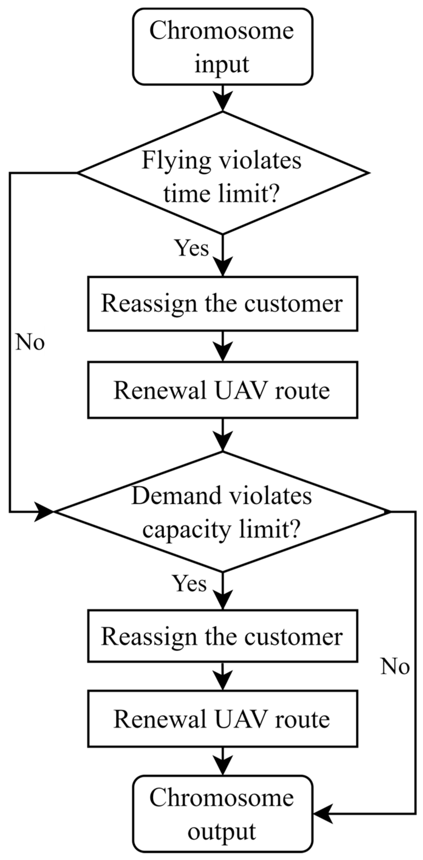
The repair operator plays a crucial role in the HGA, ensuring the diversity and quality of the population. Its task is to adjust solutions that do not meet the constraint conditions (i.e., infeasible chromosomes) so that they satisfy the problem’s actual constraints. In the HGA, we designed a route repair operator.

For the H-G&U IOP problem, the primary goal of the route repair operator is to ensure that each UAV’s route conforms to the constraints regarding demand and flight duration. For those infeasible solutions, the repair operator restores chromosome feasibility by selecting the routes with the highest demand and flight duration and appropriately redistributing nodes between them. This redistribution is accomplished through a series of insertion and deletion operations, as illustrated in Figure 7. For routes that violate the flight duration constraints, the repair operator removes the last customer from the route and reallocates it to the UAV with the shortest flight time; for routes that violate capacity constraints, the operator reallocates the customer to the UAV with the smallest demand.

5. Numerical Experiments and Results

In this section, we conduct numerical experiments using a PC (AMD Ryzen 7-5800H, 2.80 GHz, 16 GB RAM) to validate the effectiveness of our proposed model and the efficiency of our developed solution method. The model is implemented with CPLEX (Version 22.1.1.0) using the concert technology of Python (Version 3.9). The parameter settings are reported in Section 5.1. Section 5.2 presents a comparison between CPLEX and BPA. Section 5.3 reveals the performance of BPA on large-scale instances and its own ablation experiments. Section 5.4 conducts a sensitivity analysis.

5.1. Parameters Setting

Since the mission planning model is similar to the VRP, the parameters for airports, customer locations, and demands in our instances are based on Solomon’s benchmark data [Solomon, 1987]. The customer’s initial value $v_j$ is set to 10. The task execution time $t_j$ for customers is randomly generated, referencing actual application data, and ranges between 11 and 15 min. We categorize all tasks into four types, with the GCR capability values for different customer types being random numbers from {0.7, 0.8, 0.9, 1.0}. The UAVs are classified into two types, carrying resource quantities of 150 and 200, respectively, and their capabilities for the four customer types are {1.0, 1.0, 0.7, 0.7} and {0.7, 0.7, 1.0, 1.0}, respectively, with an endurance of 300 min each. The parameter $\gamma$ for the monotonically decreasing function $\psi (t)$ of customer profit is set to 0.004, and the parameter $\beta$ for the monotonically decreasing function $\phi (t)$ of GCR capability is set to 0.4, as illustrated in Figure 8.

The population size for the HGA is set to 100, with a crossover rate of 0.9, a mutation rate of 0.1, and an elite individual proportion of 3%, totaling three individuals. We observed that for small-scale problems (where the number of customers is fewer than or equal to five), the HGA converges to the optimal value after just one iteration. Therefore, for small-scale problems, the number of iterations for the HGA is set to 1. For problems with more than 10 customers, we set the maximum number of iterations to 300. If the best solution does not improve over 30 consecutive iterations, the algorithm stops and outputs the current best solution. The solving time for BPA is denoted as $T_b$, and the resulting solution is denoted as $Z_b$.

5.2. Comparison between CPELX and BPA

The comparison results between BPA and CPLEX are shown in

Table 2. Performance of the Cplex and the BPA.

Instance ID	Cplex			BPA		GAP (%)	Time Ratio (%)
	${\mathit{T}}_{\mathit{c}}$	${\mathit{Z}}_{\mathit{c}}$	gap	${\mathit{T}}_{\mathit{b}}$	${\mathit{Z}}_{\mathit{b}}$	$({\mathit{Z}}_{\mathit{b}}-{\mathit{Z}}_{\mathit{c}})/{\mathit{Z}}_{\mathit{c}}$	${\mathit{T}}_{\mathit{b}}/{\mathit{T}}_{\mathit{c}}$
A5-2-2-1	1.042	127.682	0	0.066	127.682	0	6.334
A5-2-2-2	1.011	127.338	0	0.044	127.338	0	4.352
A5-2-2-3	0.954	140.003	0	0.100	140.003	0	10.482
A5-2-2-4	0.855	139.334	0	0.055	139.334	0	6.433
A5-2-2-5	0.805	140.754	0	0.042	140.754	0	5.217
A10-2-2-1	739.709	260.666	0	2.093	260.666	0	0.283
A10-2-2-2	7200	259.986	0.030	2.744	259.986	0	0.038
A10-2-2-3	7200	253.417	0.034	4.590	253.417	0	0.064
A10-2-2-4	7200	253.384	0.032	5.267	253.384	0	0.073
A10-2-2-5	4036.055	262.254	0	3.336	262.254	0	0.083
A15-2-2-1	7200	362.205	0.059	8.793	362.663	0.126	0.122
A15-2-2-2	7200	371.221	0.052	3.951	371.467	0.066	0.055
A15-2-2-3	7200	380.975	0.065	4.042	381.158	0.048	0.056
A15-2-2-4	7200	381.928	0.052	3.052	382.568	0.168	0.042
A15-2-2-5	7200	359.471	0.058	5.854	359.796	0.090	0.081
B20-3-3-1	7200	none		7.930	525.222		0.110
B20-3-3-2	7200	509.510	0.082	12.680	526.023	3.241	0.176
B20-3-3-3	7200	none		13.987	494.905		0.194

, which provides the objective values ”$Z$”, computation time “$T$”, Gap = $(Z_b-Z_c)/Z_c$, and Time ratio = $(T_b/T_c)$. Here, $Z_c$ represents the solutions obtained by CPLEX, while $Z_b$ represents the solutions provided by BPA; $T_c$ is the computation time of CPLEX in seconds, and $T_b$ is the computation time of BPA in seconds. We tested four types of instances containing 5, 10, 15, and 20 customers, totaling 16 instances, as shown in Table 2. Each instance ID consists of four parts: the number of customers, the number of GCRs, the number of UAVs, and the instance index. “A” denotes small-scale instances, referring specifically to instances with a number of customers less than 20, while “B” denotes large-scale instances, which are characterized by having 20 or more customers. When the number of customers in instances is “5”, both CPLEX and BPA can obtain the optimal solution, but the average time ratio is 6.564%, demonstrating that BPA solves the problem faster. When the number of customers reaches “10”, for instances 1 and 5, both CPLEX and BPA can achieve the optimal solution, but the average time ratio is 0.183%, indicating that BPA’s solving speed far exceeds that of CPLEX. For instances 2 to 4, CPLEX fails to obtain the optimal solution within two hours, whereas BPA can still quickly find a solution, with results equal to CPLEX. When the number of customers reaches “15”, CPLEX fails to obtain an optimal solution for any instance. In contrast, BPA can achieve solutions that surpass those provided by CPLEX in a remarkably shorter time frame. For all small-scale instances, the average GAP is 0.033%, and the average time ratio is 2.248%. Compared with CPLEX, BPA can obtain better solutions in a shorter time.

Moreover, it can be observed that when facing the three instances with 20 customers, CPLEX is unable to find a feasible solution within two hours for two of these instances. This indicates that CPLEX struggles to solve the proposed MILP model for large-scale instances. However, BPA can still obtain a solution in a relatively short time.

5.3. Performance of the BPA

In scenarios where CPLEX cannot obtain a solution for large-scale instances, our proposed method is capable of providing feasible solutions within a reasonable time frame. As shown in Table 2, we list a total of 36 instances ranging from 20 to 100 customers to test large-scale instances, where the meaning of each instance ID is the same as that in Table 1 for small-scale instances. As depicted in Figure 9, the planning results for each instance include mission planning schemes and a Gantt chart work schedule of GCRs. Additionally, we conducted a comparative experiment to analyze our proposed BPA algorithm, specifically between the version that includes the LS-VND module (Section 4.2.2) and a simplified version without the LS-VND module. Here, $Z_w$ is the solution obtained by the BPA without LS-VND. Time ratio = $T_b/T_w$, where $T_w$ is the computing time of the BPA (without LS-VND) in seconds. From the data in

Table 3. Performance of BPA (without LS-VND) and BPA for large-scale instances.

Instance ID	BPA (without LS-VND)		BPA		GAP (%)	Time Ratio (%)
	${\mathit{T}}_{\mathit{w}}$	${\mathit{Z}}_{\mathit{w}}$	${\mathit{T}}_{\mathit{b}}$	${\mathit{Z}}_{\mathit{b}}$	$({\mathit{Z}}_{\mathit{b}}-{\mathit{Z}}_{\mathit{w}})/{\mathit{Z}}_{\mathit{w}}$	${\mathit{T}}_{\mathit{b}}/{\mathit{T}}_{\mathit{w}}$
B20-3-3-1	7.194	520.552	7.930	525.222	0.897	110.231
B20-3-3-2	15.798	525.002	12.680	526.023	0.194	80.263
B20-3-3-3	13.588	490.848	13.987	494.905	0.827	102.936
B30-4-4-1	18.965	761.740	14.642	768.187	0.846	77.205
B30-4-4-2	22.934	739.484	18.059	741.161	0.227	78.743
B30-4-4-3	20.845	765.430	16.272	769.020	0.469	78.062
B40-6-6-1	33.478	1043.778	24.901	1046.559	0.266	74.380
B40-6-6-2	32.132	996.528	31.234	1002.332	0.582	97.205
B40-6-6-3	37.138	1045.927	25.531	1050.499	0.437	68.746
B50-7-7-1	44.955	1309.581	38.637	1315.082	0.420	85.946
B50-7-7-2	33.399	1303.350	33.010	1307.296	0.303	98.835
B50-7-7-3	48.529	1297.647	39.592	1298.816	0.090	81.584
B60-8-8-1	66.182	1547.255	49.329	1553.338	0.393	74.535
B60-8-8-2	64.289	1544.074	46.435	1553.891	0.636	72.229
B60-8-8-3	54.145	1564.059	53.268	1568.141	0.261	98.380
B70-10-10-1	82.943	1752.441	54.534	1757.855	0.309	65.749
B70-10-10-2	99.410	1827.901	73.357	1832.817	0.269	73.792
B70-10-10-3	73.053	1848.599	67.373	1855.739	0.386	92.225
B80-11-11-1	107.490	2103.974	87.189	2106.567	0.123	81.114
B80-11-11-2	112.642	2078.995	88.608	2083.917	0.237	78.663
B80-11-11-3	113.506	2053.081	93.421	2058.509	0.264	82.305
B90-12-12-1	153.459	2328.142	112.564	2337.002	0.381	73.351
B90-12-12-2	133.998	2384.167	115.896	2388.774	0.193	86.491
B90-12-12-3	135.775	2376.958	108.793	2378.013	0.044	80.127
B100-14-14-1	197.581	2546.527	180.939	2556.122	0.377	91.577
B100-14-14-2	241.909	2634.321	207.048	2637.745	0.130	85.589
B100-14-14-3	231.046	2612.914	214.610	2617.316	0.168	92.886

, we can observe that the BPA solves the problem in a relatively short time. Moreover, in all instances, the LS-VND module significantly accelerates the algorithm’s convergence speed and improves the solution quality. The average time ratio between BPA (without LS-VND) and BPA is 83.82%, and the average gap is 0.36%. As shown in Figure 10a, the average gap for all instances of each scale is greater than 0, with the maximum gap occurring when the instance scale is 20. And the average solving time of BPA is less than that of BPA (without LS-VND) for instances of all scales. For instance, for “B100-14-14-1”, the convergence curves of the two algorithms are shown in Figure 11, where we can observe that LS-VND significantly improves the quality of the initial solution, accelerates the convergence speed, enhances convergence accuracy, and shortens the convergence time.

We also compared the solution quality of the two algorithms under the same time constraints, with the results for nine instances ranging from 80 to 100 customers shown in

Table 4. The performance of BPA (without LS-VND) and BPA in a limited time of 60 s.

Instance ID	BPA (without LS-VND)	BPA	GAP(%)
	${\mathit{Z}}_{\mathit{w}}$	${\mathit{Z}}_{\mathit{b}}$	$({\mathit{Z}}_{\mathit{b}}-{\mathit{Z}}_{\mathit{w}})/{\mathit{Z}}_{\mathit{w}}$	$\mathit{T}(\mathbf{s})$
B80-11-11-1	2101.519	2106.567	0.240	60 s
B80-11-11-2	2076.399	2083.917	0.362	60 s
B80-11-11-3	2049.275	2058.509	0.451	60 s
B90-12-12-1	2317.701	2332.457	0.637	60 s
B90-12-12-2	2378.847	2385.415	0.276	60 s
B90-12-12-3	2373.710	2377.948	0.179	60 s
B100-14-14-1	2541.571	2550.247	0.341	60 s
B100-14-14-2	2631.049	2632.177	0.043	60 s
B100-14-14-3	2609.935	2613.271	0.128	60 s

. The experimental results indicate that the LS-VND module significantly increases the algorithm’s convergence speed and improves the quality of the solutions. The enhancement effect of the LS-VND module is visually evident in Figure 11.

5.4. Sensitivity Analysis

In this section, we primarily analyze parameter $\beta$ of the GCR capability variation function. As shown in

Table 5. Comparison of different $\beta$.

Instance ID	$\mathit{\beta }$	${\mathit{V}}_{\mathit{s}}$	${\mathit{Z}}_{\mathit{s}}$	${\mathit{Z}}_{\mathit{b}}$	${\mathit{Z}}_{\mathit{s}}/{\mathit{Z}}_{\mathit{b}}(\mathit{\%})$
C90-12-12-0	0	550	1532.598	2959.341	51.788
C90-12-12-1	0.1	554	1544.518	2945.629	52.434
C90-12-12-2	0.2	558	1549.825	2918.712	53.100
C90-12-12-3	0.3	561	1557.138	2905.733	53.588
C90-12-12-4	0.4	568	1570.566	2889.076	54.362
C90-12-12-5	0.5	573	1588.130	2865.332	55.426
C90-12-12-6	0.6	577	1590.865	2854.470	55.732
C90-12-12-7	0.7	583	1607.165	2848.278	56.426
C90-12-12-8	0.8	595	1635.993	2827.688	57.856
C90-12-12-9	0.9	595	1634.287	2791.474	58.546

, we set up a total of 10 instances with a customer scale of 90, where $\beta$ ranges from 0 to 0.9. The meaning of each instance ID is the same as that in Table 1 for small-scale instances. Here $V_s$ represents the initial total value of customers served within the first 100 s in the planning scheme. $Z_s$ represents the profit within the first 100 s. Aside from the different $\beta$ parameters, the other parameter information for the 10 instances is entirely consistent. For a straightforward comparison, we set the initial value of customers $v_j$ as random integers between 10 and 15, with other parameter information configured according to the method described in Section 5.1.

According to the data presented in Table 5, we observe that as parameter $\beta$ increases, the total value of customers served within the first 100 s ($V_s$) also increases, along with the profit within the first 100 s ($Z_s$), as illustrated in Figure 12a. This indicates that the faster the decline in GCR’s capability, the more the system tends to prioritize serving high-value customers earlier. Additionally, we note that the overall profit ($Z_b$) for all tasks decreases, while the proportion of profit within the first 100 s ($Z_s/Z_b$) increases, as shown in Figure 12b. This implies that if the degradation effect of GCR’s capability is significant, higher-profit tasks should be allocated to GCR in the initial service phase. It is noteworthy that when $\beta$ = 0.9, the increase in $V_s$ encounters a bottleneck. Our analysis suggests that this is because the advantage of prioritizing high-value customers can no longer offset the losses induced by the decline in GCR’s capability.

6. Discussion

The experimental results demonstrate that for small-scale problems, the quality of solutions obtained by our proposed BPA surpasses those generated by CPLEX after 2 h of computation. Additionally, the average computation time required by our algorithm is only 2.248% of that needed by CPLEX. Moreover, BPA is capable of solving some large-scale problems (100 customers, 14 GCRs, and 14 UAVs) within reasonable computation times. This clearly illustrates the efficacy of BPA in addressing the H-G&U IOP.

Additionally, our method comprehensively considers the capability characteristics of heterogeneous GCRs and the degradation effects of GCR operational abilities during the multi-UAV mission planning phase. This allows for a tighter integration of human and UAV systems, thereby fully leveraging the overall efficiency of the human-machine system. The proposed planning method can yield greater practical profits and holds significant real-world implications.

Future research directions may include the following:

• The model and method proposed in this paper are not only applicable to long-endurance UAVs but also potentially extendable to other multirobot systems, such as multiple unmanned surface vehicles or multiple unmanned ground vehicles;
• The modeling approach for GCR capabilities could be further refined. However, using our model, any form of function can be linearized for a solution;
• In practical applications, unforeseen situations such as dynamic changes in customer demand or UAV malfunctions may arise, necessitating mission replanning. This requires a faster response time, and the speed of existing algorithms for large-scale scenarios may be insufficient. Exploring solutions using deep reinforcement learning methods is worth considering.

7. Conclusions

The primary contributions of this study are as follows: First, we conduct an exploratory investigation into the integrated optimization problem of multi-long-endurance unmanned aerial vehicle (UAV) mission planning and multi-heterogeneous ground control resource assignment (H-G&U IOP). The H-G&U IOP comprehensively considers elements not previously examined in the literature, including the heterogeneity of ground control resources (GCR) and the impact of degradation effects on multi-UAV mission planning, as well as the flexible matching mechanism between GCRs and UAVs. Furthermore, the H-G&U IOP is formulated as a mixed-integer linear programming model aimed at maximizing the profit from completing all tasks. To efficiently solve the proposed model, we present a bi-level programming algorithm (BPA) based on a hybrid genetic algorithm framework. The BPA incorporates heuristic methods such as local search–variable neighborhood descent and a greedy algorithm combined with local search. Subsequently, the effectiveness of the proposed solution method is validated through numerical experiments. Finally, we provide a detailed analysis of the experimental results and discuss potential directions for future research.

8. Patents

A patent application has been filed for the work reported in this manuscript: “Method, Device, and Computer Equipment for Long-Endurance UAV Mission Planning”.