Equivalent Spatial Plane-Based Relative Pose Estimation of UAVs

Abstract

The accuracy of relative pose estimation is an important foundation for ensuring the safety and stability of autonomous aerial refueling (AAR) of unmanned aerial vehicles (UAV), and in response to this problem, a relative pose estimation method of UAVs based on the spatial equivalent plane is proposed in this paper. The UAV is equivalent to a spatial polygonal plane, and according to the measurement information of the Global Navigation Satellite System (GNSS) receivers, the equivalent polygonal plane equation is solved through the three-point normal vector and the minimum sum of squares of the distance from the four points to the plane. The equations of the distance between the geometric centers of the two polygonal planes, the angle between planes, and the angle between lines are used to calculate the relative pose information of the UAVs. Finally, the simulation environment and initial parameters are utilized for numerical simulation and results analysis. The simulation results show that without considering the motion model of the UAV, the proposed method can accurately estimate the relative pose information of the UAVs. In addition, in the presence of measurement errors, the relative pose estimation method based on the equivalent triangle plane can identify the position of the measurement point with the error, and the relative pose estimation method based on the equivalent quadrilateral plane has good robustness. The simulation results verify the feasibility and effectiveness of the proposed method.

1. Introduction

Autonomous aerial refueling technology effectively improves the endurance capacity and air holding time of the UAV and solves problems such as underloading [1]. In the process of AAR, the relative pose information of the UAVs is usually fed back to the controller so that the UAVs can fly under a certain safe distance and at the same altitude to ensure the stability and safety of the refueling process [2,3]; therefore, research on the relative pose estimation method has very important practical significance in ensuring the safety and stability of the AAR process.

At present, the relative pose estimation methods of the UAVs mainly focus on estimation methods based on the global navigation satellite system (GNSS), the inertial navigation system (INS), the vision navigation equipment (VisNav), and their combination [4,5]. The GNSS and INS can directly measure the relative pose parameter information of UAVs; however, the disadvantage of the GNSS is that the signal update frequency is slow and the signal is easily lost due to interference from external factors, while the disadvantage of INS is that the accumulated error leads to lower measurement accuracy, therefore relative pose estimation methods based on GNSS or INS have poor robustness and low estimation accuracy [6,7,8]. VisNav can effectively make up for the shortcomings of GNSS or INS and improve the accuracy of relative pose estimations [9]. Campa et al. [10] used a camera installed on a UAV to observe feature points on another UAV with a known location and established a relative line-of-sight vector equation to solve the relative pose between the camera and the UAV. Mammarella and Fravolini [11,12] set a series of dot-shaped marker lights on a tanker as auxiliary identification markers and then extracted and tracked these marker points, using iterative algorithms such as the Gauss–Newton method to estimate the relative pose information. Ding et al. [13] discussed the application of the orthogonal iteration (OI) algorithm in AAR and analyzed the influence of the number of marker points and layout on the accuracy of relative pose estimation. Doebbler et al. [14] used the active variable contour algorithm to extract rectangular markers set on the nose and achieved relative pose estimation by tracking the centroid of the rectangular markers. Zhang et al. [15,16] established an optimization method based on the geometric information between stereo vision and the target object to measure the pose of the spatial craft and obtain the altitude solution of the non-cooperative target. Hinterstoisser et al. [17] estimated the target pose information by matching the real image with the viewpoint production template, set the threshold, obtained the ideal matching result, and completed the pose estimation by matching the real image with the obtained sample template, including the color and depth gradient from different angles. Weaver et al. [18] compared the predicted image of the tanker with the actual measured image and used the obtained image error and inertial navigation system data for fusion calculation to obtain the relative pose information. Li Guorong [19] back-calculated and estimated the target flight attitude by comparing the simulated image and real image, while the target attitude parameters were determined using the pyramid area-matching algorithm and the external contour point set matching was used to optimize the iterative algorithm. Liebelt et al. [20] used the target contour-matching method to calculate the deviation between the reprojection result and the actual imaging result of the target edge with a given initial value, and then iterative optimization minimized the deviation to achieve the target pose solution. In a long-distance situation, Teng et al. [21] used two cameras to extract and cluster image line features and solve the altitude of the helicopter under geometric constraints. Under the constraints of single-view and multi-view UAVs, Yuan et al. [22] established a particle filter algorithm based on multiple cameras to estimate the pose information of the UAV, which improved the estimation accuracy. However, the relative pose estimation method based on VisNav needs to know the parameters of the camera and UAV model in advance, while at the same time, there are measurement and quantization errors in the actual imaging process and extraction errors in the feature extraction process, which will affect the estimation accuracy of the relative pose. In addition, this method usually transforms the position and altitude into the same objective function and iteratively solves the optimal solution, which requires a large amount of calculation and affects the real-time performance of the method. Because of the shortcomings and deficiencies of a single system/device, a relative pose estimation method based on multiple measurement systems/devices has been proposed and studied. Williamson et al. [23] established a relative navigation method based on INS/GPS for the formation flight of UAVs, but when the GPS signal was interfered with, the accuracy of relative navigation was reduced. Strohmeier et al. [24] proposed a relative pose estimation method of the UAVs based on GPS/MEMS IMU but the estimation accuracy was affected by the cumulative error of the IMU. Christian et al. [25] proposed a relative pose estimation method of light UAVs based on GPS/MEMS IMU, but the estimation accuracy was affected by the stability of the GPS signal and the cumulative errors of the IMU. Fosbury [26], Shao Wei [27], and Wang Long [28] researched the relative navigation information method of UAVs based on VisNav/INS. They used the image obtained by the camera to calculate the relative pose information of UAVs and correct the errors caused by the INS, and this method improved the accuracy of relative navigation. However, when the field of view was occluded, VisNav was not able to observe the feature points so the relative pose information could not be correctly calculated, which affected the accuracy of relative navigation. However, most existing methods require the establishment of accurate system models. Considering the complexity and bias of the motion model of the tanker/receiver, as well as the computational complexity of model-based methods, a relative pose estimation method of UAVs based on the spatial equivalent plane is proposed in this paper. The proposed method equates the UAV to a spatial polygonal plane and uses the relative distance and angle between the equivalent polygonal planes to solve the relative pose information of the UAVs.

The structure of this paper is as follows. The spatial equivalent triangle plane equation of the UAV based on the three-point normal vector and the spatial equivalent quadrilateral plane equation of the UAV based on the minimum square sums of the distance from the four points to the plane are determined, and the relative pose of the UAV is solved in Section 2; initial simulation parameters are configured to verify the proposed method and analyze the simulation results in Section 3; finally, conclusions are drawn in Section 4.

2. Relative Pose Estimation Method of UAVs

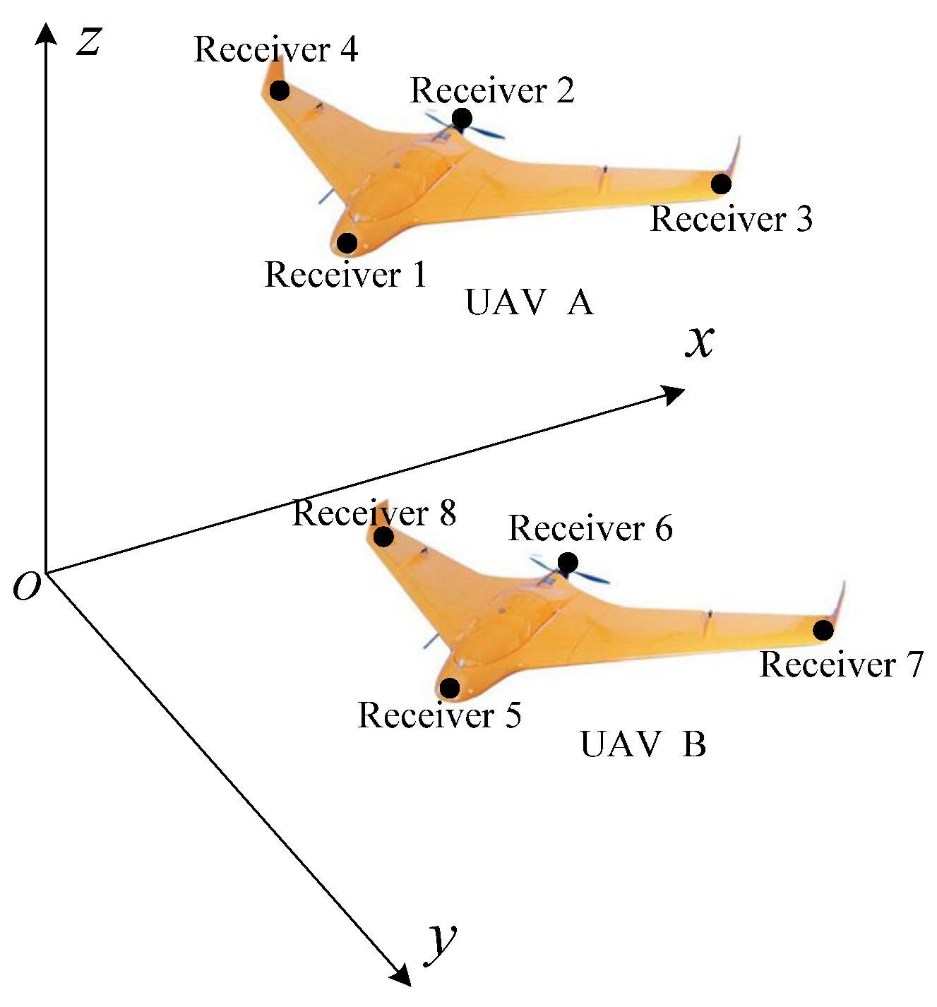
2.1. Problem Description

In this paper, when we research the relative pose estimation of the UAVs, the UAV is described as a spatial equivalent polygonal plane, and the problem of solving the relative pose estimation between UAVs is transformed into the problem of solving the relative distance and angle between two spatial equivalent polygonal planes in the same coordinate system. Taking the Earth-Centered, Earth-Fixed (ECEF) system as the reference coordinate system and the fixed-wing UAV as the research object, GNSS receivers are installed on the nose, tail, and two wings of the UAV to receive a satellite navigation signal and realize the single-receiver positioning, and then the positioning information of the GNSS receivers is used to determine the spatial equivalent polygonal plane equation of the UAV and calculate the relative position and angle between the spatial equivalent polygonal planes. Finally, we can obtain the relative pose information of the UAVs. The schematic diagram of relative pose estimation is shown in Figure 1.

2.2. Determination of Spatial Equivalent Polygon Plane Equation

Taking the ECEF as the reference coordinate system, the measured value of the GNSS receiver installed on the UAV is P_n = (x_n, y_n, z_n), (n = 1, 2,…, 8), where each UAV is equivalent to a spatial polygonal plane. When the measured values of four points on each UAV are known, we can use three points to determine a triangle plane or four points to determine a quadrilateral plane; therefore, the spatial triangle plane equation based on the three-point normal vector and the spatial quadrilateral plane based on the minimum square sum of the distance from the four points to the plane will be discussed in this section.

2.2.1. Three Points to Determine the Spatial Triangle Plane

For UAV A, when the measurement values of the GNSS receivers are known, any three measurement values can be used to determine the equivalent spatial triangle plane equation of UAV A. According to the three measurement values, the normal vector ${\overrightarrow{n}}_A$ of the equivalent spatial triangle plane is:

$${\overrightarrow{n}}_A=\overrightarrow{P_i{P}_j}\times \overrightarrow{P_i{P}_k}=\left(\left(L_3{L}_6-L_4{L}_5\right),\left(L_5{L}_2-L_6{L}_1\right),\left(L_1{L}_4-L_2{L}_3\right)\right)$$

(1)

where L₁ = x_j − x_i, L₂ = x_k − x_i, L₃ = y_j − y_i, L₄ = y_k − y_i, L₅ = z_j − z_i, and L₆ = z_k − z_i, while the values of i, j, and k are (i = 1, j = 2, k = 3), (i = 1, j = 2, k = 4), (i = 1, j = 3, k = 4), and (i = 2, j = 3, k = 4).

The point normal form equation of a spatial plane is:

$$a\left(x-x_0\right)+b\left(y-y_0\right)+c\left(z-z_0\right)=0$$

(2)

where (a, b, c) represents the normal vector and (x₀, y₀, z₀) represents the known point.

When the normal vector is known, if the equivalent spatial triangle plane of UAV A passes through the origin of the reference coordinate system, that is, point (0, 0, 0), the equation of the spatial triangle plane is:

$$\left(L_3{L}_6-L_4{L}_5\right)x+\left(L_5{L}_2-L_6{L}_1\right)y+\left(L_1{L}_4-L_2{L}_3\right)z=0$$

(3)

If the equivalent spatial triangle plane of UAV A does not pass through the origin of the reference coordinate system, at this time, point P_n = (x_n, y_n, z_n), (n = i, j, k) can be taken as the known point. Then, the equation of the spatial triangle plane is:

$$\left(L_3{L}_6-L_4{L}_5\right)\left(x-x_n\right)+\left(L_5{L}_2-L_6{L}_1\right)\left(y-y_n\right)+\left(L_1{L}_4-L_2{L}_3\right)\left(z-z_n\right)=0$$

(4)

Similarly, for UAV B, the normal vector ${\overrightarrow{n}}_B$ of the spatial triangle plane determined by any three points on the aircraft is:

$${\overrightarrow{n}}_B=\overrightarrow{R_l{R}_q}\times \overrightarrow{R_l{R}_w}=\left(\left(M_3{M}_6-M_4{M}_5\right),\left(M_5{M}_2-M_6{M}_1\right),\left(M_1{M}_4-M_2{M}_3\right)\right)$$

(5)

where M₁ = x_q − x_l, M₂ = x_w − x_l, M₃ = y_q − y_l, M₄ = y_w − y_l, M₅ = z_q − z_l, and M₆ = z_w − z_l, while the values of l, q, and w are (l = 5, q = 6, w = 7), (l = 5, q = 6, w = 8), (l = 5, q = 7, w = 8), and (l = 6, q = 7, w = 8).

When the normal vector is known, if the equivalent spatial triangle plane of UAV B passes through the origin of the reference coordinate system, that is, point (0, 0, 0), the equation of the spatial triangle plane is:

$$\left(M_3{M}_6-M_4{M}_5\right)x+\left(M_5{M}_2-M_6{M}_1\right)y+\left(M_1{M}_4-M_2{M}_3\right)z=0$$

(6)

If the equivalent spatial triangle plane of UAV B does not pass through the origin of the reference coordinate system, at this time, point P_n = (x_n, y_n, z_n), (n = l, q, w) can be taken as the known point. Then, the equation of the spatial triangle plane is:

$$\left(M_3{M}_6-M_4{M}_5\right)\left(x-x_n\right)+\left(M_5{M}_2-M_6{M}_1\right)\left(y-y_n\right)+\left(M_1{M}_4-M_2{M}_3\right)\left(z-z_n\right)=0$$

(7)

2.2.2. Four Points to Determine the Spatial Quadrilateral Plane

In the previous section, the three-point normal vector is used to determine the spatial triangle plane equation. In this section, the four points on the UAV will be used to determine the equivalent spatial quadrilateral plane equation of the UAV. Assuming that the equivalent spatial quadrilateral plane equation of the UAV A is:

$$e_{A}x+f_{A}y+g_{A}z=d_A$$

(8)

where (e_A, f_A, g_A) is the normal vector and dA is the dot product of the normal vector value and the known point value.

The minimum sum of the squares of distances from the point to the spatial plane is used to determine the spatial quadrilateral plane equation. The distance from the measurement points to the spatial quadrilateral plane is:

$$r_{An}={\displaystyle \frac{\left|e_A{x}_n+f_A{y}_n+g_A{z}_n-d_A\right|}{\sqrt{e_A^2+f_A^2+g_A^2}}}(n=1,2,3,4)$$

(9)

In order to minimize the sum of the squares of distances from four points on UAV A to the equivalent spatial quadrilateral plane, we define an object function J(e_A, f_A, g_A, d_A):

$$J\left(e_A,f_A,g_A,d_A\right)={\displaystyle \sum _{n=1}^4{\left(\frac{\left|x_n{e}_A+y_n{f}_A+z_n{g}_A-d_A\right|}{\sqrt{e_A^2+f_A^2+g_A^2}}\right)}^2}$$

(10)

Equation (10) is a nonlinear function. To find the optimal solution, the Gauss–Newton method can be used to iteratively calculate the linear optimal solution.

Let $J_n={\left({\displaystyle \frac{\left|x_n{e}_A+y_n{f}_A+z_n{g}_A-d_A\right|}{\sqrt{e_A^2+f_A^2+g_A^2}}}\right)}^2$, (n = 1, 2, 3, 4), the partial derivative is:

$$\{\begin{array}{l}{\displaystyle \frac{\partial J_n}{\partial e_A}}=2{\displaystyle \frac{x_n\left|x_n{e}_A+y_n{f}_A+z_n{g}_A-d_A\right|-e_A{\left|x_n{e}_A+y_n{f}_A+z_n{g}_A-d_A\right|}^2}{{\left(e_A^2+f_A^2+g_A^2\right)}^2}}\\ {\displaystyle \frac{\partial J_n}{\partial f_A}}=2{\displaystyle \frac{y_n\left|x_n{e}_A+y_n{f}_A+z_n{g}_A-d_A\right|-f_A{\left|x_n{e}_A+y_n{f}_A+z_n{g}_A-d_A\right|}^2}{{\left(e_A^2+f_A^2+g_A^2\right)}^2}}\\ {\displaystyle \frac{\partial J_n}{\partial g_A}}=2{\displaystyle \frac{z_n\left|x_n{e}_A+y_n{f}_A+z_n{g}_A-d_A\right|-g_A{\left|x_n{e}_A+y_n{f}_A+z_n{g}_A-d_A\right|}^2}{{\left(e_A^2+f_A^2+g_A^2\right)}^2}}\\ {\displaystyle \frac{\partial J_n}{\partial d_A}}=2{\displaystyle \frac{-\left|x_n{e}_A+y_n{f}_A+z_n{g}_A-d_A\right|}{\left(e_A^2+f_A^2+g_A^2\right)}}\end{array}$$

(11)

According to the results, the Jacobian matrix H_A can be obtained:

$$H_A={\displaystyle \frac{\partial J_n}{\partial \left(e_A,f_A,g_A,d_A\right)}},\left(n=1,2,3,4\right)$$

(12)

Let α_A = (e_A, f_A, g_A, d_A)^T, and select ζ_A as the iteration variable, while the Gauss–Newton method is used for iterative calculation.

$${\alpha }_A^{m+1}={\alpha }_A^m-{\left(H_A^T{H}_A\right)}^{-1}{H}_A^T{\zeta }_A^m,(m=0,1,2,\dots )$$

(13)

where m is the iteration number.

Substituting the final iterative calculation result into Equation (8), we can obtain the equivalent spatial quadrilateral plane equation of UAV A.

Similarly, we assume that the equivalent spatial quadrilateral plane equation of UAV B is:

$$e_{B}x+f_{B}y+g_{B}z=d_B$$

(14)

where (e_B, f_B, g_B) represents the normal vector and d_B is the dot product of the normal vector value and the known point value.

Defining the object function J(e_B, f_B, g_B, d_B):

$$J\left(e_B,f_B,g_B,d_B\right)={\displaystyle \sum _{n=5}^8{\left(\frac{\left|x_n{e}_B+y_n{f}_B+z_n{g}_B-d_B\right|}{\sqrt{e_B^2+f_B^2+g_B^2}}\right)}^2}$$

(15)

Calculating the partial derivative of the Equation (15), the Jacobian matrix H_B is:

$$H_B={\displaystyle \frac{\partial J_n}{\partial \left(e_B,f_B,g_B,d_B\right)}},\left(n=5,6,7,8\right)$$

(16)

Let α_B = (e_B, f_B, g_B, d_B)^T, and select ζ_B as the iteration variable, while the Gauss–Newton method is used for iterative calculation.

$${\alpha }_B^{m+1}={\alpha }_B^m-{\left({H_B}^T{H}_B\right)}^{-1}{H_B}^T{\zeta }_B^m,\left(m=0,1,2,\cdots \right)$$

(17)

Substituting the final iterative calculation result into Equation (11), we can obtain the equivalent spatial quadrilateral plane equation of UAV B.

2.3. Relative Pose Estimation of UAVs

The pose of the UAV is constantly changing during flight, and the accurate estimation of the relative pose of the UAV is the prerequisite and basis for multiple UAVs to complete coordinated control tasks. In this paper, the UAV is equivalent to a spatial polygonal plane, therefore the problem of the relative pose between UAVs is transformed into a problem of the relative position and angle between polygonal planes. We can define the distance between the geometric center of the spatial polygon planes as the relative distance r_rel between UAVs, the angle between the normal vectors of the spatial polygon planes as the relative angle φ_rel between UAVs, the angle between the straight lines formed by the nose and tail of the UAVs as the relative angle θ_rel between the UAVs, and the angle between the straight lines formed by the two wings of the UAVs as the relative angle ψ_rel between the UAVs. When the normal vectors of the equivalent spatial polygonal planes of the UAVs and the measurement values of the GNSS receivers on the UAV are known, we can calculate the relative pose information of the UAVs.

The relative distance r_rel between the UAVs can be solved by calculating the relative distance between the geometric centers of the equivalent spatial polygonal planes. When the measurement values of the GNSS receivers are known, the geometric center position coordinates O_A and O_B of the equivalent spatial polygon planes of UAV A and B are, respectively:

$$\{\begin{array}{l}{O}_A={\displaystyle \frac{1}{N}}\left({\displaystyle \sum _{n=1}^N{x}_n},{\displaystyle \sum _{n=1}^N{y}_n},{\displaystyle \sum _{n=1}^N{z}_n}\right)\\ O_B={\displaystyle \frac{1}{N}}\left({\displaystyle \sum _{s=1}^N{x}_s},{\displaystyle \sum _{s=1}^N{y}_s},{\displaystyle \sum _{s=1}^N{z}_s}\right)\end{array}$$

(18)

where N is the number of the GNSS receiver, and in this paper, N is 3 or 4.

According to the results of Equation (18), the relative distance r_rel is:

$$r_{rel}=\left|O_A{O}_B\right|={\displaystyle \frac{1}{N}}\sqrt{{\left({\displaystyle \sum _{s=1,n=1}^N\left(x_s-x_n\right)}\right)}^2+{\left({\displaystyle \sum _{s=1,n=1}^N\left(y_s-y_n\right)}\right)}^2+{\left({\displaystyle \sum _{s=1,n=1}^N\left(z_s-z_n\right)}\right)}^2}$$

(19)

When the normal vectors of the spatial polygon planes are known, the relative angle φ_rel between the equivalent spatial triangle planes is:

$$\begin{array}{cc}\hfill {\varphi }_{rel}& =\arccos {\displaystyle \frac{\left|{\overrightarrow{n}}_A{\overrightarrow{n}}_B\right|}{\left|{\overrightarrow{n}}_A\right|\left|{\overrightarrow{n}}_B\right|}}\hfill \\ & =\arccos {\displaystyle \frac{\left(L_3{L}_6-L_4{L}_5\right)\left(M_3{M}_6-M_4{M}_5\right)+\left(L_5{L}_2-L_6{L}_1\right)\left(M_5{M}_2-M_6{M}_1\right)+\left(L_1{L}_4-L_2{L}_3\right)\left(M_1{M}_4-M_2{M}_3\right)}{\sqrt{{\left(L_3{L}_6-L_4{L}_5\right)}^2+{\left(L_5{L}_2-L_6{L}_1\right)}^2+{\left(L_1{L}_4-L_2{L}_3\right)}^2}\sqrt{{\left(M_3{M}_6-M_4{M}_5\right)}^2+{\left(M_5{M}_2-M_6{M}_1\right)}^2+{\left(M_1{M}_4-M_2{M}_3\right)}^2}}}\hfill \end{array}$$

(20)

The relative angle φ_rel between the equivalent spatial quadrilateral planes is:

$${\varphi }_{rel}=\arccos {\displaystyle \frac{\left|e_A{e}_B+f_A{f}_B+g_A{g}_B\right|}{\sqrt{{e_A}^2+{f_A}^2+{g_A}^2}\sqrt{{e_B}^2+{f_B}^2+{g_B}^2}}}$$

(21)

The measurement values of the nose and tail of UAV A are P₁ and P₂, respectively, and the measurement values of the nose and tail of UAV B are P₅ and P₆, respectively, so the relative angle θ_rel is:

$${\theta }_{rel}=\arccos {\displaystyle \frac{\left|\overrightarrow{P_1{P}_2}\cdot \overrightarrow{P_5{P}_6}\right|}{\left|\overrightarrow{P_1{P}_2}\right|\left|\overrightarrow{P_5{P}_6}\right|}}=\arccos {\displaystyle \frac{\left(x_2-x_1\right)\left(x_6-x_5\right)+\left(y_2-y_1\right)\left(y_6-y_5\right)+\left(z_2-z_1\right)\left(z_6-z_5\right)}{\sqrt{{\left(x_2-x_1\right)}^2+{\left(y_2-y_1\right)}^2+{\left(z_2-z_1\right)}^2}\sqrt{{\left(x_6-x_5\right)}^2+{\left(y_6-y_5\right)}^2+{\left(z_6-z_5\right)}^2}}}$$

(22)

The measurement values of the nose and tail of UAV A are P₃ and P₄, respectively, and the measurement values of the nose and tail of UAV B are P₇ and P₈, respectively, so the relative angle ψ_rel is:

$${\psi }_{rel}=\arccos {\displaystyle \frac{\left|\overrightarrow{P_3{P}_4}\cdot \overrightarrow{P_7{P}_8}\right|}{\left|\overrightarrow{P_3{P}_4}\right|\left|\overrightarrow{P_7{P}_8}\right|}}=\arccos {\displaystyle \frac{\left(x_4-x_3\right)\left(x_8-x_7\right)+\left(y_4-y_3\right)\left(y_8-y_7\right)+\left(z_4-z_3\right)\left(z_8-z_7\right)}{\sqrt{{\left(x_4-x_3\right)}^2+{\left(y_4-y_3\right)}^2+{\left(z_4-z_3\right)}^2}\sqrt{{\left(x_8-x_7\right)}^2+{\left(y_8-y_7\right)}^2+{\left(z_8-z_7\right)}^2}}}$$

(23)

According to the results of Equations (19)–(23), we can obtain the relative pose information of the UAVs.

Based on the above deduction and analysis, the steps for solving the relative attitude are as follows:

Step 1: Use data P₁, P₂, P₃, and P₄ from UAV A to calculate the plane normal vector ${\overrightarrow{n}}_A$ and then use the plane equation to obtain the equivalent plane of UAV A.

Step 2: Use data P₅, P₆, P₇, and P₈ from UAV B to calculate the normal vector ${\overrightarrow{n}}_B$ on the plane and then use the plane equation to obtain the equivalent plane of UAV B.

Step 3: Calculate the angle between two equivalent planes to obtain the relative attitude angle φ_rel.

Step 4: Calculate the relative attitude angle θ_rel using data P₁, P₂, P₅, and P₆.

Step 5: Calculate the relative attitude angle ψ_rel using data P₃, P₄, P₇, and P₈.

2.4. Influence of Measurement Error on Estimation Results

The GNSS receivers will have measured errors during the measurement process and affect the accuracy of the relative pose estimation. In this section, we will use the error analysis method to evaluate the estimation results. Assuming that the measurement value P_u (u = 1, 2,..., n) of the GNSS receivers on UAV A has a measurement error of Δ = (Δx, Δy, Δz), according to Equations (18) and (19), we can obtain:

$$\Delta r_{rel}={\displaystyle \frac{\left({\displaystyle \sum _{s=1,n=1}^N\left(x_n-x_s\right)}\right)\Delta x_u+\left({\displaystyle \sum _{s=1,n=1}^N\left(y_n-y_s\right)}\right)\Delta y_u+\left({\displaystyle \sum _{s=1,n=1}^N\left(z_n-z_s\right)}\right)\Delta z_u}{N\sqrt{{\left({\displaystyle \sum _{s=1,n=1}^N\left(x_s-x_n\right)}\right)}^2+{\left({\displaystyle \sum _{s=1,n=1}^N\left(y_s-y_n\right)}\right)}^2+{\left({\displaystyle \sum _{s=1,n=1}^N\left(z_s-z_n\right)}\right)}^2}}}$$

(24)

where Δr_rel is the difference between the current moment and the previous moment of the relative position estimation and (Δx_u, Δy_u, Δz_u) is the difference between the current moment and the previous moment of the measurement value P_u.

Substituting the measurement error of the measured value P_u into Equation (24), we can obtain:

$$\Delta r_{rel}={\displaystyle \frac{\left({\displaystyle \sum _{s=1,n=1}^N\left(x_n-x_s\right)}+\Delta x\right)\Delta x_u+\left({\displaystyle \sum _{s=1,n=1}^N\left(y_n-y_s\right)}+\Delta y\right)\Delta y_u+\left({\displaystyle \sum _{s=1,n=1}^N\left(z_n-z_s\right)}+\Delta z\right)\Delta z_u}{N\sqrt{{\left({\displaystyle \sum _{s=1,n=1}^N\left(x_s-x_n\right)}-\Delta x\right)}^2+{\left({\displaystyle \sum _{s=1,n=1}^N\left(y_s-y_n\right)}-\Delta y\right)}^2+{\left({\displaystyle \sum _{s=1,n=1}^N\left(z_s-z_n\right)}-\Delta z\right)}^2}}}$$

(25)

Equation (25) gives the relationship between the measurement error and the estimation difference in the relative position. It shows that the measurement error will inevitably affect the estimation accuracy of the relative distance and make the estimation result larger or smaller.

For the relative angle φ_rel between the equivalent polygonal planes of the UAVs, if the measured value Pi exists with measurement error, we can obtain:

$$\begin{array}{cc}\hfill \Delta {\varphi }_{rel}& ={\displaystyle \frac{\left(E_1{F}_1+E_2{F}_2+E_3{F}_3\right)E^{2}F\left[E_2\left(L_6-L_5\right)+E_3\left(L_3-L_4\right)\right]-\left[\left(L_6-L_5\right)F_2+\left(L_3-L_4\right)F_3\right]F}{\sqrt{E^5{F}^4-E^3{F}^2{\left(E_1{F}_1+E_2{F}_2+E_3{F}_3\right)}^2}}}\Delta x_i+\hfill \\ & {\displaystyle \frac{\left(E_1{F}_1+E_2{F}_2+E_3{F}_3\right)E^{2}F\left[E_1\left(L_5-L_6\right)+E_3\left(L_2-L_1\right)\right]-\left[\left(L_5-L_6\right)F_2+\left(L_2-L_1\right)F_3\right]F}{\sqrt{E^5{F}^4-E^3{F}^2{\left(E_1{F}_1+E_2{F}_2+E_3{F}_3\right)}^2}}}\Delta y_i+\hfill \\ & {\displaystyle \frac{\left(E_1{F}_1+E_2{F}_2+E_3{F}_3\right)E^{2}F\left[E_1\left(L_4-L_3\right)+E_2\left(L_1-L_2\right)\right]-\left[\left(L_4-L_3\right)F_2+\left(L_1-L_2\right)F_3\right]F}{\sqrt{E^5{F}^4-E^3{F}^2{\left(E_1{F}_1+E_2{F}_2+E_3{F}_3\right)}^2}}}\Delta z_i\hfill \end{array}$$

(26)

where $E_1=\left(L_3{L}_6-L_4{L}_5\right)$, $E_2=\left(L_5{L}_2-L_6{L}_1\right)$, $E_3=\left(L_1{L}_4-L_2{L}_3\right)$, $E=\sqrt{{E_1}^2+{E_2}^2+{E_3}^2}$, $F_1=\left(M_3{M}_6-M_4{M}_5\right)$, $F_2=\left(M_5{M}_2-M_6{M}_1\right)$, $F_3=\left(M_1{M}_4-M_2{M}_3\right)$, and $F=\sqrt{{F_1}^2+{F_2}^2+{F_3}^2}$.

Substituting the measurement error of the measured value P_i into Equation (26), we can obtain:

$$\begin{array}{l}\Delta {\varphi }_{rel}=\\ {\displaystyle \frac{\left[G+\Delta x\left(\left(L_6-L_5\right)F_2+\left(L_3-L_4\right)F_3\right)\right]E^{2}F\left[E_2\left(L_6-L_5\right)+E_3\left(L_3-L_4\right)+\Delta x\left({\left(L_6-L_5\right)}^2+{\left(L_3-L_4\right)}^2\right)\right]-\left[\left(L_6-L_5\right)F_2+\left(L_3-L_4\right)F_3\right]F}{\sqrt{E^5{F}^4-E^3{F}^2{\left(G+\Delta x\left(\left(L_6-L_5\right)F_2+\left(L_3-L_4\right)F_3\right)\right)}^2}}}\Delta x_i\\ +{\displaystyle \frac{\left[G+\Delta y\left(\left(L_5-L_6\right)F_2+\left(L_2-L_1\right)F_3\right)\right]E^{2}F\left[E_1\left(L_5-L_6\right)+E_3\left(L_2-L_1\right)+\Delta y\left({\left(L_5-L_6\right)}^2+{\left(L_2-L_1\right)}^2\right)\right]-\left[\left(L_5-L_6\right)F_2+\left(L_2-L_1\right)F_3\right]F}{\sqrt{E^5{F}^4-E^3{F}^2{\left(G+\Delta y\left(\left(L_5-L_6\right)F_2+\left(L_2-L_1\right)F_3\right)\right)}^2}}}\Delta y_i\\ +{\displaystyle \frac{\left[G+\Delta z\left(\left(L_4-L_3\right)F_2+\left(L_1-L_2\right)F_3\right)\right]E^{2}F\left[E_1\left(L_4-L_3\right)+E_2\left(L_1-L_2\right)+\Delta z\left({\left(L_4-L_3\right)}^2+{\left(L_1-L_2\right)}^2\right)\right]-\left[\left(L_4-L_3\right)F_2+\left(L_1-L_2\right)F_3\right]F}{\sqrt{E^5{F}^4-E^3{F}^2{\left(G+\Delta z\left(\left(L_4-L_3\right)F_2+\left(L_1-L_2\right)F_3\right)\right)}^2}}}\Delta z_i\end{array}$$

(27)

where $G=\left(E_1{F}_1+E_2{F}_2+E_3{F}_3\right)$.

If the measured value P_j exists with measurement error, we can obtain:

$$\begin{array}{cc}\hfill \Delta {\varphi }_{rel}& ={\displaystyle \frac{GF\left(L_1{E}_3-L_6{E}_2\right)-E^{2}F\left(L_4{F}_3-L_6{F}_2\right)}{\sqrt{E^5{F}^4-E^3{F}^2{G}^2}}}\Delta x_j+{\displaystyle \frac{GF\left(L_6{E}_1-L_2{E}_3\right)-E^{2}F\left(L_6{F}_1-L_2{F}_3\right)}{\sqrt{E^5{F}^4-E^3{F}^2{G}^2}}}\Delta y_i+\hfill \\ & {\displaystyle \frac{GF\left(L_2{E}_2-L_4{E}_1\right)-E^{2}F\left(L_2{F}_2-L_4{F}_1\right)}{\sqrt{E^5{F}^4-E^3{F}^2{G}^2}}}\Delta z_i\hfill \end{array}$$

(28)

Substituting the measurement error of the measured value P_j into Equation (28), we can obtain:

$$\begin{array}{l}\Delta {\varphi }_{rel}={\displaystyle \frac{GF\left[L_1{E}_3-L_6{E}_2+\Delta x\left(L_1{L}_4+E_3+L_6^2\right)+{\left(\Delta x\right)}^2{L}_4\right]-E^{2}F\left(L_4{F}_3-L_6{F}_2\right)}{\sqrt{E^5{F}^4-E^3{F}^2{G}^2}}}\Delta x_j+\\ {\displaystyle \frac{GF\left[L_6{E}_1-L_2{E}_3+\Delta y\left(L_2^2+L_6^2\right)\right]-E^{2}F\left(L_6{F}_1-L_2{F}_3\right)}{\sqrt{E^5{F}^4-E^3{F}^2{G}^2}}}\Delta y_i+{\displaystyle \frac{GF\left[L_2{E}_2-L_4{E}_1+\Delta z\left(L_2{L}_5+L_4^2\right)\right]-E^{2}F\left(L_2{F}_2-L_4{F}_1\right)}{\sqrt{E^5{F}^4-E^3{F}^2{G}^2}}}\Delta z_i\end{array}$$

(29)

According to the results of Equations (26)–(28), the measurement error can affect the estimation results of the relative angle φ_rel between the equivalent polygonal planes to a certain extent, and the size of the error affects the deviation of the estimation result.

If the measured value P₁ exists with measurement error, according to Equations (22)–(23), we can obtain:

$$\Delta {\theta }_{rel}={\displaystyle \frac{U\left(V_1\Delta x_1+V_2\Delta y_1+V_3\Delta z_1\right)-V\left(U_1{V}_1+U_2{V}_2+U_3{V}_3\right)\left(U_1\Delta x_1+U_2\Delta y_1+U_3\Delta z_1\right)}{\sqrt{U^4\left[V^2-{\left(U_1{V}_1+U_2{V}_2+U_3{V}_3\right)}^2\right]}}}$$

(30)

where $U_1=\left(x_2-x_1\right)$, $U_2=\left(y_2-y_1\right)$, $U_3=\left(z_2-z_1\right)$, $U=\sqrt{{U_1}^2+{U_2}^2+{U_3}^2}$, $V_1=\left(x_6-x_5\right)$, $V_2=\left(y_6-y_5\right)$, $V_3=\left(z_6-z_5\right)$, and $V=\sqrt{{V_1}^2+{V_2}^2+{V_3}^2}$.

Substituting the measurement error of the measured value P₁ into Equation (30), we can obtain:

$$\begin{array}{c}\Delta {\theta }_{rel}={\displaystyle \frac{\sqrt{{\left(U_1-\Delta x\right)}^2+{\left(U_2-\Delta y\right)}^2+{\left(U_3-\Delta z\right)}^2}\left(V_1\Delta x_1+V_2\Delta y_1+V_3\Delta z_1\right)}{\sqrt{{\left[{\left(U_1-\Delta x\right)}^2+{\left(U_2-\Delta y\right)}^2+{\left(U_3-\Delta z\right)}^2\right]}^2\left[V^2-{\left(\left(U_1-\Delta x\right)V_1+\left(U_2-\Delta y\right)V_2+\left(U_3-\Delta z\right)V_3\right)}^2\right]}}}-\\ {\displaystyle \frac{V\left(\left(U_1-\Delta x\right)V_1+\left(U_2-\Delta y\right)V_2+\left(U_3-\Delta z\right)V_3\right)\left(\left(U_1-\Delta x\right)\Delta x_1+\left(U_2-\Delta y\right)\Delta y_1+\left(U_3-\Delta z\right)\Delta z_1\right)}{\sqrt{{\left[{\left(U_1-\Delta x\right)}^2+{\left(U_2-\Delta y\right)}^2+{\left(U_3-\Delta z\right)}^2\right]}^2\left[V^2-{\left(\left(U_1-\Delta x\right)V_1+\left(U_2-\Delta y\right)V_2+\left(U_3-\Delta z\right)V_3\right)}^2\right]}}}\end{array}$$

(31)

In the same way, we can obtain:

$$\begin{array}{c}\Delta {\psi }_{rel}={\displaystyle \frac{\sqrt{{\left(W_1-\Delta x\right)}^2+{\left(W_2-\Delta y\right)}^2+{\left(W_3-\Delta z\right)}^2}\left(Q_1\Delta x_1+Q_2\Delta y_1+Q_3\Delta z_1\right)}{\sqrt{{\left[{\left(W_1-\Delta x\right)}^2+{\left(W_2-\Delta y\right)}^2+{\left(W_3-\Delta z\right)}^2\right]}^2\left[Q^2-{\left(\left(W_1-\Delta x\right)Q_1+\left(W_2-\Delta y\right)Q_2+\left(W_3-\Delta z\right)Q_3\right)}^2\right]}}}-\\ {\displaystyle \frac{Q\left(\left(W_1-\Delta x\right)Q_1+\left(W_2-\Delta y\right)Q_2+\left(W_3-\Delta z\right)Q_3\right)\left(\left(W_1-\Delta x\right)\Delta x_1+\left(W_2-\Delta y\right)\Delta y_1+\left(W_3-\Delta z\right)\Delta z_1\right)}{\sqrt{{\left[{\left(W_1-\Delta x\right)}^2+{\left(W_2-\Delta y\right)}^2+{\left(W_3-\Delta z\right)}^2\right]}^2\left[Q^2-{\left(\left(W_1-\Delta x\right)Q_1+\left(W_2-\Delta y\right)Q_2+\left(W_3-\Delta z\right)Q_3\right)}^2\right]}}}\end{array}$$

(32)

where $W_1=\left(x_4-x_3\right)$, $W_2=\left(y_4-y_3\right)$, $W_3=\left(z_4-z_3\right)$, $W=\sqrt{{W_1}^2+{W_2}^2+{W_3}^2}$, $Q_1=\left(x_8-x_7\right)$, $Q_2=\left(y_8-y_7\right)$, $Q_3=\left(z_8-z_7\right)$, and $Q=\sqrt{{Q_1}^2+{Q_2}^2+{Q_3}^2}$.

According to the results of Equations (31) and (32), the measurement error can affect the estimation results of the relative angle θ_rel and ψ_rel, and the magnitude of the measurement error determines whether the estimation result tends to increase or decrease.

3. Numerical Simulation and Results Analysis

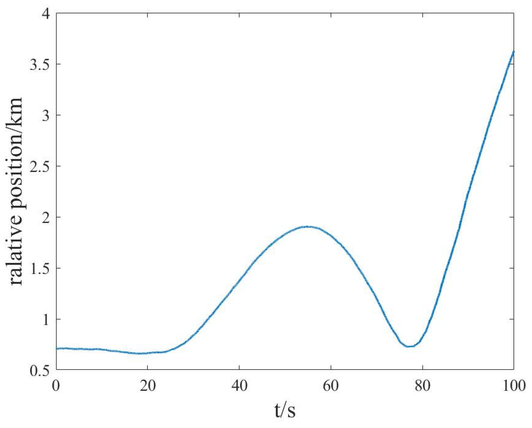
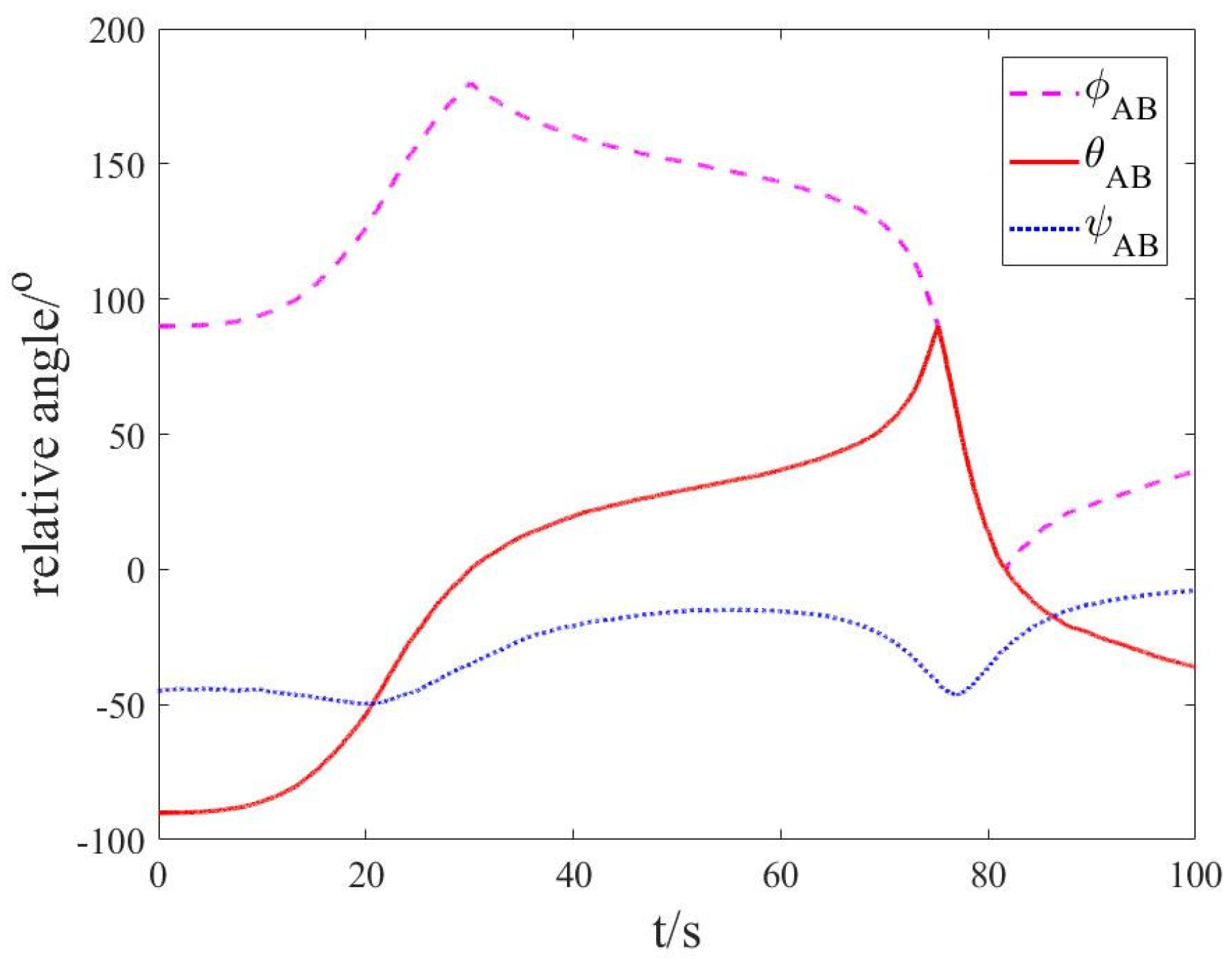
3.1. Simulation Environment and Parameters

The simulation runs in a high-performance computer environment, and its configuration is Intel Xeon Silver 4215R/Tray CPU (main frequency is 3.2 GHz), NVIDIA Geforce Titan RTX professional graphics card, 32G DDR4 RAM, SSD Samsung 480 GB 2.5” SATA hard disk, and Windows 10 operation system with 64-bit. The MATLAB 2019 software is used to realize the real-time simulation result analysis of the proposed method in this paper.

The eight GNSS receivers are equipped on the nose, tail, and two wings of UAV A and UAV B to measure and output the position information in real time. We assume that the initial positions of the nose, tail, left wing, and right wing of UAV A are (0, 1.05, 2) km, (0, 0.93, 2) km, (−0.04, 1, 2) km, and (0.04, 1, 2) km, and the initial positions of the nose, tail, left wing, and right wing of UAV B are (0, 1.55, 2.5) km, (0, 1.43, 2.5) km, (−0.04, 1.5, 2.5) km, and (0.04, 1.5, 2.5) km. The initial positions of the centroids of UAV A and B are (0, 1, 2) km and (0, 1.5, 2.5) km, and their flight motion model is:

$$\{\begin{array}{l}{v}_A=\left[\begin{array}{c}0.35\cos {\displaystyle \frac{t}{16}}+{\delta }_x\\ 0.35\cos {\displaystyle \frac{t}{19}}+{\delta }_y\\ 0.25+0.1*\left({\delta }_z-0.5\right)\end{array}\right]\\ x_A=x_{A0}+v_{A}t\end{array}$$

(33)

where x_A0 is the initial position of the center of mass of UAV A and ${\left({\delta }_x,{\delta }_y,{\delta }_z\right)}^T$ is the random noise.

$$\{\begin{array}{l}{v}_B=\left[\begin{array}{c}0.35\cos {\displaystyle \frac{t}{16.5}}+{\xi }_x\\ 0.35\cos {\displaystyle \frac{t}{18.5}}+{\xi }_y\\ 0.25+0.1*\left({\xi }_z-0.5\right)\end{array}\right]\\ x_B=x_{B0}+v_{B}t\end{array}$$

(34)

where x_B0 is the initial position of the center of mass of UAV B and ${\left({\xi }_x,{\xi }_y,{\xi }_z\right)}^T$ is the random noise.

The formula of the relative position and the angle between UAV A and UAV B can be written as:

$$r_{AB}=\sqrt{{\left(x_{Ax}-x_{Bx}\right)}^2+{\left(x_{Ay}-x_{By}\right)}^2+{\left(x_{Az}-x_{Bz}\right)}^2}$$

(35)

where x_A = (x_Ax, x_Ay, x_Az)^T and x_B = (x_Bx, x_By, x_Bz)^T.

$$\{\begin{array}{l}{\varphi }_{AB}=\arccos {\displaystyle \frac{x_{Ax}-x_{Bx}}{r_{AB}\cos {\psi }_{AB}}}\\ {\theta }_{AB}=\arcsin {\displaystyle \frac{x_{Ay}-x_{By}}{r_{AB}\cos {\psi }_{AB}}}\\ {\psi }_{AB}=\arcsin {\displaystyle \frac{x_{Az}-x_{Bz}}{r_{AB}}}\end{array}$$

(36)

Setting the simulation time as t = 100 s, the flight trajectory, true relative position, and angle of UAV A and UAV B are shown in Figure 2, Figure 3 and Figure 4.

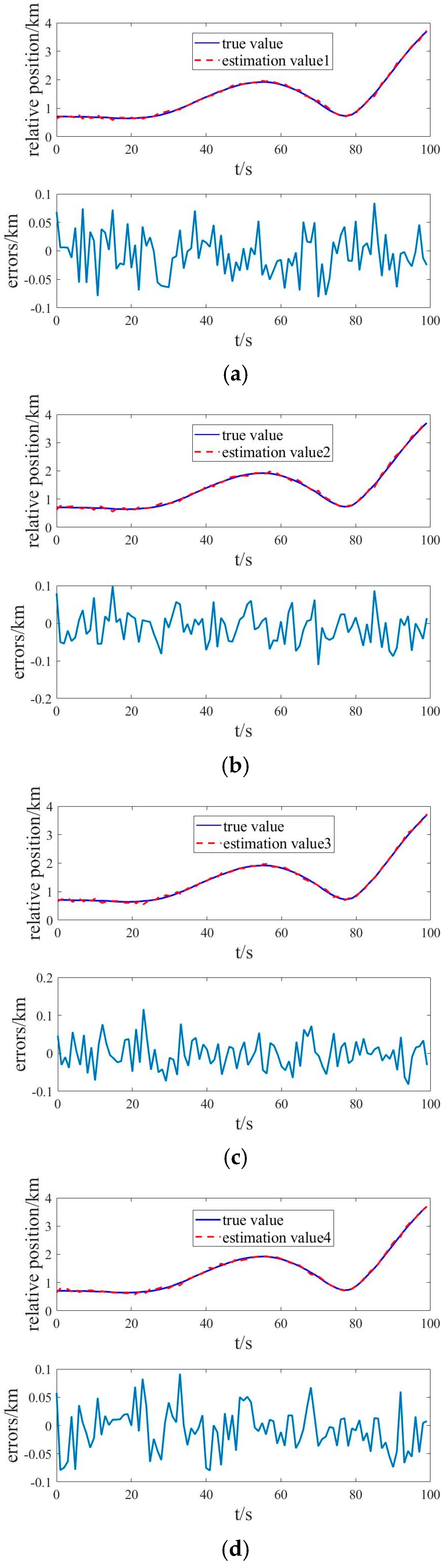
3.2. Simulation Results and Analysis

According to the design scheme of the relative pose estimation in Figure 1, let the measurement points 123 on UAV A determine the equivalent triangle plane as A1, the measurement points 124 on UAV A determine the equivalent triangle plane as A2, the measurement points 134 on UAV A determine the equivalent triangle plane as A3, the measurement points 234 on UAV A determine the equivalent triangle plane as A4, the measurement points 567 on UAV B determine the equivalent triangle plane as B1, the measurement points 568 on UAV B determine the equivalent triangle plane as B2, the measurement points 578 on UAV B determine the equivalent triangle plane as B3, and the measurement points 678 on UAV B determine the equivalent triangle plane as B4. The relative position estimation results and the errors between the estimation results and the true relative position of the equivalent spatial triangle planes A1 and B1, A2 and B2, A3 and B3, and A4 and B4 are shown in Figure 5a–d.

As can be seen from Figure 5, the relative position estimation results of the equivalent triangle planes A1 and B1, A2 and B2, A3 and B3, and A4 and B4 are very close to the true relative position results, and the estimation error is small. In addition, the estimation results between different triangle planes are very similar, which means that the equivalent triangle planes determined by any three points on the UAV can aptly estimate the relative position of the UAVs, and the accuracy of the estimation results is high.

The relative angle estimation result and the errors between the estimation results and the true relative angle of the equivalent spatial triangle planes A1 and B1, A2 and B2, A3 and B3, and A4 and B4 are shown in Figure 6a–d.

As can be seen from Figure 6, the relative angle estimation results of the equivalent triangle planes A1 and B1, A2 and B2, A3 and B3, and A4 and B4 are very close to the true relative angle results, and the estimation error is small. In addition, the estimation results between different triangle planes are very similar, which means that the equivalent triangle planes determined by any three points on the UAV can aptly estimate the relative position of the UAVs, and the accuracy of the estimation results is high.

As can be seen from Figure 5 and Figure 6, the relative pose method based on the equivalent triangle plane can accurately estimate the relative pose of the UAV and has a high estimation accuracy.

We let the equivalent quadrilateral plane of UAV A be A and the equivalent quadrilateral plane of UAV B be B. The relative position estimation results and the errors between the estimation results and the true relative position of the equivalent quadrilateral planes A and B are shown in Figure 7. The relative angle estimation result and the errors between the estimation results and the true relative angle of the equivalent quadrilateral planes A and B are shown in Figure 8.

As can be seen from Figure 7 and Figure 8, the relative pose method based on the equivalent quadrilateral plane can accurately estimate the relative pose of the UAV and has a high estimation accuracy. Compared with the relative pose method based on the equivalent triangle plane, the estimation results and accuracy of the two are very similar, which shows that if the measurement values of the three GNSS receivers on the UAV are known, the relative pose information of the UAV can be aptly estimated.

In the process of receiving data, due to the influence of external factors, the measurement data of the GNSS receivers will produce errors. In this section, the influence of the measurement errors on the estimation results is analyzed as follows. If the measurement data of GNSS receiver 1 has a measurement error, the estimation results of the relative pose of the UAVs are shown in Figure 9. The relative estimation accuracy is shown in

Table 1. Relative estimation accuracy.

Relative Estimation Accuracy	RMSE
	Relative Position/km	φ/°	θ/°	ψ/°
Estimation value 1 and true value	0.028	22.5	2.2	18.9
Estimation value 2 and true value	0.031	25.3	1.9	20.2
Estimation value 3 and true value	0.025	20.8	1.7	22.3
Estimation value 4 and true value	0.009	3.2	2.8	3.1
Estimation value 5 and true value	0.019	15.7	1.3	24.7

.

If the measurement data of GNSS receiver 2 has a measurement error, the estimation results of the relative pose of the UAVs are shown in Figure 10. The relative estimation accuracy is shown in

Table 2. Relative estimation accuracy.

Relative Estimation Accuracy	RMSE
	Relative Position/km	φ/°	θ/°	ψ/°
Estimation value 1 and true value	0.032	31.6	1.5	21.1
Estimation value 2 and true value	0.038	33.1	1.7	22.8
Estimation value 3 and true value	0.010	2.5	0.9	1.1
Estimation value 4 and true value	0.041	30.9	2.1	19.7
Estimation value 5 and true value	0.022	32.2	2.0	18.9

.

As can be seen from Figure 9 and Figure 10 and Table 1 and Table 2, the measurement errors can affect the results of the relative pose estimation, but they will only affect the relative pose estimation results of the equivalent polygonal planes including the measurement points with the measurement errors. Compared with the relative pose method based on the equivalent triangle plane, the relative pose method based on the equivalent quadrilateral plane is less affected by measurement errors, which means that the relative pose estimation method based on the multi-GNSS fusion to determine the equivalent polygon plane has good robustness. In addition, the position of the GNSS receiver with the error can be judged by the influence of the measurement errors on the estimation result.

Based on the above simulation results, it can be seen that the method proposed in this paper can more accurately estimate the relative pose results of the UAVs and can effectively identify the position of the GNSS receiver with measurement errors; at the same time, it also shows that the relative pose estimation method based on multi-data fusion used to determine the equivalent spatial plane has good robustness.

4. Conclusions

In this paper, we propose a relative pose estimation method for UAVs based on the equivalent spatial plane. In terms of theoretical derivation, four GNSS receivers are installed on the UAV to measure and output the position information, and three different GNSS measurement values are selected to calculate the normal vector and determine the equivalent triangle plane equation. The objective function based on the minimum sum of the squares of distances from the four points to the spatial plane is established, and the Gauss–Newton iteration method is used to iteratively calculate the normal vector and solve the equivalent quadrilateral plane equation. When the equivalent polygonal plane equation of the UAVs and the GNSS measurement values are known, the relative position and angle between the UAVs are calculated. Finally, the influence of the measurement errors in the measurement data on the estimation results of the relative pose is analyzed. In terms of the simulation analysis, the simulation environment and initial parameters are conducted to verify the performance of the proposed method.

The simulation results show that the proposed method can accurately estimate the relative attitude of the tanker/receiver without relying on precise mathematical models; the measurement errors only affect the relative pose estimation results including the measurement points with measurement errors, which show that the proposed method can achieve the detection and diagnosis of abnormal changes in GNSS data. The simulation results verify the applicability and effectiveness of the proposed method in this paper, and the research results can provide a certain theoretical and practical basis for cluster control and autonomous formation.

References

1. Xu, X.B.; Duan, H.B.; Guo, Y.J.; Deng, Y.M. A cascade adaboost and CNN algorithm for drogue detection in UAV autonomous aerial refueling. Neurocomputing 2020, 408, 121–134. [Google Scholar] [CrossRef]
2. Chao, Z.; Zhou, S.L.; Ming, L.; Zhang, W.G.; Scalia, M. UAV Formation Flight Based on Nonlinear Model Predictive Control. Math. Probl. Eng. 2012, 2012, 181–188. [Google Scholar] [CrossRef]
3. de Marina, H.G.; Espinosa, F.; Santos, C. Adaptive UAV Attitude Estimation Employing Unscented Kalman Filter, FOAM and Low-Cost MEMS Sensors. Sensors 2012, 12, 9566–9585. [Google Scholar] [CrossRef] [PubMed]
4. Li, J. Relative pose measurement of binocular vision based on feature circle. Optik 2019, 194, 163121. [Google Scholar] [CrossRef]
5. Williamson, W.R.; Glenn, G.J.; Dang, V.T.; Speyer, J.L.; Stecko, S.M.; Takacs, J.M. Sensor fusion applied to autonomous aerial refueling. J. Guid. Control Dyn. 2009, 32, 262–275. [Google Scholar] [CrossRef]
6. Gross, J.; Gu, Y.; Rhudy, M.; Chahl, J. Fixed-Wing UAV Attitude Estimation Using Single Antenna GPS Signal Strength Measurements. Aerospatial 2016, 3, 14. [Google Scholar] [CrossRef]
7. Korbly, R. Sensing Relative Attitudes for Automatic Docking. J. Guid. Control Dyn. 1983, 6, 213–215. [Google Scholar] [CrossRef]
8. Koksal, N.; Jalalmaab, M.; Fidan, B. Adaptive Linear Quadratic Attitude Tracking Control of a Quadrotor UAV Based on IMU Sensor Data Fusion. Sensors 2018, 19, 46. [Google Scholar] [CrossRef] [PubMed]
9. Li, B.R.; Mu, C.D.; Wu, B.T. Vision based close-range relative pose estimation for autonomous aerial refueling. J. Tsinghua Univ. (Sci. Technol.) 2012, 52, 1664–1669. [Google Scholar] [CrossRef]
10. Campa, G.; Napolitano, M.; Fravolini, M. Simulation environment for machine vision based aerial refueling for UAVs. IEEE Trans. Aerosp. Electron. Syst. 2009, 45, 138–151. [Google Scholar] [CrossRef]
11. Mammarella, M.; Campa, G.; Napolitano, M.R.; Fravolini, M.L. Comparison of point matching algorithms for the UAV aerial refueling problem. Mach. Vis. Appl. 2010, 21, 241–251. [Google Scholar] [CrossRef]
12. Fravolini, M.L.; Campa, G.; Napolitano, M.R. Evaluation of machine vision algorithms for autonomous aerial refueling for unmanned aerial vehicles. J. Aerosp. Comput. Inf. Commun. 2007, 4, 968–985. [Google Scholar] [CrossRef]
13. Ding, M.; Wei, L.; Wang, B. Vision-based estimation of relative pose in autonomous aerial refueling. Chin. J. Aeronaut. 2011, 6, 807–815. [Google Scholar] [CrossRef]
14. Doebbler, J.; Spaeth, T.; Valasek, J.; Monda, M.J.; Schaub, H. Boom and receptacle autonomous air refueling using visual snake optical sensor. J. Guid. Control Dyn. 2009, 30, 175–1769. [Google Scholar] [CrossRef]
15. Zhang, L.M.; Zhu, F.; Hao, Y.M.; Pan, W. Optimization-based non-cooperative spatialcraft pose estimation using stereo cameras during proximity operations. Appl. Opt. 2017, 56, 4522–4531. [Google Scholar] [CrossRef] [PubMed]
16. Zhang, L.M.; Zhu, F.; Hao, Y.M.; Pan, W. Rectangular-structure-based pose estimation method for non-cooperative rendezvous. Appl. Opt. 2018, 57, 6164–6173. [Google Scholar] [CrossRef] [PubMed]
17. Hinterstoisser, S.; Lepetit, V.; Ilic, S.; Holzer, S.; Konolige, K.; Bradski, G.; Navab, N. Technical Demonstration on Model Based Training, Detection and Pose Estimation of Texture-Less 3D Objects in Heavily Cluttered Scenes. In Proceedings of the 12th European Conference on Computer Vision (ECCV), Florence, Italy, 7–13 October 2012; Volume 7585, pp. 593–596. [Google Scholar] [CrossRef]
18. Weaver, A.D.; Veth, M.J. Image-based relative navigation for the autonomous refueling problem using predictive rendering. In Proceedings of the 2009 IEEE Aerospace Conference, Big Sky, MT, USA, 7–14 March 2009; IEEE Computer Society: Piscataway, NJ, USA, 2009; pp. 1–13. [Google Scholar] [CrossRef]
19. Li, G. Three-Dimensional Attitude Measurement of Complex Rigid Flying Target Based on Perspective Projection Matching. Ph.D. Thesis, Harbin Institute of Technology, Harbin, China, 2015. Available online: https://kns.cnki.net/KCMS/detail/detail.aspx?dbname=CMFD201601&filename=1015980350.nh (accessed on 1 July 2015).
20. Liebelt, J.; Schmid, C.; Schertler, K. Viewpoint-independent object class detection using 3D feature maps. In Proceedings of the 2008 IEEE Computer Society Conference on Computer Vision and Pattern Recognition (CVPR 2008), Anchorage, AK, USA, 23–28 June 2008; pp. 978–986. [Google Scholar] [CrossRef]
21. Teng, X.C.; Yu, Q.F.; Luo, J.; Zhang, X.H.; Wang, G. Pose Estimation for Straight Wing Aircraft Based on Consistent Line Clustering and Planes Intersection. Sensors 2019, 19, 342. [Google Scholar] [CrossRef] [PubMed]
22. Williamson, W.R.; Abdel-Hafez, M.F.; Rhee, I.; Song, E.J.; Wolfe, J.D.; Chichka, D.F.; Speyer, J.L. An instrumentation system applied to formation flight. IEEE Trans. Control Syst. Technol. 2007, 15, 75–85. [Google Scholar] [CrossRef]
23. Yuan, H.; Xiao, C.; Xiu, S.; Wen, Y.; Zhou, C.; Li, Q. A New Combined Vision Technique for Micro Aerial Vehicle Pose Estimation. Robotics 2017, 6, 6. [Google Scholar] [CrossRef]
24. Strohmeier, M.; Montenegro, S. Coupled GPS/MEMS IMU Attitude Determination of Small UAVs with COTS. Electronics 2017, 6, 15. [Google Scholar] [CrossRef]
25. Eling, C.; Klingbeil, L.; Kuhlmann, H. Real-Time Single-Frequency GPS/MEMS-IMU Attitude Determination of Lightweight UAVs. Sensors 2015, 15, 26212–26235. [Google Scholar] [CrossRef] [PubMed]
26. Fosbury, A.M.; Crassidis, J.L. Relative navigation of air vehicles. J. Guid. Control Dyn. 2008, 31, 824–834. [Google Scholar] [CrossRef]
27. Shao, W.; Chang, X.H.; Cui, P.Y.; Cui, H.T. Coupled feature matching and INS for small body landing navigation. J. Astronaut. 2010, 31, 1748–1755. [Google Scholar] [CrossRef]
28. Wang, L.; Dong, X.M.; Zhang, Z.L. Relative pose measurement based on tightly-coupled INS/Vision. J. Chin. Inert. Technol. 2011, 19, 686–691. [Google Scholar] [CrossRef]
Figure 1. Scheme of relative pose estimation between UAVs.
Drones 08 00383 g001
Figure 2. Flight trajectory of UAVs.
Drones 08 00383 g002
Figure 3. Relative position.
Drones 08 00383 g003
Figure 4. Relative angle.
Drones 08 00383 g004
Figure 5. Relative position estimation and errors. (a) Relative position estimation and error between true value and estimation value 1; (b) Relative position estimation and error between true value and estimation value 2; (c) Relative position estimation and error between true value and estimation value 3; (d) Relative position estimation and error between true value and estimation value 4.
Drones 08 00383 g005
Figure 6. Relative angle estimation and errors. (a) Relative angles estimation and error between true value and estimation value 1; (b) Relative angles estimation and error between true value and estimation value 2; (c) Relative angles estimation and error between true value and estimation value 3; (d) Relative angles estimation and error between true value and estimation value 4.
Drones 08 00383 g006
Figure 7. Relative position estimation and errors.
Drones 08 00383 g007
Figure 8. Relative angle estimation and errors.
Drones 08 00383 g008
Figure 9. Relative pose estimation results.
Drones 08 00383 g009
Figure 10. Relative pose estimation results.
Drones 08 00383 g010