Enhanced Trajectory Forecasting for Hypersonic Glide Vehicle via Physics-Embedded Neural ODE

Abstract

Forecasting hypersonic glide vehicle (HGV) trajectories accurately is crucial for defense, but traditional methods face challenges due to the scarce real-world data and the intricate dynamics of these vehicles. Data-driven approaches based on deep learning, while having emerged in recent years, often exhibit limitations in predictive accuracy and long-term forecasting. Whereas, physics-informed neural networks (PINNs) offer a solution by incorporating physical laws, but they treat these laws as constraints rather than fully integrating them into the learning process. This paper presents PhysNODE, a novel physics-embedded neural ODE model for the precise forecasting of HGV trajectories, which directly integrates the equations of HGV motion into a neural ODE. PhysNODE leverages a neural network to estimate the hidden aerodynamic parameters within these equations. These parameters are then combined with observable physical quantities to form a derivative function, which is fed into an ODE solver to predict the future trajectory. Comprehensive experiments using simulated datasets of HGV trajectories demonstrate that PhysNODE outperforms the state-of-the-art data-driven and physics-informed methods, particularly when training data is limited. The results highlight the benefit of embedding the physics of the HGV motion into the neural ODE for improved accuracy and stability in trajectory predicting.

1. Introduction

Hypersonic glide vehicle (HGV), with its ability to maneuver at extreme speeds, presents a significant challenge to modern air defense systems [1]. Accurate trajectory forecasting is essential for effective interception, enabling the development of robust defense strategies, timely responses, and the protection of critical infrastructure [2]. However, predicting glide trajectories is very difficult due to the vehicles’ high velocity, complex maneuvering patterns, and the potential scarcity of real-world training data [3].

Traditional methods for predicting HGV trajectories typically include analytical methods, which derive closed-form solutions; numerical integration methods, which iteratively solve the equations of motion; and function approximation methods, which fit simplified models to the observed data [4]. However, these methods often perform poorly in accurately predicting glide trajectories for extended periods, due to the complexities of the flight dynamics.

While data-driven methods employing deep learning networks such as LSTM [5], CNN [6,7], and Transformers [8] have shown promise in handling long-term prediction, their reliance on large training datasets presents a notable limitation in scenarios where obtaining sufficient data is difficult [9]. Given that the glide phase of an HGV is unpowered, meaning its motion is governed entirely by aerodynamic forces and gravitational interactions, adhering strictly to the fundamental laws of physics. Therefore, incorporating inherent physical knowledge into the prediction model holds potential for enhancing the trajectory prediction accuracy, warranting further research.

To address the shortcomings of purely data-driven methods, physics-informed neural networks (PINNs) offer an effective approach by intergrating physical laws directly into the training process [10,11]. By leveraging physical laws, PINNs can enhance predictive accuracy while ensuring adherence to the underlying physical principles governing the system’s behavior, which is crucial for reliable trajectory forecasting. Moreover, PINNs can achieve high performance with smaller datasets due to the embedded physical knowledge supplementing data-driven learning, enhancing generalization capability, making them particularly well-suited for real-world applications where data collection is often limited [12,13].

However, despite these advantages, PINNs also have limitations. They typically treat physical laws as constraints added as penalty terms in the loss function during training [14]. This passive incorporation can lead to several issues, for one thing, incorporating physical constraints into the loss function requires careful tuning of multiple balancing factors, which can be complex. For another, this approach does not fully exploit the guiding power of physical laws during the learning process, potentially leading to suboptimal predictions and poor generalization to unseen data.

To overcome the limitations of conventional PINNs, particularly the challenges of data scarcity and the highly nonlinear dynamics of the HGV flight, this paper introduces Physics-embedded Neural ODE (PhysNODE), a novel physics-embedded neural ODE model. Unlike traditional PINNs, PhysNODE directly integrates the HGV motion equations into the model architecture. This approach ensures more accurate trajectory predictions by actively guiding the learning process with both physical principles and data patterns.

PhysNODE decomposes the flight dynamics equations into observable and predictable components. A neural network predicts the unobservable aerodynamic parameters, which are then encapsulated within an ODE block. This ODE block is subsequently incorporated into a neural ODE framework [15], enabling the model to predict the HGV trajectory sequence based on the aerodynamic principles. To facilitate efficient training, a adjoint state method is employed for gradient computation.

This work contributes in three key aspects:

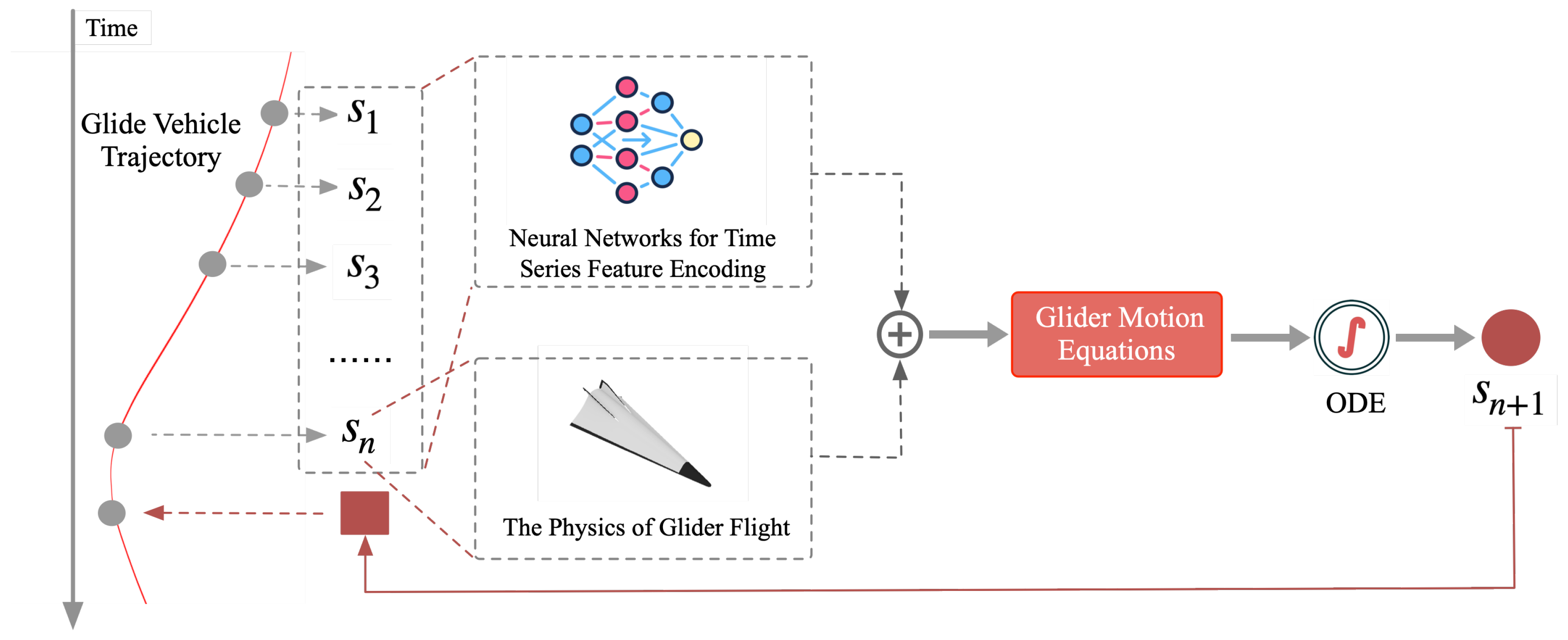
• We propose PhysNODE, a novel physics-embedded neural ODE framework that integrates physical knowledge directly into the model architecture for improved the HGV trajectory prediction.
• We demonstrate the effectiveness of PhysNODE through extensive experiments, showcasing its enhanced performance compared to the state-of-the-art data-driven and physics-informed methods, particularly on small datasets.
• We provide a detailed analysis of how physics integration influences the model, focusing on its impact on prediction accuracy, stability, and generalization ability.

The rest of this paper is organized as follows: Section 2 provides a comprehensive review of related work in the HGV trajectory prediction, covering both data-driven and physics-informed approaches. Section 3 presents the necessary background information, including the governing equations of motion for HGVs, a formal definition of the trajectory prediction problem, and an overview of Neural ODEs. Section 4 details the methodology of our proposed PhysNODE model, including its architecture, the integration of physical knowledge, and the training procedure. Section 5 describes the construction of the simulated HGV trajectory datasets used in our experiments. Section 6 presents the experimental results and provides an in-depth analysis, comparing the performance of PhysNODE with state-of-the-art methods. Finally, Section 7 concludes the paper, summarizing the key findings and discussing potential future research directions.

2. Related Work

Predicting HGV trajectories is a complex task due to its complex dynamics and high speeds. Recent years have seen significant growth in research utilizing deep learning to tackle this challenge, producing several noteworthy approaches.

2.1. Data-Driven Approaches

Numerous studies have explored the direct application of deep learning architectures for the prediction of trajectories [16]. Zhang et al. [17] achieved encouraging results using a deep learning model for the motion state recognition and prediction of HGV. Similarly, Xie et al. [18] introduced a dual-channel bidirectional neural network specifically designed for the HGV trajectory prediction. Sun et al. [5] presented an LSTM-based pipeline approach for the trajectory prediction to intercept HGVs. However, these purely data-driven methods often rely on extensive training datasets and may face difficulty in effectively generalizing to unseen scenarios, making them less robust in practical situations where comprehensive datasets are often unavailable.

2.2. Hybrid Approaches

Recognizing the deficiencies of purely data-driven methods, researchers have explored integrating domain knowledge into the forecasting process. For instance, Liu et al. [19] proposes a real-time trajectory prediction method that utilizes a 3D flight corridor constrained by the quasi-equilibrium glide condition. This approach simplifies the prediction problem by employing a reduced-order system of differential equations solved with a semi-analytical algorithm, achieving high prediction speeds suitable for real-time applications. Similarly, Li et al. [20] leverages intention inference to enhance the trajectory prediction by modeling the significance of the strategic locations and inferring the target’s intent. This method improves the forecast accuracy, especially for the long-term predictions.

2.3. Integrating Physical Laws into Neural Networks

Researchers also have sought to directly embed laws of physics into deep neural networks, forming physics-informed deep learning models [21]. This integration aims to leverage the strengths of both data-driven learning and physics-based modeling, enabling more accurate, physically consistent, and generalizable predictions. For instance, Djeumou et al. [11] proposed physics-informed neural networks for dynamical systems modeling, embedding physical laws within the learning process. Ren et al. [10] developed a physics-informed Transformer for the long-term HGV trajectory prediction, demonstrating the potential of integrating physics knowledge into transformer architectures. However, effectively encoding and integrating complex physical laws into these models, especially considering the highly nonlinear dynamics of the HGV flight, remains a significant challenge.

2.4. Neural ODEs for Trajectory Prediction

Neural ODEs [15] present a powerful tool for modeling continuous-time dynamical systems, demonstrating potential as an effective tool for the trajectory prediction [22]. By parameterizing the derivative of the system state using a neural network, Neural ODEs can learn the underlying differential equations governing the system’s evolution [23]. This approach allows for flexible handling of irregular time steps and provides a continuous-time representation of the trajectory, resulting in more accurate predictions. However, similar to the difficult encountered with physics-informed deep learning, effectively representing complex physical constraints, such as those governing HGV aerodynamics, within the Neural ODE framework is a crucial aspect that requires further investigation.

3. Background

This section introduces the background for forecasting HGV trajectories. It begins by presenting the governing equations of motion for reentry gliders, followed by a formal definition of the trajectory prediction problem addressed in this work, and an overview of Neural ODEs, which serve as the foundation for our model.

3.1. Motion Equations

An HGV is typically launched by a rocket that carries it to near space, usually to an altitude below 80 km. Upon reaching the desired altitude and velocity, the glider is released from the launch vehicle and begins its unpowered glide phase. During this phase, the HGV uses aerodynamic lift generated at hypersonic speeds (generally Mach 5 and above) to maneuver and maintain altitude. A key characteristic of the glider is the formation of a strong shockwave ahead of the vehicle due to extreme air compression. The HGV is designed to exploit this shockwave, using the lift generated by its interaction with the vehicle’s body and minimizing aerodynamic drag to achieve long-range, rapid strikes. As the glide phase of the HGV is governed by physical laws, its trajectory can be predicted by utilizing these laws to model its motion.

The motion of an HGV during its glide phase is governed by a set of three-degree-of-freedom equations. Neglecting the influence of Earth’s rotation, these equations can be represented as follows [24]:

$$\left\{\begin{array}{cc}\hfill {\displaystyle \frac{dh}{dt}}& =v\mathit{sin}\gamma \hfill \\ \hfill {\displaystyle \frac{d\lambda }{dt}}& ={\displaystyle \frac{v\mathit{cos}\gamma \mathit{sin}\psi }{r\mathit{cos}\varphi }}\hfill \\ \hfill {\displaystyle \frac{d\varphi }{dt}}& ={\displaystyle \frac{v\mathit{cos}\gamma \mathit{cos}\psi }{r}}\hfill \\ \hfill {\displaystyle \frac{dv}{dt}}& =-g\mathit{sin}\gamma -{\displaystyle \frac{D}{m}}\hfill \\ \hfill {\displaystyle \frac{d\gamma }{dt}}& =-{\displaystyle \frac{g}{v}}\mathit{cos}\gamma +{\displaystyle \frac{v}{r}}\mathit{cos}\gamma +{\displaystyle \frac{L\mathit{cos}\sigma }{mv}}\hfill \\ \hfill {\displaystyle \frac{d\psi }{dt}}& ={\displaystyle \frac{v}{r}}\mathit{cos}\gamma \mathit{sin}\psi \mathit{tan}\varphi +{\displaystyle \frac{L\mathit{sin}\sigma }{mv\mathit{cos}\gamma }}\hfill \end{array}\right.$$

(1)

Let h denote the altitude of a HGV, v represent the glider’s velocity relative to the Earth, $\lambda$ and $\varphi$ correspond to the longitude and latitude of the glider’s current position, respectively. Additionally, let $\gamma$ signify the flight path angle, $\psi$ represent the heading angle, and $\sigma$ denote the bank angle. The mass of a HGV is denoted by m, and r represents the radial distance from the HGV to the Earth’s center. The relationship between the altitude h and the radial distance r is given by:

$$r=h+R_{\oplus }$$

(2)

where $R_{\oplus }$ is the Earth’s radius, which is approximately 6371.20392 km.

The aerodynamic forces, lift (L) and drag (D), are critical components of these equations and are calculated using the following standard aerodynamic formulas:

$$L={\displaystyle \frac{1}{2}}\rho V^{2}S{C}_{L}D={\displaystyle \frac{1}{2}}\rho V^{2}S{C}_D$$

(3)

where $\rho$ is the atmospheric density, S is the reference area of the HGV, and $C_L$ and $C_D$ are the lift and drag coefficients, respectively. These coefficients are functions of the angle of attack $\alpha$ and Mach number $M_{\alpha }$, and are typically obtained from aerodynamic interpolation tables or fitted functions. The Mach number is defined as the ratio of the HGV velocity to the speed of sound $V_s$.

The HGV possess sophisticated maneuvering capabilities, enabling them to execute complex flight paths through adjustments in both longitudinal and lateral directions. Longitudinal maneuvers involve transitions between balanced glide and skip-glide states. In balanced glide, the HGV maintains equilibrium by adjusting its bank angle to balance gravitational and lift forces, resulting in a near-constant flight path angle and minimal angle of attack. When conditions for balanced glide are not met, the HGV enters a skip-glide state, characterized by periodic oscillations in altitude and flight path angle. The angle of attack in skip-glide is often represented by simplified functions, such as constant values, piecewise linear functions, or linear functions. Lateral maneuvering is achieved through the adjustment of the roll angle or the bank angle, allowing the HGV to execute turns, including complex maneuvers like C-shaped or S-shaped flight paths [1].

This study focuses on two complex trajectory patterns: skip-glide with lateral C-shaped and S-shaped maneuvers (Figure 1). These maneuvers, which have significant practical relevance, enhance target accuracy and survivability by dissipating excess energy to prevent overshoot and aiding in evading interception.

3.2. Problem Description

Let a single HGV trajectory be represented as a time series of state vectors:

$$\{{\mathbf{s}}_{obs\left(1\right)},{\mathbf{s}}_{obs\left(2\right)},...,{\mathbf{s}}_{obs\left(N\right)}\}$$

(4)

where ${\mathbf{s}}_{obs\left(t\right)}\in {\mathbb{R}}^d$ represents the observable state vector at time step t, containing d variables as follows:

$$s_{obs\left(t\right)}={[h\left(t\right),\lambda \left(t\right),\varphi \left(t\right),v\left(t\right),\gamma \left(t\right),\psi \left(t\right)]}^{\mathrm{T}}$$

(5)

where the flight path angle $\gamma \left(t\right)$ can be derived using central differencing from velocity measurements and other parameters can be observed directly.

We use a sliding window of size P to define the observation window and a prediction horizon of F to define the target trajectory to be predicted. This results in a set of input-output pairs $(T_j,{\widehat{T}}_j)$, generated as follows:

$$T_j=\{{\mathbf{s}}_{obs\left(j\right)},{\mathbf{s}}_{obs(j+1)},...,{\mathbf{s}}_{obs(j+P-1)}\}$$

(6)

$${\widehat{T}}_j=\{{\mathbf{s}}_{obs(j+P)},{\mathbf{s}}_{obs(j+P+1)},...,{\mathbf{s}}_{obs(j+P+F-1)}\}$$

(7)

where $1\le j\le N-P-F+1$. Each $T_j\in {\mathbb{R}}^{P\times d}$ represents a sequence of P consecutive state vectors, serving as the input to the model. Each ${\widehat{T}}_j\in {\mathbb{R}}^{F\times d}$ represents the corresponding F future state vectors, forming the target trajectory to be predicted.

3.3. Neural ODEs

This study is based on Neural ODEs. Unlike traditional neural networks that process time series as discrete time steps, Neural ODEs embrace a continuous-time perspective, utilizing neural networks to learn the differential equations governing the evolution of trajectories. PhysNODE extends this paradigm by incorporating physics-based calculations directly into the neural network, ensuring the physical consistency of the learned dynamics. Specifically, consider the system state represented as $s\left(t\right)$ at time t. A neural network models the rate of change of this state over time. The system dynamics can be expressed by the following differential equation:

$${\displaystyle \frac{ds\left(t\right)}{dt}}=f(s\left(t\right),t,\theta )$$

(8)

where $\theta$ is the parameters of the neural network. Given an initial state $s\left(t_0\right)$, an ODE solver can be used to solve this equation and predict the state $s\left(t_0\right)$ at any future time point.

Training Neural ODEs involves optimizing parameters $\theta$ to minimize the discrepancy between predicted and actual trajectories. This requires computing the gradient of a loss function $L\left(·\right)$ with respect to $\theta$. A common approach involves defining the loss based on the final state $s\left(t_1\right)$:

$$L\left(s\left(t_1\right)\right)=L\left(s\left(t_0\right)+{\int }_{t_0}^{t_1}f(s\left(t\right),t,\theta )dt\right)=L\left(ODESolver(s\left(t_0\right),f,t_0,t_1,\theta )\right)$$

(9)

Directly applying traditional backpropagation to compute this gradient would necessitate storing all intermediate states from the forward propagation through the ODE solver. This is a major issue, as the solver often requires numerous steps, leading to potential memory explosion, especially for complex ODEs solved with high precision. To address this, Neural ODEs employ the adjoint sensitivity method, which efficiently computes gradients by solving an auxiliary ODE backward in time, avoiding the need to store all intermediate states. (See Chen et al. [15] for a detailed explanation of this method).

4. The PhysNODE Model

This section details the methodology of PhysNODE, our novel framework for the HGV trajectory prediction. First, we present the principles of our method. Then, we delve into the core components of PhysNODE, including the physics-embedded network for integrating physical knowledge, and the specific neural network architecture. Finally, we outline the algorithm workflow.

4.1. Model Formulation

For the intercepting party, it is typically difficult to accurately predict the trajectory of an HGV during its glide phase due to the unavailability of aerodynamic parameters such as lift and drag coefficients, mass, and reference area. To address this, we propose PhysNODE, a physics-embedded neural ODE model (Figure 2) that integrates data-driven learning with the aerodynamic parameters governing HGV motion.

As shown in Figure 2, PhysNODE is comprised of two primary components: a neural network and a physics-based model. These two components operate in parallel. A series of observed states $\mathbf{s}$ are fed into the neural network for time-series encoding, predicting the unknown aerodynamic parameters. Simultaneously, the last observed state $s_n$ is input into the physics module, which computes the time derivatives of the observable state variables (as shown in Equation (14) in the following subsection). The outputs from the neural network and the physics module form a complete HGV motion equation (as shown in Equation (1)). Using an ODE solver, the next state $s_{n+1}$ can be determined, and this process is recursively applied to predict the trajectory over a time range.

This process can be expressed as follows:

$$\begin{array}{cc}\hfill {\widehat{s}}_{n+1}& =\mathrm{NN}([s_1,s_2,\cdots ,s_n];{\theta }_{nn})+\mathrm{Phys}(s_n;{\theta }_{phys})\hfill \\ \hfill s_{n+1}& =\mathrm{ODESolver}\left({\widehat{s}}_{n+1}\right)\hfill \end{array}$$

(10)

where NN represents the neural network component, Phys represents the physics-based model that incorporates the physical laws for the motion of the glide vehicle, and ${\theta }_{·}$ is the parametrics for each component. The ODESolver module derives the next state $s_{n+1}$ by integrating the state differential ${\widehat{s}}_{n+1}$ based on the physical motion equations (Equation (1)).

In contrast, the PINN model predicts as follows:

$$\begin{array}{cc}\hfill & s_{n+1}=\mathrm{NN}([s_1,s_2,\cdots ,s_n];{\theta }_{nn})\hfill \\ \hfill & \mathrm{s}.\mathrm{t}.\mathcal{L}(f\left(s_{n+1}\right);{\theta }_{phy{s}_1,phy{s}_2,\cdots ,phy{s}_n})\hfill \end{array}$$

(11)

where $\mathcal{L}$ represents the constraint conditions, and $phy{s}_n$ represents a physical constraint.

As shown in Equation (11), PINN treats physical information as a constraint, requiring balancing factors between different physical constraint terms, which can be challenging for model tuning. On the other hand, our method incorporates physical information directly into the forecasting process, avoiding this issue.

Overall, PhysNODE combines the predictive power of neural networks with the adherence to physical laws of physics-based models, providing a robust framework for accurately predicting HGV trajectories despite uncertainties in aerodynamic parameters. This innovative approach ensures that the model not only learns from data but also respects the fundamental physical principles governing HGV motion.

4.2. Physics-Embedded Network

The core mechanism of PhysNODE lies in integrating prior physical knowledge. To this end, PhysNODE first decomposes the variables within the HGV motion equations (Equation (1)) into observable and predicted components. The observable component $s_{obs\left(t\right)}$ have been discriped as Equation (5). The predicted component represents the aerodynamic parameters, which are important for accurate trajectory prediction but cannot be directly measured or inferred at time t:

$$p\left(t\right)={[{\displaystyle \frac{D\left(t\right)}{m}},{\displaystyle \frac{Lcos\left(\sigma \right(t\left)\right)}{m}},{\displaystyle \frac{Lsin\left(\sigma \right(t\left)\right)}{m}}]}^{\mathrm{T}}$$

(12)

By integrating the observable and predicted quantities, PhysNODE forms a comprehensive state derivative vector, which encapsulates the complete dynamics of a HGV. First, PhysNODE calculates the time derivatives of the observable state variables:

$${\displaystyle \frac{d{s}_{obs\left(t\right)}}{dt}}=f_{phy}(s_{obs\left(t\right)},t)$$

(13)

where $f_{phy}$ represents the physics-based function that maps the observable state vector to its derivative, which is derived from the HGV motion equations as follows:

$$\left\{\begin{array}{c}\begin{array}{cc}\hfill {\displaystyle \frac{dh}{dt}}& =vsin\gamma \hfill \\ \hfill {\displaystyle \frac{d\lambda }{dt}}& ={\displaystyle \frac{vcos\gamma sin\psi }{rcos\varphi }}\hfill \\ \hfill {\displaystyle \frac{d\varphi }{dt}}& ={\displaystyle \frac{vcos\gamma cos\psi }{r}}\hfill \\ \hfill {\displaystyle \frac{dv}{dt}}& =-gsin\gamma \hfill \\ \hfill {\displaystyle \frac{d\gamma }{dt}}& =cos\gamma \left({\displaystyle \frac{v}{r}}-{\displaystyle \frac{g}{v}}\right)\hfill \\ \hfill {\displaystyle \frac{d\psi }{dt}}& ={\displaystyle \frac{vcos\gamma sin\psi tan\left(\varphi \right)}{r}}\hfill \end{array}\hfill \end{array}\right.$$

(14)

Note that the expressions for ${\displaystyle \frac{dv}{dt}},{\displaystyle \frac{d\gamma }{dt}}$, and ${\displaystyle \frac{d\psi }{dt}}$ are incomplete compared to the complete HGV motion equations (Equation (1)), as they do not include the contributions from the unobservable aerodynamic parameters D, $Lcos\left(\sigma \right(t\left)\right)$, $Lsin\left(\sigma \right(t\left)\right)$ and m, respectively. These unobservable parameters, forming the vector $p\left(t\right)$, are predicted by a neural network module as follows:

$$p\left(t\right)=\mathrm{NN}([s_{obs\left(1\right)},s_{obs\left(2\right)},\cdots ,s_{obs\left(t\right)}],t,\theta )$$

(15)

The neural network NN combines CNN and MLP as detailed in Section 4.3. To predict the HGV trajectory, ${\displaystyle \frac{d{s}_{\mathrm{obs}\left(t\right)}}{dt}}$ and $p\left(t\right)$ need to be combined to form the complete state derivative vector, denoted as ${\displaystyle \frac{ds\left(t\right)}{dt}}$:

$${\displaystyle \frac{ds\left(t\right)}{dt}}=f_{phy}(s_{obs\left(t\right)},t)+G·\mathrm{NN}([s_{obs\left(1\right)},s_{obs\left(2\right)},\cdots ,s_{obs\left(t\right)}],t,\theta )$$

(16)

G is a matrix that maps the predicted aerodynamic parameters to their corresponding terms within the HGV motion equations, producing a physically realistic predicted state derivative ${\displaystyle \frac{ds\left(t\right)}{dt}}$ that encompasses all variables required for the complete motion equations (Equation (1)). Following the HGV motion equations, the mapping matrix G is defined as:

$$G=\left[\begin{array}{ccc}0& 0& 0\\ 0& 0& 0\\ 0& 0& 0\\ -1& 0& 0\\ 0& 1/v\left(t\right)& 0\\ 0& 0& 1/\left(v\right(t)\ast cos(\gamma \left(t\right)\left)\right)\end{array}\right]$$

(17)

This complete predicted state derivative ${\displaystyle \frac{ds\left(t\right)}{dt}}$, now encompassing both the physically derived and neural network predicted components, is formulated as an ODE block and passed to an ODE solver (e.g., ode45) for numerical integration. This process generates the predicted HGV trajectory by solving the following equation:

$$s(t+f)=\mathrm{ODESolver}({\displaystyle \frac{ds\left(t\right)}{dt}},t,t+f,\theta )$$

(18)

where t and $t_f$ are the start and end times respectively.

4.3. Neural Network Architecture

As shown in Figure 3, the PhysNODE framework designs a hybrid neural network architecture that integrates 1D Convolutional Neural Networks (1D CNN) [7] with Multi-Layer Perceptrons (MLP), aiming to accurately estimate the key aerodynamic parameters $p\left(t\right)$.

Each 1D CNN layer is configured with a unique kernel size, acting as a sliding window on the input time series. Smaller kernels can effectively capture rapid fluctuations and short-term trends in the data, while larger kernels can reveal long-term dependencies and overall trajectory patterns. Mathematically, this process can be expressed as:

$$h_i\left[j\right]=\mathrm{RELU}\left(\sum _{m=1}^M{W}_i\left[m\right]·X[j+m-1]+b_i\right)$$

(19)

where $h_i\left[j\right]$ is the output of the i-th convolution kernel at position j, $W_i\left[m\right]$ is the weight of the i-th kernel, $X[j+m-1]$ is the input value at position $j+m-1$, $b_i$ is the bias of the i-th kernel, and RELU is the activation function defined as $\mathrm{RELU}\left(z\right)=max(0,z)$.

PhysNODE utilizes a three-layer 1D CNN, each layer applying convolution operations as follows:

$$h_i^{\left(1\right)}\left[j\right]=\mathrm{RELU}\left(\sum _{m=1}^{M_1}{W}_i^{\left(1\right)}\left[m\right]·X[j+m-1]+b_i^{\left(1\right)}\right)$$

(20)

$$h_i^{\left(2\right)}\left[j\right]=\mathrm{RELU}\left(\sum _{m=1}^{M_2}{W}_i^{\left(2\right)}\left[m\right]·h_i^{\left(1\right)}[j+m-1]+b_i^{\left(2\right)}\right)$$

(21)

$$h_i^{\left(3\right)}\left[j\right]=\mathrm{RELU}\left(\sum _{m=1}^{M_3}{W}_i^{\left(3\right)}\left[m\right]·h_i^{\left(2\right)}[j+m-1]+b_i^{\left(3\right)}\right)$$

(22)

The final output feature vector h from the 1D CNN, which contains the extracted time features, is given by:

$$h=[h_1^{\left(3\right)},h_2^{\left(3\right)},\dots ,h_{N_c}^{\left(3\right)}]$$

(23)

where $N_c$ is the number of convolution kernels in the last layer.

Subsequently, the output feature vector h from the 1D CNN is fed into a MLP to predict the unobservable parameters:

$$p=\mathrm{RELU}(W·h+b)$$

(24)

where W and b are the weight matrix and bias vector, respectively.

PhysNODE is trained using the gradient descent method to update the parameters $\theta$, aligning the predicted trajectory as closely as possible with the actual trajectory. The loss function employed in this work is the Mean Absolute Error (MAE) between the predicted and true values of the state variables over the trajectory.

4.4. Algorithm Workflow

The PhysNODE algorithm, outlined in Algorithm 1, consists of several steps: initialization, physics-based calculation, neural network prediction, combine derivatives, trajectory prediction, loss calculation, backpropagation, and parameter update.

Algorithm 1 PhysNODE

1: procedure PhysNODE(Training)   2:    Input: Set of observed HGV trajectories   3:    Output: Trained PhysNODE model capable of predicting HGV trajectories   4:    Procedure:   5:    Initialization: Initialize the parameters $\theta$ of 1D CNN and MLP.   6:    while not converged do   7:         for each batch in the training data do   8:            Physics-based Calculation: Calculate the time derivatives of the observable component ${\displaystyle \frac{d{s}_{\mathrm{obs}\left(t\right)}}{dt}}$ based on observable component $s_{\mathrm{obs}\left(t\right)}$.   9:            Neural Network Prediction: 10:               CNN Feature Extraction: Feed the $s_{\mathrm{obs}\left(t\right)}$ into the 1D CNN to extract features h of time series data. 11:               MLP Prediction: Use the features h as input to the MLP to predict the unobservable aerodynamic component $p\left(t\right)$. 12:            Combine Derivatives: Combine the ${\displaystyle \frac{d{s}_{\mathrm{obs}\left(t\right)}}{dt}}$ and the ${\displaystyle \frac{dp\left(t\right)}{dt}}$ using the mapping matrix G to obtain the complete state derivative (Equation (16)). 13:            Trajectory Prediction: Use an ODE solver (ode45) to integrate the complete state derivative ${\displaystyle \frac{ds\left(t\right)}{dt}}$ over the prediction horizon, generating the predicted trajectory $s(t+f)$. 14:            Loss Calculation: Compute the MAE loss by comparing the predicted trajectory with the actual trajectory. 15:            Backpropagation: Calculate the gradient of the MAE loss with respect to the parameters ($\theta$) of the 1D CNN and MLP using the adjoint state method. 16:            Parameter Update: Update $\theta$ using an optimization algorithm (Adam) based on the computed gradients. 17:         end for 18:     end while 19:     Return: Trained PhysNODE model. 20: end procedure

In this study, we employ the open-source Neural ODEs framework, torchdiffeq, to implement three key modules of Algorithm 1: Trajectory Prediction, Backpropagation, and Parameter Update.

5. Data

This section details the construction and characteristics of the dataset used to train and evaluate PhysNODE.

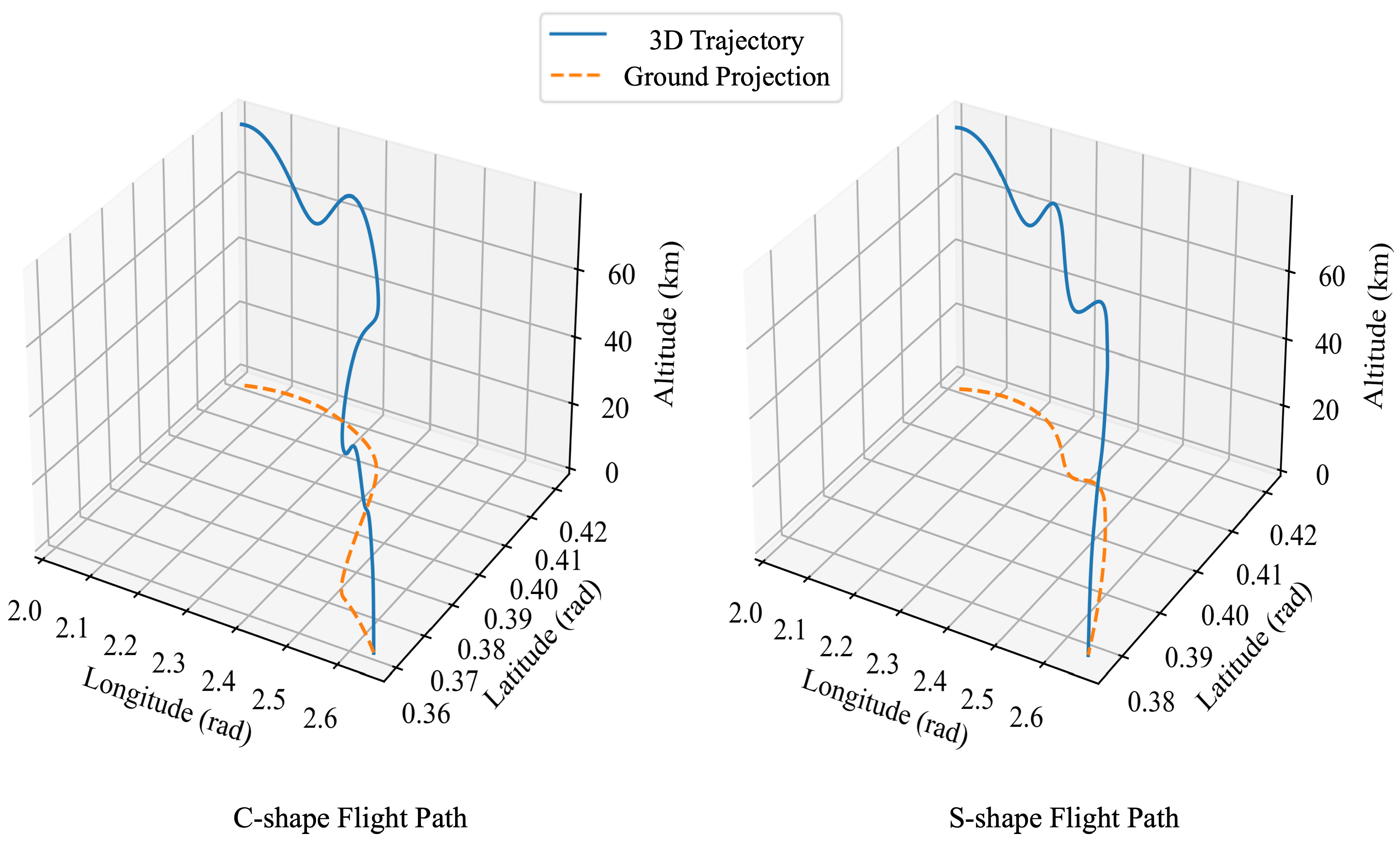
5.1. Dataset Generation

A simulated dataset of HGV trajectories is employed in this study, generated utilizing the Dymos library within the OpenMDAO framework [25]. The dataset comprises 1440 skip-glide trajectories, evenly distributed between lateral C-shaped and S-shaped maneuvers [1]. Each trajectory has an average duration of 891s and encompasses six attributes: altitude, longitude, latitude, velocity, azimuth angle, and flight path angle. The parameters pertaining to the hypersonic vehicle utilized in the simulations are summarized in

Table 1. Hypersonic Glide Vehicle Simulation Parameters.

Parameter	Symbol	Value
Altitude	h	70 $\mathrm{k}$$\mathrm{m}$ to 80 $\mathrm{k}$$\mathrm{m}$
Velocity	v	5000 m s−1 to 6000 m s−1
Flight Path Angle	$\gamma$	0° to 0.2°
Mass	m	$807.2$ kg
Surface Area	S	$0.4839$ m2
Atmospheric Density	$\rho$	The U.S. Standard Atmosphere 1976
Aerodynamic Drag Coef.	$C_D$	$(0.0509-0.0006M_{\alpha })\alpha$
Aerodynamic Lift Coef.	$C_L$	$0.1345-0.012M_{\alpha }+3.7155\times {10}^{-4}{M}_{\alpha }^2+(0.0011-5.6815\times {10}^{-5}{M}_{\alpha }+1.6309\times {10}^{-6}{M}_{\alpha }^2){\alpha }^2$

[26].

5.2. Data Normalization

To mitigate the influence of disparate data dimensions on model training and prediction, and to prevent overfitting, data normalization is performed on each feature independently using the following equation:

$$x^{\prime }={\displaystyle \frac{x-x_{min}}{x_{max}-x_{min}}}$$

(25)

where x is the time series data, $x^{\prime }$ represents the normalized data, $x_{min}$ and $x_{max}$ are the minimum and maximum values of the corresponding feature, respectively. The original data can be restored using the inverse transformation:

$$x=x^{\prime }(x_{max}-x_{min})+x_{min}$$

(26)

5.3. Training and Testing Sets

To assess the model’s performance and generalization ability under varying data scales, the dataset is divided into training and testing sets. We create three different training sets:

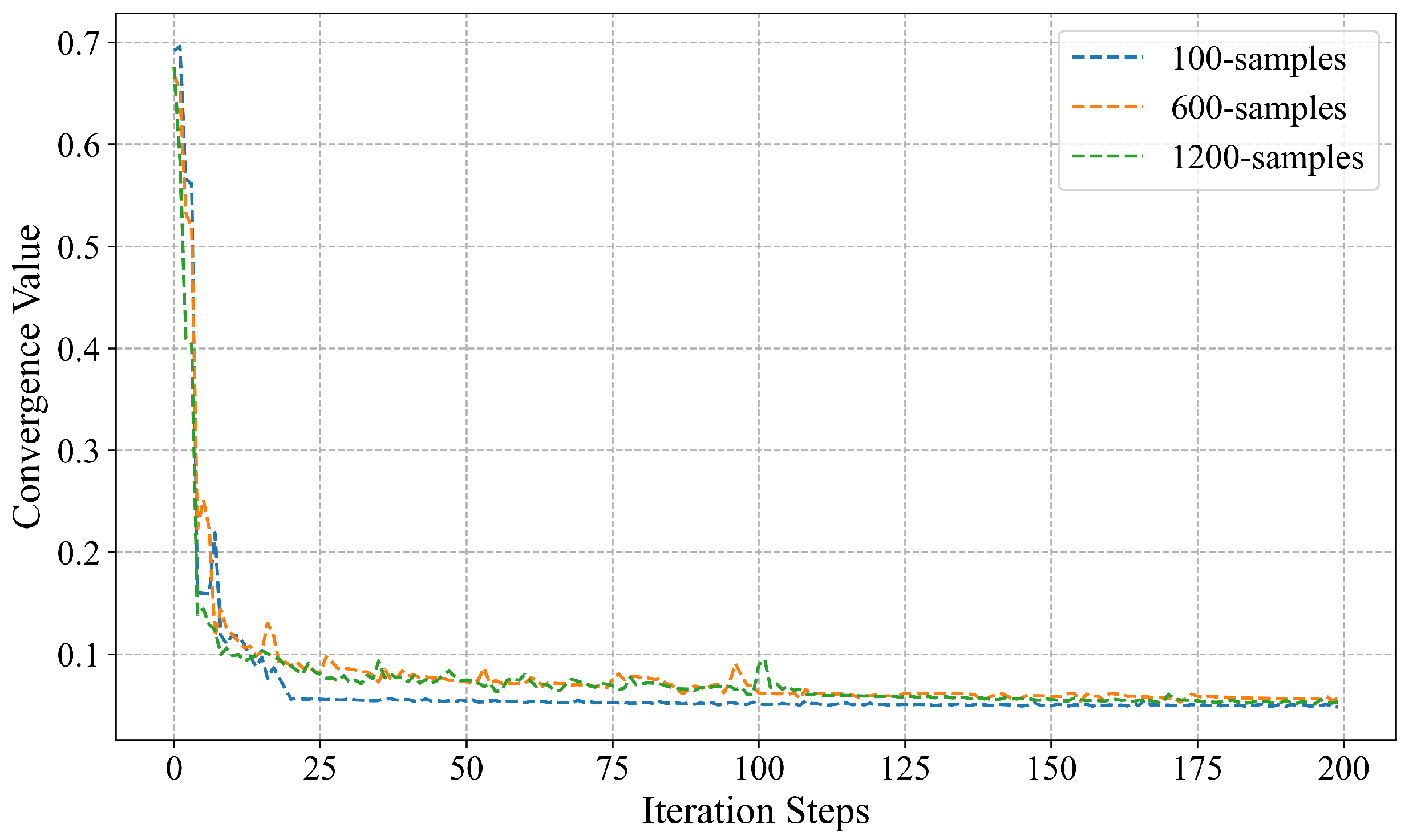
• 100-samples: 100 trajectories randomly selected trajectories for limited data scenarios.
• 600-samples: 600 trajectories randomly selected trajectories for medium data scales.
• 1200-samples: 1200 trajectories randomly selected for sufficient data conditions.

Each training set is further split into 90% for training and 10% for validation. In addition to the validation set, for each training set, a separate testing set consisting of 20% of the respective training set size is generated.

6. Experiments

In this section, we conduct a series of experiments based on the simulated HGV trajectory dataset described in Section 5, focusing on predicting the 100 s trajectory based on 100 s of observed data. We aim to demonstrate the following key advantages of PhysNODE:

• Improved Accuracy: We quantify the prediction accuracy of PhysNODE compared to state-of-the-art trajectory prediction models, especially under limited data scenarios.
• Enhanced Stability: We investigate the generalization ability of PhysNODE trained with different data scales, demonstrating its stability in predicting trajectories.
• Effective Physics Integration: We analyze the impact of incorporating physics knowledge on the prediction performance, particularly in capturing the complex aerodynamic characteristics of HGVs.

6.1. Experimental Setup

6.1.1. Evaluation Metrics

We employ two standard metrics to evaluate the prediction performance of the models:

• Mean Absolute Error (MAE): Measures the average absolute difference between the predicted and ground truth values for longitude, latitude, and altitude.
• Mean Squared Error (MSE): Measures the average squared Euclidean distance between the predicted and ground truth trajectories, reflecting the overall accuracy of trajectory prediction.

6.1.2. Compared Methods

To validate the effectiveness of the proposed PhysNODE model, several representative deep learning models for trajectory prediction are selected as benchmarks for comparison:

• Informer [27]: Informer is a Transformer-based long sequence prediction model. It enhances the efficiency and accuracy of Transformer for long sequence prediction by introducing the probsparse self-attention mechanism and self-distillation technique. Informer can capture long-range dependencies in sequences, making it suitable for predicting hypersonic trajectories with complex aerodynamics.
• LSTM [28]: As a widely adopted and classical deep learning model, LSTM has become a prominent benchmark for evaluating the performance of sequence models, particularly in the realm of trajectory prediction. Its ability to understand long-term patterns from past movements and recognize complex temporal trends makes it effective for this task.
• LSTNet [29]: LSTNet is an integrated time series prediction model that combines 1D CNN, LSTM, and periodic regression components. By utilizing multi-scale convolutions to capture both short-term and long-term features, and leveraging LSTM to memorize long-term dependencies, the model’s performance is further enhanced through skip connections and periodic components. LSTNet is capable of effectively handling complex time series data, making it suitable for predicting glider trajectories.
• Transformer [8]: Transformer, known for its success in language processing, has also proven useful for predicting time series, like trajectories. This is because its special attention mechanism helps it find hidden patterns and connections within data, even across long ranges, enhancing its ability to accurately interpret complex trajectories.
• PhyTransformer [10]: PhyTransformer is a variant of Transformer model that incorporates physics equations as regularization terms in the loss function to penalize prediction results that violate physical laws, thus enhancing the accuracy of the HGV trajectory prediction.
• NODE [15]: NODE is a trajectory prediction model based on Neural ODEs. It utilizes a variational encoder to learn the differential equations of trajectories and generates trajectory predictions through ODE solvers. NODE effectively captures the continuity and smoothness of trajectories but do not directly utilize physics knowledge constraints during the modeling process, relying on a data-driven learning approach.
• PhysNODE-Path: This model extends PhysNODE by incorporating additional path constraints derived from intention inference. Assuming the defender has knowledge of the HGV’s intended target (a realistic assumption in certain scenarios), the following information can be inferred:

  -

  ${\psi }_{target}\left(t\right)$: the azimuth angle of the HGV’s flight direction relative to the target at time t

  -

  $d_{target}\left(t\right)$: the distance between the HGV and the target at time t.

  The two quantities ${\psi }_{target}\left(t\right)$ and $d_{target}\left(t\right)$ are then concatenated with the original observed state vector ${\mathbf{s}}_{obs\left(t\right)}$ (Equation (5)) to form an augmented state vector:

  $${\mathbf{s}}_{obs}^{\prime }\left(t\right)=\mathrm{cat}([{\psi }_{target}\left(t\right),d_{target}\left(t\right)],{\mathbf{s}}_{obs\left(t\right)})$$

  (27)
  This augmented state vector ${\mathbf{s}}_{obs}^{\prime }\left(t\right)$, which includes both the original observed features and the inferred path constraints, is then fed into the Neural Network Prediction module of the PhysNODE (Algorithm 1). By incorporating these additional path constraints, PhysNODE-Path aims to improve the prediction accuracy. This model can be considered a specialized variant of PhysNODE. Therefore, its performance will be analyzed alongside PhysNODE in the subsequent experimental sections. We utilize PhysNODE-Path to showcase the extensibility of the PhysNODE framework, demonstrating its capacity to integrate additional domain-specific information for enhanced prediction.

6.2. Model Convergence Analysis

Model convergence analysis verifies the stability of the PhysNODE training process and its ability to reach a solution. During training, we record and plot the values of the training loss function as a loss curve, as shown as in Figure 4. Within the figure, the distinct lines represent the 100-samples (blue), 600-samples (orange), and 1200-samples (green) training sets.

The results show that the training loss of the PhysNODE model consistently decreases with the increase in the number of training epochs. The loss stabilizes after around 25 epochs and remains steady across all three training sets by epoch 125. This consistent convergence across training sets of varying scales indicates the stability of the model.

6.3. Case Study

A 3D case study is presented to visually demonstrate the predictive capabilities of the PhysNODE model. As depicted in Figure 5, a representative hypersonic trajectory featuring a skip-S-shape maneuver is selected. Using a sequence of observed trajectory data points (red line in the figure), models forecasts the future path of the vehicle. Predictions from different models are distinguished using distinct colors. Meanwhile, The predicted trajectories are compared against the ground truth trajectory.

The experimental results illustrate that the PhysNODE and PhysNODE-Path can accurately predict the 3D trajectory of the hypersonic glider, with the predicted trajectory closely aligning with the ground truth. Notably, our model showed better performance in predicting latitude and longitude but doesn’t do as well in predicting altitude. The reasons for this difference will be explained in Section 6.7.

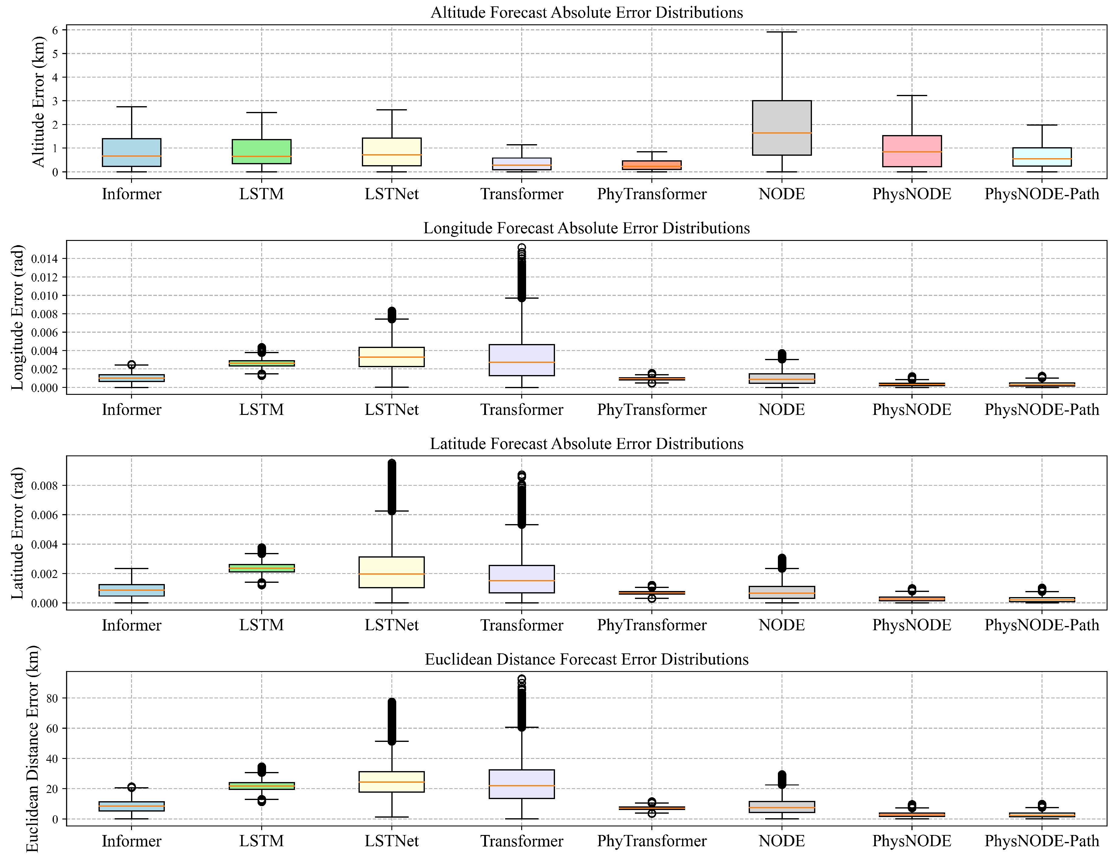
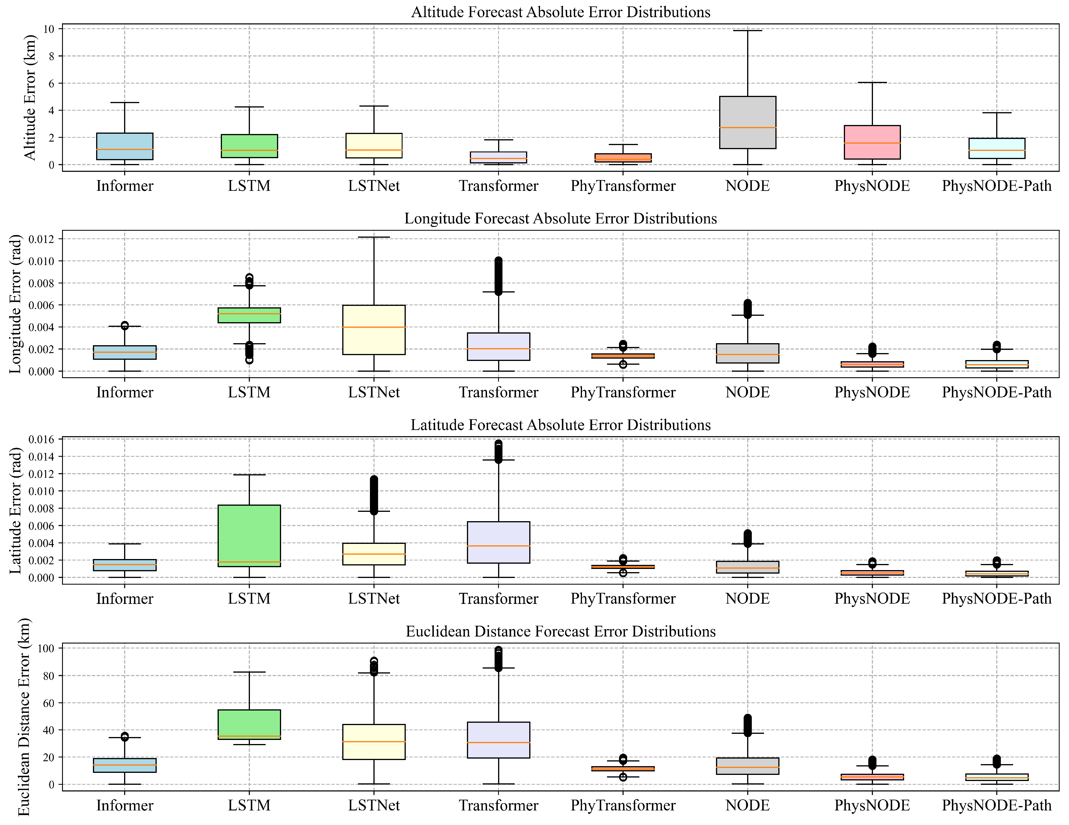
6.4. Model Performance Comparison Analysis

To evaluate the performance of the HGV trajectory prediction models, we train the eight models (Informer, LSTM, LSTNet, Transformer, PhyTransformer, NODE, PhysNODE and PhysNODE-Path) on the three different training sets (100, 600, and 1200 samples). This allows us to assess not only the accuracy of each model but also its ability to generalize from varying amounts of training data. We analyze the prediction errors of four key features: altitude, longitude, latitude, and Euclidean distance (the distance between the true position and the predicted position). Box plots (Figure 6, Figure 7 and Figure 8) are used to visualize and analyze the prediction results on corresponding test sets, which reveal the following performance characteristics for each model.

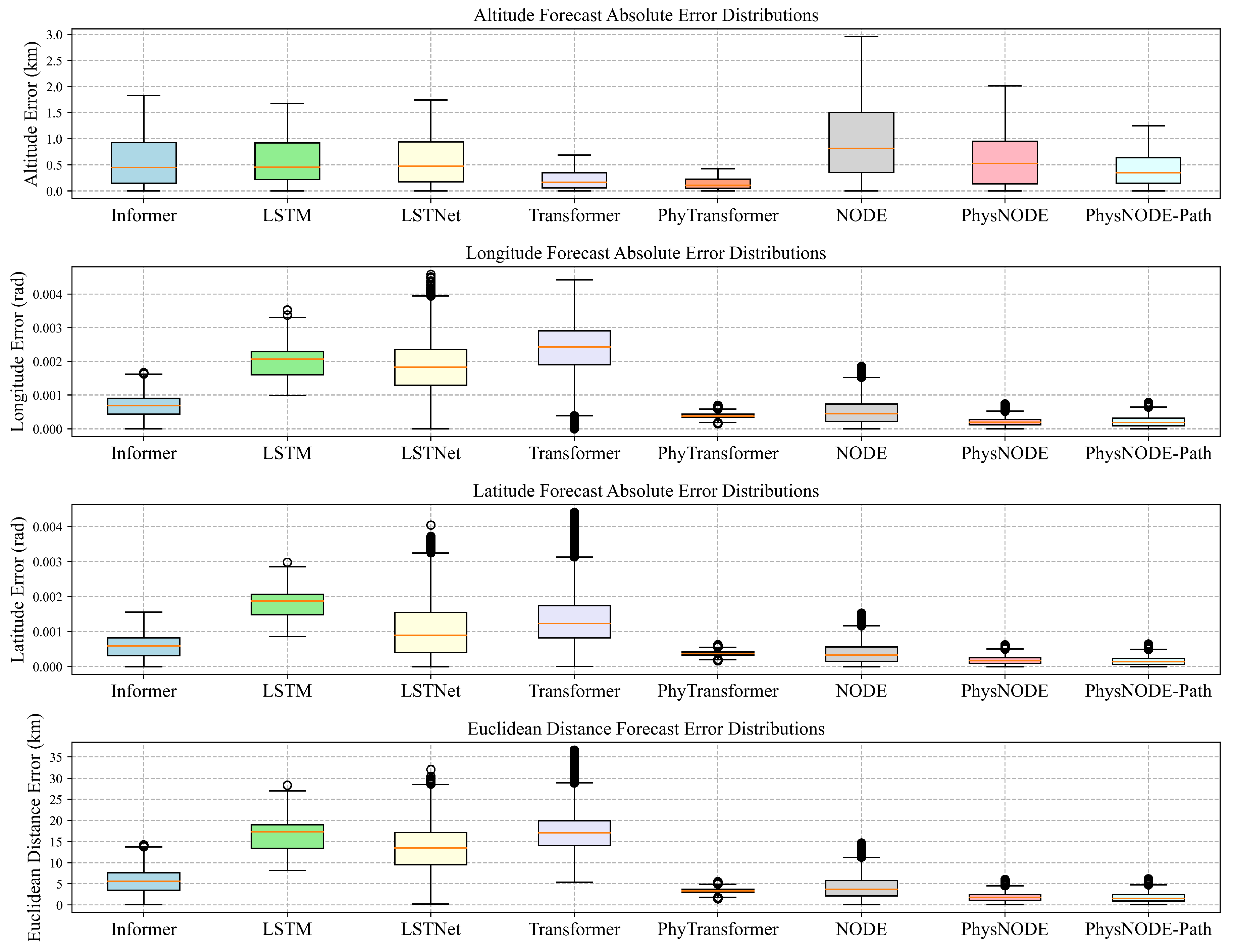
• Informer: The performance of Informer varies noticeably with different data sizes. While it shows relatively accurate altitude predictions, the average altitude error increase from 0.539 km (1200 samples) to 0.809 km (600 samples) and finally to 1.348 km (100 samples). However, Informer encounters troubles in accurate longitude and latitude predictions, particularly with limited training data. With 1200 samples, the average longitude and latitude errors were 0.00067 and 0.00058 radians, respectively. These errors increased to 0.001697 and 0.001465 radians with 100 samples. There is a significant performance gap. The box plots for Informer get wider with less data, meaning its predictions are more uncertain. This suggests that Informer lacks the ability in learning the complex physical dependencies inherent in hypersonic trajectories when trained with limited data.
• LSTM: LSTM consistently underperforms across all evaluation metrics and data scales, indicating a significant sensitivity to limited training data. This suggests a poor ability to generalize and learn the complex dynamics of hypersonic trajectories. Specifically, the average altitude error is already high with 1200 samples at 0.546 km, but it increases to 0.814 km with 600 samples and then to 42.838 km with only 100 samples. Similarly, both longitude and latitude predictions exhibit poor accuracy across all data scales, with average errors remaining above 0.002 radians even when trained on 1200 samples. This poor performance is mirrored in the Euclidean distance errors, which are consistently the highest among all models, reaching 42.84 km with 100 samples. Meanwhile, its box plots are very wide, meaning its predictions are highly dispersed.
• LSTNet: LSTNet demonstrates some improvement over LSTM, particularly in longitude and latitude predictions when trained on larger datasets. However, its overall performance remains inadequate, especially with limited training data. With 1200 samples, LSTNet achieves average errors of 0.001814 radians for longitude and 0.001064 radians for latitude, outperforming LSTM in these aspects. However, it faces difficult in altitude prediction, yielding an average error of 0.548 km. This inconsistency across different prediction targets is further amplified with smaller datasets. In 600 samples dataset, LSTNet’s performance advantage over LSTM diminished, with average errors increasing to 0.003365 radians (longitude), 0.002187 radians (latitude), and 0.830 km (altitude). This trend continued with 100 samples, where LSTNet’s errors are 0.003981 radians (longitude), 0.002846 radians (latitude), and 1.353 km (altitude). The Euclidean distance errors for LSTNet are consistently high across all data scales, indicating poor overall prediction accuracy. Additionally, its wider error distributions in the box plots suggest a lack of stability in its predictions. Overall, while LSTNet shows some potential with larger datasets, its performance degrads significantly with limited data.
• Transformer: While Transformer achieves a higher accuracy in altitude prediction, especially with larger datasets (0.202 km average error for 1200 samples), its performance in predicting longitude and latitude remains moderate, the box plots is wider and exhibited instability with smaller datasets. For example, with 1200 samples, the average longitude and latitude errors are 0.002384 and 0.001394 radians, respectively. These errors grow to 0.003216 and 0.001761 radians with 600 samples and further increase to 0.002426 and 0.004292 radians with 100 samples. This pattern is also reflected in the Euclidean distance error, which rises from 17.52 km (1200 samples) to 24.25 km (600 samples) and 33.50 km (100 samples). This indicates that while Transformer shows initial success for altitude prediction, its ability to model the full features of hypersonic trajectories is restricted.
• PhyTransformer: The physics-informed PhyTransformer consistently outperformed the standard Transformer model in all metrics and across all data scales. This highlights the benefits of incorporating physics-based constraints to guide the learning process, especially when data is limited. For instance, with only 100 samples, PhyTransformer achieves remarkably low average errors of 0.001391 radians (longitude), 0.001235 radians (latitude), and 0.475 km (altitude) compared to the standard Transformer’s errors of 0.002426 radians, 0.004292 radians, and 0.539 km, respectively. Similarly, the Euclidean distance errors are significantly lower for PhyTransformer across all data scales and the box plot is very narrow, demonstrating its superior ability to accurately capture the dynamics of hypersonic trajectories.
• NODE: Benefiting from its neural ODE framework, NODE outperforms the data-driven models (Informer, LSTM, LSTNet) in most cases. However, its overall performance falls short of the physics-informed PhyTransformer and PhysNODE, especially with small dataset. For instance, while it achieves relatively low average errors in longitude (0.000511 radians), latitude (0.000385 radians), and altitude (0.927 km) with 1200 samples, these errors increase considerably when trained on 600 samples and even more so with 100 samples. This trend is also apparent in the Euclidean distance errors. Meanwhile, its box plot is very wide in altitude attribute. These results highlight the potential of neural ODEs for trajectory prediction, while also emphasizing the importance of exploring further integration of physics-based constraints within this framework to enhance accuracy and stability.
• PhysNODE: PhysNODE consistently displays remarkable performance in predicting hypersonic trajectories across various training data scales, demonstrating its ability to maintain accuracy even with limited data. With 1200 training samples, PhysNODE achieves impressive results, including average errors of 0.000207 radians for longitude, 0.000180 radians for latitude, and 0.574 km for altitude, resulting in the lowest average Euclidean distance error of 1.850 km among all models. Decreasing the training data to 600 samples still yields strong performance, with average errors of 0.000332 radians (longitude), 0.000289 radians (latitude), and 0.919 km (altitude), resulting in an average Euclidean distance error of 2.961 km. Even with further reduction to 100 training samples, PhysNODE continues to excel, achieving average errors of 0.000452 radians (longitude), 0.000396 radians (latitude), and 1.163 km (altitude), with an average Euclidean distance error of 5.553 km. Although it does not achieve optimal results in altitude prediction, and the box plot is wider, the results across various data scales still highlight the robustness of PhysNODE in leveraging data-driven learning with physical knowledge, enabling accurate predictions of hypersonic trajectory dynamics and effective generalization with limited training data.
  In addition, PhysNODE-Path consistently outperforms the standard PhysNODE. With 100 training samples, PhysNODE-Path achieves an average Euclidean distance error of 5.442 km. This trend of slight improvement with PhysNODE-Path continues with 600 training samples (2.827 km) and 1200 training samples (1.784 km). This small but consistent improvement highlights the flexibility of the PhysNODE framework, which allows for the integration of additional domain-specific information, such as knowledge about the target, to enhance predictive accuracy.

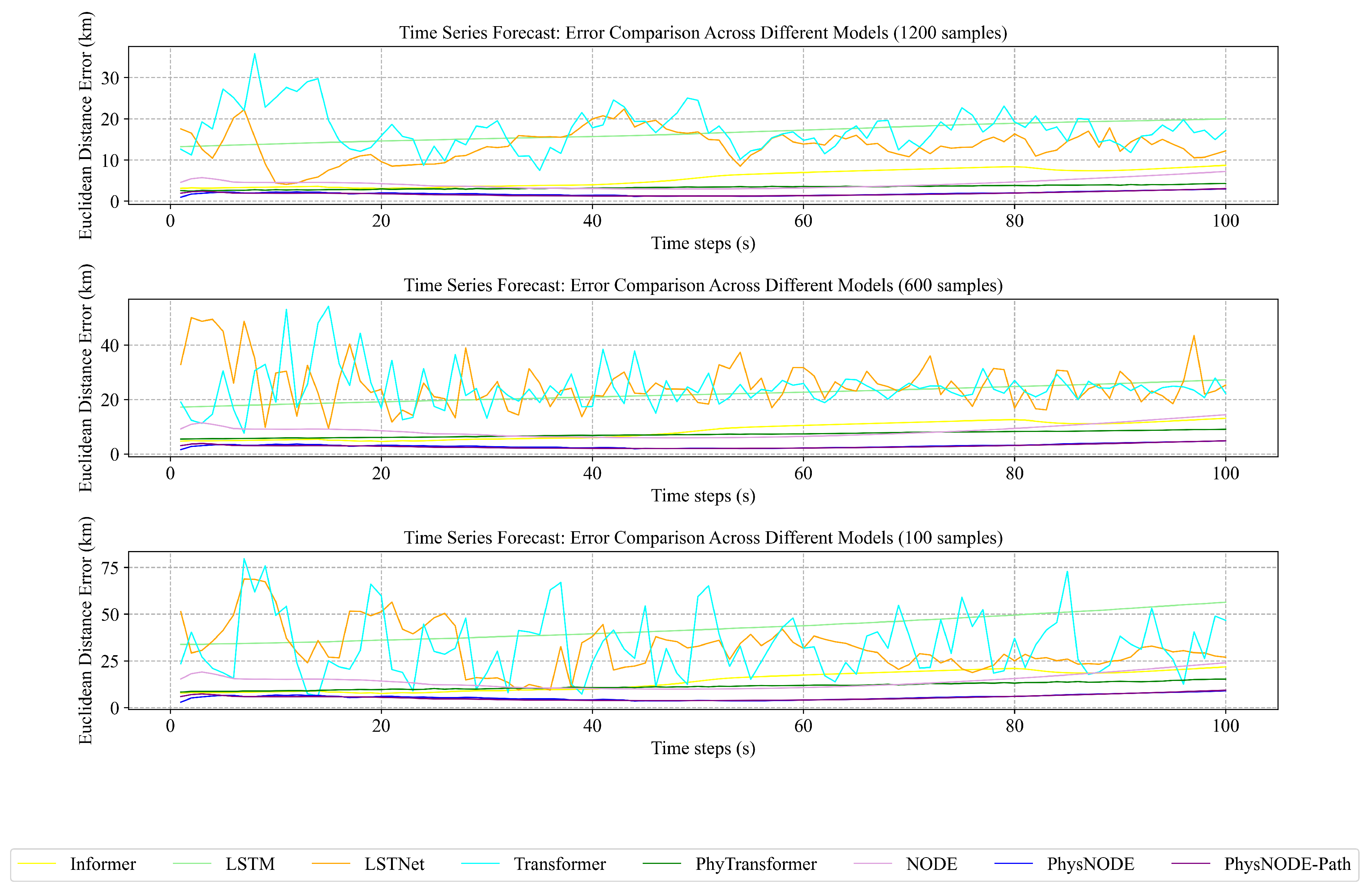
6.5. Forecast Accuracy over Time

Based on the Euclidean distance error plots in Figure 9, which shows the average distance errors calculated over the test sets, we can evaluate the predictive capabilities of each model across various prediction horizons.

• Informer: Informer demonstrates inconsistent performance in predicting hypersonic trajectories over time. With 1200 training samples, the Euclidean distance error initially remains relatively low but exhibits noticeable fluctuations and a gradual upward trend as the prediction horizon extended. Reducing the training data to 600 samples let to a higher initial error and greater instability, with more pronounced fluctuations throughout the prediction horizon. This instability is further exacerbated with only 100 training samples, where the error increases rapidly and fluctuated significantly over time.
• LSTM: LSTM consistently exhibited poor performance across all data scales. With 1200 training samples, the error is already high at the start and rapidly increased with increasing prediction time. This trend is even more pronounced with 600 and 100 training samples, indicating a severe lack of generalization ability, regardless of data availability.
• LSTNet: LSTNet also displays high errors and large fluctuations across all data scales. While increasing the training data from 100 to 1200 samples let to a slight reduction in the overall error, the model still difficult to maintain accuracy over longer prediction horizons.
• Transformer: Transformer shows a very unstable error pattern across all training sets and throughout the entire prediction horizon. This volatility, resembling that observed with LSTM, suggests that neither model possesses the capability for stable and consistent prediction.
• PhyTransformer: PhyTransformer consistently exhibits more stable performance than the standard Transformer across all data scales. With 1200 samples, it maintained a relatively low and stable error throughout the prediction horizon. While a slight increase in error is observed with 600 and 100 samples, the overall error remained significantly lower and more stable than the standard Transformer, indicating the benefit of incorporating physics constraints.
• NODE: With 1200 training samples, NODE exhibited a relatively low initial error and a relatively smooth error trajectory over the prediction horizon. However, as the training data decreased to 600 and 100 samples, both the initial error and the rate of error increase over time became more pronounced. This suggests that while the neural ODE framework can capture some temporal dependencies, its performance is still sensitive to data availability.
• PhysNODE: Both PhysNODE and PhysNODE-Path consistently show the smallest errors and the most reliable predictions across all dataset sizes. Even with limited training data (only 100 samples), both models maintain accurate and consistent predictions throughout the entire forecasting period. This robust stability, along with their high accuracy, demonstrates the advantage of combining physics-based knowledge with deep learning for dependable and accurate hypersonic trajectory prediction. Additionally, PhysNODE-Path, which incorporates additional path constraints, shows slightly better accuracy than standard PhysNODE, especially in the first half of the flight. This result reveals the benefit of including path information for improving the reliability of predictions.

6.6. Benefits of Physics-Informed Modeling

PhysNODE outperforms other models in predicting HGV trajectories, primarily because it integrates physics-based knowledge. By using neural networks to learn the aerodynamic parameters, PhysNODE ensures its predictions are physically realistic. Compared to models that don’t incorporate physics (like Informer, LSTM, LSTNet, and Transformer), PhysNODE consistently achieves better accuracy across different datasets and prediction metrics. Furthermore, this study also highlights the strength of using neural ODEs for trajectory prediction. Even without explicit physics knowledge, a simple neural ODE model performs better than most other models.

It is noteworthy that, PhyTransformer, which incorporates physics only in its loss function, shows improved accuracy compared to Transformer. This highlights the benefit of integrating physics. Both PhyTransformer and PhysNODE demonstrate more stable predictions, especially when data is limited. This improved stability is crucial for real-world applications where data might be scarce. However, PhysNODE consistently shows more accuracy than PhyTransformer in predicting trajectories. This demonstrates the effectiveness of our approach in integrating physical knowledge into the model.

6.7. Relationship between Prediction Accuracy and Variable Complexity

The initial design of PhysNODE is intended to enhance the prediction capability for complex variables by embedding physical laws. Our study demonstrates that PhysNODE excels in predicting longitude and latitude. The prediction of these variables involves multiple nonlinear factors and complex dynamic processes. PhysNODE effectively leverages its physics-embedded structure and the robust learning capabilities of neural networks to capture these intricate relationships.

Based on Equation (1), the prediction of longitude ($\lambda$) and latitude ($\varphi$) is governed by the following equations:

$${\displaystyle \frac{d\lambda }{dt}}={\displaystyle \frac{vcos\gamma sin\psi }{rcos\varphi }}$$

(28)

$${\displaystyle \frac{d\varphi }{dt}}={\displaystyle \frac{vcos\gamma cos\psi }{r}}$$

(29)

These equations include trigonometric functions and the Earth’s radius, reflecting the intricate dependencies on multiple flight parameters such as velocity (v), flight path angle ($\gamma$), and heading angle ($\psi$).

However, for simpler variables like altitude (h), the prediction is governed by a more straightforward equation:

$${\displaystyle \frac{dh}{dt}}=vsin\gamma$$

(30)

The change in altitude primarily depends on velocity and flight path angle, involving fewer complex interactions. This difference in variable complexity explains why the relative advantages of PhysNODE are less apparent in predicting altitude. This phenomenon suggests that the PhysNODE architecture is more suited to tasks requiring multi-angle information integration for complex predictions, whereas its potential advantages are not fully realized in simpler tasks.

7. Conclusions

This paper introduces PhysNODE, a novel physics-embedded neural ODE framework designed to enhance HGV trajectory prediction. PhysNODE actively leverages physical knowledge to guide the learning process, resulting in improved accuracy, stability, and generalization, especially in scenarios with limited data. Furthermore, as demonstrated by the PhysNODE-Path variant, the framework exhibits promising extensibility, allowing for the integration of additional domain-specific information to further enhance predictive accuracy.

Key innovations of PhysNODE include:

• Decomposing the HGV motion equations into observable and predictable components, allowing for targeted prediction of unobservable aerodynamic parameters.
• Utilizing a hybrid neural network architecture (CNN + MLP) to effectively learn and predict these aerodynamic parameters.
• Encapsulating the learned physical knowledge within an ODE block, integrated with an ODE solver for continuous-time trajectory prediction.

Our experimental evaluation on simulated HGV trajectory datasets demonstrates the superior performance of PhysNODE compared to state-of-the-art data-driven and physics-informed methods. PhysNODE consistently achieves the highest comprehensive prediction accuracy and stability across different data scales, particularly excelling under limited data conditions. This robust performance highlights the effectiveness of our physics-embedded approach in handling the complex dynamics of HGV trajectories.

Despite its promising results, PhysNODE relies on accurate knowledge of the underlying HGV dynamics equations, which can be complex and include various constraints, potentially impacting the model’s performance in real-world scenarios. Additionally, the current implementation of PhysNODE focuses on the HGV trajectory state without considering control inputs in vehicles. Incorporating this factor could further enhance the model’s predictive capabilities.

Several avenues for future research exist:

• Investigating the incorporation of additional physical constraints, such as thermodynamics, to enhance the model’s accuracy and physical consistency. Exploring alternative methods for embedding physics knowledge within the Neural ODE framework, such as Hamiltonian or Lagrangian mechanics, could also be beneficial.
• Evaluating PhysNODE’s robustness to noise, uncertainties, and incomplete data is crucial for its practical applicability.
• Extending the principles of PhysNODE to predict trajectories for other vehicles, such as the subsonic unpowered gliding vehicle (SUGV) [30]. Adapting the model to handle various flight dynamics and incorporating relevant physical constraints would be key challenges in this extension.

References

1. Li, G.; Zhang, H.; Tang, G. Maneuver characteristics analysis for hypersonic glide vehicles. Aerosp. Sci. Technol. 2015, 43, 321–328. [Google Scholar]
2. Law, Y.W.; Gliponeo, J.J.; Singh, D.; McGuire, J.; Liang, J.; Ho, S.Y.; Slay, J. Detecting and tracking hypersonic glide vehicles: A cybersecurity-engineering analysis of academic literature. In Proceedings of the 18th International Conference on Cyber Warfare and Security, Baltimore County, MD, USA, 9–10 March 2023; pp. 189–198. [Google Scholar]
3. Le, W.; Liu, H.; Zhao, R.; Chen, J. Attitude control of a hypersonic glide vehicle based on reduced-order modeling and NESO-assisted backstepping variable structure control. Drones 2023, 7, 119. [Google Scholar] [CrossRef]
4. Zhang, H.B.; Xie, Y.; Chan, K.J. Investigation on trajectory prediction of maneuverable target. Mod. Def. Technol. 2011, 39, 26–31. [Google Scholar]
5. Sun, L.; Yang, B.; Ma, J. Trajectory prediction in pipeline form for intercepting hypersonic gliding vehicles based on LSTM. Chin. J. Aeronaut. 2023, 36, 421–433. [Google Scholar] [CrossRef]
6. Halim, C.J.; Kawamoto, K. 2D convolutional neural markov models for spatiotemporal sequence forecasting. Sensors 2020, 20, 4195. [Google Scholar] [CrossRef] [PubMed]
7. Kiranyaz, S.; Avci, O.; Abdeljaber, O.; Ince, T.; Gabbouj, M.; Inman, D.J. 1D convolutional neural networks and applications: A survey. Mech. Syst. Signal Process. 2021, 151, 107398. [Google Scholar] [CrossRef]
8. Han, K.; Xiao, A.; Wu, E.; Gou, J.; Xu, C.; Wang, Y. Transformer in Transformer. In Proceedings of the 35th Advances in Neural Information Processing Systems, Online, 6–14 December 2021; pp. 15908–15919. [Google Scholar]
9. Lim, B.; Zohren, S. Time-series forecasting with deep learning: A survey. Phys. Eng. Sci. 2021, 379, 20200209. [Google Scholar] [CrossRef] [PubMed]
10. Ren, J.; Wu, X.; Liu, Y.; Ni, F.; Bo, Y.; Jiang, C. Long-term trajectory prediction of hypersonic glide vehicle based on physics-informed transformer. IEEE Trans. Aerosp. Electron. Syst. 2023, 59, 9551–9561. [Google Scholar] [CrossRef]
11. Djeumou, F.; Neary, C.; Goubault, E.; Putot, S.; Topcu, U. Neural networks with physics-informed architectures and constraints for dynamical systems modeling. In Proceedings of the 4th Learning for Dynamics and Control Conference, Palo Alto, CA, USA, 23–24 June 2022; pp. 263–277. [Google Scholar]
12. Hao, Z.K.; Liu, S.M.; Zhang, Y.; Ying, C.Y.; Feng, Y.; Su, H.; Zhu, J. Physics-informed machine learning: A survey on problems, methods and applications. arXiv 2022, arXiv:2211.08064. [Google Scholar]
13. Meng, C.; Niu, H.; Habault, G.; Legaspi, R.; Wada, S.; Ono, C.; Liu, Y. Physics-informed long-sequence forecasting from multi-resolution spatiotemporal data. In Proceedings of the 31th International Joint Conference on Artificial Intelligence, Vienna, Austria, 23–29 July 2022; pp. 2189–2195. [Google Scholar]
14. Chen, Y.; Huang, D.; Zhang, D.; Zeng, J.; Wang, N.; Zhang, H.; Yang, J. Theory-guided hard constraint projection (HCP): A knowledge-based data-driven scientific machine learning method. J. Comput. Phys. 2021, 445, 110624. [Google Scholar] [CrossRef]
15. Chen, R.T.Q.; Rubanova, Y.; Bettencourt, J.; Duvenaud, D.K. Neural ordinary differential equations. In Proceedings of the 32th Advances in Neural Information Processing Systems, Montreal, QC, Canada, 2–12 December 2018; p. 31. [Google Scholar]
16. Berkani, S.; Guermah, B.; Zakroum, M.; Ghogho, M. Spatio-temporal forecasting: A survey of data-driven models using exogenous data. IEEE Access 2023, 11, 75191–75214. [Google Scholar] [CrossRef]
17. Zhang, J.; Xiong, J.; Li, L.; Xi, Q.; Chen, X.; Li, F. Motion state recognition and trajectory prediction of hypersonic glide vehicle based on deep learning. IEEE Access 2022, 10, 21095–21108. [Google Scholar] [CrossRef]
18. Xie, Y.; Zhuang, X.; Xi, Z.; Chen, H. Dual-channel and bidirectional neural network for hypersonic glide vehicle trajectory prediction. IEEE Access 2021, 9, 92913–92924. [Google Scholar] [CrossRef]
19. Liu, Y.; Xie, Y.; Li, W.; Zhang, Y. Real-time trajectory prediction for hypersonic glide vehicle based on 3-D flight corridor. In Proceedings of the 6th International Conference on Automation, Control and Robotics Engineering, Dalian, China, 15–17 July 2021; pp. 598–603. [Google Scholar]
20. Li, M.; Zhou, C.; Shao, L.; Lei, H.; Luo, C. Intelligent trajectory prediction algorithm for reentry glide target based on intention inference. Appl. Sci. 2022, 12, 10796. [Google Scholar] [CrossRef]
21. Azencot, O.; Erichson, N.B.; Lin, V.; Mahoney, M.W. Forecasting sequential data using consistent koopman autoencoders. In Proceedings of the 37th International Conference on Machine Learning, Online, 12–18 July 2020; pp. 475–485. [Google Scholar]
22. Jin, M.; Zheng, Y.; Li, Y.F.; Chen, S.H.; Yang, B.; Pan, S.R. Multivariate time series forecasting with dynamic graph neural odes. IEEE Trans. Knowl. Data Eng. 2022, 35, 9168–9180. [Google Scholar] [CrossRef]
23. Asikis, T.; Böttcher, L.; Antulov-Fantulin, N. Neural ordinary differential equation control of dynamics on graphs. Phys. Rev. Res. 2022, 4, 013221. [Google Scholar] [CrossRef]
24. Lu, P.; Forbes, S.; Baldwin, M. Gliding guidance of high L/D hypersonic vehicles. In Proceedings of the AIAA Guidance, Navigation, and Control (GNC) Conference, Boston, MA, USA, 19–22 August 2013; p. 4648. [Google Scholar]
25. Falck, R.; Gray, J.S.; Ponnapalli, K.; Wright, T. A Python package for optimal control of multidisciplinary systems. J. Open Source Softw. 2021, 6, 2809. [Google Scholar] [CrossRef]
26. Zhang, K.; Xiong, J.; Fu, T. Multi-model estimation of HGV based on coupled aerodynamic parameters. J. Beijing Univ. Aeronaut. Astronaut. 2018, 44, 2156–2164. [Google Scholar]
27. Zhou, H.; Zhang, S.; Peng, J.; Zhang, S.; Li, J.X.; Xiong, H.; Zhang, W.C. Informer: Beyond efficient transformer for long sequence time-series forecasting. In Proceedings of the 35th AAAI conference on artificial intelligence, Online, 2–9 February 2021; p. 1110. [Google Scholar]
28. Yu, Y.; Si, X.; Hu, C.; Zhang, J.X. A Review of recurrent neural networks: LSTM cells and network architectures. Neural Comput. 2019, 31, 1235–1270. [Google Scholar] [CrossRef]
29. Lai, G.; Chang, W.C.; Yang, Y. Modeling long-and short-term temporal patterns with deep neural networks. In Proceedings of the 41th international ACM SIGIR conference on research & development in information retrieval, New York, NY, USA, 8–12 July 2018; pp. 95–104. [Google Scholar]
30. Mahmood, A.; Rehman, F.; Bhatti, A.I. Trajectory optimization of a subsonic unpowered gliding vehicle using control vector parameterization. Drones 2022, 6, 360. [Google Scholar] [CrossRef]
Figure 1. Typical Maneuvering Trajectories of HGV.
Drones 08 00377 g001
Figure 2. Schematic Overview of PhysNODE.
Drones 08 00377 g002
Figure 3. PhysNODE Framework.
Drones 08 00377 g003
Figure 4. Convergence analysis of PhysODE.
Drones 08 00377 g004
Figure 5. A 3D Trajectory Prediction Case.
Drones 08 00377 g005
Figure 6. Prediction Errors of Models with 1200 Training Samples.
Drones 08 00377 g006
Figure 7. Prediction Errors of Models with 600 Training Samples.
Drones 08 00377 g007
Figure 8. Prediction Errors of Models with 100 Training Samples.
Drones 08 00377 g008
Figure 9. Error Comparison across Different Models over Time.
Drones 08 00377 g009