Finite Time-Adaptive Full-State Quantitative Control of Quadrotor Aircraft and QDrone Experimental Platform Verification

Abstract

This paper proposes a novel adaptive finite-time controller for a quadrotor unmanned aerial vehicle (UAV) model with stochastic perturbations and parameter-unknown terms, under the constraints of a state-constrained system. The controller is designed based on full-state quantization, where the error system is defined to be a function of the quantized error signal. An adaptive method is employed to address the quadrotor UAV system model with nonlinear terms and unknown perturbations. The controller utilizes Barrier Lyapunov function (BLF) bounds with adaptive effective time performance to ensure full-state constraint of the system. The stability of the system is proven using Lyapunov’s stability theorem. The effectiveness of the designed full-state constrained controller for quadrotor UAV based on full-state quantization is verified through a physical experimental simulation platform.

1. Introduction

As one of the classic representatives of UAVs, quadrotor UAVs have many excellent features such as simple structure, various sizes, low cost, easy operation, and strong vertical takeoff and landing capability. It has already possessed an increasingly wide range of applications in different fields such as military, agriculture, and civil [1,2]. In the formation control of quadrotor UAVs, the acquisition of state information needs to rely on the feedback information obtained after communicating with other UAVs for computation, and the states in the controller at this time are quantized information. Therefore, the research on quadrotor UAVs considering full state quantization is also more necessary [3].

In recent years, with advancements in communication technology, the analysis and design of systems with quantized signals have gained significant attention. For quadrotor control, position and attitude control signals are generated by onboard processors and transmitted through communication channels with limited bandwidth [4,5]. Therefore, these signals need to be quantized before transmission. However, the quantization process introduces errors that can exacerbate the inherent nonlinearities of quadrotors, potentially rendering conventional controller designs invalid and leading to issues such as tracking errors and poor transient responses [6,7]. Consequently, considering quantization in the controller design is essential to ensure precise control and system stability, making quantized control indispensable in the control design of quadrotors.

The work in [8] addresses the problem of stabilizing control of discrete time-invariant systems, and for the first time proposes the concept of state quantization, and gives a binding method for sampled-data systems based on the sector-bounded nature of the pair quantizer. In [9], the authors address the problem of adaptive control for multi-channel systems with quantized inputs. They establish a Lipschitz logarithmic quantizer considering packet loss in data transmission, implementing the elimination of quantized errors on a quadrotor UAV and proving its superiority. In [10], the authors address the problem of quadrotor attitude tracking using a quantized control. They employ a hysteretic quantizer to reduce transmission burden and demonstrate the strategy’s effectiveness through experimental results. In [11], the authors propose a finite-time command filtered backstepping adaptive control strategy for quadrotor UAVs with quantized inputs and external disturbances, demonstrating its effectiveness through a numerical example.

Although the above references designed control schemes for state quantized systems, they did not consider the case of state constraints in the system. As a result, the system cannot meet the performance of state constraints under state quantization. Therefore, this article proposes an adaptive full-state quantized control for a quadrotor unmanned aerial vehicle (UAV) with full-state constraint characteristics, which can satisfy the system’s state constraint performance while state quantization is applied. In practical scenarios, systems sometimes have state constraints [12,13]. This is also the case for quadrotor UAV systems, such as the flight trajectory, velocity, acceleration, pitch or yaw angles, which need to be constrained. Barrier Lyapunov functions are an effective method [14] for addressing this. Therefore, for quadrotor UAV systems with state constraints, adaptive control can be combined with barrier Lyapunov functions [15] to build control schemes that satisfy the system’s state constraint conditions. In addition, preset performance functions are also a popular control technique, which converts the system’s tracking error into a specific form to limit the tracking error within a predetermined range. The development and evolution of preset performance functions have gone through three stages. The initial form of the function can be found in the literature [16], which adds the exponential function to the preset performance function to enable the entire function to converge quickly to the preset target value. In [17], this preset performance function was applied to multi-agent systems to maintain the instantaneous performance and stability of the system’s synchronization error.

Over time, the finite-time preset performance function [18] emerged as the second stage of the performance function’s development by changing the exponential part of the initial performance function. In [19], this function was used to solve the quantized tracking control problem of time-delay nonlinear systems and to propose a new barrier function that combines the preset performance function and barrier Lyapunov function to improve the tracking performance of the entire system. Recently, a new finite-time performance function has been proposed, which can dynamically adjust its parameters according to the current tracking error of the system. It is called the self-adjusting finite-time preset performance function [20], representing the third stage of the performance function. In [21], this function was integrated into the barrier Lyapunov function to restrict the system’s state constraints, as it can adapt its parameters to handle different situations and make the designed control method more suitable for practical situations.

Driven by above studies, the novelties of this paper are summarized as follows:

• Based on an adaptive time-varying BLF, we propose a novel adaptive full-state quantization control strategy for a class of quadrotor UAV systems with unknown model parameters and random external disturbances to constrain the states within predefined time-varying boundaries. The proposed control algorithm not only compensates for the quantization effects, but also guarantees sufficient precision.
• To cope with the problem of signal discontinuity that may occur during state quantization, this study proposes an error system based on the definition of the quantization error signal. With this method, the effect of state quantization can be mitigated and the overall performance of the control system can be improved. At the same time, an adaptive control method is used to cope with the nonlinear characteristics and unknown disturbances existing in the system, which is able to adjust the control parameters based on real-time system feedback and enhance the robustness of the system.
• By combining the definition of the filtered tracking error with an adaptive time-varying BLF, the controller design process is simplified. This approach reduces the number of design parameters while achieving full-state constraint performance of the control system, enhancing both tracking accuracy and anti-interference capability. The stability of the proposed scheme is rigorously demonstrated using Lyapunov stability theory, and its effectiveness is validated through physical experimental simulations.

The chapter is organized as follows: Section 2 presents the preparatory knowledge required during the controller design process as well as the relevant lemmas. Section 3 carries out the controller design as well as proving the stability of the system through Lyapunov’s theorem. Section 4 demonstrates the effectiveness of the scheme illustrated in this chapter through physical experimental simulations. Section 5 states the conclusions and summarizes.

2. Problem Formulation and Preliminaries

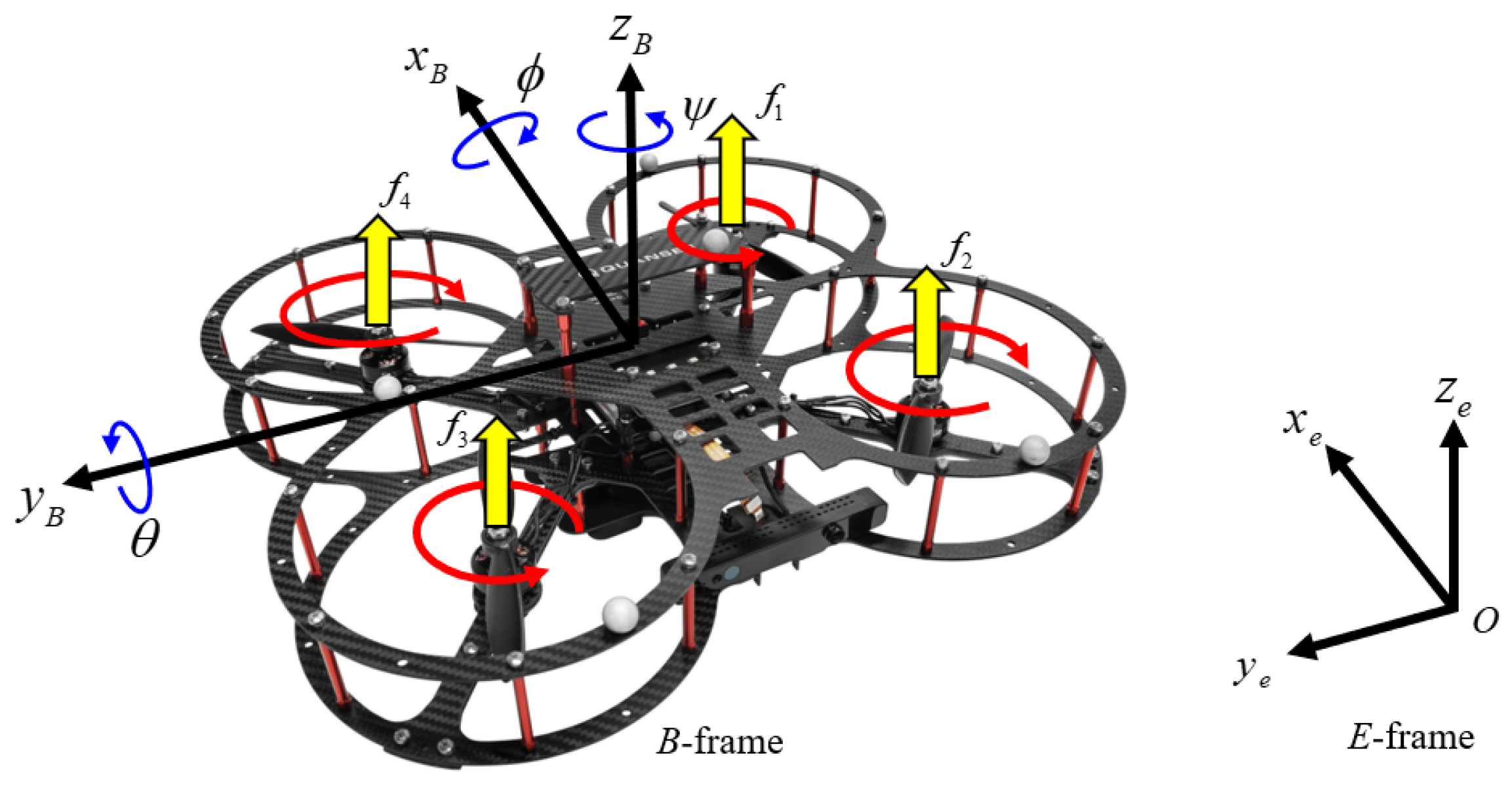
2.1. System Model of Quadrotor

The structure of the quadrotor UAV is shown in Figure 1, where $O{x}_B{y}_B{z}_B$ refers to the Body Frame, $O{x}_e{y}_e{z}_e$ refers to the Earth-fixed Frame, and its general dynamic model is shown in Formula (1), the derivation of which is described in reference [22].

$$\left\{\begin{array}{c}\ddot{x}=(C_{\varphi }{S}_{\theta }{C}_{\psi }+S_{\varphi }{S}_{\psi })U_1-a_1\dot{x}+d_1\hfill \\ \ddot{y}=(C_{\varphi }{S}_{\theta }{S}_{\psi }-S_{\varphi }{C}_{\psi })U_1-a_2\dot{y}+d_2\hfill \\ \ddot{z}=\left(C_{\varphi }{C}_{\theta }\right)U_1-g-a_3\dot{z}+d_3\hfill \\ \ddot{\varphi }=a_4\dot{\theta }\dot{\psi }+a_5\dot{\theta }\Omega -a_6\dot{\varphi }+d_4+U_2\hfill \\ \ddot{\theta }=a_7\dot{\varphi }\dot{\psi }+a_8\dot{\varphi }\Omega -a_9\dot{\theta }+d_5+U_3\hfill \\ \ddot{\psi }=a_{10}\dot{\varphi }\dot{\theta }-a_{11}\dot{\psi }+d_6+U_4\hfill \end{array}\right.,$$

(1)

where $x,y,z$ represent the displacement of quadrotor UAV in the $x_e,y_e,z_e$ directions, respectively, and $\varphi ,\theta ,\psi$ represent the roll angle, pitch angle, and yaw angle, respectively, $S_{•}$ on behalf of $sin(•)$, $C_{•}$ on behalf of $cos(•)$, g is the gravity acceleration, $a_j,j=1,\dots ,11$ are unknown, $\Omega$ denotes the relative speed of the cross-coupled rotor and satisfies $\Omega ={\Omega }_1-{\Omega }_2+{\Omega }_3-{\Omega }_4$ with ${\Omega }_k,k=1,\dots ,4$ being the rotating speed of the propeller, $d_i,i=1,\dots ,6$ denote the bounded external disturbances, and $U_k,k=1,\cdots ,4$ represent the aforementioned control inputs and are defined as follows:

$$\left\{\begin{array}{c}{U}_1=k\left({\Omega }_1^2+{\Omega }_2^2+{\Omega }_3^2+{\Omega }_4^2\right)/m\hfill \\ U_2=lk\left(-{\Omega }_1^2-{\Omega }_2^2+{\Omega }_3^2+{\Omega }_4^2\right)/J_{xx}\hfill \\ U_3=lk\left(-{\Omega }_1^2+{\Omega }_2^2+{\Omega }_3^2-{\Omega }_4^2\right)/J_{yy}\hfill \\ U_4=\tau \left({\Omega }_1^2-{\Omega }_2^2+{\Omega }_3^2-{\Omega }_4^2\right)/J_{zz}\hfill \end{array}\right.,$$

(2)

and we consider the uncertainty about the parameter $a_l(l=1,\dots ,11)$, the uncertain part of parameter $a_l$ are incorporated into $d_i$ as a disturbance, and the known part is represented as follows:

$$\begin{array}{cc}\hfill a_1& ={\displaystyle \frac{d_x}{m}},a_2={\displaystyle \frac{d_y}{m}},a_3={\displaystyle \frac{d_z}{m}},a_4={\displaystyle \frac{J_{yy}-J_{zz}}{J_{xx}}},\hfill \\ \hfill a_5& ={\displaystyle \frac{J_R}{J_{xx}}},a_6={\displaystyle \frac{d_{\varphi }}{J_{xx}}},a_7={\displaystyle \frac{J_{zz}-J_{xx}}{J_{yy}}},a_8={\displaystyle \frac{J_R}{J_{yy}}},\hfill \\ \hfill a_9& ={\displaystyle \frac{d_{\theta }}{J_{yy}}},a_{10}={\displaystyle \frac{J_{xx}-J_{yy}}{J_{zz}}},a_{11}={\displaystyle \frac{d_{\psi }}{J_{zz}}}.\hfill \end{array}$$

(3)

For convenience of controller design, the above quadrotor model with input quantization characteristics is simplified, as described in (4).

$$\left\{\begin{array}{c}{\dot{x}}_{i,1}=x_{i,2}\hfill \\ {\dot{x}}_{i,2}=q\left(u_i\right)+{{\xi }_i}^T{\phi }_i\left(x_i\right)+d_i\left(x_i\right)\hfill \end{array}\right.,$$

(4)

where $x_i=\left[\begin{array}{cc}{x}_{i,1}& x_{i,2}\end{array}\right]$, $i=1,\dots ,6$ represent the six degrees of freedom of a quadcopter drone, including three second-order position subsystems $x,y,z$ and three second-order attitude subsystems $\varphi ,\theta ,\psi$, $\xi \in {\mathbb{R}}^2$ is a constant vector that represents the disturbance coefficients of random perturbations and unknown parameters on the system. ${\phi }_i(•)\in {\mathbb{R}}^2$ and $d_i(•)\in \mathbb{R}$ represents known nonlinear functions.

2.2. Finite-Time Stability

In control system theory, finite-time stability is a crucial concept that deals with the convergence behavior of the system state within a specific finite time. Compared with the traditional asymptotic stability, finite-time stability is more concerned with the short-term behavior of the system in practical applications, which is especially important for systems that need to accomplish tasks within a limited time. Quadrotor UAVs must ensure that the desired steady state is achieved within a finite time when performing emergency missions or rapid maneuvering in dynamic environments. The finite-time stabilization theorem can accurately portray the convergence characteristics of the system state in finite time and develop corresponding control strategies accordingly.

Definition 1 

([3]). The equilibrium $\zeta =0$ of nonlinear system $\dot{\zeta }\left(t\right)=f\left(\zeta \left(t\right)\right)$ is semi-global practical finite-time stable (SPFS) if, for all $\zeta \left(t_0\right)=\zeta \left(t_0\right)$, there exists a settling time $T(\alpha ,\zeta \left(t_0\right))<\infty$, where α is any positive constant of $\zeta \left(t_0\right))$ such that $∥\zeta \left(t_0\right)∥<\alpha$ for all $t\ge t_0+T$.

The following lemmas are required for SPFS analysis:

Lemma 1 

([3]). If there exist scalars $c>0,{\rm Y}>0$ and $0<\beta <1$ for the system $\dot{\zeta }\left(t\right)=f\left(\zeta \left(t\right)\right)$, then the Lyapunov function candidate inequality is as follows:

$$\dot{V}\left(\zeta \left(t\right)\right)\le -c{V}^{\beta }\left(\zeta \left(t\right)\right)+{\rm Y},t\ge 0,$$

(5)

and the system $\dot{\zeta }\left(t\right)=f\left(\zeta \left(t\right)\right)$ is SPFS, i.e., the solution of the system is bounded for $t\ge T_r$, where

$$T_r={\displaystyle \frac{1}{\left(1-\beta \right)\Gamma c}}\left[V^{1-\beta }\left(\zeta \left(0\right)\right)-{\left({\displaystyle \frac{{\rm Y}}{(1-\Gamma )c}}\right)}^{(1-\beta )/\beta }\right],0<\Gamma <1.$$

(6)

Lemma 2 

([23]). The following inequality holds:

$${\left|{\Delta }_1\right|}^{{\lambda }_1}{\left|{\Delta }_2\right|}^{\lambda 2}\le {\displaystyle \frac{{\lambda }_1}{{\lambda }_1+{\lambda }_2}}{\lambda }_3{\left|{\Delta }_1\right|}^{{\lambda }_1+{\lambda }_2}+{\displaystyle \frac{{\lambda }_2}{{\lambda }_1+{\lambda }_2}}{{\lambda }_3}^{{\displaystyle \frac{-{\lambda }_1}{{\lambda }_2}}}{\left|{\Delta }_2\right|}^{{\lambda }_1+{\lambda }_2}.$$

(7)

2.3. Novel Barrier Lyapunov Function

In modern control theory, the Barrier Lyapunov Function (BLF) is a powerful tool for dealing with system state constraints. Unlike traditional Lyapunov functions, BLFs are specifically designed to contain information about the state constraints of a system and are able to explicitly take state constraints into account in control design. This new type of Lyapunov function is constructed by introducing an additional term to the standard Lyapunov function that reflects the behavior of the system state as it approaches the constraint boundaries. As a result, the BLF is able to provide stronger convergence properties as the system state approaches the safety or performance boundaries, ensuring that the system stays away from forbidden or unsafe regions.

The following BLF is used throughout this paper:

$$V_i={\displaystyle \frac{1}{2}}log{\displaystyle \frac{{\Phi }_i^2}{{\Phi }_i^2-z_i^2}}.$$

(8)

Based on the traditional BLF, a new barrier function boundary ${\Phi }_i$ is introduced to improve the performance of BLF by referring to the method introduced in the literature [21]; a detailed description is as follows:

$${\Phi }_i\left(t\right)=\left\{\begin{array}{c}\left({\mu }_{i,0}\left(0\right)-{\displaystyle \frac{t}{T_c}}\right)e^{\left(1-{\displaystyle \frac{T_c}{T_c-t}}\right)}+{\mu }_{i,e}\left(0\right),0\le t<t_1\hfill \\ ⋮\hfill \\ c_0\left(k\right)+c_1\left(k\right)t+c_2\left(k\right)t^2+\cdots +c_{2n+1}\left(k\right)t^{2n+1},t_k\le t<t_k+\Delta t_k\hfill \\ \left({\mu }_{i,0}\left(k\right)-{\displaystyle \frac{t}{T_c}}\right)e^{\left(1-{\displaystyle \frac{T_c}{T_c-t}}\right)}+{\mu }_{i,e}\left(k\right),t_k+\Delta t_k\le t<t_{k+1}<T_c,k=1,2,\dots ,m\hfill \\ ⋮\hfill \\ \left({\mu }_{i,0}\left(m\right)-{\displaystyle \frac{t}{T_c}}\right)e^{\left(1-{\displaystyle \frac{T_c}{T_c-t}}\right)}+{\mu }_{i,e}\left(m\right),t_{m+1}\le t<T_c\hfill \\ {\mu }_{i,e}\left(m\right),T_c\le t<+\infty \hfill \end{array}\right.,$$

(9)

where $c_j\left(k\right),j=0,1,\dots ,2n+1,k=1,2,\dots ,m$ is a constant, m is the number of adjustments, $T_c$ denotes the settling time, and $t_k>0$ and $\Delta t_k>0$ denote, respectively, starting time and temporal interval of the kth adjustment.

${\mu }_{i,0}\left(k\right)>0$ and ${\mu }_{i,e}\left(k\right)>0$ are the configurational parameters of the boundary function, which can be adaptively tuned online based on the variation in the tracking error. The specific descriptions are as follows:

$$\begin{array}{c}\hfill {\mu }_{i,0}(k+1)=\left\{\begin{array}{c}{l}_{{\mu }_{i,0}}{\mu }_{i,0}\left(k\right)\mathrm{if}{l}_i\left|z_i\right|<{\Phi }_i\left(t\right),t_k+a\Delta t_k<T_c\mathrm{and}{\mu }_{i,0}\left(k+1\right)>{\mu }_{i,e}\left(k+1\right)>{\mu }^{*}\hfill \\ {\mu }_{i,0}\left(k\right)\mathrm{else}\hfill \end{array},\right.\\ \hfill {\mu }_{i,e}(k+1)=\left\{\begin{array}{c}{l}_{{\mu }_{i,e}}{\mu }_{i,e}\left(k\right)\mathrm{if}{l}_i\left|z_i\right|<{\Phi }_i\left(t\right),t_k+a\Delta t_k<T_c\mathrm{and}{\mu }_{i,0}\left(k+1\right)>{\mu }_{i,e}\left(k+1\right)>{\mu }^{*}\hfill \\ {\mu }_{i,e}\left(k\right)\mathrm{else}\hfill \end{array},\right.\end{array}$$

(10)

where $z_i$ represents the tracking error, ${\mu }^{*}$ denotes the minimum permissible value of ${\mu }_{i,e}\left(k\right)$, $l_i,l_{{\mu }_{i,0}},l_{{\mu }_{i,e}}$ and a are the adjustment parameters, and $l_i>1,0<l_{{\mu }_{i,0}}<1,0<l_{{\mu }_{i,e}}<1,a>1$.

Figure 2 shows the schematic diagram of the boundary of the novel adjustable BLF function and the boundary of the traditional exponential and constant BLF function, where

$$F_i\left(t\right)=\left({\mu }_{i,0}\left(0\right)+{\mu }_{i,e}\left(0\right)-{\mu }_{i,e}\left(m\right)\right)e^{-\alpha t}+{\mu }_{i,e}\left(m\right).$$

(11)

It can be seen that the adjustable boundary used in this paper converges faster, and by introducing two adjustable parameters, the problem of excessive control signal caused by the existence of initial error can be avoided.

The format of ${\Phi }_i\left(t\right)$ within the interval $t_k\le t<t_k+\Delta t_k$ in Equation (9) is carefully designed to maintain its continuity. It can be proved that ${\Phi }_i$ is a continuous function and satisfies $\left|z_i\right|<{\Phi }_i$. The detailed derivation process is described in reference [21].

Lemma 3 

([24]). For $\left|z_i\right|<{\Phi }_i$, the following inequality holds:

$$log{\displaystyle \frac{{\Phi }_i^2}{{\Phi }_i^2-z_i^2}}<{\displaystyle \frac{{\Phi }_i^2}{{\Phi }_i^2-z_i^2}}.$$

(12)

2.4. Quantized Control System

Quantized control system works based on the principle shown in Figure 3, which takes both input quantization and state quantization into consideration. Instead of quantifying all the states in the system for state quantization, the system only quantifies two signals, signal $e_i$ and signal ${\overline{\epsilon }}_i$, through a functional relationship with system states and reference vectors via an operator. The exact definitions will be provided later.

The article employs a quantizer with sector-bounded properties to process the state or input signal, with the following characteristics:

$$q\left(s\right)=\left\{\begin{array}{c}{\rho }_s^j{u}_{min},{\displaystyle \frac{{\rho }_s^j{u}_{min}}{1+\kappa }}\le s<{\displaystyle \frac{{\rho }_s^j{u}_{min}}{1-\kappa }},j=0,\pm 1,\pm 2,\dots \hfill \\ 0,s=0,\hfill \\ -q\left(-s\right),s<0,\hfill \end{array}\right.$$

(13)

where $s>0$ represents the signal to be quantized, ${\rho }_s\in \left(0,1\right)$ is the quantization density, and $\kappa =\left(1-{\rho }_s\right)/\phantom{\left(1-{\rho }_s\right)\left(1+{\rho }_s\right)}\left(1+{\rho }_s\right)$, $u_{min}>0$ is the scaling parameter.

Lemma 4 

([8]). The quantizer $q\left(s\right)$ can be divided into two parts, namely the nonlinear part and the linear part:

$$q\left(s\right)=s+d_s,$$

(14)

where the nonlinear part $d_s$ satisfies the following inequality:

$${d_s}^2\le {\kappa }^2{s}^2.$$

(15)

Lemma 5 

([25]). For any constant $\lambda >0$ and variable $w\in \mathbb{R}$, the following inequality holds true:

$$\begin{array}{cc}\hfill -{\displaystyle \frac{w^2}{\sqrt{w^2+{\lambda }^2}}}\le & \lambda -w,\hfill \\ \hfill 0\le \left|w\right|-wtanh\left({\displaystyle \frac{w}{\lambda }}\right)\le & 0.2785\lambda .\hfill \end{array}$$

(16)

3. Controller Design and Stability Analysis

3.1. Controller Design

The basic structure of the full-state quantization control system for a quadrotor UAV was introduced in the previous subsection, and in this section, an adaptive finite-time control method based on full-state quantization will be utilized to design the controller. The specific steps are to perform a hierarchical control of the quadrotor UAV system, which is divided into the attitude system and the position system. Firstly, the controller of the position system is designed so that it can quickly track the desired value of each position, and the desired values of roll angle and pitch angle are obtained through the arithmetic converter, and then the trajectory tracking controller is designed for the attitude system. The specific design steps of the controller design in this experiment are as follows:

Step 1: Design the position subsystem controller $(i=1,2,3)$.

First, for the system, the error vector is defined as follows:

$${\epsilon }_i=x_i-x_{i,r}\in {\mathbb{R}}^n,$$

(17)

where the state vector is defined as $x_i=\left[x_{i,1},x_{i,2}\right]$ and the reference signal vector is $x_{i,r}=\left[x_{i,d},{\dot{x}}_{i,d}\right]$.

Then, define a filtered tracking error as follows:

$$e_i=\left[\begin{array}{cc}{\lambda }_{i,1}& 1\end{array}\right]{\epsilon }_i,$$

(18)

where ${\lambda }_{i,1}$ is a positive parameter. Clearly, the filtered tracking error $e_i$ is a scalar function.

By substituting Equations (4) and (17) into Equation (18), we obtain the derivative of $e_i$ with respect to time as:

$${\dot{e}}_i=q\left(u_i\right)+{{\xi }_i}^T{\phi }_i\left(x\right)+d_i\left(x\right)-{\dot{x}}_{i,2d}+{\epsilon }_{i,d},$$

(19)

where ${\epsilon }_{i,d}=\left[\begin{array}{cc}0& {\lambda }_{i,1}\end{array}\right]{\epsilon }_i$. Define the Lyapunov function as:

$$V_{i,e}={\displaystyle \frac{1}{2}}log{\displaystyle \frac{{{\Phi }_i}^2}{{{\Phi }_i}^2-{e_i}^2}},$$

(20)

its derivative with respect to time is:

$$\begin{array}{cc}\hfill {\dot{V}}_{i,e}& ={\displaystyle \frac{e_i}{{{\Phi }_i}^2-{e_i}^2}}(\dot{e}-e{\displaystyle \frac{\dot{\Phi }}{\Phi }})\hfill \\ \hfill & ={\displaystyle \frac{e_i}{{{\Phi }_i}^2-{e_i}^2}}(q\left(u_i\right)+{{\xi }_i}^T\phi \left(x\right)+d_i\left(x\right)-{\dot{x}}_{i,2d}+{\epsilon }_{i,d}-e_i{\displaystyle \frac{{\dot{\Phi }}_i}{{\Phi }_i}})\hfill \\ \hfill & \le {\displaystyle \frac{e_i}{{{\Phi }_i}^2-{e_i}^2}}q\left(u_i\right)+{\vartheta }_i\left|q\left({\displaystyle \frac{e_i}{{{\Phi }_i}^2-{e_i}^2}}\right)\right|f_{i,1}\left(q\left({\overline{\epsilon }}_i\right)\right)+\left|q\left({\displaystyle \frac{e_i}{{{\Phi }_i}^2-{e_i}^2}}\right)\right|f_{i,2}\left(q\left({\overline{\epsilon }}_i\right)\right),\hfill \end{array}$$

(21)

in the following content, quantifiers $q\left(u_i\right)$, $q\left(e_i\right)$, and $q\left({\overline{\epsilon }}_i\right)$ are obtained by replacing s in Formula (13) with $u_i$, $e_i$, and ${\overline{\epsilon }}_i$, respectively, where

$${\overline{\epsilon }}_i=∥{\epsilon }_i∥,{\vartheta }_i=∥{\xi }_i∥,$$

(22)

$q\left({\displaystyle \frac{e_i}{{{\Phi }_i}^2-{e_i}^2}}\right)$ and $q\left({\overline{\epsilon }}_i\right)$ are quantifiers, where $e_i$ and ${\overline{\epsilon }}_i$ are functions of $x_i$ and $x_{i,r}$, and the following inequalities are used:

$$\begin{array}{cc}\hfill {\displaystyle \frac{e_i}{{{\Phi }_i}^2-{e_i}^2}}{{\xi }_i}^T\phi \left(x\right)& \le {\vartheta }_i\left|q\left({\displaystyle \frac{e_i}{{{\Phi }_i}^2-{e_i}^2}}\right)\right|f_{i,1}\left(q\left({\overline{\epsilon }}_i\right)\right),\hfill \\ \hfill {\displaystyle \frac{e_i}{{{\Phi }_i}^2-{e_i}^2}}(d\left(x\right)-{\dot{x}}_{2d}+{\epsilon }_{i,d}-e_i{\displaystyle \frac{{\dot{\Phi }}_i}{{\Phi }_i}})& \le \left|q\left({\displaystyle \frac{e_i}{{{\Phi }_i}^2-{e_i}^2}}\right)\right|f_{i,2}\left(q\left({\overline{\epsilon }}_i\right)\right),\hfill \end{array}$$

(23)

where $f_{i,1}\left(q\left({\overline{\epsilon }}_i\right)\right)$ and $f_{i,2}\left(q\left({\overline{\epsilon }}_i\right)\right)$ are non-negative functions about ${\overline{\epsilon }}_i$. It should be noted that the construction of $f_{i,1}$ and $f_{i,2}$ is the key to quantifying only ${\displaystyle \frac{e_i}{{{\Phi }_i}^2-{e_i}^2}}$ and ${\overline{\epsilon }}_i$, and the method of construction is not unique in this chapter.

Assuming that ${\widehat{\vartheta }}_i$ is an estimate of ${\vartheta }_i$, the estimation error is defined as follows:

$${\tilde{\vartheta }}_i={\vartheta }_i-{\widehat{\vartheta }}_i.$$

(24)

Then, consider the following Lyapunov function:

$$V_i=V_{i,e}+{\displaystyle \frac{1}{2{\gamma }_{\vartheta ,i}}}{{\tilde{\vartheta }}_i}^2.$$

(25)

By substituting Equations (21) and (24) into the expression, the derivative can be simplified as follows:

$$\begin{array}{cc}\hfill {\dot{V}}_i\le & {\displaystyle \frac{e_i}{{{\Phi }_i}^2-{e_i}^2}}q\left(u_i\right)+{\vartheta }_i\left|q\left({\displaystyle \frac{e_i}{{{\Phi }_i}^2-{e_i}^2}}\right)\right|f_{i,1}\left(q\left({\overline{\epsilon }}_i\right)\right)+\left|q\left({\displaystyle \frac{e_i}{{{\Phi }_i}^2-{e_i}^2}}\right)\right|f_{i,2}\left(q\left({\overline{\epsilon }}_i\right)\right)-{\displaystyle \frac{1}{{\gamma }_{\vartheta ,i}}}{\tilde{\vartheta }}_i{\dot{\widehat{\vartheta }}}_i.\hfill \end{array}$$

(26)

Finally, the control signal $u_i$ is designed as follows:

$$\begin{array}{cc}\hfill u_1=& -{\displaystyle \frac{\left(1+{\delta }_{e,1}\right)q\left(\frac{e_1}{{{\Phi }_1}^2-{e_1}^2}\right){{\nu }_1}^2}{\left(1-{\delta }_{u,1}\right)\sqrt{q\left(\frac{e_1}{{{\Phi }_1}^2-{e_1}^2}\right){{\nu }_1}^2+{\chi }^2}}},\hfill \\ \hfill u_2=& -{\displaystyle \frac{\left(1+{\delta }_{e,2}\right)q\left(\frac{e_2}{{{\Phi }_2}^2-{e_2}^2}\right){{\nu }_2}^2}{\left(1-{\delta }_{u,2}\right)\sqrt{q\left(\frac{e_2}{{{\Phi }_2}^2-{e_2}^2}\right){{\nu }_2}^2+{\chi }^2}}},\hfill \\ \hfill u_3=& -{\displaystyle \frac{\left(1+{\delta }_{e,3}\right)q\left(\frac{e_3}{{{\Phi }_3}^2-{e_3}^2}\right){{\nu }_3}^2}{\left(1-{\delta }_{u,3}\right)\sqrt{q\left(\frac{e_3}{{{\Phi }_3}^2-{e_3}^2}\right){{\nu }_3}^2+{\chi }^2}}},\hfill \end{array}$$

(27)

where

$$\begin{array}{cc}\hfill {\nu }_i=& c_{i}q\left({\displaystyle \frac{e_i}{{{\Phi }_i}^2-{e_i}^2}}\right)+{\widehat{\vartheta }}_i{f}_{i,1}\left(q\left({\overline{\epsilon }}_i\right)\right)tanh\left({\displaystyle \frac{q\left(\frac{e_i}{{{\Phi }_i}^2-{e_i}^2}\right)f_1\left(q\left({\overline{\epsilon }}_i\right)\right)}{\omega }}\right)\hfill \\ \hfill & +f_2\left(q\left(\overline{\epsilon }\right)\right)tanh\left({\displaystyle \frac{q\left(\frac{e_i}{{{\Phi }_i}^2-{e_i}^2}\right)f_{i,2}\left(q\left({\overline{\epsilon }}_i\right)\right)}{\omega }}\right),\hfill \end{array}$$

(28)

the parameter adaptive law is set as follows:

$${\dot{\widehat{\vartheta }}}_i={\gamma }_{\vartheta ,i}q\left({\displaystyle \frac{e_i}{{{\Phi }_i}^2-{e_i}^2}}\right)f_{i,1}\left(q\left({\overline{\epsilon }}_i\right)\right)tanh\left({\displaystyle \frac{q\left(\frac{e_i}{{{\Phi }_i}^2-{e_i}^2}\right)f_{i,1}\left(q\left({\overline{\epsilon }}_i\right)\right)}{\omega }}\right)-{\gamma }_{\vartheta ,i}{\sigma }_{\vartheta ,i}{\widehat{\vartheta }}_i.$$

(29)

It should be emphasized that, during the design of the double-loop controller, the required roll and pitch angle signals can be obtained by using the control input of the position subsystem and the reference trajectory of the given yaw angle as follows:

$$\begin{array}{cc}{u}_1\hfill & =(C_{\varphi }{S}_{\theta }{C}_{\psi }+S_{\varphi }{S}_{\psi })U_1,\hfill \\ u_2\hfill & =(C_{\varphi }{S}_{\theta }{S}_{\psi }-S_{\varphi }{C}_{\psi })U_1,\hfill \\ u_3\hfill & =\left(C_{\varphi }{C}_{\theta }\right)U_1.\hfill \end{array}$$

(30)

According to the above equation, the desired roll and pitch angles are as follows:

$$\begin{array}{cc}\hfill {\theta }_d& =arctan\left({\displaystyle \frac{u_{1}cos{\psi }_d+u_{2}sin{\psi }_d}{u_3}}\right),\hfill \\ \hfill {\varphi }_d& =arctan(cos{\theta }_d{\displaystyle \frac{u_{1}sin{\psi }_d-u_{2}cos{\psi }_d}{u_3}}).\hfill \end{array}$$

(31)

And total lift is

$$U_1={\displaystyle \frac{u_3}{cos{\varphi }_{d}cos{\theta }_d}}.$$

(32)

Step 2: Design the Attitude subsystem controller $(i=4,5,6)$.

First, for the system, the error vector is defined as follows:

$${\epsilon }_i=x_i-x_{i,r}\in {\mathbb{R}}^n,$$

(33)

where the state vector is defined as $x_i=\left[x_{i,1},x_{i,2}\right]$ and the reference signal vector is $x_{i,r}=\left[x_{i,d},{\dot{x}}_{i,d}\right]$.

Then, define a filtered tracking error as follows:

$$e_i=\left[\begin{array}{cc}{\lambda }_{i,1}& 1\end{array}\right]{\epsilon }_i,$$

(34)

where ${\lambda }_{i,1}$ is a positive parameter. Clearly, the filtered tracking error $e_i$ is a scalar function.

By substituting Equations (4) and (33) into Equation (34), it can be obtained that the derivative of $e_i$ with respect to time as:

$${\dot{e}}_i=q\left(u_i\right)+{{\xi }_i}^T{\phi }_i\left(x\right)+d_i\left(x\right)-{\dot{x}}_{i,2d}+{\epsilon }_{i,d},$$

(35)

where ${\epsilon }_{i,d}=\left[\begin{array}{cc}0& {\lambda }_{i,1}\end{array}\right]{\epsilon }_i$. Define the Lyapunov function as:

$$V_{i,e}={\displaystyle \frac{1}{2}}log{\displaystyle \frac{{{\Phi }_i}^2}{{{\Phi }_i}^2-{e_i}^2}},$$

(36)

its derivative with respect to time is:

$$\begin{array}{cc}\hfill {\dot{V}}_{i,e}& ={\displaystyle \frac{e_i}{{{\Phi }_i}^2-{e_i}^2}}(\dot{e}-e{\displaystyle \frac{\dot{\Phi }}{\Phi }})\hfill \\ \hfill & ={\displaystyle \frac{e_i}{{{\Phi }_i}^2-{e_i}^2}}(q\left(u_i\right)+{{\xi }_i}^T\phi \left(x\right)+d_i\left(x\right)-{\dot{x}}_{i,2d}+{\epsilon }_{i,d}-e_i{\displaystyle \frac{{\dot{\Phi }}_i}{{\Phi }_i}})\hfill \\ \hfill & \le {\displaystyle \frac{e_i}{{{\Phi }_i}^2-{e_i}^2}}q\left(u_i\right)+{\vartheta }_i\left|q\left({\displaystyle \frac{e_i}{{{\Phi }_i}^2-{e_i}^2}}\right)\right|f_{i,1}\left(q\left({\overline{\epsilon }}_i\right)\right)+\left|q\left({\displaystyle \frac{e_i}{{{\Phi }_i}^2-{e_i}^2}}\right)\right|f_{i,2}\left(q\left({\overline{\epsilon }}_i\right)\right),\hfill \end{array}$$

(37)

in the following content, quantifiers $q\left(u_i\right)$, $q\left({\displaystyle \frac{e_i}{{{\Phi }_i}^2-{e_i}^2}}\right)$, and $q\left({\overline{\epsilon }}_i\right)$ are obtained by replacing s in Formula (13) with $u_i$, ${\displaystyle \frac{e_i}{{{\Phi }_i}^2-{e_i}^2}}$, and ${\overline{\epsilon }}_i$, respectively, where

$${\overline{\epsilon }}_i=∥{\epsilon }_i∥,{\vartheta }_i=∥{\xi }_i∥,$$

(38)

$q\left({\displaystyle \frac{e_i}{{{\Phi }_i}^2-{e_i}^2}}\right)$ and $q\left({\overline{\epsilon }}_i\right)$ are quantifiers, where $e_i$ and ${\overline{\epsilon }}_i$ are functions of $x_i$ and $x_{i,r}$, and the following inequalities are used:

$$\begin{array}{c}{\displaystyle \frac{e_i}{{{\Phi }_i}^2-{e_i}^2}}{{\xi }_i}^T\phi \left(x\right)\le {\vartheta }_i\left|q\left({\displaystyle \frac{e_i}{{{\Phi }_i}^2-{e_i}^2}}\right)\right|f_{i,1}\left(q\left({\overline{\epsilon }}_i\right)\right),\hfill \\ {\displaystyle \frac{e_i}{{{\Phi }_i}^2-{e_i}^2}}(d\left(x\right)-{\dot{x}}_{2d}+{\epsilon }_{i,d}-e_i{\displaystyle \frac{{\dot{\Phi }}_i}{{\Phi }_i}})\le \left|q\left({\displaystyle \frac{e_i}{{{\Phi }_i}^2-{e_i}^2}}\right)\right|f_{i,2}\left(q\left({\overline{\epsilon }}_i\right)\right),\hfill \end{array}$$

(39)

where $f_{i,1}\left(q\left({\overline{\epsilon }}_i\right)\right)$ and $f_{i,2}\left(q\left({\overline{\epsilon }}_i\right)\right)$ are non-negative functions about ${\overline{\epsilon }}_i$.

Assuming that ${\widehat{\vartheta }}_i$ is an estimate of ${\vartheta }_i$, the estimation error is defined as follows:

$${\tilde{\vartheta }}_i={\vartheta }_i-{\widehat{\vartheta }}_i.$$

(40)

Then, consider the following Lyapunov function:

$$V_i=V_{i,e}+{\displaystyle \frac{1}{2{\gamma }_{\vartheta ,i}}}{{\tilde{\vartheta }}_i}^2.$$

(41)

By substituting Equations (37) and (40) into the expression, the derivative can be simplified as follows:

$$\begin{array}{cc}\hfill {\dot{V}}_i\le & {\displaystyle \frac{e_i}{{{\Phi }_i}^2-{e_i}^2}}q\left(u_i\right)+{\vartheta }_i\left|q\left({\displaystyle \frac{e_i}{{{\Phi }_i}^2-{e_i}^2}}\right)\right|f_{i,1}\left(q\left({\overline{\epsilon }}_i\right)\right)+\left|q\left({\displaystyle \frac{e_i}{{{\Phi }_i}^2-{e_i}^2}}\right)\right|f_{i,2}\left(q\left({\overline{\epsilon }}_i\right)\right)-{\displaystyle \frac{1}{{\gamma }_{\vartheta ,i}}}{\tilde{\vartheta }}_i{\dot{\widehat{\vartheta }}}_i.\hfill \end{array}$$

(42)

Finally, the control signal $U_2,U_3,U_4$ is designed as follows:

$$\begin{array}{cc}\hfill U_2=u_4=& {\displaystyle \frac{\left(1+{\delta }_{e,4}\right)q\left(\frac{e_4}{{{\Phi }_4}^2-{e_4}^2}\right){{\nu }_4}^2}{\left(1+{\delta }_{u,4}\right)\sqrt{q\left(\frac{e_4}{{{\Phi }_4}^2-{e_4}^2}\right){{\nu }_4}^2+{\chi }^2}}},\hfill \\ \hfill U_3=u_5=& {\displaystyle \frac{\left(1+{\delta }_{e,5}\right)q\left(\frac{e_5}{{{\Phi }_5}^2-{e_5}^2}\right){{\nu }_5}^2}{\left(1+{\delta }_{u,5}\right)\sqrt{q\left(\frac{e_5}{{{\Phi }_5}^2-{e_5}^2}\right){{\nu }_5}^2+{\chi }^2}}},\hfill \\ \hfill U_4=u_6=& {\displaystyle \frac{\left(1+{\delta }_{e,6}\right)q\left(\frac{e_6}{{{\Phi }_6}^2-{e_6}^2}\right){{\nu }_6}^2}{\left(1+{\delta }_{u,6}\right)\sqrt{q\left(\frac{e_6}{{{\Phi }_6}^2-{e_6}^2}\right){{\nu }_6}^2+{\chi }^2}}},\hfill \end{array}$$

where

$$\begin{array}{cc}\hfill {\nu }_i=& c_{i}q\left({\displaystyle \frac{e_i}{{{\Phi }_i}^2-{e_i}^2}}\right)+{\widehat{\vartheta }}_i{f}_{i,1}\left(q\left({\overline{\epsilon }}_i\right)\right)tanh\left({\displaystyle \frac{q\left(\frac{e_i}{{{\Phi }_i}^2-{e_i}^2}\right)f_1\left(q\left({\overline{\epsilon }}_i\right)\right)}{\omega }}\right)\hfill \\ \hfill & +f_2\left(q\left(\overline{\epsilon }\right)\right)tanh\left({\displaystyle \frac{q\left(\frac{e_i}{{{\Phi }_i}^2-{e_i}^2}\right)f_{i,2}\left(q\left({\overline{\epsilon }}_i\right)\right)}{\omega }}\right),\hfill \end{array}$$

(43)

the parameter adaptive law is set as follows:

$${\dot{\widehat{\vartheta }}}_i={\gamma }_{\vartheta ,i}q\left({\displaystyle \frac{e_i}{{{\Phi }_i}^2-{e_i}^2}}\right)f_{i,1}\left(q\left({\overline{\epsilon }}_i\right)\right)tanh\left({\displaystyle \frac{q\left(\frac{e_i}{{{\Phi }_i}^2-{e_i}^2}\right)f_{i,1}\left(q\left({\overline{\epsilon }}_i\right)\right)}{\omega }}\right)-{\gamma }_{\vartheta ,i}{\sigma }_{\vartheta ,i}{\widehat{\vartheta }}_i.$$

(44)

The following introduces the selection methods for $f_{i,1}$ and $f_{i,2}$ that satisfy the Formula (39). This article references [26,27] and implements the methods described below to construct $f_{i,1}$ and $f_{i,2}$, ensuring that they meet the requirements of the Formula (39).

The variable $\phi \left(x\right)$ in Formula (33) can undergo the following transformation:

$$\phi \left(x\right)=\phi \left(\epsilon +x_r\right)=\overline{\phi }\left(\epsilon ,x_r\right).$$

(45)

According to Lemma (1) in [26], it is known that there exists a smooth non-decreasing function ${\phi }_1\left(•\right)$, where ${\phi }_1\left(•\right)$ satisfies

$$∥\phi \left(x\right)∥\le {\phi }_1\left(\epsilon \right)+{\phi }_2\left(x_r\right).$$

(46)

According to Lemma (1) in [27], it is known that there exists a smooth non-decreasing function ${\phi }_3\left(•\right)$, such that

$${\phi }_1\left(\epsilon \right)\le {\phi }_3\left({∥\epsilon ∥}^2\right)={\phi }_3\left({\overline{\epsilon }}^2\right)\forall \epsilon \in {\mathbb{R}}^n.$$

(47)

On the other hand, since $x_r$ is known and bounded, an upper bound $C_{{\phi }_2}$ for ${\phi }_2\left(x_r\right)$ can be obtained. By using the properties of quantifiers, and noting that the argument ${\overline{\epsilon }}^2\ge 0$ starts at (38), it follows that

$$\overline{\epsilon }\le {\displaystyle \frac{q\left(\overline{\epsilon }\right)}{1-{\delta }_{\overline{\epsilon }}}}.$$

(48)

Combining the Formula (47), it can be obtained that

$$∥\phi \left(x\right)∥\le {\phi }_3\left({\displaystyle \frac{q^2\left(\overline{\epsilon }\right)}{{\left(1-{\delta }_{\overline{\epsilon }}\right)}^2}}\right)+C_{{\phi }_2}.$$

(49)

Therefore, one can simply choose $f_1\left(q\left(\overline{\epsilon }\right)\right)$ to be

$$f_1\left(q\left(\overline{\epsilon }\right)\right)={\displaystyle \frac{1}{1-{\delta }_e}}\left[{\phi }_3\left({\displaystyle \frac{q^2\left(\overline{\epsilon }\right)}{{\left(1-{\delta }_{\overline{\epsilon }}\right)}^2}}\right)+C_{{\phi }_2}\right].$$

(50)

Similarly, the construction form of $f_2\left(q\left(\overline{\epsilon }\right)\right)$ can be derived through Formula (39).

3.2. Proof of Stability

Theorem 1. 

Consider the closed-loop system composed of the quadrotor unmanned aircraft system (4), control laws (27), (43), parameter adaptation laws (29), (44), input quantizer $q\left(u_i\right)$, and output quantizers $q\left({\displaystyle \frac{e_i}{{{\Phi }_i}^2-{e_i}^2}}\right)$ and $q\left({\overline{\epsilon }}_i\right)$. For any given quantization parameter ${\delta }_{u_i},{\delta }_{{\overline{\epsilon }}_i}\in \left(0,1\right)$, by appropriately selecting the design parameters, all closed-loop signals are bounded and the tracking error can converge to an arbitrarily small residual set.

Proof. 

($i=1,\cdots ,6$)

First, applying Equation (14) to input quantizer $q\left(u_i\right)$, Inequality (44) can be written as

$$\begin{array}{cc}\hfill {\dot{V}}_i\le & {\displaystyle \frac{e_i}{{{\Phi }_i}^2-{e_i}^2}}(u_i+d_{u_i})+{\vartheta }_i\left|q\left({\displaystyle \frac{e_i}{{{\Phi }_i}^2-{e_i}^2}}\right)\right|f_{i,1}\left(q\left({\overline{\epsilon }}_i\right)\right)\hfill \\ \hfill & +\left|q\left({\displaystyle \frac{e_i}{{{\Phi }_i}^2-{e_i}^2}}\right)\right|f_{i,2}\left(q\left({\overline{\epsilon }}_i\right)\right)-{\displaystyle \frac{1}{{\gamma }_{\vartheta ,i}}}{\tilde{\vartheta }}_i{\dot{\widehat{\vartheta }}}_i,\hfill \end{array}$$

(51)

where it can be observed that

$${\displaystyle \frac{e_i}{{{\Phi }_i}^2-{e_i}^2}}{u}_i\le 0.$$

(52)

Combining with Lemma (4), it can be inferred that

$$\begin{array}{c}\hfill {\displaystyle \frac{e_i}{{{\Phi }_i}^2-{e_i}^2}}{d}_{u_i}\le \left|{\delta }_{u_i}{\displaystyle \frac{e_i}{{{\Phi }_i}^2-{e_i}^2}}{u}_i\right|\le -{\delta }_{u_i}{\displaystyle \frac{e_i}{{{\Phi }_i}^2-{e_i}^2}}{u}_i,\end{array}$$

(53)

therefore, it can be concluded that

$$\begin{array}{cc}\hfill {\displaystyle \frac{e_i}{{{\Phi }_i}^2-{e_i}^2}}\left(u_i+d_{u_i}\right)& \le \left(1-{\delta }_{u_i}\right){\displaystyle \frac{e_i}{{{\Phi }_i}^2-{e_i}^2}}{u}_i\hfill \\ \hfill & ={\displaystyle \frac{\left(1+{\delta }_{e_i}\right)\frac{e_i}{{{\Phi }_i}^2-{e_i}^2}q\left(\frac{e_i}{{{\Phi }_i}^2-{e_i}^2}\right){{\nu }_i}^2}{\sqrt{q\left(\frac{e_i}{{{\Phi }_i}^2-{e_i}^2}\right){{\nu }_i}^2+{\chi }^2}}}\hfill \\ \hfill & \le \chi -q\left({\displaystyle \frac{e_i}{{{\Phi }_i}^2-{e_i}^2}}\right){\nu }_i,\hfill \end{array}$$

where $u_i$ is given by Formulas (27) and (43), and utilizes the sector constraint property of the quantifier, as shown in the following equation.

$$\left(1-{\delta }_{e_i}\right)e_i\le q\left(e_i\right)\le \left(1+{\delta }_{e_i}\right)e_i,$$

(54)

by Lemma (5), the following inequality can be obtained:

$$\begin{array}{cc}\hfill \left|q\left({\displaystyle \frac{e_i}{{{\Phi }_i}^2-{e_i}^2}}\right)\right|f_{i,1}\left(q\left({\overline{\epsilon }}_i\right)\right)& =\left|q\left({\displaystyle \frac{e_i}{{{\Phi }_i}^2-{e_i}^2}}\right)f_{i,1}\left(q\left({\overline{\epsilon }}_i\right)\right)\right|\hfill \\ \hfill & \le q\left({\displaystyle \frac{e_i}{{{\Phi }_i}^2-{e_i}^2}}\right)f_{i,1}\left(q\left({\overline{\epsilon }}_i\right)\right)tanh\left({\displaystyle \frac{q\left(\frac{e_i}{{{\Phi }_i}^2-{e_i}^2}\right)f_{i,1}\left(q\left({\overline{\epsilon }}_i\right)\right)}{\varpi }}\right)+0.2785\varpi ,\hfill \end{array}$$

(55)

similarly,

$$\begin{array}{cc}\hfill \left|q\left({\displaystyle \frac{e_i}{{{\Phi }_i}^2-{e_i}^2}}\right)\right|f_{i,2}\left(q\left({\overline{\epsilon }}_i\right)\right)& =\left|q\left({\displaystyle \frac{e_i}{{{\Phi }_i}^2-{e_i}^2}}\right)f_{i,2}\left(q\left({\overline{\epsilon }}_i\right)\right)\right|\hfill \\ \hfill & \le q\left({\displaystyle \frac{e_i}{{{\Phi }_i}^2-{e_i}^2}}\right)f_{i,2}\left(q\left({\overline{\epsilon }}_i\right)\right)tanh\left({\displaystyle \frac{q\left(\frac{e_i}{{{\Phi }_i}^2-{e_i}^2}\right)f_{i,2}\left(q\left({\overline{\epsilon }}_i\right)\right)}{\varpi }}\right)+0.2785\varpi .\hfill \end{array}$$

(56)

In conclusion, by substituting Equations (54)–(56) into Equation (51), it can be obtained that:

$$\begin{array}{cc}\hfill {\dot{V}}_i\le & \chi -q\left({\displaystyle \frac{e_i}{{{\Phi }_i}^2-{e_i}^2}}\right){\nu }_i+{\vartheta }_{i}q\left({\displaystyle \frac{e_i}{{{\Phi }_i}^2-{e_i}^2}}\right)f_{i,1}\left(q\left({\overline{\epsilon }}_i\right)\right)tanh\left({\displaystyle \frac{q\left(\frac{e_i}{{{\Phi }_i}^2-{e_i}^2}\right)f_{i,1}\left(q\left({\overline{\epsilon }}_i\right)\right)}{\varpi }}\right)\hfill \\ \hfill & +q\left({\displaystyle \frac{e_i}{{{\Phi }_i}^2-{e_i}^2}}\right)f_{i,2}\left(q\left({\overline{\epsilon }}_i\right)\right)tanh\left({\displaystyle \frac{q\left(\frac{e_i}{{{\Phi }_i}^2-{e_i}^2}\right)f_{i,2}\left(q\left({\overline{\epsilon }}_i\right)\right)}{\varpi }}\right)+0.2785\varpi +0.2785\varpi {\vartheta }_i-{\displaystyle \frac{1}{{\gamma }_{\vartheta ,i}}}{\tilde{\vartheta }}_i{\dot{\widehat{\vartheta }}}_i.\hfill \end{array}$$

(57)

Then, substituting the intermediate control law (43) and the adaptive law (44) into the above equation, and simplifying using Yang’s inequality, it can be obtained that

$$\begin{array}{cc}\hfill {\dot{V}}_i& \le \chi -c_i{q}^2\left({\displaystyle \frac{e_i}{{{\Phi }_i}^2-{e_i}^2}}\right)+0.2785\varpi +0.2785\varpi {\vartheta }_i+{\sigma }_{\vartheta ,i}{\tilde{\vartheta }}_i{\widehat{\vartheta }}_i\hfill \\ \hfill & \le -c_i{\left(1-{\delta }_{e_i}\right)}^{2}log{\left({\displaystyle \frac{e_i}{{{\Phi }_i}^2-{e_i}^2}}\right)}^2-{\displaystyle \frac{{\sigma }_{\vartheta ,i}}{2}}{\tilde{\vartheta }}_i^2+\chi +0.2785\varpi +0.2785\varpi {\vartheta }_i+{\displaystyle \frac{{\sigma }_{\vartheta ,i}}{2}}{\vartheta }_i^2\hfill \\ \hfill & \le -2{\kappa }_i{V}_i+{\mathrm{C}}_i,\hfill \end{array}$$

(58)

where

$$\begin{array}{c}\hfill {\kappa }_i=\min \left\{c_i{\left(1-{\delta }_{e_i}\right)}^2,{\displaystyle \frac{{\gamma }_{\vartheta ,i}{\sigma }_{\vartheta ,i}}{2}}\right\},\\ \hfill C_i=\chi +0.2785\varpi +0.2785\varpi {\vartheta }_i+{\displaystyle \frac{{\sigma }_{\vartheta ,i}}{2}}{\vartheta }_i^2.\end{array}$$

(59)

According to Equation (58), it can be obtained that

$$\begin{array}{c}\hfill 0\le V_i\left(t\right)\le \left[V_i\left(0\right)-{\displaystyle \frac{C_i}{2{\kappa }_i}}\right]e^{-2{\kappa }_{i}t}+{\displaystyle \frac{C_i}{2{\kappa }_i}},\end{array}$$

(60)

Through the above analysis, it can be proved that the signal $e_i,{\overline{\epsilon }}_i,{\widehat{\vartheta }}_i,i=1,\cdots ,6$ is bounded. Moreover, it can be shown that all signals in the closed-loop system are semi-globally uniformly bounded, which also means that the barrier Lyapunov function has successfully constrained the state of the quadrotor drone. □

Remark 1. 

This work presents several advancements over previous research, particularly when compared to reference [18]. Firstly, while the previous work focused on input quantization, our study addresses full-state quantization, which includes both state and input quantization. This comprehensive approach provides a deeper understanding of how quantization errors affect quadrotor control performance. Additionally, our experimental platform hardware has been updated, offering higher precision and better performance. These enhancements enable more effective validation and optimization of our proposed control methods, demonstrating the improved accuracy and robustness of our approach.

Remark 2. 

Since all signals in the control system are transmitted in digital form, the quadrotor will inevitably be affected by quantization effects during actual flight. To ensure that our controller design can accommodate this practical scenario, we carefully considered the impact of quantization during the design process and specifically developed a finite-time full-state constrained controller based on fully quantized state signals. In this paper, the quantized signals are used to process the random disturbance and unknown model parameters of the four-rotor UAV, as well as the guaranteed state constraints. It can fully avoid the impact of quantization on the control quality of the actual quadrotor aircraft, and also reduce the required updating data size in controller to actuator channel.

4. Experimental Verification

In order to validate the controllers designed in this paper, an indoor autonomous multi-intelligent body cooperative control experimental system was constructed. Quanser’s (Toronto, ON, Canada) Indoor Autonomous Multi-Intelligent Body Cooperative Control System is a multi-targeted teaching and research and development platform for a collection of unmanned aerial vehicles, QDrone. The real-time control software of the system is developed by Quanser, which is fully compatible with QuaRC, the real-time control software of MATLAB (2021a), and the working principle of the system adopts the Host-Target mode, the controller development is realized in the Host with MATLAB/Simulink, and the controller is compiled and compiled under Simulink directly after the controller is built. After the controller is built, it is directly compiled under Simulink and downloaded to the embedded controller (target machine) of the unmanned tool through wireless communication protocol for real-time control. Accordingly, the architecture of the Quanser control level is shown in Figure 4, which contains the following components:

(1) UAV QDrone (Quanser, Toronto, ON, Canada) device size 50 cm × 50 cm × 15 cm, device weight 1500 g, maximum load 300 g, power supply 4S 14.8 V LiPo (3700 mAh) battery with XT60 connector, a full charge can be flown for 7~8 min.

(2) Quanser’s onboard avionics data acquisition card (HiQ DAQ). It controls the aircraft by reading the on-board avionics sensors, including the 2-DOF Inertial Measurement Unit IMU (gyroscope and accelerometer) and the 1 × ToF altitude sensor.

(3) The Ground Control Station (GCS) is primarily used for purposes such as localization and mission planning. Spatial 3D localization is achieved by means of eight infrared cameras OptiTrack (with a resolution of 1280 × 1024, up to 10 simultaneous object captures, and millisecond positioning accuracy).

(4) The UAV QDrone has a depth camera (Intel® RealSense™ D435, Santa Clara, CA, USA), a black and white high-speed camera (Omnivision OV9281, Santa Clara, CA, USA) and a wide-angle camera (Sony IMX219, Tokyo, Japan).

The parameters of the QDrone are shown in

Table 1. Quad-rotor parameters.

Symbol	Values	Units
m	$1.5$	kg
k	$2.98$	${10}^{-6}\mathrm{N}·{\mathrm{s}}^2·{\mathrm{rad}}^{-2}$
l	$0.2$	m
$\tau$	$1.14$	${10}^{-7}\mathrm{N}·{\mathrm{s}}^2·{\mathrm{rad}}^{-2}$
$J_{xx},J_{yy}$	$0.01$	$\mathrm{N}·{\mathrm{s}}^2·{\mathrm{rad}}^{-2}$
$J_{zz}$	$0.015$	$\mathrm{N}·{\mathrm{s}}^2·{\mathrm{rad}}^{-2}$

. In the experiments, the desired trajectories of the position are chosen as $x_d\left(t\right)=1.5sin(2\pi t/30)$, $y_d\left(t\right)=1.5cos(2\pi t/30)$, $z_d\left(t\right)=1.5{cos}^2(2\pi t/30)+0.5$ and ${\psi }_d\left(t\right)=sin(2\pi t/30)$. The disturbances are chosen as follows: $d_1=0.1cos\left(t\right)$, $d_2=0.1sin\left(t\right)$, $d_3=0.1sin\left(t\right)cos\left(t\right)$, $d_4=0.02sin\left(0.5t\right)$, $d_5=0.02cos\left(0.5t\right)$, $d_6=0.02sin\left(0.5t\right)cos\left(0.5t\right)$. The controller parameters chosen for simulation are are shown in

Table 2. Parameters of proposed control strategy.

Section	Values
Barrier Lyapunov function	$\begin{array}{c}{\mu }_{1,0}\left(0\right)={\mu }_{2,0}\left(0\right)={\mu }_{3,0}\left(0\right)={\mu }_{5,0}\left(0\right)={\mu }_{6,0}\left(0\right)=0.8,\\ {\mu }_{1,e}\left(0\right)={\mu }_{2,e}\left(0\right)={\mu }_{3,e}\left(0\right)={\mu }_{5,e}\left(0\right)={\mu }_{6,e}\left(0\right)=0.2,\\ {\mu }_{4,0}\left(0\right)=1.6,{\mu }_{4,e}\left(0\right)=0.4,\\ T_c=5,l_i=1.1,l_{{\mu }_{i,0}}=0.9,l_{{\mu }_{i,e}}=0.9,i=1,\cdots ,6.\end{array}$
Quantizer parameters	${\rho }_{e_i}={\rho }_{{\overline{\epsilon }}_i}=0.7,{\rho }_{u_i}=0.8,u_{min}=0.02,i=1,\cdots ,6.$
Non-negative function	$\begin{array}{c}{f}_{1,1}\left(q\left({\overline{\epsilon }}_1\right)\right)=5q\left({\overline{\epsilon }}_1\right)+0.2,f_{1,2}\left(q\left({\overline{\epsilon }}_1\right)\right)=q\left({\overline{\epsilon }}_1\right)+0.2\\ f_{2,1}\left(q\left({\overline{\epsilon }}_2\right)\right)=5q\left({\overline{\epsilon }}_2\right)+0.2,f_{2,2}\left(q\left({\overline{\epsilon }}_2\right)\right)=q\left({\overline{\epsilon }}_2\right)+0.2\\ f_{3,1}\left(q\left({\overline{\epsilon }}_3\right)\right)=5q\left({\overline{\epsilon }}_3\right)+0.3,f_{3,2}\left(q\left({\overline{\epsilon }}_3\right)\right)=1.5q\left({\overline{\epsilon }}_3\right)+0.1\\ f_{4,1}\left(q\left({\overline{\epsilon }}_4\right)\right)=30q\left({\overline{\epsilon }}_4\right)+2,f_{4,2}\left(q\left({\overline{\epsilon }}_4\right)\right)=20q\left({\overline{\epsilon }}_4\right)+0.5\\ f_{5,1}\left(q\left({\overline{\epsilon }}_5\right)\right)=30q\left({\overline{\epsilon }}_5\right)+2,f_{5,2}\left(q\left({\overline{\epsilon }}_5\right)\right)=20q\left({\overline{\epsilon }}_5\right)+0.5\\ f_{6,1}\left(q\left({\overline{\epsilon }}_6\right)\right)=35q\left({\overline{\epsilon }}_6\right)+1,f_{6,2}\left(q\left({\overline{\epsilon }}_6\right)\right)=20q\left({\overline{\epsilon }}_6\right)+0.8\end{array}$
Controller parameters	$\begin{array}{c}{c}_1=c_2=10,c_3=13,c_4=c_5=30,c_6=40,\\ {\gamma }_{\vartheta ,i}=40,i=1,\cdots ,6,\chi =0.01,\omega =1.\end{array}$

.

To comprehensively showcase the effectiveness and superiority of the control scheme proposed in this paper, a comparison is made between the results obtained from the proposed scheme and those derived from the Fuzzy logic system PID (FLS-PID) method. The selection of controller parameters for the FLS-PID approach is revealed in [28]. The specific experimental results are shown in Figure 5, Figure 6, Figure 7, Figure 8, Figure 9, Figure 10, Figure 11, Figure 12, Figure 13 and Figure 14.

Figure 5 shows the comparison of the effect of 3D trajectory tracking. Figure 6 and Figure 7 show the tracking results for position $x,y,z$ and attitude angle $\psi ,\varphi ,\theta$. Figure 6 shows the position $x,y,z$ and yaw angle $\psi$ tracking effect comparison of the two methods. Figure 7 shows the roll angle $\varphi$ and pitch angle $\theta$ tracking effect comparison of the two methods. Figure 8 shows the comparison of the position tracking errors of the two methods. Figure 9 shows the attitude angle $\psi ,\varphi ,\theta$ of the two methods tracking error comparison plot. According to Equation (31), the error of the solved $\varphi ,\theta$ is different for different inputs of the position system control signals, so the image of $e_{\varphi },e_{\theta }$ for the FLS-PID method is not shown in Figure 9. As can be seen from the figures, the control scheme proposed in this paper can realize the fast tracking of the control volume with small overshooting. Figure 10 and Figure 11 give the update law of the error function $e_i,i=1,\dots ,6$ under the constraint of the adaptive adjustable finite time BLF function boundary ${\Phi }_i,i=1,\dots ,6$. As can be seen from the figure, the error is always within the preset range during the entire control process. Figure 12 and Figure 13 show the parameter ${\overline{\epsilon }}_i,i=1,\dots ,6$ and its variation pattern after quantization of the signals. Figure 14 shows the four control input signals $U_1,U_2,U_3,U_4$. Meanwhile, the maximum values and root mean square values of the tracking errors for both control methods are shown in

Table 3. Comparison using FLD-PID controller.

Index		Proposed Scheme	FLS-PID	Variation
Data size	$\begin{array}{c}{U}_1\left(\mathrm{times}\right)\\ U_2\left(\mathrm{times}\right)\\ U_3\left(\mathrm{times}\right)\\ U_4\left(\mathrm{times}\right)\end{array}$	19,889 46,478 47,573 41,587	60,000 60,000 60,000 60,000	$\begin{array}{c}-66.8\%\\ -22.5\%\\ -20.7\%\\ -30.7\%\end{array}$
Maximum tracking error	$\begin{array}{c}x\left(\mathrm{m}\right)\\ y\left(\mathrm{m}\right)\\ z\left(\mathrm{m}\right)\\ \phi \left(\mathrm{rad}\right)\end{array}$	$\begin{array}{c}0.1299\\ 0.1469\\ 0.1857\\ 0.1041\end{array}$	$\begin{array}{c}0.1335\\ 0.1828\\ 0.2221\\ 0.1086\end{array}$	$\begin{array}{c}-3.0\%\\ -19.6\%\\ -16.4\%\\ -4.8\%\end{array}$
Root mean square error	$\begin{array}{c}x\left(\mathrm{m}\right)\\ y\left(\mathrm{m}\right)\\ z\left(\mathrm{m}\right)\\ \phi \left(\mathrm{rad}\right)\end{array}$	$\begin{array}{c}0.0643\\ 0.0850\\ 0.1211\\ 0.0682\end{array}$	$\begin{array}{c}0.0832\\ 0.0996\\ 0.1246\\ 0.0787\end{array}$	$\begin{array}{c}-22.7\%\\ -14.0\%\\ -1.9\%\\ -13.3\%\end{array}$

.

To further clarify the effectiveness of proposed control scheme, Table 2 gives a comparison using FLS-PID controller. As can be seen, the required updating data size in controller to actuator channel is substantially decreased, while the proposed control scheme still has better control effect under the condition of full state quantization and state constraint. Specifically, the maximum tracking error in the x, y, z coordinates, and $\varphi$ are reduced by approximately 3.0%, 19.6%, 16.4%, and 4.8%, respectively. Additionally, the root mean square error in the x, y, z coordinates, and $\varphi$ are reduced by approximately 22.7%, 14.0%, 1.9%, and 13.3%, respectively.

5. Conclusions

This article is based on a quadrotor UAV model with random disturbances and unknown parameters. In the case of limited system states, a new adaptive finite-time controller based on full state quantization is designed. The controller is defined as a function of the quantized error signal, avoiding the problem of signal differentiation during the recursive process. The nonlinear terms and undisturbed unknown terms in the quadrotor UAV system model are addressed using an adaptive approach. The proposed method introduces a BLF boundary with adaptive effective time performance to achieve full-state constraints, adaptively adjusting the obstacle interval based on the magnitude of the error at the current time. The proposed method exhibits good control performance and fast stable convergence time. The stability of the system is proved using Lyapunov’s theorem, and the tracking effectiveness and superiority of the designed control scheme are verified through physical experimental simulations. The proposed method exhibits good control performance and fast stable convergence time. Compared to the FLS-PID scheme, the proposed method achieves significant improvements.

References

1. Li, Y.X.; Yang, G.H. Adaptive asymptotic tracking control of uncertain nonlinear systems with input quantization and actuator faults. Automatica 2016, 72, 177–185. [Google Scholar] [CrossRef]
2. Wang, F.; Chen, B.; Liu, X.; Lin, C. Finite-time adaptive fuzzy tracking control design for nonlinear systems. IEEE Trans. Fuzzy Syst. 2017, 26, 1207–1216. [Google Scholar] [CrossRef]
3. Li, Y.; Li, K.; Tong, S. Finite-time adaptive fuzzy output feedback dynamic surface control for MIMO nonstrict feedback systems. IEEE Trans. Fuzzy Syst. 2018, 27, 96–110. [Google Scholar] [CrossRef]
4. Zhou, J.; Wen, C.; Yang, G. Adaptive backstepping stabilization of nonlinear uncertain systems with quantized input signal. IEEE Trans. Autom. Control 2013, 59, 460–464. [Google Scholar] [CrossRef]
5. Hayakawa, T.; Ishii, H.; Tsumura, K. Adaptive quantized control for nonlinear uncertain systems. Syst. Control Lett. 2009, 58, 625–632. [Google Scholar] [CrossRef]
6. Xing, L.; Wen, C.; Zhu, Y.; Su, H.; Liu, Z. Output feedback control for uncertain nonlinear systems with input quantization. Automatica 2016, 65, 191–202. [Google Scholar] [CrossRef]
7. Hua, C.; Jiang, A.; Li, K. Adaptive neural network finite-time tracking quantized control for uncertain nonlinear systems with full-state constraints and applications to QUAVs. Neurocomputing 2021, 440, 264–274. [Google Scholar] [CrossRef]
8. Fu, M.; Xie, L. The sector bound approach to quantized feedback control. IEEE Trans. Autom. Control 2005, 50, 1698–1711. [Google Scholar]
9. Zhang, G.; Huo, X.; Liu, J.; Ma, K. Adaptive control with quantized inputs processed by lipschitz logarithmic quantizer. Int. J. Control. Autom. Syst. 2021, 19, 921–930. [Google Scholar] [CrossRef]
10. Shao, X.; Xu, L.; Zhang, W. Quantized control capable of appointed-time performances for quadrotor attitude tracking: Experimental validation. IEEE Trans. Ind. Electron. 2021, 69, 5100–5110. [Google Scholar] [CrossRef]
11. Yang, W.; Cui, G.; Yu, J.; Tao, C.; Li, Z. Finite-time adaptive fuzzy quantized control for a quadrotor UAV. IEEE Access 2020, 8, 179363–179372. [Google Scholar] [CrossRef]
12. Guo, X.; Wang, C.; Dong, Z.; Ding, Z. Adaptive containment control for heterogeneous MIMO nonlinear multiagent systems with unknown direction actuator faults. IEEE Trans. Autom. Control 2022, 68, 5783–5790. [Google Scholar] [CrossRef]
13. Guo, X.; Wang, C.; Liu, L. Adaptive fault-tolerant control for a class of nonlinear multi-agent systems with multiple unknown time-varying control directions. Automatica 2024, 167, 111802. [Google Scholar] [CrossRef]
14. Tee, K.P.; Ge, S.S.; Tay, E.H. Barrier Lyapunov functions for the control of output-constrained nonlinear systems. Automatica 2009, 45, 918–927. [Google Scholar] [CrossRef]
15. Zhang, Y.; Liang, H.; Ma, H.; Zhou, Q.; Yu, Z. Distributed adaptive consensus tracking control for nonlinear multi-agent systems with state constraints. Appl. Math. Comput. 2018, 326, 16–32. [Google Scholar] [CrossRef]
16. Yang, W.; Pan, Y.; Liang, H. Event-triggered adaptive fixed-time NN control for constrained nonstrict-feedback nonlinear systems with prescribed performance. Neurocomputing 2021, 422, 332–344. [Google Scholar] [CrossRef]
17. Cai, X.; Wang, C.; Wang, G.; Li, Y.; Xu, L.; Zhang, Z. Distributed low-complexity output feedback tracking control for nonlinear multi-agent systems with unmodeled dynamics and prescribed performance. Int. J. Syst. Sci. 2019, 50, 1229–1243. [Google Scholar] [CrossRef]
18. Liu, Y.; Liu, X.; Jing, Y. Adaptive neural networks finite-time tracking control for non-strict feedback systems via prescribed performance. Inf. Sci. 2018, 468, 29–46. [Google Scholar] [CrossRef]
19. Liu, Y.; Liu, X.; Jing, Y.; Chen, X.; Qiu, J. Direct adaptive preassigned finite-time control with time-delay and quantized input using neural network. IEEE Trans. Neural Netw. Learn. Syst. 2019, 31, 1222–1231. [Google Scholar] [CrossRef]
20. Zhou, T.; Liu, C.; Liu, X.; Wang, H.; Zhou, Y. Finite-time prescribed performance adaptive fuzzy control for unknown nonlinear systems. Fuzzy Sets Syst. 2021, 402, 16–34. [Google Scholar] [CrossRef]
21. Liu, C.; Liu, X.; Wang, H.; Zhou, Y.; Lu, S. Finite-time adaptive tracking control for unknown nonlinear systems with a novel barrier Lyapunov function. Inf. Sci. 2020, 528, 231–245. [Google Scholar] [CrossRef]
22. Zhang, X.; Wang, Y.; Zhu, G.; Chen, X.; Li, Z.; Wang, C.; Su, C.Y. Compound adaptive fuzzy quantized control for quadrotor and its experimental verification. IEEE Trans. Cybern. 2020, 51, 1121–1133. [Google Scholar] [CrossRef] [PubMed]
23. Sun, K.; Qiu, J.; Karimi, H.R.; Fu, Y. Event-triggered robust fuzzy adaptive finite-time control of nonlinear systems with prescribed performance. IEEE Trans. Fuzzy Syst. 2020, 29, 1460–1471. [Google Scholar] [CrossRef]
24. Han, X.; Ma, Y. Sampled-data robust H∞ control for TS fuzzy time-delay systems with state quantization. Int. J. Control Autom. Syst. 2019, 17, 46–56. [Google Scholar] [CrossRef]
25. Polycarpou, M.M.; Ioannou, P.A. A robust adaptive nonlinear control design. In Proceedings of the 1993 American Control Conference, San Francisco, CA, USA, 2–4 June 1993; IEEE: New York, NY, USA, 1993; pp. 1365–1369. [Google Scholar]
26. Lin, W.; Qian, C. Adaptive control of nonlinearly parameterized systems: The smooth feedback case. IEEE Trans. Autom. Control 2002, 47, 1249–1266. [Google Scholar] [CrossRef]
27. Zhang, X.; Lin, Y. Adaptive control of nonlinear time-delay systems with application to a two-stage chemical reactor. IEEE Trans. Autom. Control 2014, 60, 1074–1079. [Google Scholar] [CrossRef]
28. Rabah, M.; Rohan, A.; Mohamed, S.A.S.; Kim, S.H. Autonomous Moving Target-Tracking for a UAV Quadcopter Based on Fuzzy-PI. IEEE Access 2019, 7, 38407–38419. [Google Scholar] [CrossRef]
Figure 1. Structure of the quadrotor UAV.
Drones 08 00351 g001
Figure 2. Comparison of Adjustable BLF and Traditional BLF Boundaries.
Drones 08 00351 g002
Figure 3. Adaptive full-state quantized control process diagram.
Drones 08 00351 g003
Figure 4. Architecture of the Quanser control stage.
Drones 08 00351 g004
Figure 5. Comparison of the effect of 3D trajectory tracking.
Drones 08 00351 g005
Figure 6. Comparison of tracking effect at position x , y , z and yaw angle ψ .
Drones 08 00351 g006
Figure 7. Comparison of tracking effect of roll angle ϕ and pitch angle θ .
Drones 08 00351 g007
Figure 8. Comparison of tracking error at position x , y , z .
Drones 08 00351 g008
Figure 9. Comparison of tracking error at attitude angle ψ , ϕ , θ .
Drones 08 00351 g009
Figure 10. Parameter e 1 , e 2 , e 3 trend chart.
Drones 08 00351 g010
Figure 11. Parameter e 4 , e 5 , e 6 trend chart.
Drones 08 00351 g011
Figure 12. Parameter ε ¯ 1 , ε ¯ 2 , ε ¯ 3 trend chart.
Drones 08 00351 g012
Figure 13. Parameter ε ¯ 4 , ε ¯ 5 , ε ¯ 6 trend chart.
Drones 08 00351 g013
Figure 14. Control signal U 1 , U 2 , U 3 , U 4 trend chart.
Drones 08 00351 g014